Strong convergence in the infinite horizon of numerical methods for stochastic differential equations

Abstract

The strong convergence of numerical methods for stochastic differential equations (SDEs) for $t\in[0,\infty)$ is proved. The result is applicable to any one-step numerical methods with Markov property that have the finite time strong convergence and the uniformly bounded moment. In addition, the convergence of the numerical stationary distribution to the underlying one can be derived from this result. To demonstrate the application of this result, the strong convergence in the infinite horizon of the backward Euler-Maruyama method in the $L^{p}$ sense for some small $p\in(0,1)$ is proved for SDEs with super-linear coefficients, which is also a a standalone new result. Numerical simulations are provided to illustrate the theoretical results.

Keywords stochastic differential equation  $\cdot$ strong convergence in the infinite horizon  $\cdot$ stationary distribution  $\cdot$ one step method  $\cdot$ the backward Euler-Maruyam method

1 Introduction

The strong convergence in a finite time interval of numerical methods for stochastic differential equations (SDEs) has been an essential topic and attract lots of attention in the past decades. For any new proposed numerical methods of SDEs, the finite time strong convergence is always one of the fundamental properties to be investigated, for example the semi-implicit Euler-Maruyama method [8], the truncated Euler-Maruyama method [12, 16], the tamed Euler method [5, 9], and the fundamental mean-square finite time strong convergence theorem for any one-step method [17]. Briefly speaking, for the solution of some SDE, $x(t)$, and its corresponding numerical solution, X(t), that is produced by some numerical method, the study of the strong convergence in some finite time interval seeks to find some upper bound of the difference between $x(t)$ and $X(t)$, i.e. for some positive constants $T$ and $p$

$$\sup_{0\leq t\leq T}\mathbb{E}|x(t)-X(t)|^{p}\leq C_{T}h,$$ (1.1)

where $h$ is the step size and $C_{T}$ is a constant dependent on $T$. In most existing literatures, $C_{T}$ is an increasing function in terms of $T$, which means the above estimate of the error of the numerical method would become useless as $T\rightarrow\infty$.

While, in this paper we try to obtain the error bound for some constant $C$ which is independent from $T$, i.e.

$$\sup_{t\geq 0}\mathbb{E}|x(t)-X(t)|^{p}\leq Ch,$$ (1.2)

which is what the title of this paper indicates.

A naive question would be whether every numerical method that has the property (1.1) possesses the property (1.2) naturally. And the obvious answer is no. The geometric Brownian could be a quite illustrative example that if $2a+b^{2}>0$ then the numerical solution $X(t)$, for example generated by the EM method, to

$$dx(t)=ax(t)dt+bx(t)dB(t)$$

satisfies (1.1) but not (1.2) for $p=2$. However, if the relation between $a$ and $b$ is changed into $2a+b^{2}<0$, we may have both (1.1) and (1.2) for $p=2$. In addition, for the case $2a+(p-1)b^{2}<0$, both (1.1) and (1.2) hold only for some small $p\in(0,1)$.

Those observations from the geometric Brownian give us the hint that if the underlying solution has some moment boundedness property in the infinite horizon then there could be some numerical method that has the property (1.1) as well as the property (1.2). And SDE models that naturally have such a boundedness property are not rarely found. Those SDE models that are used to describe to population, like the stochastic susceptible-infected-susceptible epidemic model [6], usually have their solutions naturally bounded within a finite area. In addition, we are also inspired by the above discussion that the variable $p$ may affect the results.

This paper is devoted to study numerical methods for SDEs that are convergent strongly in the infinite horizon, i.e. (1.2). Since (1.1) has been well studied for many numerical methods, we do not want to waste those nice results in this paper. Hence, our strategy to prove (1.2) for some numerical method is assuming that (1.1) is true together with some moment boundedness properties on the underlying and the numerical solutions.

It is clear that such a strong convergence (1.2) has its own importance. Moreover, the strong convergence in the infinite horizon may help to derive the same properties of numerical methods as those of underlying equations. For example, if the underlying SDE is stable in distribution, with the help of (1.2), we could conclude the numerical solution is also stable in distribution (see Section 2 for more detailed discussion). Other applications of such an infinite-horizon result contain approximating the mean exit time of some bounded domain of the underlying solution, as mentioned in Page 124 of [7] the finite time convergence does not apply for this problem. It should also be mentioned that such an error estimate for $t\in[0,\infty)$ of numerical methods for SDEs has been attracting increasing attention, see for example [2] and [4].

The main contribution of this paper is that we prove a new theorem that connects (1.1) and (1.2) without giving much attention to the detailed structures of the numerical methods and the coefficients of the underlying SDEs.

To demonstrate the application of the new theorem, we use the backward Euler-Maruyama (BEM) method as an example. For some small enough $p$, the BEM method is proved to be convergent in the infinite horizon for SDE with both superlinear drift and diffusion coefficients. And this is also a standalone new result, as in this paper the coefficient of the linear term in the drift coefficient is allowed to be positive, which is different from the existing result [14].

This work is constructed in the following way. The main theorems and their proofs are put in Section 2. The strong convergence in the infinite horizon of the BEM method is proved in Section 3. Numerical results are displayed in Section 4. Section 5 sees the conclusion and future works.

2 Assumptions and main results

Throughout this paper, we let $(\Omega,\cal F,\mathbb{P})$ be a complete probability space with a filtration $\{{\cal F}_{t}\}_{t\geq 0}$ satisfying the usual conditions (that is, it is right continuous and ${\cal F}_{0}$ contains all $\mathbb{P}$-null sets). Let $W(t)$ be a scalar Brownian motion. Let $|\cdot|$ and $\langle\cdot\rangle$ denote the Euclidean norm and inner product in $\mathbb{R}^{d}$.

In this paper, we consider the $d$-dimensional Itô SDE

$$dx(t)=f(x(t))dt+g(x(t))dW(t),\quad t\geq 0,$$ (2.1)

with initial value $x(0)=x_{0}\in\mathbb{R}^{d}$, where $f:\mathbb{R}^{d}\to\mathbb{R}^{d}$ and $g:\mathbb{R}^{d}\to\mathbb{R}^{d}$. In this paper, the underlying and the numerical solutions of (2.1) are sometimes defined as $x(t)$ and $X_{k}$, and sometimes to emphasize the initial value $x_{0}$, we also denote them by $x(t,x_{0})$ and $X_{k}^{x_{0}}$. Now we list the following conditions.

Condition 1.

1. There is a numerical method that can be used to approximate the solution of (2.1), and the numerical solution $\{X_{k}\}_{k\geq 0}$ defined by this method is a time-homogeneous Markov process.

2. The underlying solution of (2.1) has attractive property, i.e., for some $p>0$, and any compact subset $K\in\mathbb{R}^{d}$, any two underlying solutions with different initial values satisfy

   $$\mathbb{E}\Big{(}|x(t,x_{0})-x(t,y_{0})|^{p}\Big{)}\leq\mathbb{E}\Big{(}|x_{0}-y_{0}|^{p}\Big{)}e^{-M_{1}t},$$

   where $M_{1}$ is a positive constant and $(x_{0},y_{0})\in K\times K$.

3. In the finite time interval $[0,T]$, given a positive integer $n$, let $h=T/n$, then for some $p>0$ consistent with $(ii)$ and any $j=1,2,\cdots,n$, the $p$th moment of the error of the numerical solution satisfies

   $$\mathbb{E}\Big{(}|x(jh)-X_{j}|^{p}\Big{)}\leq C_{T}\Psi\Big{(}\mathbb{E}(|x(0)|^{r_{1}})\Big{)}h^{q},$$

   where $C_{T}$ is a constant depends on T, $q$ is a positive constant, $r_{1}$ is a nonnegative constant, and $\Psi(\cdot)$ is a continuous function.

4. The numerical solution is uniformly moment bounded, i.e., for some $r_{1}>0$ and any $k\in\mathbb{N}$

   $$\mathbb{E}\Big{(}|X^{x_{0}}_{k}|^{r_{1}}\Big{)}\leq M_{2}.$$

   where $r_{1}$ is consistent with $(iii)$ and $M_{2}$ is a positive constant depend on $r_{1}$ and $x_{0}$.

Theorem 2.

Suppose Condition 1 holds, then the numerical solution $\{X_{k}\}_{k\geq 0}$ is converges uniformly to the underlying solution of (2.1), which means that for any fixed $h>0$

$$\sup\limits_{j\in\mathbb{N}}\mathbb{E}|x(jh,x_{0})-X_{j}^{x_{0}}|^{p}\leq Ch^{q}$$

where $C$ is a positive constant.

Proof 3.

First, choose a fixed $T>p\log 2/c_{1}$. For any $i\in\mathbb{N}$, let $\overline{x(t,X_{in}^{x_{0}})}$ denote a new underlying solution of (2.1) with the initial data $X_{in}^{x_{0}}$. Then by the third and fourth assumptions of Condition 1, we know that $\Psi$ is a continuous function with a finite domain, so that for any $x\in[0,M_{2}]$

$$\Psi(x)\leq M_{3},$$ (2.2)

where $M_{3}$ is a positive constant. This implies that for any $jh\in[0,T]$

$$\mathbb{E}|x(jh,x_{0})-X_{j}^{x_{0}}|^{p}\leq C_{T}\Psi\Big{(}\mathbb{E}(|x_{0}|^{r_{1}})\Big{)}h^{q}\leq C_{T}M_{3}h^{q},$$ (2.3)

As for any $T+jh\in[T,2T]$, by the elementary inequality

$$(a+b)^{p}\leq(2(a\vee b))^{p}\leq 2^{p}(a^{p}+b^{p}),$$ (2.4)

we derive that

$$\quad\mathbb{E}\Big{(}\Big{|}x(T+jh,x_{0})-X_{n+j}^{x_{0}}\Big{|}^{p}\Big{)}$$ (2.5)

$$\leq\mathbb{E}\Big{(}\Big{|}x(T+jh,x_{0})-\overline{x(jh,X_{n}^{x_{0}})}+\overline{x(jh,X_{n}^{x_{0}})}-X_{n+j}^{x_{0}}\Big{|}^{p}\Big{)}$$

$$\leq 2^{p}\mathbb{E}\Big{(}\Big{|}x(T+jh,x_{0})-\overline{x(jh,X_{n}^{x_{0}})}\Big{|}^{p}\Big{)}+2^{p}\mathbb{E}\Big{(}\Big{|}\overline{x(jh,X_{n}^{x_{0}})}-X_{n+j}^{x_{0}}\Big{|}^{p}\Big{)}.$$

Since the underlying solution is time-homogeneous, then by (2.3) and the second assumption of Condition 1, we have

$$\mathbb{E}\Big{(}\Big{|}x(T+jh,x_{0})-\overline{x(jh,X_{n}^{x_{0}})}\Big{|}^{p}\Big{)} =\mathbb{E}\Big{(}\Big{|}x(jh,x(T,x_{0}))-\overline{x(jh,X_{n}^{x_{0}})}\Big{|}^{p}\Big{)}$$ (2.6)

$$\leq\mathbb{E}\Big{(}\Big{|}x(T,x_{0})-X_{n}^{x_{0}}\Big{|}^{p}\Big{)}e^{-M_{1}jh}$$

$$\leq e^{-M_{1}jh}C_{T}M_{3}h^{q}.$$

Similarly, by the first and third assumptions of Condition 1 as well as (2.2), we get

$$\mathbb{E}\Big{(}\Big{|}\overline{x(jh,X_{n}^{x_{0}})}-X_{n+j}^{x_{0}}\Big{|}^{p}\Big{)} =\mathbb{E}\Big{(}\Big{|}\overline{x(jh,X_{n}^{x_{0}})}-X_{j}^{X_{n}^{x_{0}}}\Big{|}^{p}\Big{)}$$ (2.7)

$$\leq C_{T}\Psi\Big{(}\mathbb{E}(|X_{n}^{x_{0}}|^{r_{1}})\Big{)}h^{q}$$

$$\leq C_{T}M_{3}h^{q}.$$

Inserting (2.6) and (2.7) into (2.5) yields

$$\mathbb{E}\Big{(}\Big{|}x(T+jh,x_{0})-X_{n+j}^{x_{0}}\Big{|}^{p}\Big{)}\leq 2^{p}e^{-M_{1}jh}C_{T}M_{3}h^{q}+2^{p}C_{T}M_{3}h^{q}.$$ (2.8)

Next, since $T>p\log 2/c_{1}$, let

$$\gamma:=2^{p}e^{-M_{1}T}<1.$$

Continuing this approach, for any $2T+jh\in[2T,3T]$

$$\quad\mathbb{E}\Big{(}\Big{|}x(2T+jh,x_{0})-X_{2n+j}^{x_{0}}\Big{|}^{p}\Big{)}$$ (2.9)

$$\leq 2^{p}\mathbb{E}\Big{(}\Big{|}x(2T+jh,x_{0})-\overline{x(jh,X_{2n}^{x_{0}})}\Big{|}^{p}\Big{)}+2^{p}\mathbb{E}\Big{(}\Big{|}\overline{x(jh,X_{2n}^{x_{0}})}-X_{2n+j}^{x_{0}}\Big{|}^{p}\Big{)}.$$

By (2.8) and the second assumption of Condition 1

$$\mathbb{E}\Big{(}\Big{|}x(2T+jh,x_{0})-\overline{x(jh,X_{2n}^{x_{0}})}\Big{|}^{p}\Big{)} \leq\mathbb{E}\Big{(}\Big{|}x(2T,x_{0})-X_{2n}^{x_{0}}\Big{|}^{p}\Big{)}e^{-M_{1}jh}$$ (2.10)

$$\leq e^{-M_{1}jh}\Big{(}\gamma C_{T}M_{3}h^{q}+2^{p}C_{T}M_{3}h^{q}\Big{)}.$$

By the first and third assumptions of Condition 1 as well as (2.2) again, we have

$$\mathbb{E}\Big{(}\Big{|}\overline{x(jh,X_{2n}^{x_{0}})}-X_{2n+j}^{x_{0}}\Big{|}^{p}\Big{)} \leq C_{T}\Psi\Big{(}\mathbb{E}(|X_{2n}^{x_{0}}|^{r_{1}})\Big{)}h^{q}$$ (2.11)

$$\leq C_{T}M_{3}h^{q}.$$

Inserting (2.10) and (2.11) into (2.9), we get

$$\mathbb{E}\Big{(}\Big{|}x(2T+jh,x_{0})-X_{2n+j}^{x_{0}}\Big{|}^{p}\Big{)}\leq 2^{p}e^{-M_{1}jh}\Big{(}\gamma C_{T}M_{3}h^{q}+2^{p}C_{T}M_{3}h^{q}\Big{)}+2^{p}C_{T}M_{3}h^{q}.$$

Similarly, for any $3T+jh\in[3T,4T]$, we have

$$\mathbb{E}\Big{(}\Big{|}x(3T+jh,x_{0})-X_{3n+j}^{x_{0}}\Big{|}^{p}\Big{)}\leq 2^{p}e^{-M_{1}jh}\Big{(}\gamma^{2}C_{T}M_{3}h^{q}+\gamma 2^{p}C_{T}M_{3}h^{q}+2^{p}C_{T}M_{3}h^{q}\Big{)}+2^{p}C_{T}M_{3}h^{q}.$$

Now, we assume that for any $(m-1)T+jh\in[(m-1)T,mT]$, the following inequality holds

$$\quad\mathbb{E}\Big{(}\Big{|}x((m-1)T+jh,x_{0})-X_{(m-1)n+j}^{x_{0}}\Big{|}^{p}\Big{)}$$ (2.12)

$$\leq 2^{p}e^{-M_{1}jh}\Big{(}\gamma^{m-2}C_{T}M_{3}h^{q}+2^{p}C_{T}M_{3}h^{q}\times\sum\limits_{i=0}^{m-3}\gamma^{i}\Big{)}+2^{p}C_{T}M_{3}h^{q}.$$

Then for any $mT+jh\in[mT,(m+1)T]$,

$$\quad\mathbb{E}\Big{(}\Big{|}x(mT+jh,x_{0})-X_{mn+j}^{x_{0}}\Big{|}^{p}\Big{)}$$ (2.13)

$$\leq 2^{p}\mathbb{E}\Big{(}\Big{|}x(mT+jh,x_{0})-\overline{x(jh,X_{mn}^{x_{0}})}\Big{|}^{p}\Big{)}+2^{p}\mathbb{E}\Big{(}\Big{|}\overline{x(jh,X_{mn}^{x_{0}})}-X_{mn+j}^{x_{0}}\Big{|}^{p}\Big{)}.$$

By (2.12) and Condition 1 as well as (2.2), we obtain

$$\quad\mathbb{E}\Big{(}\Big{|}x(mT+jh,x_{0})-\overline{x(jh,X_{mn}^{x_{0}})}\Big{|}^{p}\Big{)}$$ (2.14)

$$=\mathbb{E}\Big{(}\Big{|}x(jh,x(mT,x_{0}))-\overline{x(jh,X_{mn}^{x_{0}})}\Big{|}^{p}\Big{)}$$

$$\leq\mathbb{E}\Big{(}\Big{|}x(mT,x_{0})-X_{mn}^{x_{0}}\Big{|}^{p}\Big{)}e^{-M_{1}jh}$$

$$\leq e^{-M_{1}jh}\Big{(}\gamma^{m-1}C_{T}M_{3}h^{q}+2^{p}C_{T}M_{3}h^{q}\times\sum\limits_{i=0}^{m-2}\gamma^{i}\Big{)},$$

and

$$\mathbb{E}\Big{(}\Big{|}\overline{x(jh,X_{mn}^{x_{0}})}-X_{mn+j}^{x_{0}}\Big{|}^{p}\Big{)} \leq C_{T}\Psi\Big{(}\mathbb{E}(|X_{mn}^{x_{0}}|^{r_{1}})\Big{)}h^{q}$$ (2.15)

$$\leq C_{T}M_{3}h^{q}.$$

Inserting (2.14) and (2.15) into (2.13), we have

$$\quad\mathbb{E}\Big{(}\Big{|}x(mT+jh,x_{0})-X_{mn+j}^{x_{0}}\Big{|}^{p}\Big{)}$$

$$\leq 2^{p}e^{-M_{1}jh}\Big{(}\gamma^{m-1}C_{T}M_{3}h^{q}+2^{p}C_{T}M_{3}h^{q}\times\sum\limits_{i=0}^{m-2}\gamma^{i}\Big{)}+2^{p}C_{T}M_{3}h^{q}.$$

Since $0<\gamma<1$, there exists a positive constant upper bound $M_{4}$ for the series $\sum\limits_{i=0}^{\infty}\gamma^{i}$. Then for any $m,k\in\mathbb{N}$, let

$$C:=2^{p}C_{T}M_{3}+2^{2p}C_{T}M_{3}M_{4}+2^{p}C_{T}M_{3}.$$

The desired assertion follows.

Remark 4.

1. The uniform convergence rate is consistent with the finite-time convergence rate.

2. If the second assumption of Condition 1 is replaced by the global attractivity of the numerical solution, (2) still holds.

Next, we will discuss the connection between the uniform convergence and the stationary distribution.

Before we proceed, let us introduce some necessary notions about the stationary distribution. For any $x\in\mathbb{R}^{d}$ and any Borel set $\mathit{B}\subset\mathbb{R}^{d}$, the transition probability kernel of the underlying solution $x(t)$ and the numerical solution $X_{k}$ with initial value $x(0)=X_{0}=x_{0}$ is defined as

$${\overline{\mathbb{P}}}_{t}(x_{0},\mathit{B}):=\mathbb{P}(x(t)\in\mathit{B}|x(0)=x_{0})\quad and\quad\mathbb{P}_{k}(x_{0},\mathit{B}):=\mathbb{P}(X_{k}\in\mathit{B}|X_{0}=x_{0}).$$

Denote the family of all probability measures on $\mathbb{R}^{d}$ by $\mathcal{P}(\mathbb{R}^{d})$. Define by $\mathbb{L}$ the family of mappings $\mathit{F}$ : $\mathbb{R}^{d}\to\mathbb{R}$ satisfying

$$|\mathit{F}(x)-\mathit{F}(y)|\leq|x-y|\quad and\quad|\mathit{F}(x)|\leq 1,$$

for any $x,y\in\mathbb{R}^{d}$. For $\mathbb{P}_{1},\mathbb{P}_{2}\in\mathcal{P}(\mathbb{R}^{d})$, define metric $\mathit{d}_{\mathbb{L}}$ by

$$\mathit{d}_{\mathbb{L}}(\mathbb{P}_{1},\mathbb{P}_{2})=\sup\limits_{\mathit{F}\in\mathbb{L}}\left|\int_{\mathbb{R}^{d}}\mathit{F}(x)\mathbb{P}_{1}(dx)-\int_{\mathbb{R}^{d}}\mathit{F}(x)\mathbb{P}_{2}(dx)\right|.$$

The weak convergence of probability measures can be illustrated in terms of metric $\mathit{d}_{\mathbb{L}}$ [10]. That is, a sequence of probability measures $\{\mathbb{P}_{k}\}_{k\geq 1}$ in $\mathcal{P}(\mathbb{R}^{d})$ converge weakly to a probability measure $\mathbb{P}\in\mathcal{P}(\mathbb{R}^{d})$ if and only if

$$\lim\limits_{k\to\infty}\mathit{d}_{\mathbb{L}}(\mathbb{P}_{k},\mathbb{P})=0.$$

Then we define the stationary distribution for the underlying solution of (2.1) by using the concept of weak convergence.

Definition 1.

For any initial value $x\in\mathbb{R}^{d}$, the underlying solution of (2.1) is said to have a stationary distribution $\pi\in\mathcal{P}(\mathbb{R}^{d})$ if the transition probability measure ${\overline{\mathbb{P}}}_{t}(x,\cdot)$ converges weakly to $\pi(\cdot)$ as $t\to\infty$ for every $x\in\mathbb{R}^{d}$, that is

$$\lim\limits_{k\to\infty}\left(\sup\limits_{\mathit{F}\in\mathbb{L}}\left|\mathbb{E}(\mathit{F}(x(t)))-\mathbb{E}_{\pi}(\mathit{F})\right|\right)=0,$$

where

$$\mathbb{E}_{\pi}(\mathit{F})=\int_{\mathbb{R}^{d}}\mathit{F}(y)\pi(dy).$$

If we add an additional condition.

Condition 5.

The underlying solution is uniformly moment bounded, i.e., for any $t\geq 0$ and some $p>0$ consistent with the second assumption of Condition 1

$$\mathbb{E}\Big{(}|x(t,x_{0})|^{p}\Big{)}\leq M_{5},$$

where $M_{5}$ is a positive constant depend on $p$ and $x_{0}$.

Then, from Theorem 3.1 in [18], we know that the solution of (2.1) has a unique stationary distribution denoted by $\pi(\cdot)$ under Conditions 1 and 5.

Thus, we have the following theorem.

Theorem 6.

Suppose Conditions 1 and 5 hold. Then, the probability measure of the numerical solution converges to the stationary distribution of the underlying solution, that is

$$\lim\limits_{jh\to\infty\atop h\to 0}\mathit{d}_{\mathbb{L}}(\mathbb{P}_{j}(x_{0},\cdot),\pi(\cdot))=0.$$

Proof 7.

First, since the underlying solution of (2.1) has a unique stationary distribution $\pi$, this means that for any $\epsilon>0$, there exists an $T_{1}>0$ such that for any $jh\geq T_{1}$

$$\mathit{d}_{\mathbb{L}}(\overline{\mathbb{P}}_{jh}(x_{0},\cdot),\pi(\cdot))\leq\frac{\epsilon}{2}.$$

Next, from the definition of $\mathbb{L}$, for any $F\in\mathbb{L}$, we can get

$$|\mathbb{E}(F(x(jh)))-\mathbb{E}(F(X_{j}))|\leq\mathbb{E}(2\wedge|x(jh)-X_{j}|).$$ (2.16)

Since the numerical solution satisfies (2), choose $h$ sufficiently small such that $Ch^{q}\leq\min\{\frac{\epsilon}{8},\frac{\epsilon^{p}}{2^{p}}\}$. Then, if $p\geq 1$, we have

$$\mathbb{E}(2\wedge|x(jh)-X_{j}|)\leq\mathbb{E}(|x(jh)-X_{j}|)\leq(\mathbb{E}|x(jh)-X_{j}|^{p})^{\frac{1}{p}}\leq\frac{\epsilon}{2},$$ (2.17)

and if $p\in(0,1)$, we have

$$\mathbb{E}(2\wedge|x(jh)-X_{j}|) \leq 2\mathbb{P}(|x(jh)-X_{j}|\geq 2)+\mathbb{E}(I_{\{|x(jh)-X_{j}|<2\}}|x(jh)-X_{j}|)$$ (2.18)

$$\leq 2^{1-p}\mathbb{E}|x(jh)-X_{j}|^{p}+\mathbb{E}(2^{1-p}|x(jh)-X_{j}|^{p})$$

$$\leq 2^{2-p}\mathbb{E}|x(jh)-X_{j}|^{p}$$

$$\leq\frac{\epsilon}{2}.$$

Hence, it follows from (2.16), (2.17), (2.18) that

$$|\mathbb{E}(F(x(jh)))-\mathbb{E}(F(X_{j}))|\leq\frac{\epsilon}{2}.$$

Consequently, it is obvious that

$$\sup\limits_{\mathit{F}\in\mathbb{L}}|\mathbb{E}(F(x(jh)))-\mathbb{E}(F(X_{j}))|\leq\frac{\epsilon}{2},$$

that is

$$\mathit{d}_{\mathbb{L}}(\mathbb{P}_{j}(x_{0},\cdot),\overline{\mathbb{P}}_{jh}(x_{0},\cdot))\leq\frac{\epsilon}{2}.$$

Then, the triangle inequality yields

$$\mathit{d}_{\mathbb{L}}(\mathbb{P}_{j}(x_{0},\cdot),\pi(\cdot~{})\leq\epsilon.$$

The proof is hence completed.

3 The BEM method

In this section, the BEM method is used as an example. Under some conditions that are weaker than the existing results, we not only obtain the uniform convergence of the BEM method but also prove that it can be used to numerically approximate the stationary distribution of the underlying solution. Now we make the following assumptions.

Assumption 8.

There exists a pair of constants $q\in[1,\infty)$ and $L_{1}\in(0,\infty)$ such that

$$|f(x_{1})-f(x_{2})|\leq L_{1}(1+|x_{1}|^{q-1}+|x_{2}|^{q-1})|x_{1}-x_{2}|$$ (3.1)

for all $x_{1},x_{2}\in\mathbb{R}^{d}$.

Assumption 9.

There exists $c_{1},c_{2},c_{3}\in(0,\infty)$ and $l_{1}\geq\max\{2q,3\},l_{2}\geq 3$ such that

$$2\langle x,f(x)\rangle+l_{1}|g(x)|^{2}\leq c_{1}|x|^{2}+c_{2}$$ (3.2)

$$2\langle x_{1}-x_{2},f(x_{1})-f(x_{2})\rangle+l_{2}|g(x_{1})-g(x_{2})|^{2}\leq c_{3}|x_{1}-x_{2}|^{2}$$ (3.3)

for all $x,x_{1},x_{2}\in\mathbb{R}^{d}$.

From Assumptions 8 and 9, we can get the following result [1]:

$$|g(x_{1})-g(x_{2})|\leq L_{2}(1+|x_{1}|^{q-1}+|x_{2}|^{q-1})|x_{1}-x_{2}|$$ (3.4)

for all $x_{1},x_{2}\in\mathbb{R}^{d}$, where $L_{2}$ is a positive constant depends on $L_{1}$ and $l_{2}$. From (3.1) and (3.4), we further deduce the following polynomial growth bound

$$|f(x)|\vee|g(x)|\leq L_{3}(1+|x|^{q}),$$ (3.5)

where $L_{3}$ is a positive constant depends on $L_{1},L_{2},f(0)$ and $g(0)$. This means that under the above assumptions, the solution of (2.1) is uniquely determined [15]. The BEM method applied to (2.1) produces approximations $X_{k}\approx x(kh)$ by setting $X_{0}=x(0)=x_{0}$ and forming

$$X_{k}=X_{k-1}+f(X_{k})h+g(X_{k-1})\Delta W_{k-1},$$ (3.6)

where $h>0$ is the timestep and $\Delta W_{k-1}:=W(kh)-W((k-1)h)$ is the Brownian increment.

We point out that the BEM method (3.6) is well-defined under (9) (see, e.g., [3]). And following the same argument of Theorem 2.7 in [13], we get the following result.

Lemma 10.

The BEM method (3.6) is a homogeneous Markov process.

3.1 The uniform moment boundedness.

In this subsection, for proof, we need some additional assumptions on diffusion coefficient $g$.

Assumption 11.

There exist three constants $\alpha>0$, $D>0$, and $C_{3}\geq 0$ such that for any $x\in\mathbb{R}^{d}$

$$\frac{(1-l_{1})|g(x)|^{2}}{D+|x|^{2}+\alpha|g(x)|^{2}}-\frac{2|\langle x,g(x)\rangle|^{2}}{(D+|x|^{2}+\alpha|g(x)|^{2})^{2}}\leq k_{1}+\frac{P(x)}{(D+|x|^{2}+\alpha|g(x)|^{2})^{2}},$$

where $k_{1}$ is a constant with $k_{1}+c_{1}<0$ and $P(x)$ is a polynomial of $x$ that satisfies the following condition for a sufficiently small constant $p$

$$\sup\limits_{x\in\mathbb{R}^{d}}\left|\frac{P(x)}{(D+|x|^{2}+\alpha|g(x)|^{2})^{2-\frac{p}{2}}}\right|\leq C_{3}.$$ (3.7)

Assumption 12.

There exist a constant $\beta>0$ such that for any $x$, $y\in\mathbb{R}^{d}$

$$\frac{(1-l_{2})|g(x)-g(y)|^{2}}{|x-y|^{2}+\beta|g(x)-g(y)|^{2}}-\frac{2|\langle x-y,g(x)-g(y)\rangle|^{2}}{(|x-y|^{2}+\beta|g(x)-g(y)|^{2})^{2}}\leq k_{2},$$ (3.8)

where $k_{2}$ is a constant with $k_{2}+c_{3}<0$ and $x\neq y$.

Remark 13.

We emphasize that the family of drift and diffusion functions that satisfy (8) - (12) is large. For example, for any polynomial $g(x)=a_{0}+\sum\limits_{i=0}^{n}a_{i}x^{2i+1}$ with $a_{i}>0$ and $n\geq 0$, if we choose $\alpha$ and $\beta$ sufficiently small, then $k_{1}$ and $k_{2}$ will be very close to $-a_{1}^{2}(l_{1}+1)$ and $-a_{1}^{2}(l_{2}+1)$, and $P(x)$ is usually a polynomial of degree less than $(D+|x|^{2}+\alpha|g(x)|^{2})^{2-\frac{p}{2}}$. We can choose $c_{1}$ and $c_{3}$ that are less than $a_{1}^{2}(l_{1}+1)$ and $a_{1}^{2}(l_{2}+1)$. Then for this $g(x)$, it is not difficult to see that (11) and (12) are satisfied and there are many $f(x)$ satisfying Assumptions 8 and 9.

Lemma 14.

Suppose (9) and (11) hold, then there exists a pair of constants $(p^{*},h^{*})$ with $p^{*}\in(0,1)$ and $h\in(0,1)$ such that for any $p\in(0,p^{*}]$, $h\in(0,h^{*}]$ and $D\in(0,\infty)$, the BEM solution (3.6) satisfies

$$\mathbb{E}|X_{k}|^{p}\leq\mathbb{E}\Big{(}D+|x_{0}|^{2}+l_{1}h|g(x_{0})|^{2}\Big{)}^{p/2}-\frac{4M}{p(k_{1}+c_{1})},$$

where $M$ is a positive constant depends on $D$, $c_{2}$ and $p$.

Proof 15.

First, by (3.6) and (9) , we have

$$\quad|X_{k}|^{2}-|X_{k-1}|^{2}+|X_{k}-X_{k-1}|^{2}$$ (3.9)

$$=2\langle X_{k}-X_{k-1},X_{k}\rangle$$

$$=2\langle f(X_{k}),X_{k}\rangle h+2\langle g(X_{k-1})\Delta W_{k-1},X_{k}\rangle$$

$$=2\langle f(X_{k}),X_{k}\rangle h+2\langle g(X_{k-1})\Delta W_{k-1},X_{k}-X_{k-1}\rangle+2\langle g(X_{k-1})\Delta W_{k-1},X_{k-1}\rangle$$

$$\leq(c_{2}+c_{1}|X_{k}|^{2})h-l_{1}|g(X_{k})|^{2}h+|g(X_{k-1})\Delta W_{k-1}|^{2}+|X_{k}-X_{k-1}|^{2}+2\langle g(X_{k-1})\Delta W_{k-1},X_{k-1}\rangle.$$

Canceling the same terms on both sides gives

$$(1-c_{1}h)|X_{k}|^{2}+l_{1}|g(X_{k})|^{2}h$$ (3.10)

$$\leq |X_{k-1}|^{2}+|g(X_{k-1})\Delta W_{k-1}|^{2}+2\langle g(X_{k-1})\Delta W_{k-1},X_{k-1}\rangle+c_{2}h.$$

Since $l_{1}\geq 3$ and $c_{1}>0$, we see that for any constant $D>0$

$$(1-c_{1}h)(D+|X_{k}|^{2}+l_{1}|g(X_{k})|^{2}h)\leq(D+|X_{k-1}|^{2}+l_{1}|g(X_{k-1})|^{2}h)(1+\xi_{k-1}),$$ (3.11)

where

$$\xi_{k-1}=\frac{|g(X_{k-1})\Delta W_{k-1}|^{2}-l_{1}|g(X_{k-1})|^{2}h+2\langle g(X_{k-1})\Delta W_{k-1},X_{k-1}\rangle+c_{2}h}{D+|X_{k-1}|^{2}+l_{1}|g(X_{k-1})|^{2}h}.$$ (3.12)

It is obvious that $\xi_{k-1}>-1$. Then we take conditional expectations with respect to $\mathcal{F}_{(k-1)h}$ on (3.11) leads to

$$\mathbb{E}\Big{(}(D+|X_{k}|^{2}+l_{1}|g(X_{k})|^{2}h)^{p/2}\Big{|}\mathcal{F}_{(k-1)h}\Big{)}$$ (3.13)

$$\leq \Big{(}1-c_{1}h\Big{)}^{-p/2}\Big{(}D+|X_{k-1}|^{2}+l_{1}|g(X_{k-1})|^{2}h\Big{)}^{p/2}\mathbb{E}\Big{(}(1+\xi_{k-1})^{p/2}\Big{|}\mathcal{F}_{(k-1)h}\Big{)}$$

$$\leq \Big{(}1-c_{1}h\Big{)}^{-p/2}\Big{(}D+|X_{k-1}|^{2}+l_{1}|g(X_{k-1})|^{2}h\Big{)}^{p/2}\mathbb{E}\Big{(}1+\frac{p}{2}\xi_{k-1}+\frac{p(p-2)}{8}\xi_{k-1}^{2}$$

$$+\frac{p(p-2)(p-4)}{2^{3}\times 3!}\xi_{k-1}^{3}\Big{|}\mathcal{F}_{(k-1)h}\Big{)},$$

where the last step, we use the following inequality

$$(1+u)^{p/2}\leq 1+\frac{p}{2}u+\frac{p(p-2)}{8}u^{2}+\frac{p(p-2)(p-4)}{2^{3}\times 3!}u^{3},\quad\forall p\in(0,1),u\in(-1,\infty).$$ (3.14)

Since $\Delta W_{k-1}$ is independent of $\mathcal{F}_{(k-1)h}$, for any $i\in\mathbb{N}^{+},$ it is not difficult to see that

$$\mathbb{E}\Big{(}(\Delta W_{k-1})^{2i-1}\big{|}\mathcal{F}_{(k-1)h}\Big{)}=\mathbb{E}\Big{(}(\Delta W_{k-1})^{2i-1}\Big{)}=0,$$

$$\mathbb{E}\Big{(}|\Delta W_{k-1}|^{2i}\big{|}\mathcal{F}_{(k-1)h}\Big{)}=\mathbb{E}\Big{(}|\Delta W_{k-1}|^{2i}\Big{)}=(2i-1)!!h^{i}.$$

This, together with (3.12) yields

$$\mathbb{E}\Big{(}\xi_{k-1}\Big{|}\mathcal{F}_{(k-1)h}\Big{)}$$ (3.15)

$$= \mathbb{E}\Bigg{(}\frac{|g(X_{k-1})\Delta W_{k-1}|^{2}-l_{1}|g(X_{k-1})|^{2}h+2\langle g(X_{k-1})\Delta W_{k-1},X_{k-1}\rangle+c_{2}h}{D+|X_{k-1}|^{2}+l_{1}|g(X_{k-1})|^{2}h}\Big{|}\mathcal{F}_{(k-1)h}\Bigg{)}$$

$$= \frac{(1-l_{1})|g(X_{k-1})|^{2}h+c_{2}h}{D+|X_{k-1}|^{2}+l_{1}|g(X_{k-1})|^{2}h}.$$

Similarly, we can get

$$\quad\mathbb{E}\Big{(}\xi_{k-1}^{2}\Big{|}\mathcal{F}_{(k-1)h}\Big{)}$$ (3.16)

$$=\mathbb{E}\Bigg{(}\Big{(}D+|X_{k-1}|^{2}+l_{1}|g(X_{k-1})|^{2}h\Big{)}^{-2}\Big{(}(3-2l_{1}+l_{1}^{2})|g(X_{k-1})|^{4}h^{2}$$

$$\quad+4|\langle g(X_{k-1})\Delta W_{k-1},X_{k-1}\rangle|^{2}+2(1-l_{1})c_{2}|g(X_{k-1})|^{2}h^{2}+c_{2}^{2}h^{2}\Big{)}\Big{|}\mathcal{F}_{(k-1)h}\Bigg{)}$$

$$=\mathbb{E}\Bigg{(}\Big{(}D+|X_{k-1}|^{2}+l_{1}|g(X_{k-1})|^{2}h\Big{)}^{-2}\Big{(}2|g(X_{k-1})|^{4}h^{2}+(1-l_{1})^{2}|g(X_{k-1})|^{4}h^{2}$$

$$\quad+2(1-l_{1})c_{2}|g(X_{k-1})|^{2}h^{2}+c_{2}^{2}h^{2}+4|\langle g(X_{k-1})\Delta W_{k-1},X_{k-1}\rangle|^{2}\Big{)}\Big{|}\mathcal{F}_{(k-1)h}\Bigg{)}$$

$$\geq\frac{4|\langle g(X_{k-1}),X_{k-1}\rangle|^{2}h}{(D+|X_{k-1}|^{2}+l_{1}|g(X_{k-1})|^{2}h)^{2}}$$

and

$$\quad\mathbb{E}\Big{(}\xi_{k-1}^{3}\Big{|}\mathcal{F}_{(k-1)h}\Big{)}$$ (3.17)

$$=\mathbb{E}\Bigg{(}\frac{\big{[}|g(X_{k-1})\Delta W_{k-1}|^{2}-l_{1}|g(X_{k-1})|^{2}h}{(D+|X_{k-1}|^{2}+l_{1}|g(X_{k-1})|^{2}h)^{3}}\frac{+2\langle g(X_{k-1})\Delta W_{k-1},X_{k-1}\rangle+c_{2}h\big{]}^{3}}{}\Big{|}\mathcal{F}_{(k-1)h}\Bigg{)}$$

$$:=B_{1}+B_{2}+B_{3}+B_{4}.$$

In the sequel, we will estimate $B_{1},B_{2},B_{3},B_{4}$ separately. Firstly, we have

$$B_{1} =\mathbb{E}\Bigg{(}\frac{\big{[}|g(X_{k-1})\Delta W_{k-1}|^{2}-l_{1}|g(X_{k-1})|^{2}h+2\langle g(X_{k-1})\Delta W_{k-1},X_{k-1}\rangle\big{]}^{3}}{(D+|X_{k-1}|^{2}+l_{1}|g(X_{k-1})|^{2}h)^{3}}\Big{|}\mathcal{F}_{(k-1)h}\Bigg{)}$$ (3.18)

$$=\frac{(15-9l_{1}+3l_{1}^{2}-l_{1}^{3})|g(X_{k-1})|^{6}h^{3}+12(3-l_{1})|g(X_{k-1})|^{2}|\langle g(X_{k-1}),X_{k-1}\rangle|^{2}h^{2}}{(D+|X_{k-1}|^{2}+l_{1}|g(X_{k-1})|^{2}h)^{3}}.$$

Then,

$$B_{2} =\mathbb{E}\Bigg{(}\frac{3\big{[}|g(X_{k-1})\Delta W_{k-1}|^{2}-l_{1}|g(X_{k-1})|^{2}h+2\langle g(X_{k-1})\Delta W_{k-1},X_{k-1}\rangle\big{]}^{2}\times c_{2}h}{(D+|X_{k-1}|^{2}+l_{1}|g(X_{k-1})|^{2}h)^{3}}\Big{|}\mathcal{F}_{(k-1)h}\Bigg{)}$$ (3.19)

$$=\frac{3(3-2l_{1}+l_{1}^{2})|g(X_{k-1})|^{4}h^{2}\times c_{2}h+12|\langle g(X_{k-1}),X_{k-1}\rangle|^{2}h\times c_{2}h}{(D+|X_{k-1}|^{2}+l_{1}|g(X_{k-1})|^{2}h)^{3}}.$$

Next,

$$B_{3} =\mathbb{E}\Bigg{(}\frac{3\big{[}|g(X_{k-1})\Delta W_{k-1}|^{2}-l_{1}|g(X_{k-1})|^{2}h+2\langle g(X_{k-1})\Delta W_{k-1},X_{k-1}\rangle\big{]}\times\big{(}c_{2}h\big{)}^{2}}{(D+|X_{k-1}|^{2}+l_{1}|g(X_{k-1})|^{2}h)^{3}}\Big{|}\mathcal{F}_{(k-1)h}\Bigg{)}$$ (3.20)

$$=\frac{3(1-l_{1})|g(X_{k-1})|^{2}h\times\big{(}c_{2}h\big{)}^{2}}{(D+|X_{k-1}|^{2}+l_{1}|g(X_{k-1})|^{2}h)^{3}}.$$

Finally,

$$B_{4} =\mathbb{E}\Bigg{(}\frac{\big{(}c_{2}h\big{)}^{3}}{(D+|X_{k-1}|^{2}+l_{1}|g(X_{k-1})|^{2}h)^{3}}\Big{|}\mathcal{F}_{(k-1)h}\Bigg{)}$$ (3.21)

$$=\frac{\big{(}c_{2}h\big{)}^{3}}{(D+|X_{k-1}|^{2}+l_{1}|g(X_{k-1})|^{2}h)^{3}}.$$

Since $15-9l_{1}+3l_{1}^{2}-l_{1}^{3}<0$ and $1-l_{1}<0$ as well as $3-l_{1}\leq 0$ when $l_{1}\geq 3$, by Young’s inequality $|a|^{\frac{2-p}{6-p}}|b|^{\frac{4}{6-p}}\leq\frac{2-p}{6-p}|a|+\frac{4}{6-p}|b|\leq|a|+|b|$ and $|a||b|\leq|a|^{2}+|b|^{2}$ for any $a,b\in\mathbb{R}^{d}$, then inserting (3.18)- (3.21) into (3.17) leads to

$$\quad\mathbb{E}\Big{(}\xi_{k-1}^{3}\Big{|}\mathcal{F}_{(k-1)h}\Big{)}$$ (3.22)

$$\leq\frac{3(3-2l_{1}+l_{1}^{2})|g(X_{k-1})|^{4}c_{2}h^{3}+12|\langle g(X_{k-1}),X_{k-1}\rangle|^{2}c_{2}h^{2}+(c_{2}h)^{3}}{(D+|X_{k-1}|^{2}+l_{1}|g(X_{k-1})|^{2}h)^{3}}$$

$$\leq\frac{1}{(D+|X_{k-1}|^{2}+l_{1}|g(X_{k-1})|^{2}h)^{p/2}}\Big{(}\frac{3(3-2l_{1}+l_{1}^{2})|g(X_{k-1})|^{4}c_{2}h^{3}}{D^{1-p/2}\times l_{1}^{2}|g(X_{k-1})|^{4}h^{2}}$$

$$\quad+\frac{12|g(X_{k-1})|^{2}|X_{k-1}|^{2}c_{2}h^{2}}{D^{1-p/2}\times 4l_{1}|g(X_{k-1})|^{2}|X_{k-1}|^{2}h}+\frac{(c_{2}h)^{3}}{D^{3-p/2}}\Big{)}$$

$$\leq\frac{1}{(D+|X_{k-1}|^{2}+l_{1}|g(X_{k-1})|^{2}h)^{p/2}}\Big{(}\frac{3c_{2}h}{D^{1-p/2}}+\frac{3c_{2}h}{D^{1-p/2}l_{1}}+\frac{c_{2}^{3}h^{3}}{D^{3-p/2}}\Big{)}.$$

Choosing $h$ sufficiently small such that $l_{1}h\leq\alpha$, and inserting (3.15),(3.16) and (3.22) into (3.13), then we have

$$\quad\mathbb{E}\Big{(}(D+|X_{k}|^{2}+l_{1}|g(X_{k})|^{2}h)^{p/2}\Big{|}\mathcal{F}_{(k-1)h}\Big{)}$$ (3.23)

$$\leq\Bigg{(}1-c_{1}h\Bigg{)}^{-p/2}\Bigg{(}D+|X_{k-1}|^{2}+l_{1}|g(X_{k-1})|^{2}h\Bigg{)}^{p/2}\Bigg{(}1+\frac{p}{2}\frac{(1-l_{1})|g(X_{k-1})|^{2}h+c_{2}h}{D+|X_{k-1}|^{2}+l_{1}|g(X_{k-1})|^{2}h}$$

$$\quad+\frac{p(p-2)}{8}\frac{4|\langle g(X_{k-1}),X_{k-1}\rangle|^{2}h}{(D+|X_{k-1}|^{2}+l_{1}|g(X_{k-1})|^{2}h)^{2}}+\frac{p(p-2)(p-4)}{2^{3}\times 3!}\frac{1}{(D+|X_{k-1}|^{2}+l_{1}|g(X_{k-1})|^{2}h)^{p/2}}$$

$$\quad\times\Big{(}\frac{3c_{2}h}{D^{1-p/2}}+\frac{3c_{2}h}{D^{1-p/2}l_{1}}+\frac{c_{2}^{3}h^{3}}{D^{3-p/2}}\Big{)}\Bigg{)}$$

$$\leq\Bigg{(}1-c_{1}h\Bigg{)}^{-p/2}\Bigg{(}D+|X_{k-1}|^{2}+l_{1}|g(X_{k-1})|^{2}h\Bigg{)}^{p/2}\Bigg{(}1+\frac{p}{2}\frac{(1-l_{1})|g(X_{k-1})|^{2}h}{D+|X_{k-1}|^{2}+\alpha|g(X_{k-1})|^{2}}$$

$$\quad+\frac{p(p-2)}{8}\frac{4|\langle g(X_{k-1}),X_{k-1}\rangle|^{2}h}{(D+|X_{k-1}|^{2}+\alpha|g(X_{k-1})|^{2})^{2}}+\frac{p}{2}\frac{c_{2}h}{D+|X_{k-1}|^{2}+l_{1}|g(X_{k-1})|^{2}h}$$

$$\quad+\frac{p(p-2)(p-4)}{2^{3}\times 3!}\frac{1}{(D+|X_{k-1}|^{2}+l_{1}|g(X_{k-1})|^{2}h)^{p/2}}\Big{(}\frac{3c_{2}h}{D^{1-p/2}}+\frac{3c_{2}h}{D^{1-p/2}l_{1}}+\frac{c_{2}^{3}h^{3}}{D^{3-p/2}}\Big{)}\Bigg{)}$$

$$\leq\Bigg{(}1-c_{1}h\Bigg{)}^{-p/2}\Bigg{(}D+|X_{k-1}|^{2}+l_{1}|g(X_{k-1})|^{2}h\Bigg{)}^{p/2}$$

$$\quad\times\Bigg{(}1+\frac{ph}{2}\Big{(}\frac{(1-l_{1})|g(X_{k-1})|^{2}}{D+|X_{k-1}|^{2}+\alpha|g(X_{k-1})|^{2}}-\frac{2|\langle g(X_{k-1}),X_{k-1}\rangle|^{2}}{(D+|X_{k-1}|^{2}+\alpha|g(X_{k-1})|^{2})^{2}}\Big{)}$$

$$\quad+\frac{p^{2}h}{2}\frac{|\langle g(X_{k-1}),X_{k-1}\rangle|^{2}}{(D+|X_{k-1}|^{2}+\alpha|g(X_{k-1})|^{2})^{2}}+\frac{p}{2}\frac{c_{2}h}{D+|X_{k-1}|^{2}+l_{1}|g(X_{k-1})|^{2}h}$$

$$\quad+\frac{p(p-2)(p-4)}{2^{3}\times 3!}\frac{1}{(D+|X_{k-1}|^{2}+l_{1}|g(X_{k-1})|^{2}h)^{p/2}}\Big{(}\frac{3c_{2}h}{D^{1-p/2}}+\frac{3c_{2}h}{D^{1-p/2}l_{1}}+\frac{c_{2}^{3}h^{3}}{D^{3-p/2}}\Big{)}\Bigg{)}.$$

Noting, by (11) as well as the elementary inequality $a^{2}+b^{2}\geq 2|a||b|$ and $\langle a,b\rangle\leq|a||b|$, we have

$$\quad\frac{(1-l_{1})|g(X_{k-1})|^{2}}{D+|X_{k-1}|^{2}+\alpha|g(X_{k-1})|^{2}}-\frac{2|\langle g(X_{k-1}),X_{k-1}\rangle|^{2}}{(D+|X_{k-1}|^{2}+\alpha|g(X_{k-1})|^{2})^{2}}\leq k_{1}+\frac{P(X_{k-1})}{(D+|X_{k-1}|^{2}+\alpha|g(X_{k-1})|^{2})^{2}},$$ (3.24)

and

$$\frac{|\langle g(X_{k-1}),X_{k-1}\rangle|^{2}}{(D+|X_{k-1}|^{2}+\alpha|g(X_{k-1})|^{2})^{2}} \leq\frac{|X_{k-1}|^{2}|g(X_{k-1})|^{2}}{(|X_{k-1}|^{2}+\alpha|g(X_{k-1})|^{2})^{2}}$$ (3.25)

$$\leq\frac{|X_{k-1}|^{2}|g(X_{k-1})|^{2}}{(2\sqrt{\alpha}|X_{k-1}||g(X_{k-1})|)^{2}}$$

$$=\frac{1}{4\alpha}.$$

If we choose $p$ sufficiently small, then by (11) again,

$$\frac{(D+|X_{k-1}|^{2}+l_{1}|g(X_{k-1})|^{2}h)^{p/2}P(X_{k-1})}{(D+|X_{k-1}|^{2}+\alpha|g(X_{k-1})|^{2})^{2}}\leq C_{3}.$$ (3.26)

Therefore, Substituting (3.24), (3.25) and (3.26) into (3.26), let $h\leq 1/2c_{1}$, we obtain

$$\quad\mathbb{E}\Big{(}(D+|X_{k}|^{2}+l_{1}|g(X_{k})|^{2}h)^{p/2}\Big{|}\mathcal{F}_{kh}\Big{)}$$ (3.27)

$$\leq\Bigg{(}1-c_{1}h\Bigg{)}^{-p/2}\Bigg{(}D+|X_{k-1}|^{2}+l_{1}|g(X_{k-1})|^{2}h\Bigg{)}^{p/2}\Bigg{(}1+\frac{p}{2}k_{1}h+\frac{p^{2}}{2}\frac{h}{4\alpha}\Bigg{)}$$

$$\quad+\Bigg{(}1-c_{1}h\Bigg{)}^{-p/2}\Bigg{(}\frac{ph}{2}\frac{(D+|X_{k-1}|^{2}+l_{1}|g(X_{k-1})|^{2})^{p/2}P(X_{k-1})}{(D+|X_{k-1}|^{2}+\alpha|g(X_{k-1})|^{2})^{2}}h+\frac{p}{2}\frac{c_{2}h}{D^{1-p/2}}$$

$$\quad+\frac{p(p-2)(p-4)}{2^{3}\times 3!}\Big{(}\frac{3c_{2}h}{D^{1-p/2}}+\frac{3c_{2}h}{D^{1-p/2}l_{1}}+\frac{c_{2}^{3}h^{3}}{D^{3-p/2}}\Big{)}\Bigg{)}.$$

$$\leq\Bigg{(}1-c_{1}h\Bigg{)}^{-p/2}\Bigg{(}D+|X_{k-1}|^{2}+l_{1}|g(X_{k-1})|^{2}h\Bigg{)}^{p/2}\Bigg{(}1+\frac{p}{2}k_{1}h+\frac{p^{2}h}{8\alpha}\Bigg{)}+Mh,$$

where $M$ is a positive constant depends on $D,C_{3},c_{2}$ and $p$. Furthermore, for any $p\in(0,1)$, $h\in(0,1/c_{1})$ and $\kappa\in[-\frac{1}{2},\frac{1}{2}]$, it is obvious that

$$(1-c_{1}h)^{p/2}\geq 1-\frac{p}{2}c_{1}h-K_{1}h^{2}$$ (3.28)

as well as

$$\frac{1}{1-\kappa}\leq 1+\kappa+\kappa^{2}\sum\limits_{i=0}^{\infty}(\frac{1}{2})^{i}=1+\kappa+2\kappa^{2},$$ (3.29)

where $K_{1}=K_{1}(c_{1},p)$ is a positive constant. Define $\epsilon:=\frac{1}{4}|k_{1}+c_{1}|$. And if necessary, we choose $h^{*}$ and $p^{*}$ sufficiently small such that for any $h\in(0,h^{*}]$ and $p\in(0,p^{*}]$,

$$\frac{p^{\ast}}{4\alpha}\leq\epsilon,$$ (3.30)

$$\left|\frac{p}{2}c_{1}h+K_{1}h^{2}\right|\leq\frac{1}{2},$$ (3.31)

and

$$K_{1}h+2\bigg{(}\frac{p}{2}c_{1}+K_{1}h\bigg{)}^{2}h+\frac{p}{2}\bigg{(}k_{1}+\epsilon\bigg{)}\bigg{(}(\frac{p}{2}c_{1}h+K_{1}h^{2})+2(\frac{p}{2}c_{1}h+K_{1}h^{2})^{2}\bigg{)}\leq\frac{p}{2}\epsilon.$$ (3.32)

Therefore, combining (3.27)-(3.32) together, we obtain that

$$\mathbb{E}\bigg{(}D+|X_{k}|^{2}+l_{1}h|g(X_{k})|^{2}\bigg{)}^{p/2}$$

$$\leq \bigg{(}\frac{1+\frac{p}{2}k_{1}h+\frac{p}{2}\epsilon h}{1-(\frac{p}{2}c_{1}h+K_{1}h^{2})}\bigg{)}\mathbb{E}\bigg{(}D+|X_{k-1}|^{2}+l_{1}h|g(X_{k-1})|^{2}\bigg{)}^{p/2}+Mh$$

$$\leq \bigg{(}1+\frac{p}{2}k_{1}h+\frac{p}{2}\epsilon h\bigg{)}\bigg{(}1+(\frac{p}{2}c_{1}h+K_{1}h^{2})+2(\frac{p}{2}c_{1}h+K_{1}h^{2})^{2}\bigg{)}\mathbb{E}\bigg{(}D+|X_{k-1}|^{2}+l_{1}h|g(X_{k-1})|^{2}\bigg{)}^{p/2}+Mh$$

$$\leq \bigg{(}1+\frac{p}{2}(k_{1}+c_{1}+\epsilon)h+\frac{p}{2}\epsilon h\bigg{)}\mathbb{E}\bigg{(}D+|X_{k-1}|^{2}+l_{1}h|g(X_{k-1})|^{2}\bigg{)}^{p/2}+Mh$$

$$\leq \bigg{(}1+\frac{p}{4}(k_{1}+c_{1})h\bigg{)}\mathbb{E}\bigg{(}D+|X_{k-1}|^{2}+l_{1}h|g(X_{k-1})|^{2}\bigg{)}^{p/2}+Mh.$$

Let $h<-4/(p(k_{1}+c_{1}))$. By iteration, we get

$$\mathbb{E}\bigg{(}D+|X_{k}|^{2}+l_{1}h|g(X_{k})|^{2}\bigg{)}^{p/2}$$

$$\leq \bigg{(}1+\frac{p}{4}(k_{1}+c_{1})h\bigg{)}^{k}\mathbb{E}\bigg{(}D+|x_{0}|^{2}+l_{1}h|g(x_{0})|^{2}\bigg{)}^{p/2}+\frac{1-(1+\frac{p}{4}(k_{1}+c_{1})h)^{k}}{1-(1+\frac{p}{4}(k_{1}+c_{1})h)}Mh.$$

This implies that

$$\mathbb{E}(|X_{k}|^{p})\leq\mathbb{E}\bigg{(}D+|x_{0}|^{2}+l_{1}h|g(x_{0})|^{2}\bigg{)}^{p/2}-\frac{4M}{p(k_{1}+c_{1})}.$$

The proof is completed.

Lemma 16.

Suppose Assumption (9) and (11) hold, then there exists a constant $p^{*}\in(0,1)$ such for any $p\in(0,p^{*}]$ and $D\in(0,\infty)$, the solution of (2.1) satisfies

$$\mathbb{E}|x(t)|^{p}\leq\mathbb{E}\big{(}D+|x_{0}|^{2}\big{)}^{\frac{p}{2}}+K_{2}$$

for any $t>0$, where $K_{2}$ is a constant depends on $p,c_{1},c_{2}$ and $D$.

Proof 17.

First, Let $\epsilon:=p|c_{1}+k_{1}|/4$, by (2.1), (11) and the Itô formula, we derive that

$$\quad\mathbb{E}\Big{(}e^{\epsilon t}(D+|x(t)|^{2})^{\frac{p}{2}}\Big{)}$$ (3.33)

$$\leq\mathbb{E}\Big{(}D+|x_{0}|^{2}\Big{)}^{\frac{p}{2}}+\mathbb{E}\int_{0}^{t}\Bigg{(}\epsilon e^{\epsilon s}\Big{(}D+|x(s)|^{2}\Big{)}^{\frac{p}{2}}+\frac{p}{2}e^{\epsilon s}\Big{(}D+|x(s)|^{2}\Big{)}^{\frac{p}{2}-1}$$

$$\quad\Big{(}2\langle x(s),f(x(s))\rangle+|g(x(s))|^{2}+\frac{(p-2)|\langle x(s),g(x(s))\rangle|^{2}}{D+|x(s)|^{2}}\Big{)}\Bigg{)}ds$$

where

$$\quad 2\langle x(s),f(x(s))\rangle+|g(x(s))|^{2}+\frac{(p-2)|\langle x(s),g(x(s))\rangle|^{2}}{D+|x(s)|^{2}}$$ (3.34)

$$=\bigg{(}2\langle x(s),f(x(s))\rangle+l_{1}|g(x(s))|^{2}\bigg{)}+\bigg{(}D+|x(s)|^{2}\bigg{)}\bigg{(}\frac{(1-l_{1})|g(x(s)))|^{2}}{D+|x(s)|^{2}}+\frac{(p-2)|\langle x(s),g(x(s))\rangle|^{2}}{(D+|x(s)|^{2})^{2}}\bigg{)}$$

$$\leq c_{2}+c_{1}|x(s)|^{2}+\bigg{(}D+|x(s)|^{2}\bigg{)}\bigg{(}\frac{(1-l_{1})|g(x(s)))|^{2}}{D+|x(s)|^{2}+\alpha|g(x(s)|^{2}}+\frac{(p-2)|\langle x(s),g(x(s))\rangle|^{2}}{(D+|x(s)|^{2}+\alpha|g(x(s))|^{2})^{2}}\bigg{)}$$

$$\leq c_{2}+c_{1}|x(s)|^{2}+\bigg{(}D+|x(s)|^{2}\bigg{)}\bigg{(}k_{1}+\frac{P(x(s))}{(D+|x(s)|^{2}+\alpha|g(x(s))|^{2})^{2}}+\frac{p|\langle x(s),g(x(s))\rangle|^{2}}{(D+|x(s)|^{2}+\alpha|g(x(s))|^{2})^{2}}\bigg{)}$$

$$\leq c_{2}+\bigg{(}D+|x(s)|^{2}\bigg{)}\bigg{(}c_{1}+k_{1}+\frac{P(x(s))}{(D+|x(s)|^{2}+\alpha|g(x(s))|^{2})^{2}}+\frac{p|\langle x(s),g(x(s))\rangle|^{2}}{(D+|x(s)|^{2}+\alpha|g(x(s))|^{2})^{2}}\bigg{)}.$$

Following the same arguments used in the derivation of (3.27), we can get

$$\bigg{(}D+|x(s)|^{2}\bigg{)}^{\frac{p}{2}-1}\bigg{(}D+|x(s)|^{2}\bigg{)}\bigg{(}\frac{P(x(s))}{(D+|x(s)|^{2}+\alpha|g(x(s))|^{2})^{2}}\bigg{)}\leq C_{3},$$ (3.35)

and

$$\frac{p|\langle x(s),g(x(s))\rangle|^{2}}{(D+|x(s)|^{2}+\alpha|g(x(s))|^{2})^{2}}\leq\frac{p}{4\alpha},$$ (3.36)

where $C_{3}$ is a constant specified in (11). Let $p$ sufficiently small such that $p/4\alpha\leq|c_{1}+k_{1}|/2$, then we substitute (3.34)-(3.36) into (LABEL:LM311-50)

$$\mathbb{E}\Big{(}e^{\epsilon t}(D+|x(t)|^{2})^{\frac{p}{2}}\Big{)} \leq\mathbb{E}\Big{(}D+|x_{0}|^{2}\Big{)}^{\frac{p}{2}}+\int_{0}^{t}\frac{p}{2}e^{\epsilon s}\Big{(}\frac{c_{2}}{D^{1-\frac{p}{2}}}+C_{3}\Big{)}ds$$ (3.37)

$$\leq\mathbb{E}\Big{(}D+|x_{0}|^{2}\Big{)}^{\frac{p}{2}}+\frac{p}{2}\frac{1}{\epsilon}\Big{(}e^{\epsilon t}-1\Big{)}\Big{(}\frac{c_{2}}{D^{1-\frac{p}{2}}}+C_{3}\Big{)}.$$

Let $K_{2}:=(p/(2\epsilon))((c_{2}/D^{1-p/2})+C_{3})$, and then we divide both sides of (3.37) by $e^{\epsilon t}$ such that

$$\mathbb{E}\Big{(}(D+|x(t)|^{2})^{\frac{p}{2}}\Big{)}\leq\mathbb{E}\Big{(}D+|x_{0}|^{2}\Big{)}^{\frac{p}{2}}\times e^{\frac{p}{4}(c_{1}+k_{1})t}+K_{2}.$$

Since $c_{1}+k_{1}<0$, then the desired result follows.

3.2 The global attractivity.

In this subsection, we will show the global attractivity of the underlying solution under the above assumptions.

Lemma 18.

Suppose (9) and (12) hold, then there exists a sufficient small constant $p\in(0,1)$ such that for any $t>0$, the solution of (2.1) satisfies

$$\mathbb{E}|x(t,x_{0})-x(t,y_{0})|^{p}\leq\mathbb{E}(|x_{0}-y_{0}|^{p})e^{\frac{p}{4}(c_{3}+k_{2})t}.$$

Proof 19.

First of all, we define $D(t):=x(t,x_{0})-x(t,y_{0}),G(t):=g(x(t,x_{0}))-g(x(t,y_{0})),F(t):=f(x(t,x_{0}))\\ -f(x(t,y_{0}))$, and $\gamma:=p|c_{3}+k_{2}|/4$, then by Itô formula

$$\mathbb{E}\Big{(}e^{\gamma t}|D(t)|^{p}\Big{)} =\mathbb{E}\Big{(}|D(0)|^{p}\Big{)}+\mathbb{E}\int_{0}^{t}\gamma e^{\gamma s}|D(s)|^{p}+\frac{p}{2}e^{\gamma s}\Big{(}|D(s)|^{2}\Big{)}^{\frac{p}{2}-1}$$ (3.38)

$$\quad\times\Big{(}2\langle D(s),F(s)\rangle+|G(s)|^{2}+\frac{(p-2)|\langle D(s),G(s)\rangle|^{2}}{|D(s)|^{2}}\Big{)}ds.$$

Since $l_{2}>1$ and $p\in(0,1)$, we have

$$\quad 2\langle D(s),F(s)\rangle+|G(s)|^{2}+\frac{(p-2)|\langle D(s),G(s)\rangle|^{2}}{|D(s)|^{2}}$$

$$=\bigg{(}2\langle D(s),F(s)\rangle+l_{2}|G(s)|^{2}\bigg{)}+\bigg{(}|D(s)|^{2}\bigg{)}\bigg{(}\frac{(1-l_{2})|G(s)|^{2}}{|D(s)|^{2}}+\frac{(p-2)|\langle D(s),G(s)\rangle|^{2}}{(|D(s)|^{2})^{2}}\bigg{)}$$

$$\leq\bigg{(}c_{3}|D(s)|^{2}\bigg{)}+\bigg{(}|D(s)|^{2}\bigg{)}\bigg{(}\frac{(1-l_{2})|G(s)|^{2}}{|D(s)|^{2}+\beta|G(s)|^{2}}+\frac{(p-2)|\langle D(s),G(s)\rangle|^{2}}{(|D(s)|^{2}+\beta|G(s)|^{2})^{2}}\bigg{)}$$

$$\leq\bigg{(}c_{3}|D(s)|^{2}\bigg{)}+\bigg{(}|D(s)|^{2}\bigg{)}\bigg{(}\frac{(1-l_{2})|G(s)|^{2}}{|D(s)|^{2}+\beta|G(s)|^{2}}-\frac{2|\langle D(s),G(s)\rangle|^{2}}{(|D(s)|^{2}+\beta|G(s)|^{2})^{2}}+\frac{p|\langle D(s),G(s))\rangle|^{2}}{(|D(s)|^{2}+\beta|G(s)|^{2})^{2}}\bigg{)},$$

Similar to the derivation of (3.25), we can see that

$$\frac{p|\langle D(s),G(s)\rangle|^{2}}{(|D(s)|^{2}+\beta|G(s)|^{2})^{2}}\leq\frac{p|D(s)|^{2}|G(s)|^{2}}{(2\sqrt{\beta}|D(s)||G(s)|)^{2}}=\frac{p}{4\beta}$$

Let $p=2\beta|c_{3}+k_{2}|$, by (12), we have

$$2\langle D(s),F(s)\rangle+|G(s)|^{2}+\frac{(p-2)|\langle D(s),G(s)\rangle|^{2}}{|D(s)|^{2}} \leq c_{3}|D(s)|^{2}+|D(s)|^{2}(k_{1}+\frac{p}{4\beta})$$ (3.39)

$$\leq\frac{1}{2}(c_{3}+k_{2})(|D(s)|^{2}),$$

Inserting (3.39) into (3.38) yields

$$\mathbb{E}\Big{(}e^{\gamma t}|D(t)|^{p}\Big{)} \leq\mathbb{E}(|D(0)|^{p}+\mathbb{E}\int_{0}^{t}\gamma e^{\gamma s}|D(s)|^{p}+\frac{p}{2}e^{\gamma s}\Big{(}|D(s)|^{2}\Big{)}^{\frac{p}{2}-1}\Big{(}\frac{1}{2}(c_{3}+k_{2})(|D(s)|^{2})\Big{)}ds$$

$$\quad=\mathbb{E}(|D(0)|^{p}+\mathbb{E}\int_{0}^{t}(\gamma+\frac{p(c_{3}+k_{2})}{4})e^{\gamma s}|D(s)|^{p}ds$$

$$\quad=\mathbb{E}(|D(0)|^{p}$$

Dividing both sides by $e^{\gamma t}$ gives

$$\mathbb{E}(|D(t)|^{p})\leq\mathbb{E}(|D(0)|^{p})e^{\frac{p}{4}(c_{3}+k_{2})t}.$$

Thus, the proof is completed.

3.3 Convergence

First, we will show the finite-time convergence result that we need. In fact, this result has been proved in [3], but we need to make a little modification to meet our requirements.

Lemma 20.

Suppose (8) and (9) hold with $l_{1}\geq 2q$, then there exists a pair of constants $(p^{*},h^{*})$ consistent with Lemmas 14 and 16 such that for any $p\in(0,\frac{2p^{*}}{l_{1}}]$ and $h\in(0,h^{*}]$, the solution of (2.1) and the solution of BEM method (3.6) satisfie

$$\sup\limits_{0\leq k\leq n}\mathbb{E}\Big{(}|x(kh)-X_{k}|^{p}\Big{)}\leq C_{T}\Big{(}1+\mathbb{E}(|x(0)|^{\frac{l_{1}p}{2}})\Big{)}h^{\frac{p}{2}}$$

for any $T>0$, where $n:=T/h$ and $C_{T}$ is a positive constant depends on $T$.

Proof 21.

When the initial value $x(0)$ of (2.1) is constant, we state the convergence result in [3] as follows.

$$\mathbb{E}\Big{(}|x(kh)-X_{k}|^{2}\Big{)}\leq C_{T}|x(0)-X_{0}|^{2}+C_{T}(1+|x(0)|^{l_{1}})h.$$

And if the initial value $x(0)$ is a random variable, we can easily get that

$$\mathbb{E}\Big{(}|x(kh)-X_{k}|^{2}\Big{|}\mathcal{F}_{0}\Big{)}\leq C_{T}|x(0)-X_{0}|^{2}+C_{T}(1+|x(0)|^{l_{1}})h.$$

Then by the Hölder inequality and the elementary inequality (2.4), we have

$$\mathbb{E}\Big{(}|x(kh)-X_{k}|^{p}\Big{|}\mathcal{F}_{0}\Big{)} \leq\Bigg{(}\mathbb{E}\Big{(}|x(kh)-X_{k}|^{2}\Big{|}\mathcal{F}_{0}\Big{)}\Bigg{)}^{\frac{p}{2}}$$

$$\leq\Bigg{(}C_{T}|x(0)-X_{0}|^{2}+C_{T}(1+|x(0)|^{l_{1}})h\Bigg{)}^{\frac{p}{2}}$$

$$\leq C_{T}|x(0)-X_{0}|^{p}+C_{T}(1+(|x(0)|^{\frac{l_{1}p}{2}}))h^{\frac{p}{2}},$$

this implies

$$\mathbb{E}\Big{(}|x(kh)-X_{k}|^{p}\Big{)}\leq C_{T}\mathbb{E}\Big{(}|x(0)-X_{0}|^{p}\Big{)}+C_{T}\Big{(}1+\mathbb{E}(|x(0)|^{\frac{l_{1}p}{2}})\Big{)}h^{\frac{p}{2}}.$$

The required assertion follows.

From (16)-(20), let $r_{1}=l_{1}p/2$, $p=p$, and $\Psi(x)=1+x^{\frac{l_{1}p}{2}}$, Condition 1 and 5 are satisfied, then by (2) and (6), we can conclude this part by the following theorems.

Theorem 22.

Under (8)-(12), the BEM solution converges uniformly to the underlying solution of (2.1).

Next, since (22) and (5) hold, from (6), we get the last theorem.

Theorem 23.

Under (8)-(12), the probability measure of the BEM solution $\{X_{k}\}_{k\geq 0}$ converges to the underlying stationary distribution $\pi(\cdot)$.

4 Numerical examples

Example 24.

The Ginzburg-Landau equation is from the theory of superconductivity. Its stochastic version with multiplicative noise can be written as

$$dx(t)=\Big{(}(\alpha+\frac{1}{2}\sigma^{2})x(t)-x^{3}(t)\Big{)}dt+\sigma x(t)dW(t),$$ (4.1)

And the exact solution is known to be [11]

$$x(t)=\frac{x(0)\exp(\alpha t+\sigma W(t))}{\sqrt{1+2x^{2}(0)\int_{0}^{t}\exp(2\alpha s+2\sigma W(s))ds}}.$$

If $\alpha=-\frac{1}{4}$ and $\sigma=1$, by setting $l_{1}=10$, $l_{2}=3$, and $\alpha=\beta=0.01$, it is not hard to see that the drift and diffusion coefficients of (4.1) satisfy (8) - (12) with $p=0.001$, $q=3$, $L_{1}=1.5$, $k_{1}=-10.75$, $c_{1}=10.5$, $c_{2}=0$, $k_{2}=-3.75$ and $c_{3}=3.5$. From our previous analysis, we can see that the BEM method is strongly uniform convergence with order p, which means that for any $j>0$ and $h\in(0,h^{*})$, there is a constant $C>0$ such that

$$e^{strong}_{h}:=\mathbb{E}|x(jh)-X_{j}|^{p}\leq Ch^{\frac{p}{2}}.$$ (4.2)

Then we use the BEM method to simulate 1000 sample paths with $x_{0}=1$ and $h=0.001$, and the mean of sample points generated by these paths at the same time point are used to construct the approximation to $e^{strong}_{h}$ against $h^{\frac{p}{2}}$ over $[0,200]$. As shown in Figure 1, it is clear that the curve is roughly stable, which indicates that there is indeed a constant $C$ satisfying the inequality (4.2).

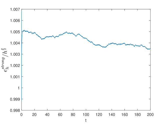
Figure 1: The approximation to $e^{strong}_{h}$ against $h^{\frac{p}{2}}$ over $[0,200]$

Example 25.

Consider a two dimensional SDE

$$d\left[\begin{array}[]{cc}x_{1}(t)\\ x_{2}(t)\end{array}\right] =\left[\begin{array}[]{cc}1+0.1x_{1}(t)-x_{2}(t)-21x_{1}^{3}(t)-21x_{1}^{5}(t)\\ 1+x_{1}(t)+0.1x_{2}(t)-21x_{2}^{3}(t)-21x_{2}^{5}(t)\end{array}\right]dt$$

$$\quad+\left[\begin{array}[]{cc}x_{1}(t)-0.2x_{2}(t)+x_{1}^{3}(t)-0.2x_{2}^{3}(t)\\ 0.2x_{1}(t)+x_{2}(t)+0.2x_{1}^{3}(t)+x_{2}^{3}(t)\end{array}\right]dW(t).$$

Let $l_{1}=20$, $l_{2}=5$ and $\alpha=\beta=0.025$, it is not hard to see that (8) -(12) are satisfied with $p=0.001$, $q=5$, $L_{1}=40$, $k_{1}=-21$, $c_{1}=20.5$, $c_{2}=10$, $k_{2}=-6$ and $c_{3}=5.5$. We use the BEM method to simulate 1000 sample paths with $x_{0}=[1,1]^{T}$ and $h=0.001$, and then the sample points generated by these paths at the same time point are used to construct the corresponding empirical density function. According to the (23), the underlying solution has a unique stationary distribution. However, its explicit form is hard to find. Therefore, to intuitively show that the underlying solution does have a unique stationary distribution, the empirical distribution at $t=5$ is regarded as the stationary distribution. Then we use the Kolmogorov-Smirnov test (K-S test) to measure the difference between the empirical distribution and the stationary distribution at each time point. As shown in Figure 2, the difference tends to 0, which indicates the numerical stationary distribution is quite a good approximation to the underlying one.

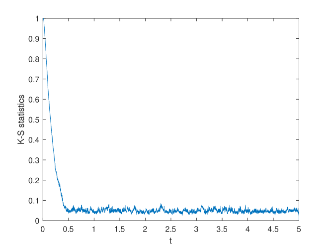
Figure 2: K-S statistics

5 Conclusion and future works

In this paper, a quite general result about the strong convergence in the infinite horizon of numerical methods for SDEs is proved. This result could cover many different numerical methods, as the proof does not need the detailed structure of the numerical methods.

In addition, as the driven noise are only required to be the independent and stationary, the results still hold if the Brownian motion is replaced by other proper processes.

Right now, we are working on a similar result for stochastic delay differential equation (SDDEs) and trying to build a connection between the numerical methods for SDEs and SDDEs.

References

- [1] A. Andersson and R. Kruse. Mean-square convergence of the BDF2-Maruyama and backward Euler schemes for SDE satisfying a global monotonicity condition. BIT Numer.Math., 57(1):21–53, 2017.
- [2] L. Angeli, D. Crisan, and M. Ottobre. Uniform in time convergence of numerical schemes for stochastic differential equations via strong exponential stability: Euler methods, split-step and tamed schemes. arXiv:2303.15463, 2023.
- [3] Z. Chen and S. Gan. Convergence and stability of the backward Euler method for jump-diffusion SDEs with super-linearly growing diffusion and jump coefficients. J. Comput. Appl. Math., 363:350–369, 2020.
- [4] D. Crisan, P. Dobson, and M. Ottobre. Uniform in time estimates for the weak error of the Euler method for SDEs and a pathwise approach to derivative estimates for diffusion semigroups. Trans. Amer. Math. Soc., 374(5):3289–3330, 2021.
- [5] K. Dareiotis, C. Kumar, and S. Sabanis. On tamed euler approximations of sdes driven by lévy noise with applications to delay equations. SIAM J. Numer. Anal., 54(3):1840–1872, 2016.
- [6] A. Gray, D. Greenhalgh, L. Hu, X. Mao, and J. Pan. A stochastic differential equation SIS epidemic model. SIAM J. Appl. Math., 71(3):876–902, 2011.
- [7] D.J. Higham and P.E. Kloeden. An introduction to the numerical simulation of stochastic differential equations. Society for Industrial and Applied Mathematics (SIAM), Philadelphia, PA, [2021] ©2021.
- [8] Y. Hu. Semi-implicit euler-maruyama scheme for stiff stochastic equations. In Stochastic analysis and related topics, V (Silivri, 1994), volume 38 of Progr. Probab., pages 183–202. Birkhäuser Boston, Boston, MA, 1996.
- [9] M. Hutzenthaler, A. Jentzen, and P.E. Kloeden. Strong convergence of an explicit numerical method for sdes with nonglobally lipschitz continuous coefficients. Ann. Appl. Probab., 22(4):1611–1641, 2012.
- [10] N. Ikeda and S. Watanabe. Stochastic differential equations and diffusion processes. North-Holland, Amsterdam, 1989.
- [11] P. E. Kloeden and E. Platen. Numerical Solution of Stochastic Differential Equations. Springer-Verlag, New York, 1992.
- [12] X. Li, X. Mao, and H. Yang. Strong convergence and asymptotic stability of explicit numerical schemes for nonlinear stochastic differential equations. Math. Comp., 90(332):2827–2872, 2021.
- [13] W. Liu and X. Mao. Numerical stationary distribution and its convergence for nonlinear stochastic differential equations. J. Comput. Appl. Math., 276:16–29, 2015.
- [14] W. Liu, X. Mao, and Y. Wu. The backward euler-maruyama method for invariant measures of stochastic differential equations with super-linear coefficients. Appl. Numer. Math., 184:137–150, 2023.
- [15] X. Mao. Stochastic Differential Equations and Applications. Horwood, Chichester, UK, 2 edition, 2007.
- [16] X. Mao. The truncated Euler-Maruyama method for stochastic differential equations. J. Comput. Appl. Math., 290:370–384, 2015.
- [17] M.V. Tretyakov and Z. Zhang. A fundamental mean-square convergence theorem for SDEs with locally Lipschitz coefficients and its applications. SIAM J. Numer. Anal., 51(6):3135–3162, 2013.
- [18] C. Yuan and X. Mao. Asymptotic stability in distribution of stochastic differential equations with markovian switching. Stochastic Process. Appl., 103(2):277–291, 2003.