Towards Anytime Optical Flow Estimation with Event Cameras

Abstract

Optical flow estimation is a fundamental task in the field of autonomous driving. Event cameras are capable of responding to log-brightness changes in microseconds. Its characteristic of producing responses only to the changing region is particularly suitable for optical flow estimation. In contrast to the super low-latency response speed of event cameras, existing datasets collected via event cameras, however, only provide limited frame rate optical flow ground truth, (e.g., at $10Hz$), greatly restricting the potential of event-driven optical flow. To address this challenge, we put forward a high-frame-rate, low-latency event representation Unified Voxel Grid, sequentially fed into the network bin by bin. We then propose EVA-Flow, an EVent-based Anytime Flow estimation network to produce high-frame-rate event optical flow with only low-frame-rate optical flow ground truth for supervision. The key component of our EVA-Flow is the stacked Spatiotemporal Motion Refinement (SMR) module, which predicts temporally dense optical flow and enhances the accuracy via spatial-temporal motion refinement. The time-dense feature warping utilized in the SMR module provides implicit supervision for the intermediate optical flow. Additionally, we introduce the Rectified Flow Warp Loss (RFWL) for the unsupervised evaluation of intermediate optical flow in the absence of ground truth. This is, to the best of our knowledge, the first work focusing on anytime optical flow estimation via event cameras. A comprehensive variety of experiments on MVSEC, DESC, and our EVA-FlowSet demonstrates that EVA-Flow achieves competitive performance, super-low-latency ($5ms$), fastest inference ($9.2ms$), time-dense motion estimation ($200Hz$), and strong generalization. Our code will be available at https://github.com/Yaozhuwa/EVA-Flow.

I Introduction

Optical flow estimation is of paramount importance in numerous computer vision applications, particularly in the domain of autonomous driving [1]. Optical flow estimation entails the computation of motion vectors for every pixel between successive frames, offering valuable insights into object movement within a given scene. In the realm of autonomous driving, precise optical flow estimation assumes utmost significance for critical tasks such as object tracking [2], collision estimation [3, 4], and scene parsing [5, 6, 7]. Moreover, optical flow estimation serves as a vital component within VO (Visual Odometry) and SLAM (Simultaneous Localization and Mapping) technology [8, 9, 10]. The accuracy of optical flow estimation directly affects the accuracy of subsequent autonomous perception tasks, making it a hot topic in the field of scene understanding [11, 12, 13, 14].

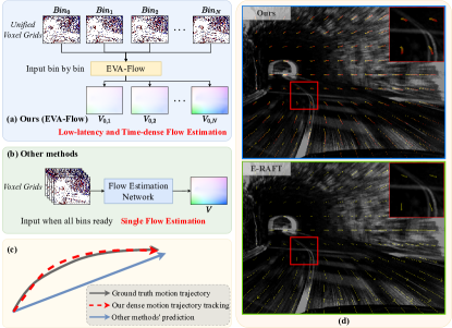
Figure 1: (a-b) EVA-Flow vs. previous event-based optical flow networks. Our Event-based Anytime optical Flow (EVA-Flow) framework achieves time-dense optical flow estimation with low latency, making it especially suitable for high-speed event cameras and safety-critical scenarios. (c) Comparison between our dense motion trajectory and other methods. (d) EVA-Flow’s dense motion trajectory vs. E-RAFT [15] on the DSEC dataset [16].

The event camera [17] is a new type of bio-inspired sensor that only responds to changes in the brightness of the environment. Compared with the traditional frame-based camera, which integrates the brightness at a certain time interval (exposure time) and outputs an image, the event camera has no exposure time and responds once the log value of the pixel intensity changes beyond a certain threshold, and the response is microsecond-level and asynchronous. As optical flow estimation aims to estimate the motion of a scene which aligns with the event camera’s ability to detect changes, it makes the event camera a suitable choice for optical flow estimation [18, 15]. Furthermore, event cameras offer distinct advantages for optical flow estimation, such as high temporal resolution and high dynamic range (${>}120dB$ compared to about $60dB$ of traditional frame-based cameras [17]). The high dynamic range capability of event cameras can solve the problem of under- or over-exposed images produced by traditional frame cameras in poor illumination conditions (such as at night) or high-dynamic scenes (such as cars entering and exiting tunnels) [19, 20], which can cause inaccurate optical flow estimation in subsequent processing. The high temporal resolution of event cameras eliminates the problem of motion blur even in high-speed motion scenes. Additionally, the high temporal resolution output of event cameras provides hardware support for super high-frame-rate optical flow estimation.

However, most current event-based optical flow estimation methods fail to fully exploit the high temporal resolution and low-latency characteristics of events, resulting in low frame rates for the estimated optical flow. They typically transform the event stream over a time interval into a tensor represented as voxels, which are then fed into a frame-based optical flow estimation network similar to image-based approaches [18, 21, 15]. Moreover, the output frame rate is limited by the underlying dataset. The two most commonly-used benchmarks for event-based optical flow estimation, MVSEC [22] and DSEC [16] have low frame rates for their ground-truth optical flow, with DSEC having a frame rate of $10Hz$ and MVSEC having a frame rate of $20Hz$. While significant progress has been witnessed in the field, the limited temporal resolution greatly restricts the potential of event-based optical flow estimation in real-world applications.

We present EVA-Flow, a deep architecture designed for Event-based Anytime optical Flow estimation. EVA-Flow delivers numerous benefits, such as low latency, high frame rate, and high accuracy. Fig. 1. (a-c) illustrates the differences between previous event-based optical flow estimation and our proposed approach toward anytime optical flow estimation. While other methods are limited by the dataset’s frame rate, this framework can achieve low latency and higher frame rate optical flow outputs. Fig. 1. (d) illustrates the discrepancy between the predictions of this model and E-RAFT using a sample from the test sequence of the DSEC dataset. The scene depicts a car making a turn inside a tunnel. Our EVA-Flow offers continuous trajectory tracking within a 100 ms time range of the input sample. The transition from yellow to red indicates varying point positions at different times in the trajectory of the car turning inside the tunnel. In contrast, E-RAFT [15] is restricted to generating a single optical flow.

To achieve high-frame-rate event output, we first propose the Unified Voxel Grid (UVG), which generates a bin of UVG representation as soon as the events in a small time interval are ready. Our UVG representation achieves a higher frame rate up to a factor of $N$ and a lower latency of $1/N$ compared to the voxel grid representation [21]. $N$ is a hyperparameter that can be adjusted to meet the specific requirements of the task. These bins are then sequentially fed into our EVA-Flow, which consists of a multi-scale encoder and our stacked Spatiotemporal Motion Recurrent (SMR) module. SMR is proposed to predict temporally dense optical flow and enhances the accuracy via spatial-temporal motion refinement. Notably, the architecture is specially designed for extreme low-latency optical flow estimation: as each event bin arrives, it is immediately processed through the SMR module, yielding the optical flow result for the current time instance. This architectural design eliminates the need to wait for all bins of the entire voxel grid to arrive in order to achieve high-frame-rate optical flow output.

Aside from the representation, for optical flow estimation, it is crucial to have a reliable method of measuring the consistency of the flow from one frame to the next. To achieve this, a loss function is usually designed to ensure that the optical flow converges. However, in the absence of ground truth for supervision, we do not directly supervise the intermediate optical flow, but instead, implicitly supervise it using the warping mechanism. Additionally, we introduce the Rectified Flow Warp Loss (RFWL) as a method to accurately assess the precision of event-based optical flow in an unsupervised manner. Moreover, we utilize RFWL to assess the accuracy of our time-dense optical flow estimation.

By comparing our EVA-Flow with other event-based optical flow estimation methods on widely recognized public benchmarks, including the DSEC [16] and MVSEC [22] datasets, we have determined that our approach attains performance comparable to the state-of-the-art E-RAFT [15] method, with the added benefits of lower latency ($5ms$ vs. $100ms$), higher frame rates ($200Hz$ vs. $10Hz$), and faster single-frame optical flow estimation speed ($9.2ms$ vs. $93ms$). Additionally, the evaluation of time-dense optical flow on DSEC, MVSEC, and EVA-FlowSet underscores the reliability of our framework’s time-dense optical flow, even under the constraint of being solely supervised with low-frame-rate optical flow ground truth during training. Furthermore, the Zero-Shot results obtained from both the MVSEC dataset and our EVA-FlowSet clearly illustrate that our method exhibits superior generalization performance in comparison to E-RAFT.

In summary, we deliver the following contributions:

• We present EVA-Flow, an Event-based Anytime optical Flow estimation framework that achieves high-frame-rate event-based optical flow with low-frame-rate optical flow ground truth as its sole source of supervision. EVA-Flow is characterized by its low latency, high frame rate, fast inference, and high accuracy.

• We propose the Unified Voxel Gird representation, which is of high frame rate and low latency.

• We propose RFWL to accurately evaluate the precision of event-based optical flow in an unsupervised manner.

• Extensive experiments on public benchmarks show EVA-Flow achieves competitive accuracy, super-low latency, fastest inference, time-dense motion estimation, and strong generalization.

II Related Work

II-A Optical Flow Estimation

Recently, the field of optical flow estimation has witnessed remarkable advancements owing to the progress of deep learning. FlowNet [23] firstly introduces an end-to-end network with a U-Net architecture to estimate optical flow directly from image frames and many subsequent works [24, 25, 26] follow this architecture. Later, [27, 28] utilize a warp mechanism to conduct a multi-scale refinement, achieving higher accuracy with less computational costs. RAFT [29] proposes a recurrent optical flow network that uses all-pair correlations and GRU iterations to produce high-precision flow results through iterative refinement, which achieves a significant improvement in accuracy. Most of the later optical flow studies are, in essence, improvements upon RAFT. CSFlow [30] introduces a decoupled strip correlation layer to enhance the capacity to encode global context. FlowFormer [31] explores the self-attention mechanism in recurrent flow networks to achieve further flow accuracy boosts, albeit with larger parameter usage. In summary, the use of warp mechanism, correlation volume, and RNN with iterative refinement has brought about significant advancements in the field of optical flow, allowing for improved accuracy and more efficient computation.

Unlike previous works, we explore anytime optical flow estimation with event cameras. We aim to overcome the limited time interval imposed by existing flow datasets and achieve ultra-high-frame-rate flow estimation with high accuracy.

II-B Event-based Optical Flow

Event optical flow estimation is mainly divided into model-based methods and learning-based methods. There are two main approaches to model-based event optical flow estimation. One approach is to fit the local spatiotemporal plane of the event point cloud and use the plane fitting parameters to compute the optical flow value [32, 33, 34]. Another approach builds on the contrast maximization framework [35], which calculates the optical flow by optimizing the contrast of the motion-compensated event frame [36]. However, model-based event optical flow algorithms [37, 32, 33, 34] generally require denoising algorithms like [38] for event preprocessing to improve the accuracy.

Thanks to the availability of large-scale event optical flow datasets [22, 16], learning-based event optical flow estimation algorithms [18, 21, 15] have achieved superior accuracy compared to model-based algorithms, which is also more robust to event noise. Next, we provide a brief review of works on learning-based event optical flow estimation.

EV-FlowNet [21] firstly utilizes bilinear interpolation on discrete events in both spatial and temporal dimensions. This transformation converts sparse and continuous events into a voxel-based tensor called Voxel Grid. Subsequently, the Voxel Grid is input to FlowNet [23] for estimating event optical flow. This paradigm has been adopted by numerous subsequent works [39, 15, 40, 41]. E-RAFT [15] achieves remarkable flow accuracy boosts by using event VoxelGrids with two-time intervals as the network’s input, recognized as the state of the art on the DSEC dataset [16]. Recently, TMA [42] and IDNet [43], have surpassed E-RAFT’s performance for their better utilization of the rich information in the temporal dimension of event data. The TMA network utilizes the temporal continuity of event input by calculating the correlation between the first bin and all other bins of the event Voxel Grid to acquire more precise motion information, achieving higher accuracy than E-RAFT with fewer iterations. IDNet sequentially feeds event Voxel Grids into RNN and estimates the flow for the entire time duration. Next, the network cascade and warp mechanisms conduct fine-grained processing on the flow, using the previously predicted flow in each cascade for direct deblurring of the event bins. While both TMA and IDNet make use of the continuous temporal information of event data, they can only achieve low-frame-rate optical flow outputs that match the frame rate of the ground truth, i.e., $10FPS$ on DSEC.

The event information provides brightness variation information of high temporal resolution, but only a few high-frame-rate event optical flow estimation methods are available. The limitation of the ground-truth frame rate of current datasets of event optical flow is one reason for this circumstance. Due to the lack of time-continuous ground truth, several studies [44, 45] have employed unsupervised contrast-maximization-based losses [36], resulting in lower accuracy for these methods. Ponghiran et al. [46] utilize recurrent neural networks to obtain temporally-dense optical flow results, which require sequential training and only evaluate the flow results at time locations with ground truth. The intermediate optical flow of this method has not undergone validation, and the final optical flow accuracy is relatively low. In contrast, our proposed approach, EVA-Flow, achieves a high level of accuracy, extremely low data latency, high frame rates, and excellent model generalization through comprehensive end-to-end training, requiring only low frame rate optical flow ground truth as supervision.

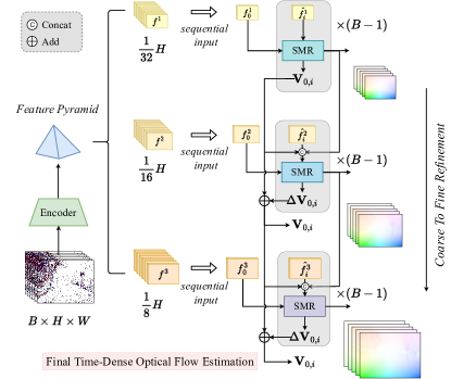
Figure 2: Overview of our proposed Event Anytime Flow Estimation (EVA-Flow) framework. The voxelized sequence input is processed sequentially by the encoder, and for each new event bin arrival, multi-scale feature maps are extracted. Based on these maps, the Spatiotemporal Motion Recurrent (SMR) module directly predicts optical flow for the time interval from $t_{0}$ to the current time step. $f^{i}$ denotes the features of the $i$-th level in a feature pyramid, while $f_{j}^{i}$ denotes the $j$-th event bin’s feature in $j^{i}$. $\mathbf{V}_{0,i}$ denotes flow prediction from time $t_{0}$ to $t_{i}$.

III Methodology

In this paper, we propose, for the first time, an Event Anytime Flow Estimation (EVA-Flow) framework, as shown in Fig. 2, which achieves high accuracy, high frame rate, and low latency with supervision solely dependent on low frame rate optical flow. EVA-Flow is designed to overcome the frame rate limitations of existing event-based optical flow datasets and produce temporally dense optical flow estimation with accuracy boosts compared to contemporary methods. We first put forward a Unified Voxel Grid Representation (UVG) in Sec. III-A, which generates event representations with low latency. These UVG bins are sequentially fed into EVA-Flow, where high-frame-rate optical flow estimations are generated with low latency using a Spatiotemporal Motion Recurrent (SMR) module, which is detailed in Sec. III-B. Then, the details of the loss function and the supervision regime are described in Sec. III-C. Finally, we propose a new criterion to evaluate the reliability of intermediate high-frame-rate optical flow in Sec. III-D.

III-A Event Representation: Unified Voxel Grid

To achieve anytime event-based optical flow estimation, we propose an Unified Voxel Grid (UVG) with high-frame-rate representations. The event representation is crucial for the event-based model [47, 48]. Voxel Grid [21] is a commonly used event representation that utilizes the temporal dimension of event data, and its effectiveness for optical flow estimation tasks has been verified in many studies [21, 15, 43]. The principle of the Voxel Grid is to discretize the spatially sparse and temporally-continuous information of events by averaging over time, and then utilize bilinear interpolation in both spatial and temporal dimensions to obtain a tensor representation of the event data in a voxel form. The tensor has a dimension of $B{\times}H{\times}W$, where $B$ represents the number of time steps, and its size determines the sampling accuracy of the event data in the temporal dimension. Each channel of the Voxel Grid can be viewed as an event representation at a specific time. Given a set of events $\left\{\left(x_{i},y_{i},t_{i},p_{i}\right)\right\}_{i\in[1,N]}$ and $B$ bins to discretize the time dimension, the definition of Voxel Grid is depicted as follows:

$$t_{i}^{*}=(B-1)\left(t_{i}-t_{1}\right)/\left(t_{N}-t_{1}\right),$$ (1)

$$k_{b}(a)=\max(0,1-|a|),$$

$$VG(x,y,t)=\sum_{i}p_{i}k_{b}\left(x-x_{i}\right)k_{b}\left(y-y_{i}\right)k_{b}\left(t-t_{i}^{*}\right),$$

where $k_{b}(a)$ denotes the bilinear sampling kernel.

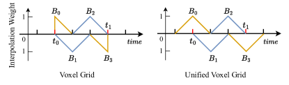
Figure 3: The proposed Unified Voxel Grid (UVG) compared with Voxel Grid [21]. The lines of different colors indicate the temporal scope of events encompassed in their respective bins, while the vertical axis of each line represents the interpolated weight of the events at the point in time. Various line colors are employed to differentiate among adjacent event bins.

To achieve continuous predictions of high-frame-rate optical flow, it is necessary to obtain high-frame-rate event representations. Every input requires a uniform format for event representation. However, the Voxel Grid [21] represents the first and last channels differently as compared to the others, as shown in Fig. 3. The event interpolation time range utilized for the first and last channels in the Voxel Grid is half of that used for the other channels, leading to inconsistency, which is adverse to continuous predictions. As a solution, we propose Unified Voxel Grid. In contrast to Voxel Grid, we fix the time interval $\tau$ for each bin. And each bin is created through the interpolation of events from the adjacent $\tau$ time-step ($t_{b}-\tau<e_{i}[t]<t_{b}+\tau$). The definition of UVG is depicted as follows:

$$Bin_{b}(x,y)=\sum_{i}p_{i}k_{b}\left(x-x_{i}\right)k_{b}\left(y-y_{i}\right)k_{b}\left(\frac{t-t_{b}}{\tau}\right)$$ (2)

$$UVG=concat([Bin_{0},Bin_{1},...,Bin_{B-1}]).$$

This design makes it possible to obtain the current representation of time for each $\tau$ ($7.14ms$ for $15$ channels with Unified Voxel Grid on DESC), while the Voxel Grid must wait for the entire period of $(B-1)\times\tau$ ($100ms$ on DSEC) to generate a complete event representation. This low-latency input can be coupled with our low-latency time-dense optical flow estimation architecture for tracking the optical flow at each $\tau$ timestep as it arrives which is essential for high-frame-rate optical flow estimation.

III-B Event Anytime Flow Estimation Framework

In this subsection, we propose the Event Anytime Flow (EVA-Flow) framework, which predicts time-dense optical flow from serial event bins with low latency. The architecture of EVA-Flow is illustrated in Fig. 2. The raw events are converted to UVG and then sequentially fed into the encoder, bin by bin, to generate a 4-level feature pyramid ($f_{i}^{1}{\to}f_{4}^{N}$). The feature pyramid is fed into our stacked Spatiotemporal Motion Recurrent (SMR) modules to update the optical flow in both temporal and spatial dimensions while outputting the refined optical flow results from $t_{0}$ to the current bin.

Serialized, low-latency input and output. The UVG inputs are sequentially fed into the network, which contributes to the low latency at the data entry level. During the inference phase, after entering an event bin (excluding the first bin used for initialization), the current optical flow can be directly predicted using the encoder and the stacked SMR module. During the training phase, in order to facilitate end-to-end training, we follow the frame rate of the dataset and input a full period of UVG at once as a training sample. Following the UVG input of $N,B,H,W$, the UVGs of different bins (i.e. with different channels) are converted to the batch dimension and concatenated (resulting in a dimension of $N{\times}B,H,W$) before being passed through the encoder. Once the feature maps are obtained, the corresponding feature maps of different bins are sequentially input into the stacked SMR module, which outputs time-dense optical flow ($\mathbf{V}_{0,1}\to\mathbf{V}_{0,B-1}$).

Spatiotemporal Motion Recurrent (SMR) module.

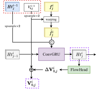
Figure 4: The proposed Spatiotemporal Motion Recurrent (SMR) module. The red dashed box encloses the output of the SMR module in the preceding feature pyramid layer, and the purple box surrounds the output of the current feature pyramid layer’s SMR module, which will transfer to the SMR module of the next layer in the feature pyramid.

In order to predict time-dense optical flow and achieve high accuracy through iterative refinement, we propose the stacked SMR modules, whose structure is illustrated in Fig. 4. In the vertical direction, as illustrated in Fig. 2 and Fig. 4, SMR performs an iterative refinement of optical flow at the current moment in the spatial dimension. The input of this module includes the hidden state of the lower-resolution SMR module from the previous level, the optical flow output, and the feature inputs of the current resolution level. First, we warp the input feature $f_{j}^{i}$ using the rough optical flow estimated from the previous level to obtain the post-warp features $\hat{f_{j}^{i}}$. Next, the optical flow $\mathbf{V}_{0,j}^{i-1}$ from the previous level, the warped features, and the upsampled hidden state $Ht_{j}^{i-1}$ from the previous level are concatenated, and used as input for the Convolutional Gated Recurrent Unit (ConvGRU) [49]. Subsequently, the hidden state output of the current ConvGRU is used by the Flow Head to predict the residual optical flow. We employ two convolutional layers for the Flow Head, which is the same as RAFT [29]. The refined optical flow $\mathbf{V}_{0,j}^{i}$ is achieved by adding the predicted residual optical flow $\Delta\mathbf{V}_{0,j}^{i}$ to the previously predicted optical flow $\mathbf{V}_{0,j}^{i-1}$. The current level’s predicted optical flow and hidden state are also inputted to the next level in the same way, for further refinement. This continues until the final level predicts the ultimate refined optical flow.

In the horizontal direction in Fig. 2, SMR continuously estimates optical flow at each time step. In general, SMR serves as a motion-updating module in both spatial and temporal dimensions. Within the same layer in the horizontal direction, SMR modules leverage shared weights, while in the vertical direction, different SMR weights are used due to varying input resolutions and channel numbers. In general, the number of SMRs is equal to the number of levels for spatial refinement of the optical flow estimation.

Time-dense feature warping. Unlike other methods [43, 42] that rely on the assumption of uniform motion between two ground-truth flows, our approach can handle variations in motion speeds throughout the entire UVG period. In each warping step, we use the dense temporal optical flow estimation of the previous level to warp the features of each time step. This structure guarantees consistent prediction patterns of optical flow for each resolution level and time step (SMR modules at the same level are using shared weights), implicitly providing SMR modules with the ability to predict optical flow at the current time step. By implementing this approach, we only need to supervise the final output $\mathbf{V}_{0,B-1}$ for implicit monitoring of optical flow at intermediate time steps.

III-C Supervision

Following E-RAFT [15], we also used L1 loss as the loss function. Specifically, we calculate the L1 distance between the ground-truth optical flow and the last optical flow prediction $\mathbf{V}_{0,B-1}$ of our model as the final loss function. The loss function is defined as follows:

$$Loss=||\mathbf{F}_{gt}-\mathbf{F}_{pre}||_{1}.$$ (3)

Due to network structure design (see explanation in Sec. III-B in Time-dense feature warping), we don’t need to supervise the optical flow prediction at intermediate time steps. In this way, we overcome the frame rate limitation of the dataset and achieve low-latency, high-frame-rate, and high-precision event optical flow estimation.

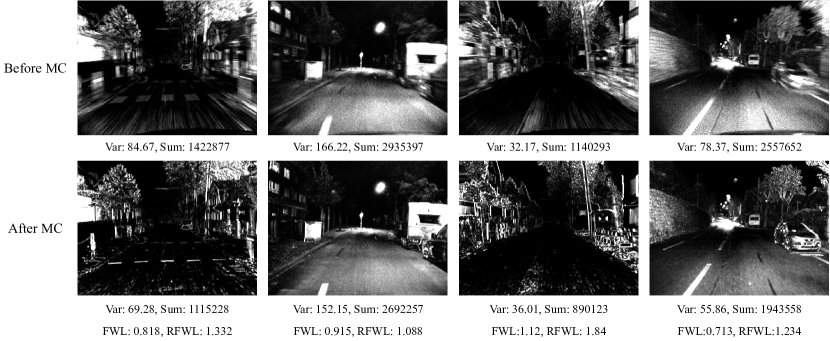
Figure 5: RFWL vs. FWL. The first row shows the event count images generated by the original event stream of the DSEC test sequences [16], while the second row shows the event count images generated by the motion-compensated event stream using our flow estimation, which we name MC frames. Each image is annotated with the variance and sum of pixel values (corresponding to the number of events detected in the respective image regions). The last row presents the FWL and RFWL of the motion-compensated frames (MC frames) for distinct columns.

III-D Rectified Flow Warp Loss

Motion compensation [35] of events involves aligning all events to a reference time using estimated event optical flow. Specifically, for every event, using the flow value of the event position and the time difference between the event occurrence time and the reference time, we can calculate the position of the event point at the reference time. This process is referred to as motion compensation. The motion-compensated event count image is called a Motion-Compensated (MC) event frame.

Given events $E=(\left\{\left(x_{i},y_{i},t_{i},p_{i}\right)\right\}_{i\in[1,N]})$, per-pixel flow estimation $\mathbf{V}$ and a reference time $t^{\prime}$, the MC frame is defined as follow:

$$I(E,\phi)=\left(\begin{array}[]{l}x_{i}^{\prime}\\ y_{i}^{\prime}\end{array}\right)=\left(\begin{array}[]{l}x_{i}\\ y_{i}\end{array}\right)+\left(t^{\prime}-t_{i}\right)\mathbf{V}(x_{i},y_{i}).$$ (4)

Accurate flow estimation ensures that events generated by the same edge are aligned to the same pixel location, resulting in higher contrast in the MC frame than in the original event frame. Stoffregen et al. [50] utilized this principle to propose a Flow Warp Loss (FWL), which can assess the accuracy of event optical flow estimation in an unsupervised way.

$$\mathrm{FWL}:=\frac{\sigma^{2}(I(E,\mathbf{V}))}{\sigma^{2}(I(E,0))}$$ (5)

In theory, a more accurate estimation of optical flow results in a clearer, higher contrast, and larger variance for the image after motion compensation. This is because events occurring at the same location in the scene are aligned to the same point. Therefore, a more accurate prediction of optical flow leads to a larger FWL. In general, the image tends to become sharper after motion compensation, indicating an FWL value greater than $1$. However, in practice, we observe that FWL can be smaller than $1$, yet the MC frame is clearly sharper than the original one, as shown in Fig. 5. We have identified the same phenomena (FWL <1) in another work [36]. After analysis, we discover that motion compensation has warped some events out of the image, resulting in fewer events in the MC frame compared to the original frame. Thus, we propose a Rectified Flow warp Loss (RFWL), which normalizes image brightness based on the total event count (i.e., the sum of pixel values) in the event frames before and after motion compensation. The formulation is given as follows:

$$\mathrm{RFWL}:=\sigma^{2}(\frac{I(E,\mathbf{V})}{\sum I(E,\mathbf{V})})/\sigma^{2}(\frac{I(E,0)}{\sum I(E,0)}).$$ (6)

As shown in Fig. 5, FWL is inadequate at precisely assessing the accuracy of optical flow estimation. MC frames, as shown in columns 1, 2, and 4 exhibit sharper resolution compared to the original event frames, whereas the FWL values remain less than $1$. Interestingly, the MC frame in column 3, which has a significantly sharper resolution than the original event frame, yields an FWL value of only $1.12$. The FWL values of these examples are inconsistent with the actual observational results. Conversely, our proposed RFWL can precisely indicate the relative sharpness of MC frames in relation to the original event frames.

IV Experiments

Our model underwent evaluation on the DSEC [16], MVSEC [18], and self-collected EVA-FlowSet. Sec IV-A offers an introduction to the aforementioned datasets. Sec. IV-B presents the implementation details of our approach. Sec. IV-C demonstrates the evaluation of our model using the regular flow evaluation prototype. Sec. IV-D reveals the evaluation results of our model for time-dense optical flow. Sec. IV-E encompasses ablation studies.

IV-A Datasets

DSEC. The DSEC dataset, introduced by Gehrig et al. [16], consists of $24$ sequences captured in real-world outdoor driving scenes. The dataset includes a total of $7,800$ training samples and $2,100$ testing samples, captured at a resolution of $640{\times}480$. It covers both daytime and nighttime scenarios, encompassing small and large optical flows. Moreover, the DSEC dataset offers high-precision sparse ground truth values for optical flow. As the dataset does not include an official validation set, we divided the training dataset randomly using a fixed seed. To create the training and validation sets, we allocated them in a $4{:}1$ ratio. Consequently, only $80\%$ of the training data was utilized for training our model.

MVSEC. MVSEC [18] is a classic real event optical flow dataset that comprises sequences from various indoor and outdoor scenes with a resolution of $346{\times}260$. The event density of the dataset is relatively sparse, and the optical flow ground truth distribution mostly highlights small flows. As a result, two different time intervals, i.e., $dt{=}1$ and $dt{=}4$, are used for accuracy evaluation. $dt{=}1$ means that adjacent grayscale frames are used as a sample, whereas $dt{=}4$ represents a four-fold increase in the grayscale frame interval. We follow the E-RAFT convention [15], conduct training solely on the outdoor day 2 sequence, and evaluate on $800$ samples data from outdoor day 1.

EVA-FlowSet. We collect and present EVA-FlowSet, a real-world dataset to assess the generalization and time-dense optical flow of our model. For data collection, we utilized a Davis-346 camera, which is the same type used in the MVSEC dataset. The dataset consists of four sequences in total, with two sequences depicting fast-moving scenes and the other two showcasing regular motion scenes. During the data-collection process, the camera remains stationary, capturing the movement of a checkerboard calibration board as it travels along a curved trajectory at different predetermined speeds.

IV-B Implementation Details

For the DSEC dataset [16], we use the Adam optimizer with a batch size of $6$ and a learning rate of $5{\times}1e^{-4}$ to train for $100k$ iterations on the training set we divided, which accounts for $80\%$ of the total dataset. Then, we reduce the learning rate by a factor of $10$ and continue training for another $10k$ iterations. We applied the same training settings to networks employing different numbers of bins. During the model training on the DSEC dataset, two online data augmentation methods, namely random cropping and horizontal flipping, were employed. Random cropping was performed with a size of $288{\times}384$, while horizontal flipping was applied with a probability of $50\%$.

For the MVSEC dataset [18], we employ the Adam optimizer with a batch size of $3$ and a learning rate of $1{\times}1e^{-3}$ to train for $120k$ iterations. We utilize random cropping with a size of $256{\times}256$ and horizontal flipping with a probability of $50\%$ during training. For MVSEC scenes with $dt{=}1$, we use the setting with $bins{=}3$; for MVSEC with $dt{=}4$, we use the setting with $bins{=}9$.

TABLE 1: Evaluation results on the DSEC hidden test set [16].

Methods	EPE$\downarrow$	AE$\downarrow$	1PE$\downarrow$	3PE$\downarrow$	Runtime
					(ms per prediction)
Shiba et al. [36]	3.47	13.98	76.57	30.86	-
EV-FlowNet [18]	2.32	7.90	55.4	18.6	18
E-RAFT [15]	0.82	-	13.5	3.0	93
IDNet 1 iter [43]	1.30	4.82	33.7	6.7	-
TIDNet† [43]	0.93	3.98	19.3	3.4	-
EVA-Flow (Ours)	0.88	3.31	15.9	3.2	9.2
E-RAFT† [15]	0.79	2.85	12.7	2.7	93

† denotes that the method uses the warm-start strategy.

IV-C Regular Flow Evaluation Prototype

Evaluation on DSEC. Tab. 1 displays the evaluation results on the DSEC flow benchmark [16]. It is worth noting that this approach is the only optical flow estimation method that has ultra-low data latency ($5ms$) and a high output frame rate ($200Hz$), while also achieving competitive accuracy compared to state-of-the-art methods. This approach can estimate the current optical flow as soon as the event data arrives every $5ms$, without needing to wait for the entire sample period ($100ms$) to be completed, resulting in extremely low data latency and a super high frame rate($200Hz$). In contrast, other approaches, constrained by the frame rate of the ground truth dataset, can only provide optical flow outputs at 10 Hz. Furthermore, the computational cost of a single optical flow estimation in this approach is remarkably low. Our runtime for a single optical flow estimation is the lowest among other methods, with only $10\%$ of E-RAFT’s runtime. The runtime was obtained by testing on the 2080Ti.

The qualitative results of our method on the DSEC flow dataset are shown in Fig. 6. To make a more intuitive comparison of the accuracy of optical flow estimation, we also visualized the motion-compensated (MC) event frames. The sharper the MC frames, the more precise the optical flow estimates. It can be seen from the Regions of Interest (ROIs) in Fig. 6 that, compared with E-RAFT, our model can better distinguish the outline of small objects (such as poles) and obtain more accurate optical flow estimates. Our analysis indicates that the implicit use of warp-aligned edges of events in our approach to obtain motion features is the distinguishing factor compared to E-RAFT, which instead uses correlation volume. For small objects with simple and clear contours, it is relatively easy to warp and align event features. However, due to the limited textures, the correlation-based method, which relies on measuring feature similarity to obtain motion features, fails to obtain high-quality motion features when there are no sufficient texture features, resulting in the inferior performance of E-RAFT in these areas.

TABLE 2: Evaluation results on MVSEC [18].

$dt{=}1$		EPE $\downarrow$	Outlier%$\downarrow$
SSL	EV-FlowNet [18]	0.49	0.20
	Spike-FlowNet [51]	0.49	-
	STE-FlowNet [52]	0.42	0.00
USL	Hagenaars et al. [53]	0.47	0.25
	Zhu et al. [21]	0.32	0.00
	Shiba et al. [36]	0.30	0.10
SL	E-RAFT [15]	0.24	0.00
	EVA-Flow (Ours)	0.25	0.00
	E-RAFT [15] (Zero-Shot)	0.53	1.42
	EVA-Flow (Zero-Shot)	0.39	0.07
$dt{=}4$
SSL	EV-FlowNet [18]	1.23	7.30
	Spike-FlowNet [51]	1.09	-
	STE-FlowNet [52]	0.99	3.90
USL	Hagenaars et al. [53]	1.69	12.5
	Zhu et al. [21]	1.30	9.70
	Shiba et al. [36]	1.25	9.21
SL	E-RAFT [15]	0.72	1.12
	EVA-Flow (Ours)	0.82	2.41
	E-RAFT [15] (Zero-Shot)	1.93	17.7
	EVA-Flow (Zero-Shot)	0.96	4.92

TABLE 3: Comparison of anytime flow estimation on DSEC [16].

Sequence	Method	RFWL														Avg.	Runtime (ms/frame)
		$\mathbf{V}_{0\xrightarrow{}1}$	$\mathbf{V}_{0\xrightarrow{}2}$	$\mathbf{V}_{0\xrightarrow{}3}$	$\mathbf{V}_{0\xrightarrow{}4}$	$\mathbf{V}_{0\xrightarrow{}5}$	$\mathbf{V}_{0\xrightarrow{}6}$	$\mathbf{V}_{0\xrightarrow{}7}$	$\mathbf{V}_{0\xrightarrow{}8}$	$\mathbf{V}_{0\xrightarrow{}9}$	$\mathbf{V}_{0\xrightarrow{}10}$	$\mathbf{V}_{0\xrightarrow{}11}$	$\mathbf{V}_{0\xrightarrow{}12}$	$\mathbf{V}_{0\xrightarrow{}13}$	$\mathbf{V}_{0\xrightarrow{}14}$
thun_01_a	E-RAFT*	1.039	1.104	1.163	1.211	1.250	1.282	1.309	1.333	1.355	1.374	1.392	1.407	1.422	1.434	1.291	93
	EVA-Flow (Ours)	1.030	1.101	1.166	1.217	1.256	1.289	1.316	1.339	1.359	1.379	1.394	1.408	1.421	1.434	1.294	9.2
thun_01_b	E-RAFT*	1.058	1.134	1.193	1.236	1.277	1.313	1.349	1.382	1.416	1.447	1.476	1.500	1.522	1.539	1.346	93
	EVA-Flow (Ours)	1.046	1.135	1.208	1.262	1.305	1.340	1.370	1.393	1.419	1.444	1.467	1.490	1.512	1.532	1.352	9.2
interlaken_01_a	E-RAFT*	1.098	1.218	1.316	1.406	1.483	1.552	1.624	1.694	1.758	1.816	1.868	1.911	1.947	1.970	1.619	93
	EVA-Flow (Ours)	1.084	1.218	1.332	1.437	1.519	1.585	1.645	1.705	1.758	1.810	1.857	1.898	1.934	1.961	1.625	9.2
interlaken_00_b	E-RAFT*	1.105	1.233	1.338	1.426	1.500	1.565	1.621	1.670	1.714	1.753	1.788	1.819	1.843	1.860	1.588	93
	EVA-Flow (Ours)	1.088	1.229	1.340	1.437	1.515	1.576	1.626	1.670	1.709	1.742	1.770	1.796	1.816	1.837	1.582	9.2
zurich_city_12_a	E-RAFT*	1.005	1.020	1.034	1.050	1.065	1.079	1.090	1.103	1.116	1.127	1.139	1.149	1.161	1.169	1.093	93
	EVA-Flow (Ours)	1.004	1.021	1.032	1.046	1.060	1.075	1.085	1.099	1.111	1.122	1.134	1.145	1.157	1.166	1.090	9.2
zurich_city_14_c	E-RAFT*	1.057	1.155	1.250	1.329	1.391	1.453	1.510	1.555	1.598	1.636	1.666	1.695	1.724	1.752	1.484	93
	EVA-Flow (Ours)	1.044	1.152	1.249	1.333	1.394	1.460	1.517	1.561	1.605	1.645	1.675	1.704	1.732	1.761	1.488	9.2
zurich_city_15_a	E-RAFT*	1.071	1.174	1.256	1.324	1.384	1.436	1.480	1.522	1.566	1.606	1.642	1.676	1.703	1.721	1.469	93
	EVA-Flow (Ours)	1.062	1.177	1.270	1.345	1.409	1.461	1.502	1.542	1.580	1.614	1.646	1.677	1.701	1.720	1.479	9.2

E-RAFT* indicates that the intermediate flow is obtained by interpolating the E-RAFT predictions over the complete time range.

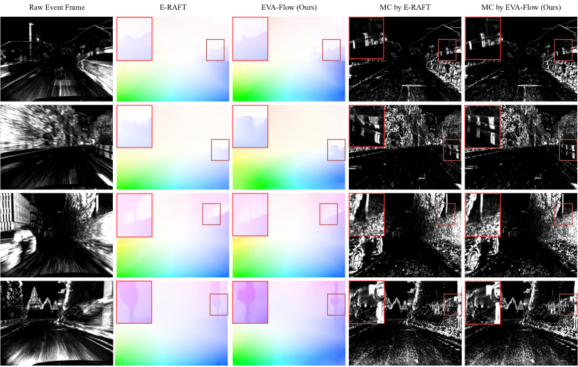
Figure 6: Qualitative examples of optical flow predictions on the DSEC test sequences [16]. The four samples are obtained from different scenes belonging to distinct sequences. The areas of interest are demarcated by red boxes in the images. These regions are enlarged by a factor of two and presented in the upper left corner of the corresponding images. The abbreviation MC represents motion-compensated.

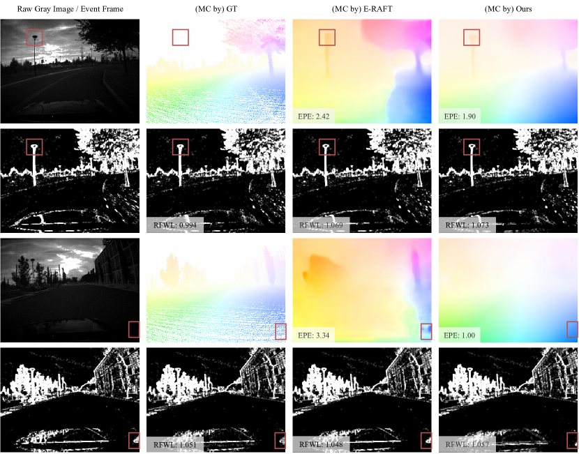
Figure 7: Qualitative examples of optical flow predictions on the outdoor day 1 sequence of the MVSEC dataset [18] ($dt{=}4$). The model used here is only trained on the DSEC dataset [16]. The respective EPE and RFWL metrics can be found in the bottom left corner of the images. The areas of interest are denoted as red boxes in the images.

Evaluation on the MVSEC dataset. The evaluation results of the MVSEC benchmark [18] are presented in Tab. 2. SSL, USL, and SL stand for self-supervised-, unsupervised-, and supervised learning, respectively. While our model’s accuracy is slightly lower than that of E-RAFT based on the data in the table, it is worth highlighting that our zero-shot results display a significantly better accuracy when directly testing the performance of the DSEC-trained model on the MVSEC dataset. Especially noteworthy is our model’s performance at $dt{=}4$, where our model’s EPE is halved compared to that of E-RAFT ($0.96$ vs. $1.93$). These results demonstrate the superior generalizability of the proposed EVA-Flow.

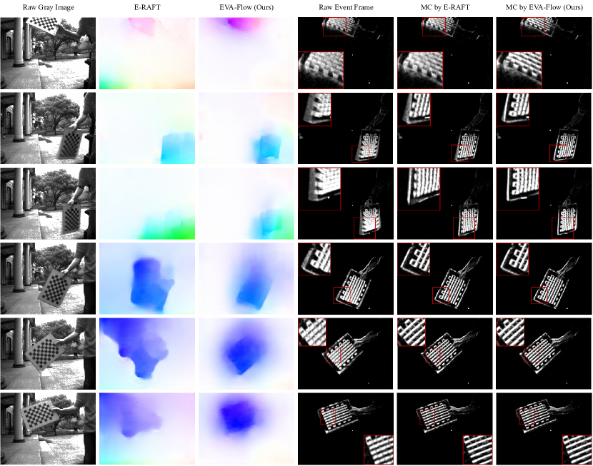
Figure 8: Qualitative examples of optical flow predictions on our EVA-FlowSet. The model used here is only trained on the DSEC dataset [16]. The initial three rows of samples are obtained from high-speed sequences, while the remaining three rows are taken from normal-speed ones. Best view via zoom in.

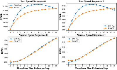
Figure 9: Evaluation results of time-dense optical flow using the RFWL in EVA-FlowSet. Models utilized here are exclusively trained on the DSEC dataset [16]. Our proposed model significantly outperforms E-RAFT in fast-motion scenarios.

The qualitative results of testing MVSEC under the zero-shot setting, i.e., the model is only trained on DSEC, can be found in Fig. 7. Owing to the small optical flow of MVSEC, the motion compensation effect is indistinct under the $dt{=}1$ setting. Hence, we apply a longer time range of grayscale frames, i.e., $dt{=}4$. There is a marked discrepancy in motion speed between the MVSEC and DSEC datasets, as depicted in Fig. 7 and Fig. 6. More specifically, the event images in the MVSEC dataset display minimal motion blur caused by slow movement, whereas the DSEC dataset showcases significant motion blur attributed to rapid motion. Nonetheless, our model is capable of achieving near-ground-truth optical flow results on the MVSEC dataset, while E-RAFT shows inadequate generalization performances, particularly in non-event ground areas. Additionally, our model demonstrates superior capabilities for small targets such as poles and road markings, accurately depicting their contours with improved motion compensation results.

Evaluation on EVA-FlowSet. Qualitative results of the curve motion scene dataset EVA-FlowSet can be found in Fig. 8. By visualizing the optical flow images, it can be observed that, for both fast-moving scenes and normal scenes, our model can estimate the contour of moving objects more accurately than E-RAFT [15]. The magnified ROI area shows that our model obtains sharper motion compensation results in the first three rows of fast-moving scenes, while E-RAFT’s motion compensation performance is comparable to our model in the last three rows of moderate-moving-speed scenes. E-RAFT calculates the correlation between the event voxel grid before and after the start time to estimate the optical flow, which implicitly assumes that the optical flow is constant throughout the entire time. In contrast, our method uses the SMR module iteratively in each time step to obtain continuous optical flow estimation, which is suitable for curve motion scenes. For moderate-moving-speed scenes, even if the motion trajectory is curved, the motion could be approximated as linear due to the slow motion speed. In moderate-moving-speed cases, E-RAFT’s motion compensation result is comparable to our model. However, in fast-moving scenes, the linear motion assumption of E-RAFT is no longer valid due to the curved nature of the motion trajectory. This scenario is particularly critical for safety concerns. In contrast, our model utilizes a dense optical flow estimation framework that does not depend on the linear motion assumption. Consequently, our model significantly outperforms E-RAFT in fast-moving scenes.

IV-D Time-Dense Optical Flow Evaluation

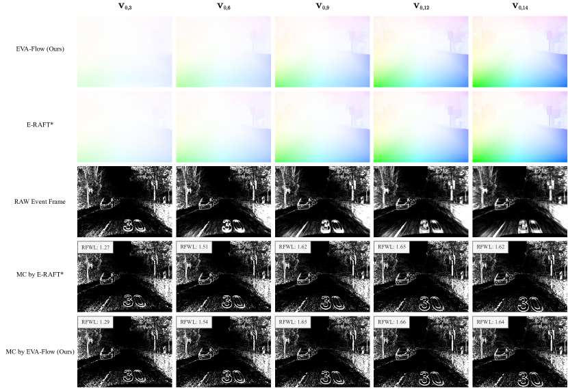
Figure 10: Illustration of our time-dense optical flow evaluation. Each row in the table shows the results of different time steps within a DSEC sample window of $100ms$ (total $14$ steps under $bins{=}15$). E-RAFT* indicates that the results at the intermediate time steps are obtained by interpolating the E-RAFT predictions over the complete time range.

As the DSEC flow dataset does not provide high frame-rate optical flow ground truth, we are not able to evaluate the precision of our model for temporally dense optical flow directly using the EPE metric. We propose a new unsupervised metric called RFWL to address this issue and assess the precision of event-based optical flow. Please refer to Sec. III-D for more details. Under the setting of $bins{=}15$, our model can obtain $14$ consecutive optical flow estimates for every sample from events occurring within $100ms$ on the DSEC test dataset. The output $V_{0,i}$ represents the optical flow estimation ranging from $0ms$ to $100{\times}\frac{i}{14}ms$. In contrast, E-RAFT is limited to obtaining single optical flow estimates within the time range of $0ms$ to $100ms$. Due to the absence of time-dense ground truth in the DSEC dataset, we directly compare our model with E-RAFT. We use time-dense optical flow results from our model and E-RAFT’s interpolated optical flow to generate motion-compensated frames for events during the relevant time periods. The demonstration of this process is shown in Fig. 10. We evaluate all test sequences for the DESC-Flow dataset and provide the detailed data in Tab. 3. Among the evaluated seven sequences, our model outperforms E-RAFT in terms of average RFWL in five sequences. Since movement in the DSEC dataset is predominantly linear, direct interpolation already yields relatively accurate intermediate optical flow. As a result, our method surpasses E-RAFT by small yet consistent margins on this dataset. Additionally, our runtime for a single optical flow estimation is only $10\%$ ($9.2ms$ vs. $93ms$) of E-RAFT’s runtime.

TABLE 4: Ablations of event representation ($bins{=}15$).

Event Representation	AE $\downarrow$	EPE $\downarrow$	1PE $\downarrow$	3PE $\downarrow$
Voxel Grid [21]	3.48	0.96	17.7	3.65
Unified Voxel Grid	3.39	0.89	16.1	3.30

We perform the same comparison on the EVA-FlowSet, which consists of sequences with curved movements. The results, depicted in Fig. 9, clearly indicate a substantial performance improvement achieved by our approach in comparison to E-RAFT. Since our EVA-FlowSet does not provide ground truth optical flow, both E-RAFT and our model rely on checkpoints trained on the DSEC dataset. Fig. 9 presents a visual representation of the evaluation results comparing our method with E-RAFT in diverse real-world scenarios with varying motion speeds. Specifically, in two fast-moving sequences, our model demonstrates a notably superior intermediate RFWL compared to E-RAFT. This occurs due to the nonlinearity of the optical flow caused by the curved trajectory. Consequently, the interpolated intermediate flow obtained from E-RAFT’s prediction proves notably less accurate compared to the time-dense flow predicted by our model. In the other two scenarios with normal-speed sequences, this model and E-RAFT exhibit comparable RFWL performance. When the movement speed is not fast enough during motion along a curved trajectory, the motion can be approximated as linear for a brief duration. We observe that the overall accuracy of EVA-Flow is notably higher during fast motion, and it exhibits a little decrease in accuracy towards the end of the event bin cycle. While it’s true that the design of a continuous warp mechanism introduces the potential for error accumulation, we argue that given the smaller number of parameters and low computational costs associated with EVA-Flow, this drawback can be easily mitigated by periodically resetting the forward propagation process.

As depicted in Fig. 8, the qualitative results affirm that our model outperforms E-RAFT in distinguishing motion boundaries, even in scenarios with normal speed. Notably, E-RAFT tends to erroneously extend the optical flow from motion regions to non-motion regions. However, since non-motion regions have few events, any inaccuracies in optical flow estimation will have no impact on the results of motion compensation. Consequently, in this specific situation, the RFWL of E-RAFT is comparable to that of this model. Overall, our proposed EVA-Flow is evidenced to be superior in time-dense flow estimation both numerically and qualitatively.

To assess the effectiveness of our time-dense optical flow estimation framework from an alternative perspective, we employ a different approach for the MVSEC dataset. In Tab. 2, we present the zero-shot results of E-RAFT and our model (trained only on DSEC and directly tested on MVSEC, $bins{=}15$). When evaluating the optical flow estimation on the MVSEC dataset using our model, we utilize the same model checkpoint but employ varying bin numbers based on different $dt$ values. As a result of the divergence in motion speeds between the slow-motion MVSEC dataset and the fast-motion DSEC dataset, we assign $bins{=}4$ for $dt{=}1$ and $bins{=}13$ for $dt{=}4$. This setting is based on the number of bins in our model minus $1$, which equals the number of the time-dense optical flow output. Therefore, under this setting, the frame rate of the optical flow output with $dt{=}4$ is exactly equal to the frame rate of the optical flow output with $dt{=}1$. And when $dt{=}4$ is utilized, it corresponds to an ongoing iteration of the SMR module using $dt{=}1$ time step until the optical flow for the entire duration can be forecasted.

By analyzing the data presented in Tab. 2, it is apparent that our model achieves a lower endpoint error (EPE) of $0.96$ at $dt{=}4$, which is less than four times the EPE at $dt{=}1$ ($0.39$). Interestingly, the results indicate that as we progressively iterate and generate optical flow for longer time intervals, the average per-unit-time optical flow error does not increase, but rather decreases. These findings provide clear evidence for the efficacy of our framework in estimating time-dense optical flow. Moreover, this highlights a key benefit of the adaptable implementation of this framework. It allows for flexible adjustment of the number of prediction bins, enabling a reduction in the event rate discrepancy per bin between training and prediction data, thus achieving higher accuracy in the deployment stage.

IV-E Ablation Study

TABLE 5: Ablation on the bins setting.

Bins	Latency/FPS	EPE $\downarrow$	AE $\downarrow$	1PE $\downarrow$	3PE $\downarrow$
6	$20ms$ / $50Hz$	0.955	3.29	16.7	3.9
11	$10ms$ / $100Hz$	0.926	3.34	16.1	3.5
15	$7.1ms$ / $140Hz$	0.895	3.39	16.1	3.3
21	$5ms$ / $200Hz$	0.877	3.31	15.9	3.2
31	$3.3ms$ / $300Hz$	0.901	3.37	17.0	3.2

Unified Voxel Grid. Tab. 4 compares the results of our framework on the DSEC test set using Voxel Grid [21] and our proposed Unified Voxel Grid representation. The EPE of our proposed Unified Voxel Grid is $7.3\%$ lower than that of Voxel Grid. This difference stems from the fact that each event bin in the Unified Voxel Grid adheres to a consistent event representation, while the representation patterns of the first and last bins in the Voxel Grid do not match those of the middle bins (refer to Fig. 3).

Investigate Bins Setting. The design of the proposed framework enables an increase of the optical flow output’s frame rate by increasing the number of bins in a $100ms$ sample from the DSEC dataset. It is essential to ensure that each bin has a sufficient number of events to encompass the motions taking place within the scene. In this study, the number of event bins varies from $6$ to $31$. Tab. 5 illustrates a consistent decrease in the final endpoint error (EPE) of event optical flow as the number of bins increases from $6$ to $21$. This trend is attributed to the reduction in complexity during optical flow estimation in each iteration when a higher number of bins is used. This reduction is due to a smaller amount of optical flow that needs to be estimated. However, as the number of event bins continues to increase, individual bins start to contain insufficient event information, resulting in a decline in optical flow accuracy when the number reaches $31$. Our final model ($bins{=}21$) increases the event output frame rate by 20-fold while maintaining high accuracy.

V Conclusion

In this paper, we propose EVA-Flow, a learning-based model for anytime flow estimation based on event cameras. Leveraging the unified voxel grid representation, our network is able to estimate dense motion fields bin-by-bin between two temporal slices. By employing a novel Spatiotemporal Motion Refinement (SMR) module for implicit warp alignment, the proposed EVA-Flow overcomes the low-temporal-frequency issue of event-based optical flow datasets, achieving high-speed and high-frequency flow estimation beyond low-frequency supervised signals. Compared to the state-of-the-art method E-RAFT, our approach achieves competitive accuracy, fast inference, arbitrary-time flow estimation, and strong generalization. Real-time arbitrary-time flow estimation is achieved on a single GPU, showcasing the significant potential of EVA-Flow for online visual tasks. We also propose an unsupervised event-based optical flow evaluation metric, referred to as Rectified Flow Warp Loss (RFWL), to validate the time-dense optical flow predictions of our model. In the future, we intend to seamlessly integrate EVA-Flow into event-based visual odometry to achieve fast, accurate, and high-dynamic-range pose estimation. Unsupervised domain adaptation for fine-grained visual tasks via event cameras would also be a direction of interest to enhance autonomous perception.

References

- [1] A. Geiger, P. Lenz, and R. Urtasun, “Are we ready for autonomous driving? The KITTI vision benchmark suite,” in Proc. CVPR, 2012, pp. 3354–3361.
- [2] H. Zhou, B. Ummenhofer, and T. Brox, “DeepTAM: Deep tracking and mapping,” in Proc. ECCV, vol. 11220, 2018, pp. 822–838.
- [3] G. Yang and D. Ramanan, “Upgrading optical flow to 3D scene flow through optical expansion,” in Proc. CVPR, 2020, pp. 1331–1340.
- [4] A. Badki, O. Gallo, J. Kautz, and P. Sen, “Binary TTC: A temporal geofence for autonomous navigation,” in Proc. CVPR, 2021, pp. 12 941–12 950.
- [5] S. K. Mustikovela, M. Y. Yang, and C. Rother, “Can ground truth label propagation from video help semantic segmentation?” in Proc. ECCVW, vol. 9915, 2016, pp. 804–820.
- [6] R. Gadde, V. Jampani, and P. V. Gehler, “Semantic video CNNs through representation warping,” in Proc. ICCV, 2017, pp. 4463–4472.
- [7] X. Zhu, Y. Xiong, J. Dai, L. Yuan, and Y. Wei, “Deep feature flow for video recognition,” in Proc. CVPR, 2017, pp. 4141–4150.
- [8] T. Qin, P. Li, and S. Shen, “VINS-Mono: A robust and versatile monocular visual-inertial state estimator,” IEEE Transactions on Robotics, vol. 34, no. 4, pp. 1004–1020, 2018.
- [9] Z. Teed and J. Deng, “DROID-SLAM: Deep visual SLAM for monocular, stereo, and RGB-D cameras,” in Proc. NeurIPS, vol. 34, 2021, pp. 16 558–16 569.
- [10] Z. Teed, L. Lipson, and J. Deng, “Deep patch visual odometry,” arXiv preprint arXiv:2208.04726, 2022.
- [11] Y. Okafuji, T. Fukao, Y. Yokokohji, and H. Inou, “Design of a preview driver model based on optical flow,” IEEE Transactions on Intelligent Vehicles, vol. 1, no. 3, pp. 266–276, 2016.
- [12] K. Saleh, M. Hossny, and S. Nahavandi, “Intent prediction of pedestrians via motion trajectories using stacked recurrent neural networks,” IEEE Transactions on Intelligent Vehicles, vol. 3, no. 4, pp. 414–424, 2018.
- [13] H. Shi et al., “PanoFlow: Learning 360° optical flow for surrounding temporal understanding,” IEEE Transactions on Intelligent Transportation Systems, vol. 24, no. 5, pp. 5570–5585, 2023.
- [14] Z. Yi et al., “FocusFlow: Boosting key-points optical flow estimation for autonomous driving,” IEEE Transactions on Intelligent Vehicles, 2023.
- [15] M. Gehrig, M. Millhäusler, D. Gehrig, and D. Scaramuzza, “E-RAFT: Dense optical flow from event cameras,” in Proc. 3DV, 2021, pp. 197–206.
- [16] M. Gehrig, W. Aarents, D. Gehrig, and D. Scaramuzza, “DSEC: A stereo event camera dataset for driving scenarios,” IEEE Robotics and Automation Letters, vol. 6, no. 3, pp. 4947–4954, 2021.
- [17] G. Gallego et al., “Event-based vision: A survey,” IEEE Transactions on Pattern Analysis and Machine Intelligence, vol. 44, no. 1, pp. 154–180, 2022.
- [18] A. Z. Zhu, L. Yuan, K. Chaney, and K. Daniilidis, “EV-FlowNet: Self-supervised optical flow estimation for event-based cameras,” in Proc. RSS, 2018.
- [19] J. Zhang, K. Yang, and R. Stiefelhagen, “ISSAFE: Improving semantic segmentation in accidents by fusing event-based data,” in Proc. IROS, 2021, pp. 1132–1139.
- [20] ——, “Exploring event-driven dynamic context for accident scene segmentation,” IEEE Transactions on Intelligent Transportation Systems, vol. 23, no. 3, pp. 2606–2622, 2022.
- [21] A. Z. Zhu, L. Yuan, K. Chaney, and K. Daniilidis, “Unsupervised event-based learning of optical flow, depth, and egomotion,” in Proc. CVPR, 2019, pp. 989–997.
- [22] A. Z. Zhu, D. Thakur, T. Özaslan, B. Pfrommer, V. Kumar, and K. Daniilidis, “The multivehicle stereo event camera dataset: An event camera dataset for 3D perception,” IEEE Robotics and Automation Letters, vol. 3, no. 3, pp. 2032–2039, 2018.
- [23] A. Dosovitskiy et al., “FlowNet: Learning optical flow with convolutional networks,” in Proc. ICCV, 2015, pp. 2758–2766.
- [24] E. Ilg, N. Mayer, T. Saikia, M. Keuper, A. Dosovitskiy, and T. Brox, “FlowNet 2.0: Evolution of optical flow estimation with deep networks,” in Proc. CVPR, 2017, pp. 1647–1655.
- [25] T.-W. Hui, X. Tang, and C. C. Loy, “LiteFlowNet: A lightweight convolutional neural network for optical flow estimation,” in Proc. CVPR, 2018, pp. 8981–8989.
- [26] ——, “A lightweight optical flow CNN—Revisiting data fidelity and regularization,” IEEE Transactions on Pattern Analysis and Machine Intelligence, vol. 43, no. 8, pp. 2555–2569, 2021.
- [27] A. Ranjan and M. J. Black, “Optical flow estimation using a spatial pyramid network,” in Proc. CVPR, 2017, pp. 2720–2729.
- [28] D. Sun, X. Yang, M.-Y. Liu, and J. Kautz, “PWC-net: CNNs for optical flow using pyramid, warping, and cost volume,” in Proc. CVPR, 2018, pp. 8934–8943.
- [29] Z. Teed and J. Deng, “RAFT: Recurrent all-pairs field transforms for optical flow,” in Proc. ECCV, vol. 12347, 2020, pp. 402–419.
- [30] H. Shi, Y. Zhou, K. Yang, X. Yin, and K. Wang, “CSFlow: Learning optical flow via cross strip correlation for autonomous driving,” in Proc. IV, 2022, pp. 1851–1858.
- [31] Z. Huang et al., “FlowFormer: A transformer architecture for optical flow,” in Proc. ECCV, vol. 13677, 2022, pp. 668–685.
- [32] R. Benosman, C. Clercq, X. Lagorce, S.-H. Ieng, and C. Bartolozzi, “Event-based visual flow,” IEEE Transactions on Neural Networks and Learning Systems, vol. 25, no. 2, pp. 407–417, 2014.
- [33] E. Mueggler, C. Forster, N. Baumli, G. Gallego, and D. Scaramuzza, “Lifetime estimation of events from dynamic vision sensors,” in Proc. ICRA, 2015, pp. 4874–4881.
- [34] W. F. Low, Z. Gao, C. Xiang, and B. Ramesh, “SOFEA: A non-iterative and robust optical flow estimation algorithm for dynamic vision sensors,” in Proc. CVPRW, 2020, pp. 368–377.
- [35] G. Gallego, H. Rebecq, and D. Scaramuzza, “A unifying contrast maximization framework for event cameras, with applications to motion, depth, and optical flow estimation,” in Proc. CVPR, 2018, pp. 3867–3876.
- [36] S. Shiba, Y. Aoki, and G. Gallego, “Secrets of event-based optical flow,” in Proc. ECCV, vol. 13678, 2022, pp. 628–645.
- [37] M. Almatrafi, R. Baldwin, K. Aizawa, and K. Hirakawa, “Distance surface for event-based optical flow,” IEEE Transactions on Pattern Analysis and Machine Intelligence, vol. 42, no. 7, pp. 1547–1556, 2020.
- [38] T. Delbruck, “Frame-free dynamic digital vision,” in Proceedings of Intl. Symp. on Secure-Life Electronics, Advanced Electronics for Quality Life and Society, vol. 1, 2008, pp. 21–26.
- [39] C. Ye, A. Mitrokhin, C. Fermüller, J. A. Yorke, and Y. Aloimonos, “Unsupervised learning of dense optical flow, depth and egomotion with event-based sensors,” in Proc. IROS, 2020, pp. 5831–5838.
- [40] H. Sun, M.-Q. Dao, and V. Fremont, “3D-FlowNet: Event-based optical flow estimation with 3D representation,” in Proc. IV, 2022, pp. 1845–1850.
- [41] L. Hu et al., “Optical flow estimation for spiking camera,” in Proc. CVPR, 2022, pp. 17 823–17 832.
- [42] H. Liu et al., “TMA: Temporal motion aggregation for event-based optical flow,” arXiv preprint arXiv:2303.11629, 2023.
- [43] Y. Wu, F. Paredes-Vallés, and G. C. de Croon, “Lightweight event-based optical flow estimation via iterative deblurring,” arXiv preprint arXiv:2211.13726, 2022.
- [44] K. Chaney, A. Panagopoulou, C. Lee, K. Roy, and K. Daniilidis, “Self-supervised optical flow with spiking neural networks and event based cameras,” in Proc. IROS, 2021, pp. 5892–5899.
- [45] F. Paredes-Vallés, K. Y. Scheper, C. De Wagter, and G. C. de Croon, “Taming contrast maximization for learning sequential, low-latency, event-based optical flow,” arXiv preprint arXiv:2303.05214, 2023.
- [46] W. Ponghiran, C. M. Liyanagedera, and K. Roy, “Event-based temporally dense optical flow estimation with sequential neural networks,” arXiv preprint arXiv:2210.01244, 2022.
- [47] R. W. Baldwin, R. Liu, M. Almatrafi, V. Asari, and K. Hirakawa, “Time-ordered recent event (TORE) volumes for event cameras,” IEEE Transactions on Pattern Analysis and Machine Intelligence, vol. 45, no. 2, pp. 2519–2532, 2023.
- [48] D. Gehrig, A. Loquercio, K. G. Derpanis, and D. Scaramuzza, “End-to-end learning of representations for asynchronous event-based data,” in Proc. ICCV, 2019, pp. 5633–5643.
- [49] N. Ballas, L. Yao, C. Pal, and A. Courville, “Delving deeper into convolutional networks for learning video representations,” arXiv preprint arXiv:1511.06432, 2015.
- [50] T. Stoffregen et al., “Reducing the sim-to-real gap for event cameras,” in Proc. ECCV, vol. 12372, 2020, pp. 534–549.
- [51] C. Lee, A. K. Kosta, A. Z. Zhu, K. Chaney, K. Daniilidis, and K. Roy, “Spike-FlowNet: Event-based optical flow estimation with energy-efficient hybrid neural networks,” in Proc. ECCV, vol. 12374, 2020, pp. 366–382.
- [52] Z. Ding et al., “Spatio-temporal recurrent networks for event-based optical flow estimation,” in Proc. AAAI, vol. 36, no. 1, 2022, pp. 525–533.
- [53] J. Hagenaars, F. Paredes-Vallés, and G. De Croon, “Self-supervised learning of event-based optical flow with spiking neural networks,” in Proc. NeurIPS, vol. 34, 2021, pp. 7167–7179.