Test-Time Training on Video Streams

Abstract

Prior work has established test-time training (TTT) as a general framework to further improve a trained model at test time. Before making a prediction on each test instance, the model is trained on the same instance using a self-supervised task, such as image reconstruction with masked autoencoders. We extend TTT to the streaming setting, where multiple test instances – video frames in our case – arrive in temporal order. Our extension is online TTT: The current model is initialized from the previous model, then trained on the current frame and a small window of frames immediately before. Online TTT significantly outperforms the fixed-model baseline for four tasks, on three real-world datasets. The relative improvement is 45% and 66% for instance and panoptic segmentation. Surprisingly, online TTT also outperforms its offline variant that accesses more information, training on all frames from the entire test video regardless of temporal order. This differs from previous findings using synthetic videos. We conceptualize locality as the advantage of online over offline TTT. We analyze the role of locality with ablations and a theory based on bias-variance trade-off.

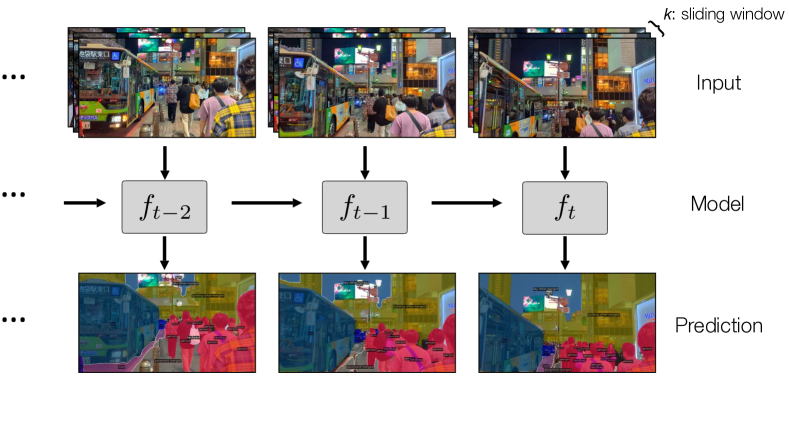
Figure 1: In our streaming setting, the current model $f_{t}$ makes a prediction on the current frame before it can see the next one. The prediction task here is segmentation. $f_{t}$ is obtained through online TTT, initializing from the previous model $f_{t-1}$. A sliding window of size $k$ contains the current and previous frames as test-time training data for the self-supervised task. Concretely, $k=16$ gives a window of only 1.6 seconds in our experiments. Frames taken from COCO Videos, our new dataset.

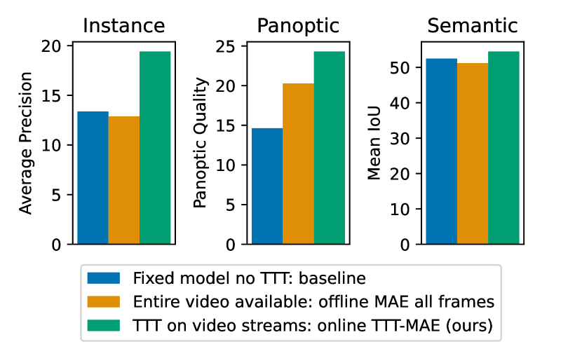
Figure 2: Results for instance and panoptic segmentation on COCO Videos, and semantic segmentation on the KITTI-STEP test set. Online TTT-MAE in the streaming setting achieves the best performance (green) in all tasks. Offline TTT-MAE on all frames (yellow) requires the rather unrealistic setting that makes the entire test video available before making predictions. We think of this as “training on all possible futures”. See more about this method in Subsection 6.1. Online TTT still performs better than offline, by taking advantage of locality.

1 Introduction

Most models in machine learning today are fixed during deployment. As a consequence, a trained model must prepare to be robust to all possible futures. This can be hard because being ready for all futures limits the model’s capacity to be good at any particular one. But only one future actually happens at each moment. The basic idea of test-time training is to continue training on the future once it arrives in the form of a test instance [19, 61]. Since each test instance is observed without a ground truth label, training is performed with self-supervision.

This paper investigates test-time training (TTT) on video streams, where each “future”, or test instance $x_{t}$, is a frame. Naturally, $x_{t}$ and $x_{t+1}$ are visually similar. We are most interested in the intuition discussed above: Is training on the future once it actually happens better than training on all possible futures? More concretely, this question in the streaming setting asks about the role of locality: For making a prediction on $x_{t}$, is it better to perform test-time training offline on all of $x_{1},\dots,x_{T}$ (the video ends at time $T$), or online on only $x_{t}$ (and maybe a few previous frames)?

Our empirical evidence supports locality. The best performance is achieved through online TTT: For each $x_{t}$, only train on itself, and a small window of less than two seconds of frames immediately before $t$. We call this window of frames sliding with $t$ the explicit memory. The optimal explicit memory needs to be short term – in the language of continual learning, some amount of forgetting is actually beneficial. This contrasts with findings in the conventional setting of continual learning [37, 42, 33], but is consistent with recent studies in neuroscience [22].

For online TTT, parameters after training on $x_{t}$ carry over as initialization for training on $x_{t+1}$. We call this the implicit memory. Because such an initialization is usually quite good to begin with, most of the gains from online TTT are realized with only gradient step per frame. Not surprisingly, the effectiveness of both explicit and implicit memory depends on temporal smoothness – the rather general property that $x_{t}$ and $x_{t+1}$ are similar. In Section 6, we conduct ablations on both explicit and implicit memory, and develop a theory based on bias-variance trade-off under smoothness.

Experiments in this paper are also of practical interests, besides conceptual ones. Models for many computer vision tasks are trained with large datasets of still images, e.g. COCO [38] for segmentation, but deployed on video streams. The default is to naively run such models frame-by-frame, since averaging across a sliding window of predictions, a.k.a. temporal smoothing, offers little improvement. Online TTT significantly improves prediction quality on three real-world video datasets, for four tasks: semantic, instance and panoptic segmentation, and colorization. Figure 2 visualizes results for the first three tasks with reliable metrics.

We also collect a new video dataset with dense annotations – COCO Videos. These videos are orders of magnitude longer than in other public datasets, and contain much harder scenes from diverse daily-life scenarios. Longer and more challenging videos better showcase the importance of locality, making it even harder to perform well on all futures at once. The relative improvements on COCO Videos are, respectively, 45% and 66% for instance and panoptic segmentation.

One of the most popular forms of self-supervision in computer vision is image reconstruction: removing parts of the input image, then predicting the removed content [68, 48, 6, 75]. Recently, a class of deep learning models called masked autoencoders (MAE) [27], using reconstruction as the self-supervised task, has been highly influential. TTT-MAE [19] adopts these models for test-time training using reconstruction. The main task in [19] is object recognition. Inspired by the empirical success of TTT-MAE, we make it the inner loop of online TTT, and extend [19] to other main tasks such as segmentation.

Prior work [61] experiments with online TTT (without explicit memory) in the streaming setting, but each $x_{t}$ is drawn independently from the same test distribution. This test distribution is created by adding some synthetic corruption, e.g. Gaussian noise, to a test set of still images, e.g. ImageNet test set [28]. Therefore, all $x_{t}$s belong to the same “future”, and locality is meaningless: TTT on as many $x_{t}$s as possible achieves the best performance by learning to ignore the corruption. TTT on actual video streams is fundamentally different and much more natural.

More recently, [69] also experiments in the streaming setting. While the $x_{t}$s here are not independent, these videos are short clips, again simulated to contain synthetic corruptions, e.g. CityScapes with Artificial Weather. Therefore, like in [61], each corruption moves all $x_{t}$s into almost the same “future”, which they call a domain. Since performance drop is caused by that shared corruption, it is best recovered by training on all $x_{t}$s. Their only dataset without corruptions (CityScapes) sees little improvement (1.4% relative). There is no mentioning of locality, our basic concept of interest.

2 Related Work

2.1 Continual Learning

In the field of continual a.k.a. lifelong learning, a model learns a sequence of tasks in temporal order, and is asked to perform well on all of them [65, 23]. Here is the conventional setting: Each task is defined by a data distribution $P_{t}$, which produces a training set $D^{\text{tr}}_{t}$ and a test set $D^{\text{te}}_{t}$. At each time $t$, the model is evaluated on all the test sets $D^{\text{te}}_{1},\dots,D^{\text{te}}_{t}$ of the past and present, and average performance is reported.

The basic solution is to simply train the model on all of $D^{\text{tr}}_{1},\dots,D^{\text{tr}}_{t}$, which collectively have the same distribution as all the test sets. This is often referred to as the oracle with infinite memory (a.k.a. replay buffer) that remembers everything. However, due to memory constraints, the model at time $t$ is only allowed to train on $D^{\text{tr}}_{t}$. More advanced solutions, therefore, focus on how to retain memory of past data only with model parameters [53, 37, 42, 56, 33, 20].

Some of the literature extends beyond the conventional setting. [1] uses continuous instead of discrete tasks across time. [50] and [17] perform self-supervised learning on unlabeled training sets, and evaluate the learned features on the test sets. [29], [36] and [47] use a labeled training set $D^{\text{tr}}_{0}$ in addition to unlabeled training sets $D^{\text{tr}}_{1},\dots,D^{\text{tr}}_{t}$, connecting with unsupervised domain adaptation. [15] uses alternative metrics, e.g. forward transfer, to justify forgetting for reasons other than computational.

Much of continual learning is motivated by the hope to understand human memory and generalization through the lens of artificial intelligence [26, 13]. Our work shares the same motivation, but focuses on test-time training, without distinct splits of training and test sets.

2.2 Test-Time Training

One of the earliest algorithms for training at test time is Bottou and Vapnik [7]: For each test input, train on its neighbors before making a prediction. Their paper, titled Local Learning, is the first to articulate locality as a basic concept for parametric models in machine learning. This continues to be effective for support vector machines (SVM) [79] and large language models [25]. Another line of work called transductive learning uses test data to add constraints to the margin of SVMs [31, 11, 66]. The principle of transduction, as stated by Vapnik, also emphasizes locality  [18, 67]: "Try to get the answer that you really need but not a more general one."

In computer vision, the idea of training at test time has been well explored for specific applications [30, 57, 46, 73], especially depth estimation [62, 63, 82, 84, 43]. Our paper extends TTT-MAE [19], detailed in Section 3. TTT-MAE, in turn, is inspired by the work Sun et al. [61], which proposed the general framework for test-time training with self-supervision, regardless of application. The particular self-supervised task used in [61] is rotation prediction [21]. Many other papers have followed this framework since then [24, 60, 40, 77], including [69] on videos discussed in Section 1, and [5] which we discuss next.

In [5], each video is treated as a dataset of unordered frames instead of a stream. In particular, there is no concept of past vs. future frames. The same model is used on the entire video. In contrast, our paper emphasizes locality. We have access to only the current and past frames, and our model keeps learning over time. In addition, all of our results are on real world videos, while [5] experiment on videos with artificial corruptions. These corruptions are also i.i.d. across frames.

Our paper is very much inspired by [45]. To make video segmentation more efficient, [45] makes predictions frame-by-frame using a small student model. If the student is not confident, it queries an expensive teacher model, and then trains the student to fit the prediction from the teacher online. Thanks to temporal smoothness, the student can generalize confidently across many frames without querying the teacher, so learning and predicting combined is still faster than naively using the teacher at every frame. Our method only consists of one model, which learns from a self-supervised task instead of a teacher model. Rather than focusing on computational efficiency as in [45], the main goal of our paper is to improve inference quality. Behind their particular algorithm, however, we see the shared idea of locality, regardless of the form of supervision.

3 Background: TTT-MAE

Our paper extends the work of Test-Time Training with Masked Autoencoders (TTT-MAE) [19], and uses TTT-MAE as the inner loop when updating the model for each frame. This section briefly describes TTT-MAE, as background for our extension. Figure 3 illustrates the process of TTT-MAE.

The architecture for TTT with self-supervision [61] is Y-shaped with a stem and two heads: a prediction head $g$ for the self-supervised task, a prediction head $h$ for the main task, and a feature extractor $f$ as the stem. The output features of $f$ are shared between $g$ and $h$ as input. For TTT-MAE, the self-supervised task is masked image reconstruction [27]. Following standard terminology for autoencoders, $f$ is also called the encoder, and $g$ the decoder.

Each input image $x$ is first split into many non-overlapping patches. To produce the autoencoder input $\tilde{x}$, we mask out majority, e.g. 80%, of the patches in $x$ at random. The self-supervised objective $\ell_{s}(g\circ f(\tilde{x}),x)$ compares the reconstructed patches from $g\circ f(\tilde{x})$ to the masked patches in $x$, and computes the pixel-wise mean squared error. For the main task, e.g. segmentation, all patches in the original $x$ are given as input to $h\circ f$, during both training and testing.

3.1 Training-Time Training

There are three widely accepted ways to optimize the model components ($f$, $g$, $h$) at training time: joint training, probing, and fine-tuning. Fine-tuning is unsuitable for TTT, because it makes $h$ rely too much on features that are used by the main task. Our paper uses joint training, described in Section 4. In contrast, [19] uses probing, which we describe next for completeness.

To prepare for probing, the common practice is to first train $f$ and $g$ with $\ell_{s}$ on the training set without ground truth. This preparation stage is also called self-supervised pre-training. TTT-MAE [19] uses the encoder and decoder already pre-trained by [27], denoted by $f_{0}$ and $g_{0}$. During probing, the main task head $h$ is then trained separately by optimizing for $\ell_{m}(h\circ f_{0}(x),y)$, on the training set with ground truth. $f_{0}$ is kept frozen. We denote $h_{0}$ as the main task head after probing. Since $h_{0}$ has been trained for the main task using features from $f_{0}$ as input, $h_{0}\circ f_{0}$ can be directly applied on each test image as a baseline without TTT, keeping the parameters of $f_{0}$ and $h_{0}$ fixed.

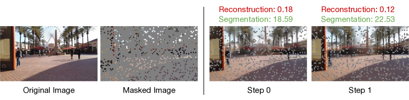
Figure 3: Training a masked autoencoder (MAE) to reconstruct each test image at test time. Reconstructed images on the right visualize the progress of gradient descent on this one-sample learning problem. For each test image, TTT-MAE [19] first masks out majority of the patches. The masked image is given as input to the autoencoder, which then reconstructs those masked patches. The reconstruction loss is the pixel-wise mean squared error between the original and reconstructed patches. Loss on the main task – panoptic segmentation – also falls as reconstruction gets better. The unmasked patches are not shown on the right since they are not part of the reconstruction loss.

3.2 Test-Time Training

At test time, TTT-MAE first takes gradient steps on the following one-sample learning problem:

$$f^{\prime},g^{\prime}=\operatorname*{arg\,min}_{f,g}l_{s}(g\circ f(\tilde{x}^{\prime}),x^{\prime}),$$ (1)

then makes the final prediction $h_{0}\circ f^{\prime}(x^{\prime})$. Crucially, the gradient-based optimization process always starts from $f_{0}$ and $g_{0}$. When evaluating on a test set, TTT-MAE [19] always discards $f^{\prime}$ and $g^{\prime}$ after making a prediction on each test input $x^{\prime}$, and resets the weights back to $f_{0}$ and $g_{0}$ for the next test input. By test-time training on the test inputs independently, we do not assume that they can help each other.

In the original MAE design [27], $g$ is very small relative to $f$, and only the visible patches, e.g. 20%, are processed by $f$. Therefore the overall computational cost of training for the self-supervised task in only a fraction, e.g. $25\%$, of training for the main task. In addition to speeding up training-time training for reconstruction, this reduces the extra test-time cost of TTT-MAE. Each gradient step at test time, counting both forward and backward, costs only half the time of forward prediction for the main task.

4 Test-Time Training on Video Streams

We consider each test video as a smoothly changing sequence of frames $x_{1},\ldots,x_{T}$; time $T$ is when the video ends. In the streaming setting, an algorithm is evaluated on the video following its temporal order, like how a human would consume it. At each time $t$, the algorithm should make a prediction on $x_{t}$ after receiving it from the environment, before seeing any future frame. In addition to $x_{t}$, the past frames $x_{1},\ldots,x_{t-1}$ are also available at time $t$, if the algorithm chooses to use them. Ground truth labels are never given to the algorithm on test videos.

Now we describe our algorithm for this streaming setting. At a high level, our algorithm simply amounts to an outer loop wrapped around TTT-MAE [19]. In practice, making it work involves many design choices.

4.1 Training-Time Training

If there was no self-supervised task, then it is straightforward to simply train $h\circ f$ end-to-end for the main task only. The trained model produced by this process can already be applied on each $x_{t}$ without TTT. We call this baseline Main Task Only in Table 1. However, such a model is not suitable for TTT, since $g$ would have to be trained from scratch at test time.

At training time, our algorithm jointly optimize all three model components in a single stage, end-to-end, on both the self-supervised task and main task. This is called joint training. While joint training was also an option for prior work on TTT-MAE [19], empirical experience at the time indicated that probing (see Section 3) performed better. In this paper, however, we successfully tune joint training to be as effective as probing, and therefore default to joint training because it is simpler than the two-stage process of probing.

Following the notations in Section 3, the self-supervised task loss is denoted by $\ell_{s}$, and the main task loss is $\ell_{m}$. During joint training, we optimize those two losses together to produce a self-supervised task head $g_{0}$, main task head $h_{0}$, and feature extractor $f_{0}$:

$$g_{0},h_{0},f_{0}=\operatorname*{arg\,min}_{g,h,f}\frac{1}{n}\sum_{i=1}^{n}[ \ell_{m}(h\circ f(x_{i}),y_{i})$$

$$+\ell_{s}(g\circ f(\tilde{x}_{i}),x_{i})].$$

The summation is over the training set with $n$ samples, each consisting of input $x_{i}$ and label $y_{i}$. As discussed in Section 3, $\tilde{x}_{i}$ is $x_{i}$ transformed as input for the self-supervised task. In the case of MAE, $\tilde{x}_{i}$ is obtained by masking $80\%$ of the patches in $x_{i}$. Note that although the test instances come from video streams, training-time training uses labeled, still images, e.g. in the COCO training set [38], instead of unlabeled videos.

After joint training, the fixed model $h_{0}\circ f_{0}$ can also be applied directly on each $x_{t}$ without TTT, just like for Main Task Only. We call this new baseline MAE Joint Training. Empirically, we find that these two baselines have roughly the same performance. Joint training does not hurt or help when only considering the fixed model after training-time training.

4.2 Test-Time Training

Another baseline is to blithely apply TTT-MAE by plugging each test frame $x_{t}$ as $x^{\prime}$ into Equation 1, following the process in Section 3. We call this ablated version TTT-MAE No Memory in Table 4. TTT for every $x_{t}$ is initialized with $h_{0}$ and $f_{0}$, by resetting the model parameters back to those after joint training. Like Main Task Only and MAE Joint Training, this ablated version misses the point of using a video. Al three baselines treat each video as a collection of unordered, independent frames that might not contain any information about each other. None of the three can improve over time, no matter how long a video explores the same environment.

Improvement over time is only possible through some form of memory, by retaining information from the past frames $x_{1},\ldots,x_{t-1}$ to help prediction on $x_{t}$. Because evaluation is performed at each timestep only on the current frame, our memory design should favor past data that are most relevant to the present. Fortunately, with the help of nature, the most recent frames usually happen to be the most relevant due to temporal smoothness – observations that are close in time tend to be similar. We design memory that favors recent frames in the following two ways.

Implicit memory. The most natural improvement is to simply not reset the model parameters between timesteps. That is, to initialize test-time training at timestep $t$ with $f_{t-1}$ and $g_{t-1}$, instead of $f_{0}$ and $g_{0}$. This creates an implicit memory, since information carries over from the previous parameters, optimized on previous frames. It also happens to be more biologically plausible: we humans do not constantly reset our minds. In prior work [61], TTT with implicit memory is called the “online” version, in contrast to the “standard” version with reset, for the setting of independent images without temporal smoothness.

Explicit memory. A more explicit way of remembering recent frames is to keep them in a sliding window. Let $k$ denote the window size. At each timestep $t$, our method solves the following optimization problem instead of Equation 1:

$$f_{t},g_{t}=\operatorname*{arg\,min}_{f,g}\frac{1}{k}~{}~{}\sum_{t^{\prime}=t-k+1}^{t}\ell_{s}(g\circ f(\tilde{x}_{t^{\prime}}),x_{t^{\prime}}),$$ (2)

before predicting $h_{0}\circ f_{t}(x_{t})$. Optimization is performed with stochastic gradients: at each iteration, we sample a batch with replacement, uniformly from the same window. Masking is applied independently within and across batches. It turns out that only one iteration is sufficient for our final algorithm, because given temporal smoothness, implicit memory should already provide a good initialization for the optimization problem above.

4.3 Implementation Details

In principle, our method is applicable to any architecture. We use Mask2Former [10], which has achieved state-of-the-art performance on many semantic, instance and panoptic segmentation benchmarks. Our Mask2Former uses a Swin-S [41] backbone – in our case, this is also the shared encoder $f$. Everything following the backbone in the original architecture is taken as the main task head $h$, and our decoder $g$ copies the architecture of $h$ except the last layer that maps into pixel space for reconstruction. Joint training starts from their model checkpoint, which has already been trained for the main task. Only $g$ is initialized from scratch.

Following [27], we split each input into patches, and mask out 80% of them. However, unlike the Vision Transformers [16] used in [27], Swin Transformers use convolutions. Therefore, we must take the entire image as input (with the masked patches in black) instead of only the unmasked patches. Following [48], we use a fourth channel of binaries to indicate if the corresponding input pixels are masked. The model parameters for the fourth channel are initialized from scratch before joint training. If a completely transformer-based architecture for segmentation becomes available in the future, our method would like become even faster, by not encoding the masked patches [27, 19].

Setting	Method	COCO Videos		KITTI-STEP
		Instance	Panoptic	Val.	Test	Time
Independent frames	Main Task Only [10]	13.4	14.6	53.8	52.5	1.8
	MAE Joint Training	13.0	14.4	53.5	52.5	1.8
	TTT-MAE No Mem. [19]	17.2	21.6	53.6	52.5	3.8
Entire video available	Offline MAE All Frames	12.9	20.3	53.2	51.2	-
TTT on video streams	LN Adapt [54]	13.3	15.3	53.8	52.5	2.0
	Tent [70]	13.3	15.2	53.8	52.2	2.8
	Tent Class [70]	13.5	15.3	53.8	52.5	3.7
	Self-Train [69]	-	-	54.7	54.0	6.6
	Self-Train Class [69]	-	-	54.1	53.6	6.9
	Online TTT-MAE (Ours)	19.4	24.3	55.6	54.5	4.1

Table 1: Metrics for instance, panoptic and semantic segmentation are, respectively, average precision (AP), panoptic quality (PQ), and mean IoU (%). Time is in seconds per frame, using a single A100 GPU, averaged over the KITTI-STEP test set. Time costs on COCO Videos are similar, thus omitted for clarity. The self-training baselines are not applicable for instance and panoptic segmentation because the model does not return a confidence per object instance. Bars in Figure 2 correspond to values from the following rows in this table: blue for Main Task Only, yellow for Offline MAE All Frames, and green for Online TTT-MAE (Ours).

5 Results

We experiment with four applications on three real-world datasets: 1) semantic segmentation on KITTI-STEP – a public dataset of urban driving videos; 2) instance and panoptic segmentation on COCO Videos – a new dataset we annotated; 3) colorization on COCO Videos and a collection of black and white films. Please visit our project website at https://video-ttt.github.io/ to watch videos of our results.

5.1 Additional Baselines

In Section 4, we already discussed two baselines using a fixed Mask2Former model without TTT: Main Task Only and MAE Joint Training. We now discuss other baselines. Some of these baselines actually contain our own improvements.

Alternative architectures. The authors of Mask2Former did not evaluated it on KITTI-STEP. We benchmark Mask2Former on the KITTI-STEP validation set against two other popular models of comparable size: SegFormer B4 [74] (64.1M), and DeepLabV3+/RN101 [9] (62.7M), which is used by [69]. Mean IoU are, respectively, 42.0% and 53.1%. Given Main Task Only in Table 1 has 53.8%, we can verify that our pre-trained model (69M) is indeed the state-of-the-art on KITTI-STEP. For COCO segmentation, the authors of Mask2Former have already compared with alternative architectures [10], so we do not repeat their experiments.

Temporal smoothing. We implement temporal smoothing by averaging the predictions across a sliding window, in the same fashion as our explicit memory. The window size is selected to optimize performance after smoothing on the KITTI-STEP validation set. This improves Main Task Only by only 0.4% mean IoU. Applying temporal smoothing to our method also yields 0.3% improvement. This indicates that our method is orthogonal to temporal smoothing. For clarity, we do not use temporal smoothing elsewhere in this paper.

Majority vote with augmentation. We also experiment with test-time augmentation of the input, applying the default data augmentation recipe in the codebase for 100 predictions per frame, then taking the majority vote across predictions as the final output. This improves Main Task Only by 1.2% mean IoU on the KITTI-STEP validation set. Combining the same technique with our method yields roughly the same improvement, indicating that they are again orthogonal. For clarity, we do not use majority vote elsewhere in this paper.

Alternative techniques for TTT. Self-supervision with MAE is only one particular technique for test-time training. Subsection 4.2 describes an outer loop, and any technique that does not use ground truth labels can be used to update the model inside the loop. We experiment with three most promising ones according to prior work: self-training [69], layer norm (LN) adaptation [54], and Tent [70]. For self-training, our implementation significantly improves on the version in [69]. Please refer to Appendix A for an in depth discussion of these three techniques.

Class balancing. Volpi et al. propose a heuristic that is applicable when implicit memory is used [69]: Record the number of predicted classes, for the initial model $h\circ f_{0}$ and the current model $h\circ f_{t}$. Reset the model parameters when the difference is large enough, in which case the predictions of the current model have likely collapsed. To compare with [69], we evaluate this heuristic on self-training and Tent. Methods with class balancing are appended with Class. It cannot be applied to LN Adapt, which does not actually modify the trainable parameters in the model.

Dataset	Len.	Frames	Rate	Cls.
CityScapes-VPS [32]	1.8	3000	17	19
DAVIS [49]	3.5	3455	30	-
YouTube-VOS [76]	4.5	123,467	30	94
KITTI-STEP [72]	40	8,008	10	19
COCO Videos (Ours)	309	30,925	10	134

Table 2: Video datasets with annotations for segmentation. The columns are: average length per video in seconds, total number of frames in the entire dataset, rate in frames per second, and total number of classes. Our videos are orders of magnitude longer, and more diverse in terms of number of classes. COCO Videos is comparable to YouTube-VOS in total duration, taking into account the frame rate. It is much larger than KITTI-STEP in every way.

5.2 Semantic Segmentation on KITTI-STEP

KITTI-STEP [72] contains 9 validation videos and 12 test videos of urban driving scenes. At the rate of 10 frames-per-second, these videos are the longest – up to 106 seconds – among public datasets with dense pixel-wise annotations. All hyper-parameters, even for COCO Videos, are selected on the KITTI-STEP validation set. Joint training is performed on CityScapes [12], another driving dataset with exactly the same 19 categories as KITTI-STEP, but containing still images instead of videos.

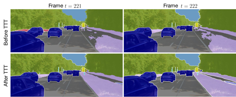
Figure 7: Semantic segmentation predictions for adjacent frames from a video in KITTI-STEP. Top: Results using a fixed model baseline without TTT. Predictions are inconsistent between the two frames. The terrain on the right side of the road is incompletely segmented in both frames, and the terrain on the left is incorrectly classified as a wall on the first frame. Bottom: Results using online TTT-MAE, by the same model, on the same frames as top. Predictions are now consistent and correct.

Table 1 presents our main results. Figure 7 in the appendix visualizes predictions on two frames. Please see project website for more visualizations. Online TTT-MAE in the streaming setting, using both implicit and explicit memory, performs the best. For semantic segmentation, such an improvement is usually considered highly significant in the community.

Baseline techniques that adapt the normalization layers alone do not help at all in these evaluations. This agrees with the evidence in [69]: LN Adapt and Tent help significantly on datasets with synthetic corruptions, but do not help on the real-world dataset (CityScapes).

TTT-MAE optimizes for only 1 iteration per frame, and is 2x slower than the baseline. Comparing with TTT-MAE [19], which optimizes for 20 iterations per image, our method runs much faster. Again, this is because our implicit memory takes advantage of temporal smoothness to get a better initialization for every frame. Resetting parameters is wasteful on videos, because the adjacent frames are very similar.

5.3 COCO Videos

While KITTI-STEP already contains the longest annotated videos among publicly available datasets, they are still far too short for studying long-term phenomenon in locality. KITTI-STEP videos are also limited to driving scenarios, a small subset of the diverse scenarios in our daily lives. These limitations motivate us to collect and annotate our own dataset of videos.

We collected 10 videos, each about 5 minutes, annotated by professionals, in the same format as for COCO instance and panoptic segmentation [38]. The benchmark metrics are also the same as in COCO: average precision (AP) for instance and panoptic quality (PQ) for panoptic. To put things into perspective, each of the 10 videos alone contains more frames, at the same rate, than all of the videos combined in the KITTI-STEP validation set. We compare this new dataset with other publicly available ones in Table 2.

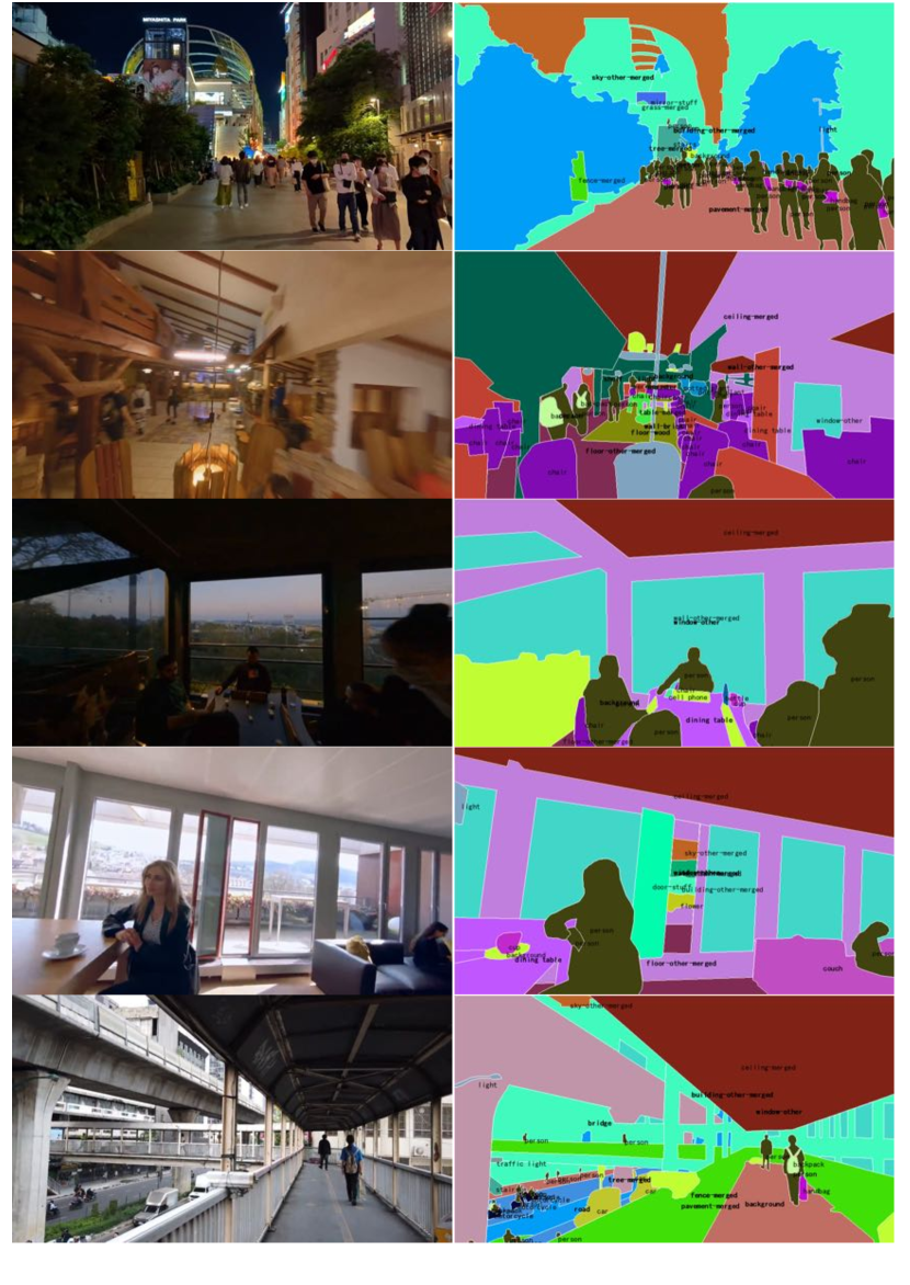
Figure 4: Random frames from COCO Videos (left) and their labels for panoptic segmentation (right).

All videos are egocentric, similar to the visual experience of a human walking around. In particular, they do not follow any tracked object like in Oxford Long-Term Tracking [64] or ImageNet-Vid [55]. Objects leave and enter the camera’s view all the time. Unlike KITTI-STEP and CityScapes that focus on self-driving scenes, our videos are both indoors and outdoors, taken from diverse locations such as sidewalks, markets, schools, offices, restaurants, parks and households. Figure 4 shows random frames from COCO Videos and their ground truth labels.

We start with the publicly available Mask2Former model pre-trained on still images in the COCO training set. Analogous to our procedure for KITTI-STEP, joint training for TTT-MAE is also on COCO images, and our 10 videos are only used for evaluation. Mask2Former is the state-of-the-art on the COCO validation set, with 44.9 AP for instance and 53.6 PQ for panoptic segmentation. But its performance in Table 1 drops to 13.4 AP and 14.6 PQ on COCO Videos. This highlights the challenging nature of COCO Videos, and the fragility of models trained on still images when evaluated on videos in the wild.

We use exactly the same hyper-parameters as tuned on the KITTI-STEP validation set, for all algorithms considered. That is, all of our results for COCO Videos were completed in a single run. As it turns out in Figure 5, using a larger window size would further improve performance. However, we believe such hyper-parameters for TTT should not be tuned on the test videos, so we stick to the window size selected on the KITTI-STEP validation set.

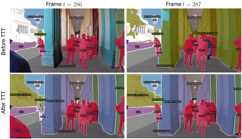
Figure 8: Panoptic segmentation predictions for adjacent frames from a video in our new COCO Videos dataset. Top: Results using a fixed model baseline without TTT. Predictions are inconsistent between the two frames. Bottom: Results using online TTT-MAE, by the same model, on the same frames as top. Predictions are now consistent and correct. Please zoom in to see the instance labels.

Table 1 presents our main results. Figure 8 in the appendix visualizes predictions on two frames. Comparing to Main Task Only, our relative improvements for instance and panoptic segmentation are, respectively, 45% and 66%. Improvements of this magnitude on the state-of-the-art is usually considered dramatic. The self-training baselines are not applicable here because for instance and panoptic segmentation, the model does not return a confidence per object instance.

Interestingly, TTT-MAE No Memory also yields notable improvements on both tasks, and even outperforms Offline MAE All Frames. Intuitively, on the spectrum of locality, Offline MAE All Frames is extremely global, since it tries to be good at all frames for each video. On the other end of the spectrum, TTT-MAE No Memory is the most local, since it only uses information from the current frame. On COCO Videos, local is more helpful than global, if one has to pick an extreme.

Method	FID $\downarrow$	IS $\uparrow$	LPIPS $\uparrow$	PSNR $\uparrow$	SSIM $\uparrow$
Zhang et al. [80]	62.39	5.00 $\pm$ 0.19	0.180	22.27	0.924
Main Task Only [10]	59.96	5.23 $\pm$ 0.12	0.216	20.42	0.881
Online TTT-MAE (Ours)	56.47	5.31 $\pm$ 0.18	0.237	22.97	0.901

Table 3: Results for video colorization on COCO Videos. FID: Fréchet Inception Distance. IS: Inception Score (standard deviation is naturally available). LPIPS: Learned Perceptual Image Patch Similarity. PSNR: Peak Signal-to-Noise Ratio. SSIM: Structural Similarity. Arrows pointing up indicate higher the better, and pointing down indicate lower the better.

5.4 Video Colorization

The goal of colorization is to add realistic RGB colors to gray-scale images  [35, 78]. Our goal here is to demonstrate the generality of online TTT-MAE, not to achieve the state-of-the-art.

Following [80], we simply treat colorization as a supervised learning problem. We use the same architecture as for segmentation – Swin Transformer with two heads, trained on ImageNet [14] to predict the colors given input images processed as gray-scale. We only make the necessary changes to map to a different output space, and do not use domain-specific techniques, e.g., perceptual losses, adversarial learning, and diffusion models. Our bare-minimal baseline already achieves results comparable, if not superior, to those in [80]. Our method uses exactly the same hyper-parameters as for segmentation. All of our colorization experiments were completed in a single run.

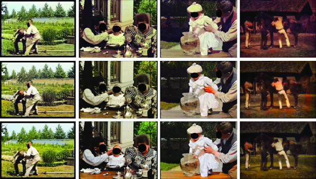
Figure 9: Samples results for video colorization on the Lumiere Brothers films. Top: Using Zhang et al. [80]. Middle: Using our own baseline, Mask2Former with Main Task Only, which is already comparable, if not superior to [80]. Bottom: After applying online TTT-MAE on the baseline. Our colors are more vibrant and consistent within regions.

For quantitative results, we colorize COCO Videos, by processing the 10 videos into black and white. This enables us to compare with the original videos in RGB. Quantitative results are in Table 3. Because colorizing COCO Videos is expensive, we only evaluate our final method and the Main Task Only baseline without TTT. For qualitative results, we also colorize the 10 original black-and-white Lumiere Brothers films from 1895, roughly 40 seconds each, at the rate of 10 frames per second. Figure 9 in Appendix B provides a snapshot of our qualitative results. Please see Appendix B for a list of the films and their lengths.

Our method outperforms the baseline and [80] on all metrics except SSIM. It is a field consensus that PSNR and SSIM often misrepresent actual visual quality because colorization is inherently multi-modal [80, 81], but we still include them for completeness. Please see the project website for the complete set of the original and colorized videos. Our method visually improves the quality in all of them comparing to the baseline, especially in terms of consistency across frames.

6 Analysis on Locality

Now we come back to the two philosophies presented at the beginning of our introduction: training on all possible futures vs. training on the future once it actually happens. In other words, training globally vs. locally. More memory, i.e. larger sliding window, makes training more global, and Offline MAE All Frames takes this to the extreme. The observation that our default method with a small window helps more than Offline MAE or a larger window implies that locality can be beneficial. However, some memory is also better than none, so there seems to be a sweet spot. In this section, we first describe experiments where we make the observations above, then explain the existence of such a sweet spot with theoretical analysis in terms of the bias-variance trade-off.

Method	COCO Videos		KITTI-STEP
	Instance	Panoptic	Val.	Test
TTT-MAE No Mem. [19]	17.2	21.6	53.6	52.5
Implicit Memory Only	18.3	22.7	54.3	54.4
Explicit Memory Only	17.7	21.8	53.6	52.5
Online TTT-MAE (Ours)	19.4	24.3	55.6	54.5

Table 4: Ablations on our two forms of memory. For ease of comparison, the values for TTT-MAE No Memory and Online TTT-MAE (Ours) in Table 1 are reproduced here. The values for Implicit Memory Only match those for window size $k=1$ in Figure 5.

6.1 Empirical Analysis

Table 4 contains ablations on our two forms of memory: implicit and explicit. Both forms of memory contribute to the improved performance of our final method over single-image TTT-MAE [19]. Beyond these basic ablations, we further analyze three aspects of our method.

Offline MAE. Here we describe the process of Offline MAE All Frames, also presented at the beginning of the paper as the yellow bars in Figure 2. It lives in a new setting, where all frames from the entire test video are available for training with the self-supervised task, e.g. MAE, before predictions are made on that video. This provides strictly more information than the streaming setting, where only current and past frames are available. Offline MAE All Frames trains a different model for each test video. The frames are shuffled into a training set, and gradient iterations are taken on batches sampled from this set, in the same way as from the sliding window in Online TTT-MAE. To give Offline MAE All Frames even more unfair advantage, we report results from the best iteration on each test video, as measured by actual test performance, which would not be available in real deployment. For many videos, this best iteration number is around 1000.

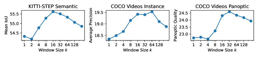
Figure 5: Effect of window size $k$ on performance. The x-axis is in log-scale. The plot for KITTI-STEP is on the validation set, where we selected the optimal hyper-parameter $k=16$. For all three tasks, with a rate of 10 frames per second, 16 frames cover only 1.6 seconds. In simple terms, our algorithm actually prefers a very short-term memory. The optimal $k$ on COCO Videos turns out to be different for both semantic and panoptic segmentation, but the results we report in Table 1 still use $k=16$. For all window sizes, the batch size, and therefore computational cost, is fixed for TTT-MAE.

Window size. The choice of whether to use explicit memory is far from binary. On one end of the spectrum, window size $k=1$ degenerates into not using explicit memory at all. On the other end, $k=\infty$ comes close to Offline MAE All Frames, except the future frames are not trained on since they are not available. Figure 5 analyzes the effect of window size on performance. We observe that too little memory hurts, so does too much. This observation makes intuitive sense: frames in the distant past become less relevant for making a prediction on the current frame, even though they provide more data for TTT. Figure 6 illustrates our intuition.

Temporal smoothness. As discussed in Section 4, temporal smoothness is the key assumption that makes our two forms of memory effective. While this assumption is intuitive, we can test its effect by shuffling all the frames within each video, destroying temporal smoothness, and observing how results change. By construction, all three methods under the setting of independent frames in Table 1 – Main Task Only, MAE Joint Training, and TTT-MAE No Memory – are not affected. The same goes with Offline MAE All Frames, which already shuffles the frames during offline training. For Online TTT-MAE (Ours), however, shuffling hurts performance dramatically. Performance on the KITTI-STEP validation set becomes worse than Main Task Only.

6.2 Theoretical Analysis

To complement our empirical observation that locality can be beneficial, we now rigorously analyze the effect of our window size $k$ for TTT using any self-supervised task.

Notations. We first define the following functions of the shared model parameters $\theta$:

$$\nabla\ell_{m}^{~{}t}(\theta):=\nabla_{\theta}\ell_{m}(x_{t},y_{t};\theta),$$ (3)

$$\nabla\ell_{s}^{~{}t}(\theta):=\nabla_{\theta}\ell_{s}(x_{t};\theta).$$ (4)

These notations are consistent with those in Section 3 and 4, where the main task loss $\ell_{m}$ is defined for object recognition or segmentation, and the self-supervised task loss $\ell_{s}$ instantiates to pixel-wise mean squared error for image reconstruction; $\theta$ refers to parameters for the encoder $f$.

Problem statement. Taking gradient steps with $\nabla\ell_{m}^{~{}t}$ directly optimizes the test loss, since $y_{t}$ is the ground truth label of test input $x_{t}$. However, $y_{t}$ is not available, so TTT optimizes the self-supervised loss $\ell_{s}$ instead. Among the available gradients, $\nabla\ell_{s}^{~{}t}$ is the most relevant. But we also have the past inputs $x_{1},\dots,x_{t-1}$. Should we use some, or even all of them?

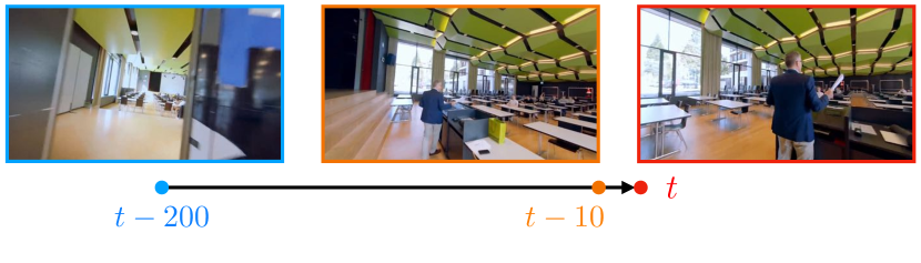
Figure 6: An illustration of the principle of locality in video streams. Our goal is improve prediction on the current frame, shot inside a lecture hall. The frame at $t-10$ was still inside this hall. Including it in our sliding window decreases variance for TTT. However, the frame at $t-200$ was shot before entering the hall. Including it would significantly increase bias, because it is no longer relevant to the current frame. Frames taken from COCO Videos.

Theorem. For every timestep $t$, consider TTT with gradient-based optimization using:

$$\frac{1}{k}\sum_{t^{\prime}=t-k+1}^{t}\nabla\ell_{s}^{~{}t^{\prime}},$$ (5)

where $k$ is the window size. Let $\theta_{0}$ denote the initial condition, and $\tilde{\theta}$ where optimization converges for TTT. Let $\theta^{*}$ denote the optimal solution of $\ell_{m}^{~{}t}$ in the local neighborhood of $\theta_{0}$. Then we have

$$\mathop{\mathbb{E}}\left[\ell_{m}(x_{t},y_{t};\tilde{\theta})-\ell_{m}(x_{t},y_{t};\theta^{*})\right]\leq\frac{1}{2\alpha}\left(k^{2}\beta^{2}\eta^{2}+\frac{1}{k}\sigma^{2}\right),$$

under the following three assumptions:

1. In a local neighborhood of $\theta^{*}$, $\ell_{m}^{~{}t}$ is $\alpha$-strongly convex in $\theta$, and $\beta$-smooth in $x$.

2. $\|x_{t+1}-x_{t}\|\leq\eta$.

3. $\nabla\ell_{m}^{~{}t}=\nabla\ell_{s}^{~{}t}+\delta_{t}$, where $\delta_{t}$ is a random variable with mean zero and variance $\sigma^{2}$.

The proof is in Appendix C.

Remark on assumptions. Assumption 1, that neural networks are strongly convex around their local minima, is widely accepted in the deep learning theory community [2, 83, 71]. Assumption 2 is simply temporal smoothness in L2 norm; any norm could be used here as long as the norm in Assumption 1 for strong convexity is also changed accordingly. Assumption 3, that the main task and self-supervised task have correlated gradients, comes from the theoretical analysis of [61].

Bias-variance trade-off. Disregarding the constant factor of $1/\alpha$, the upper bound in Theorem 1 is the sum of two terms: $k^{2}\beta^{2}\eta^{2}$ and $1/k\cdot\sigma^{2}$. The former is the bias term, growing with $\eta$. The latter is the variance term, growing with $\sigma^{2}$. More memory, i.e., sliding window with larger size $k$, reduces variance, but increases bias. This is consistent with our intuition in Figure 6. Optimizing this upper bound w.r.t. $k$ shows the theoretical sweet spot to occur at

$$k=\left(\frac{\sigma^{2}}{\beta^{2}\eta^{2}}\right)^{1/3}.$$

7 Discussion

In the end, we connect our findings to other concepts of machine learning, with the hope of inspiring further discussion.

Unsupervised domain adaptation. The setting of Offline MAE All Frames, that the entire unlabeled test video is available at once, is very similar to unsupervised domain adaptation (UDA). Each test video can be viewed as a target domain, and offline MAE practically treats the frames as i.i.d. data drawn from a single distribution. The only difference with UDA is that the unlabeled video serves as both training and test data. In fact, this slightly modified version of the UDA setting is sometimes called test-time adaptation. Our results suggest that this perspective of seeing each video as a target domain might be misleading for algorithm design, because it discourages locality.

Continual learning. Conventional wisdom in the continual learning community believes that forgetting is harmful. Specifically, the best accuracy is achieved by remembering everything with an infinite replay buffer, given unlimited computer memory. Our streaming setting is different from those commonly studied by the continual learning community, because it does not have distinct splits of training and test sets, as explained in Subsection 2.1. However, our sliding window can be viewed as a replay buffer, and limiting its size can be viewed as a form of forgetting. In this context, our results suggest that forgetting can actually be beneficial.

Test-time training on nearest neighbors (TTT-NN). Here is an alternative heuristic for test-time training: For each test instance, retrieve its nearest neighbors from the training set, and fine-tune the model on those neighbors before applying it to the test instance. As discussed in Subsection 2.2, this simple heuristic has been shown to significantly improve prediction quality in [7] three decades ago, and more recently in [25] for large language models. Given temporal smoothness, our sliding window can be seen as retrieving neighbors of the current frame. The only difference is that our method retrieves from past unlabeled test instances, while TTT-NN retrieves from labeled training data. Therefore, our method must use self-supervision for TTT, instead of supervised learning on the neighbors as in TTT-NN. But this difference also implies an important advantage for our method: Given temporal smoothness, our neighbors will always be actually relevant, while the neighbors from the training set might not.

Appendix A Baseline Techniques for TTT

A.1 Self-Training

Self-training is a popular technique in semi-supervised learning [51, 52, 85, 4, 3] and domain adaptation [34, 86, 44, 39, 59]. It is also evaluated in [69], but is shown to produce inferior performance. We experiment with both its original form, and our own designs that actually improve this baseline.

We assume that for each test image $x$, the prediction $\hat{y}$ is also of the same shape in 2D, which is true in semantic segmentation and colorization. We also assume that $F$ outputs a estimated confidence map $\hat{c}$ of the same shape as $\hat{y}$. Specifically, for pixel $x[i,j]$, $\hat{y}[i,j]$ is the predicted class of this pixel, and $\hat{c}[i,j]$ is the estimated confidence of $\hat{y}[i,j]$.

Self-training repeats many iterations of the following:

• Start with an empty set of labels $D$ for this iteration.

• Loop over every $[i,j]$ location, add pseudo-label $\hat{y}[i,j]$ to $D$ if $\hat{c}[i,j]>\lambda$, for a fixed threshold $\lambda$.

• Train $F$ to fit this iteration’s set $D$, as if the selected pseudo-labels are ground truth labels.

Our first design improvement is incorporating the confidence threshold $\lambda$. In [69], all predictions are pseudo-labels, regardless of confidence. Experiments show that for low $\lambda$, or with $\lambda=0$ in [69], self-training is noisy and unstable, as expected.

However, for high $\lambda$, there is limited learning signal, e.g. little gradient, since $f$ is already very confident about the pseudo-label. Our second design improvement, inspired by [58], is to make learning more challenging with an already confident prediction, by masking image patches in $x$. In [58], masking is applied sparingly on 2.5% of the pixels in average. We mask 80% of the pixels, inspired by [27].

A.2 Layer Norm Adapt

Prior work [54] shows that simply recalculating the batch normalization (BN) statistics works well for unsupervised domain adaptation. [69] applies this technique to video streams by accumulating the statistics with a forward pass on each frame once it is revealed. Since modern transformers use layer normalization (LN) instead, we apply the same technique to LN.

A.3 Tent

The normalization layers (BN and LN) also contain trainable parameters that modify the statistics. Optimizing those parameters requires a self-supervised objective. Tent [70] is an objective for learning only those parameters at test time, by minimizing the softmax entropy of the predicted distribution over classes. We update the LN statistics and parameters with Tent, in the same loop as our method, also using implicit and explicit memory. Hyper-parameters are searched on the KITTI-STEP validation set to be optimal for Tent.

Appendix B Colorization Dataset - Lumière Brothers Films

We provide results on the following 10 Lumiere Brothers films, all in the public domain:

1. Workers Leaving the Lumiere Factory (46 s)

2. The Gardener (49 s)

3. The Disembarkment of the Congress of Photographers in Lyon (48 s)

4. Horse Trick Riders (46 s)

5. Fishing for Goldfish (42 s)

6. Blacksmiths (49 s)

7. Baby’s Meal (41 s)

8. Jumping Onto the Blanket (41 s)

9. Cordeliers Square in Lyon (44 s)

10. The Sea (38 s)

Appendix C Proof of Theorem 1

We first prove the following lemma.

Lemma. Let $f:\mathbb{R}^{n}\rightarrow\mathbb{R}$ be $\alpha$-strongly convex and continuously differentiable, and denote its optimal solution as $x^{*}$. Let

$$\tilde{f}(x)=f(x)+v^{T}x,$$ (6)

and denote its optimal solution as $\tilde{x}^{*}$. Then

$$f(\tilde{x}^{*})-f(x^{*})\leq\frac{1}{2\alpha}\|v\|^{2}.$$ (7)

Proof of lemma. It is a well known fact in convex optimization [8] that for $f$ $\alpha$-strongly convex and continuously differentiable,

$$\alpha(f(x)-f(x^{*}))\leq\frac{1}{2}\|\nabla f(x)\|^{2},$$ (8)

for all $x$. Since $\tilde{x}^{*}$ is the optimal solution of $\tilde{f}$ and $\tilde{f}$ is also convex, we have $\nabla\tilde{f}(\tilde{x}^{*})=0$. But

$$\nabla\tilde{f}(x)=\nabla f(x)+v,$$ (9)

so we then have

$$\nabla f(\tilde{x}^{*})=\nabla\tilde{f}(\tilde{x}^{*})-v=-v.$$ (10)

Make $x=\tilde{x}^{*}$ in Equation 8, we finish the proof.

Proof of theorem. By Assumptions 1 and 2, we have

$$\|\nabla\ell_{m}^{~{}t}(\theta)-\nabla\ell_{m}^{~{}t-1}(\theta)\|\leq\beta\eta.$$ (11)

$$\frac{1}{k}\sum_{t^{\prime}=t-k+1}^{t}\nabla\ell_{s}^{~{}t^{\prime}} =\frac{1}{k}\sum_{t^{\prime}=t-k+1}^{t}\nabla\ell_{m}^{~{}t^{\prime}}+\frac{1}{k}\sum_{t^{\prime}=t-k+1}^{t}\delta_{t^{\prime}}$$ (12)

$$=\frac{1}{k}\sum_{t^{\prime}=t-k+1}^{t}\left[\nabla\ell_{m}^{~{}t}+\sum_{t^{\prime\prime}=t^{\prime}}^{t-1}\left(\nabla\ell_{m}^{~{}t^{\prime\prime}}-\nabla\ell_{m}^{~{}t^{\prime\prime}+1}\right)\right]+\frac{1}{k}\sum_{t^{\prime}=t-k+1}^{t}\delta_{t^{\prime}}$$ (13)

$$=\nabla\ell_{m}^{~{}t}+\frac{1}{k}\left[~{}\sum_{t^{\prime}=t-k+1}^{t}\sum_{t^{\prime\prime}=t^{\prime}}^{t-1}\left(\nabla\ell_{m}^{~{}t^{\prime\prime}}-\nabla\ell_{m}^{~{}t^{\prime\prime}+1}\right)+\sum_{t^{\prime}=t-k+1}^{t}\delta_{t^{\prime}}~{}\right]$$ (14)

To simplify notations, define

$$A =\sum_{t^{\prime}=t-k+1}^{t}\sum_{t^{\prime\prime}=t^{\prime}}^{t-1}\left(\nabla\ell_{m}^{~{}t^{\prime\prime}}-\nabla\ell_{m}^{~{}t^{\prime\prime}+1}\right),$$ (15)

$$B =\sum_{t^{\prime}=t-k+1}^{t}\delta_{t^{\prime}}.$$ (16)

So

$$\frac{1}{k}\sum_{t^{\prime}=t-k+1}^{t}\nabla\ell_{s}^{~{}t^{\prime}}-\nabla\ell_{m}^{~{}t}=(A+B)/k.$$ (17)

Because $\ell_{m}^{~{}t}$ is convex in $\theta$, we know that taking gradient steps with $\nabla\ell_{m}^{~{}t}$ would eventually reach the local optima of $\ell_{m}^{~{}t}$. Because $\frac{1}{k}\sum_{t^{\prime}=t-k+1}^{t}\nabla\ell_{s}^{~{}t^{\prime}}$ differs from $\nabla\ell_{m}^{~{}t}$ by $(A+B)/k$, we know that taking gradient steps with the former reaches the local optima of $\ell_{m}^{~{}t}+(A+B)\theta/2$. Now we can invoke our lemma. To do so, we first calculate

$$\mathop{\mathbb{E}}\bigg{\|}\frac{1}{k}\sum_{t^{\prime}=t-k+1}^{t}\nabla\ell_{s}^{~{}t^{\prime}}-\nabla\ell_{m}^{~{}t}\bigg{\|}^{2} =\frac{1}{k^{2}}\mathop{\mathbb{E}}\|A+B\|^{2}$$ (18)

$$=\frac{1}{k^{2}}\left(\|A\|^{2}+\mathop{\mathbb{E}}\|B\|^{2}+\mathop{\mathbb{E}}A^{T}B\right)$$ (19)

$$\leq\frac{1}{k^{2}}\left(k^{4}\beta^{2}\eta^{2}+k\sigma^{2}\right)$$ (20)

$$=k^{2}\beta^{2}\eta^{2}+\frac{1}{k}\sigma^{2}.$$ (21)

Then by our lemma, we have

$$\mathop{\mathbb{E}}\left[\ell_{m}(x_{t},y_{t};\tilde{\theta})-\ell_{m}^{*}\right]\leq\frac{1}{2\alpha}\mathop{\mathbb{E}}\bigg{\|}\frac{1}{k}\sum_{t^{\prime}=t-k+1}^{t}\nabla\ell_{s}^{~{}t^{\prime}}-\nabla\ell_{m}^{~{}t}\bigg{\|}^{2}\leq\frac{1}{2\alpha}\left(k^{2}\beta^{2}\eta^{2}+\frac{1}{k}\sigma^{2}\right).$$ (22)

This finishes the proof.

References

- [1] Rahaf Aljundi, Klaas Kelchtermans, and Tinne Tuytelaars. Task-free continual learning. In Proceedings of the IEEE/CVF Conference on Computer Vision and Pattern Recognition, pages 11254–11263, 2019.
- [2] Zeyuan Allen-Zhu, Yuanzhi Li, and Zhao Song. A convergence theory for deep learning via over-parameterization. In Kamalika Chaudhuri and Ruslan Salakhutdinov, editors, Proceedings of the 36th International Conference on Machine Learning, volume 97 of Proceedings of Machine Learning Research, pages 242–252. PMLR, 09–15 Jun 2019.
- [3] Yuki Asano, Mandela Patrick, Christian Rupprecht, and Andrea Vedaldi. Labelling unlabelled videos from scratch with multi-modal self-supervision. Advances in Neural Information Processing Systems, 33:4660–4671, 2020.
- [4] Yuki Markus Asano, Christian Rupprecht, and Andrea Vedaldi. Self-labelling via simultaneous clustering and representation learning. arXiv preprint arXiv:1911.05371, 2019.
- [5] Fatemeh Azimi, Sebastian Palacio, Federico Raue, Jörn Hees, Luca Bertinetto, and Andreas Dengel. Self-supervised test-time adaptation on video data. In Proceedings of the IEEE/CVF Winter Conference on Applications of Computer Vision, pages 3439–3448, 2022.
- [6] Hangbo Bao, Li Dong, and Furu Wei. Beit: BERT pre-training of image transformers. CoRR, abs/2106.08254, 2021.
- [7] Léon Bottou and Vladimir Vapnik. Local learning algorithms. Neural computation, 4(6):888–900, 1992.
- [8] Sébastien Bubeck et al. Convex optimization: Algorithms and complexity. Foundations and Trends® in Machine Learning, 8(3-4):231–357, 2015.
- [9] Liang-Chieh Chen, George Papandreou, Florian Schroff, and Hartwig Adam. Rethinking atrous convolution for semantic image segmentation. arXiv preprint arXiv:1706.05587, 2017.
- [10] Bowen Cheng, Ishan Misra, Alexander G Schwing, Alexander Kirillov, and Rohit Girdhar. Masked-attention mask transformer for universal image segmentation. arXiv preprint arXiv:2112.01527, 2021.
- [11] Ronan Collobert, Fabian Sinz, Jason Weston, Léon Bottou, and Thorsten Joachims. Large scale transductive svms. Journal of Machine Learning Research, 7(8), 2006.
- [12] Marius Cordts, Mohamed Omran, Sebastian Ramos, Timo Rehfeld, Markus Enzweiler, Rodrigo Benenson, Uwe Franke, Stefan Roth, and Bernt Schiele. The cityscapes dataset for semantic urban scene understanding. In Proceedings of the IEEE conference on computer vision and pattern recognition, pages 3213–3223, 2016.
- [13] Matthias De Lange, Rahaf Aljundi, Marc Masana, Sarah Parisot, Xu Jia, Aleš Leonardis, Gregory Slabaugh, and Tinne Tuytelaars. A continual learning survey: Defying forgetting in classification tasks. IEEE transactions on pattern analysis and machine intelligence, 44(7):3366–3385, 2021.
- [14] Jia Deng, Wei Dong, Richard Socher, Li-Jia Li, Kai Li, and Li Fei-Fei. Imagenet: A large-scale hierarchical image database. In 2009 IEEE conference on computer vision and pattern recognition, pages 248–255. Ieee, 2009.
- [15] Natalia Díaz-Rodríguez, Vincenzo Lomonaco, David Filliat, and Davide Maltoni. Don’t forget, there is more than forgetting: new metrics for continual learning. arXiv preprint arXiv:1810.13166, 2018.
- [16] Alexey Dosovitskiy, Lucas Beyer, Alexander Kolesnikov, Dirk Weissenborn, Xiaohua Zhai, Thomas Unterthiner, Mostafa Dehghani, Matthias Minderer, Georg Heigold, Sylvain Gelly, et al. An image is worth 16x16 words: Transformers for image recognition at scale. arXiv preprint arXiv:2010.11929, 2020.
- [17] Enrico Fini, Victor G Turrisi da Costa, Xavier Alameda-Pineda, Elisa Ricci, Karteek Alahari, and Julien Mairal. Self-supervised models are continual learners. In Proceedings of the IEEE/CVF Conference on Computer Vision and Pattern Recognition, pages 9621–9630, 2022.
- [18] A. Gammerman, V. Vovk, and V. Vapnik. Learning by transduction. In In Uncertainty in Artificial Intelligence, pages 148–155. Morgan Kaufmann, 1998.
- [19] Yossi Gandelsman, Yu Sun, Xinlei Chen, and Alexei A. Efros. Test-time training with masked autoencoders. Advances in Neural Information Processing Systems, 2022.
- [20] Spyros Gidaris and Nikos Komodakis. Dynamic few-shot visual learning without forgetting. In Proceedings of the IEEE Conference on Computer Vision and Pattern Recognition, pages 4367–4375, 2018.
- [21] Spyros Gidaris, Praveer Singh, and Nikos Komodakis. Unsupervised representation learning by predicting image rotations. arXiv preprint arXiv:1803.07728, 2018.
- [22] Lauren Gravitz. The importance of forgetting. Nature, 571(July):S12–S14, 2019.
- [23] Raia Hadsell, Dushyant Rao, Andrei A Rusu, and Razvan Pascanu. Embracing change: Continual learning in deep neural networks. Trends in cognitive sciences, 24(12):1028–1040, 2020.
- [24] Nicklas Hansen, Rishabh Jangir, Yu Sun, Guillem Alenyà, Pieter Abbeel, Alexei A Efros, Lerrel Pinto, and Xiaolong Wang. Self-supervised policy adaptation during deployment. arXiv preprint arXiv:2007.04309, 2020.
- [25] Moritz Hardt and Yu Sun. Test-time training on nearest neighbors for large language models. arXiv preprint arXiv:2305.18466, 2023.
- [26] Demis Hassabis, Dharshan Kumaran, Christopher Summerfield, and Matthew Botvinick. Neuroscience-inspired artificial intelligence. Neuron, 95(2):245–258, 2017.
- [27] Kaiming He, Xinlei Chen, Saining Xie, Yanghao Li, Piotr Dollár, and Ross B. Girshick. Masked autoencoders are scalable vision learners. CoRR, abs/2111.06377, 2021.
- [28] Dan Hendrycks and Thomas G. Dietterich. Benchmarking neural network robustness to common corruptions and perturbations. CoRR, abs/1903.12261, 2019.
- [29] Judy Hoffman, Trevor Darrell, and Kate Saenko. Continuous manifold based adaptation for evolving visual domains. In Proceedings of the IEEE Conference on Computer Vision and Pattern Recognition, pages 867–874, 2014.
- [30] Vidit Jain and Erik Learned-Miller. Online domain adaptation of a pre-trained cascade of classifiers. In CVPR 2011, pages 577–584. IEEE, 2011.
- [31] Thorsten Joachims. Learning to classify text using support vector machines, volume 668. Springer Science & Business Media, 2002.
- [32] Dahun Kim, Sanghyun Woo, Joon-Young Lee, and In So Kweon. Video panoptic segmentation. In Proceedings of the IEEE/CVF Conference on Computer Vision and Pattern Recognition, pages 9859–9868, 2020.
- [33] James Kirkpatrick, Razvan Pascanu, Neil Rabinowitz, Joel Veness, Guillaume Desjardins, Andrei A Rusu, Kieran Milan, John Quan, Tiago Ramalho, Agnieszka Grabska-Barwinska, et al. Overcoming catastrophic forgetting in neural networks. Proceedings of the national academy of sciences, 114(13):3521–3526, 2017.
- [34] Ananya Kumar, Tengyu Ma, and Percy Liang. Understanding self-training for gradual domain adaptation. In International Conference on Machine Learning, pages 5468–5479. PMLR, 2020.
- [35] Chenyang Lei and Qifeng Chen. Fully automatic video colorization with self-regularization and diversity. In Proceedings of the IEEE/CVF Conference on Computer Vision and Pattern Recognition, pages 3753–3761, 2019.
- [36] Da Li and Timothy Hospedales. Online meta-learning for multi-source and semi-supervised domain adaptation. In European Conference on Computer Vision, pages 382–403. Springer, 2020.
- [37] Zhizhong Li and Derek Hoiem. Learning without forgetting. IEEE transactions on pattern analysis and machine intelligence, 40(12):2935–2947, 2017.
- [38] Tsung-Yi Lin, Michael Maire, Serge Belongie, James Hays, Pietro Perona, Deva Ramanan, Piotr Dollár, and C Lawrence Zitnick. Microsoft coco: Common objects in context. In European conference on computer vision, pages 740–755. Springer, 2014.
- [39] Xiaofeng Liu, Bo Hu, Xiongchang Liu, Jun Lu, Jane You, and Lingsheng Kong. Energy-constrained self-training for unsupervised domain adaptation. In 2020 25th International Conference on Pattern Recognition (ICPR), pages 7515–7520. IEEE, 2021.
- [40] Yuejiang Liu, Parth Kothari, Bastien van Delft, Baptiste Bellot-Gurlet, Taylor Mordan, and Alexandre Alahi. Ttt++: When does self-supervised test-time training fail or thrive? Advances in Neural Information Processing Systems, 34, 2021.
- [41] Ze Liu, Yutong Lin, Yue Cao, Han Hu, Yixuan Wei, Zheng Zhang, Stephen Lin, and Baining Guo. Swin transformer: Hierarchical vision transformer using shifted windows. In Proceedings of the IEEE/CVF International Conference on Computer Vision, pages 10012–10022, 2021.
- [42] David Lopez-Paz and Marc’Aurelio Ranzato. Gradient episodic memory for continual learning. In Advances in Neural Information Processing Systems, pages 6467–6476, 2017.
- [43] Xuan Luo, Jia-Bin Huang, Richard Szeliski, Kevin Matzen, and Johannes Kopf. Consistent video depth estimation. ACM Transactions on Graphics (ToG), 39(4):71–1, 2020.
- [44] Ke Mei, Chuang Zhu, Jiaqi Zou, and Shanghang Zhang. Instance adaptive self-training for unsupervised domain adaptation. In European conference on computer vision, pages 415–430. Springer, 2020.
- [45] Ravi Teja Mullapudi, Steven Chen, Keyi Zhang, Deva Ramanan, and Kayvon Fatahalian. Online model distillation for efficient video inference. arXiv preprint arXiv:1812.02699, 2018.
- [46] Yotam Nitzan, Kfir Aberman, Qiurui He, Orly Liba, Michal Yarom, Yossi Gandelsman, Inbar Mosseri, Yael Pritch, and Daniel Cohen-Or. Mystyle: A personalized generative prior. arXiv preprint arXiv:2203.17272, 2022.
- [47] Theodoros Panagiotakopoulos, Pier Luigi Dovesi, Linus Härenstam-Nielsen, and Matteo Poggi. Online domain adaptation for semantic segmentation in ever-changing conditions. arXiv preprint arXiv:2207.10667, 2022.
- [48] Deepak Pathak, Philipp Krahenbuhl, Jeff Donahue, Trevor Darrell, and Alexei A Efros. Context encoders: Feature learning by inpainting. In Proceedings of the IEEE conference on computer vision and pattern recognition, pages 2536–2544, 2016.
- [49] Jordi Pont-Tuset, Federico Perazzi, Sergi Caelles, Pablo Arbeláez, Alexander Sorkine-Hornung, and Luc Van Gool. The 2017 davis challenge on video object segmentation. arXiv:1704.00675, 2017.
- [50] Senthil Purushwalkam, Pedro Morgado, and Abhinav Gupta. The challenges of continuous self-supervised learning. arXiv preprint arXiv:2203.12710, 2022.
- [51] Ilija Radosavovic, Piotr Dollár, Ross Girshick, Georgia Gkioxari, and Kaiming He. Data distillation: Towards omni-supervised learning. In Proceedings of the IEEE Conference on Computer Vision and Pattern Recognition (CVPR), June 2018.
- [52] Chuck Rosenberg, Martial Hebert, and Henry Schneiderman. Semi-supervised self-training of object detection models. arXiv, 2005.
- [53] Adam Santoro, Sergey Bartunov, Matthew Botvinick, Daan Wierstra, and Timothy Lillicrap. Meta-learning with memory-augmented neural networks. In International conference on machine learning, pages 1842–1850, 2016.
- [54] Steffen Schneider, Evgenia Rusak, Luisa Eck, Oliver Bringmann, Wieland Brendel, and Matthias Bethge. Improving robustness against common corruptions by covariate shift adaptation. Advances in Neural Information Processing Systems, 33:11539–11551, 2020.
- [55] Vaishaal Shankar, Achal Dave, Rebecca Roelofs, Deva Ramanan, Benjamin Recht, and Ludwig Schmidt. Do image classifiers generalize across time? In Proceedings of the IEEE/CVF International Conference on Computer Vision, pages 9661–9669, 2021.
- [56] Hanul Shin, Jung Kwon Lee, Jaehong Kim, and Jiwon Kim. Continual learning with deep generative replay. Advances in neural information processing systems, 30, 2017.
- [57] Assaf Shocher, Nadav Cohen, and Michal Irani. “zero-shot” super-resolution using deep internal learning. In Proceedings of the IEEE Conference on Computer Vision and Pattern Recognition, pages 3118–3126, 2018.
- [58] Kihyuk Sohn, Zizhao Zhang, Chun-Liang Li, Han Zhang, Chen-Yu Lee, and Tomas Pfister. A simple semi-supervised learning framework for object detection. arXiv preprint arXiv:2005.04757, 2020.
- [59] Teo Spadotto, Marco Toldo, Umberto Michieli, and Pietro Zanuttigh. Unsupervised domain adaptation with multiple domain discriminators and adaptive self-training. In 2020 25th International Conference on Pattern Recognition (ICPR), pages 2845–2852. IEEE, 2021.
- [60] Yu Sun, Wyatt L Ubellacker, Wen-Loong Ma, Xiang Zhang, Changhao Wang, Noel V Csomay-Shanklin, Masayoshi Tomizuka, Koushil Sreenath, and Aaron D Ames. Online learning of unknown dynamics for model-based controllers in legged locomotion. IEEE Robotics and Automation Letters, 6(4):8442–8449, 2021.
- [61] Yu Sun, Xiaolong Wang, Zhuang Liu, John Miller, Alexei Efros, and Moritz Hardt. Test-time training with self-supervision for generalization under distribution shifts. In International Conference on Machine Learning, pages 9229–9248. PMLR, 2020.
- [62] Alessio Tonioni, Oscar Rahnama, Thomas Joy, Luigi Di Stefano, Thalaiyasingam Ajanthan, and Philip HS Torr. Learning to adapt for stereo. In Proceedings of the IEEE/CVF Conference on Computer Vision and Pattern Recognition, pages 9661–9670, 2019.
- [63] Alessio Tonioni, Fabio Tosi, Matteo Poggi, Stefano Mattoccia, and Luigi Di Stefano. Real-time self-adaptive deep stereo. In Proceedings of the IEEE/CVF Conference on Computer Vision and Pattern Recognition, pages 195–204, 2019.
- [64] Jack Valmadre, Luca Bertinetto, Joao F Henriques, Ran Tao, Andrea Vedaldi, Arnold WM Smeulders, Philip HS Torr, and Efstratios Gavves. Long-term tracking in the wild: A benchmark. In Proceedings of the European conference on computer vision (ECCV), pages 670–685, 2018.
- [65] Gido M Van de Ven and Andreas S Tolias. Three scenarios for continual learning. arXiv preprint arXiv:1904.07734, 2019.
- [66] Vladimir Vapnik. The nature of statistical learning theory. Springer science & business media, 2013.
- [67] Vladimir Vapnik and S. Kotz. Estimation of Dependences Based on Empirical Data: Empirical Inference Science (Information Science and Statistics). Springer-Verlag, Berlin, Heidelberg, 2006.
- [68] Pascal Vincent, Hugo Larochelle, Yoshua Bengio, and Pierre-Antoine Manzagol. Extracting and composing robust features with denoising autoencoders. In ICML, page 1096–1103, 2008.
- [69] Riccardo Volpi, Pau De Jorge, Diane Larlus, and Gabriela Csurka. On the road to online adaptation for semantic image segmentation. In Proceedings of the IEEE/CVF Conference on Computer Vision and Pattern Recognition, pages 19184–19195, 2022.
- [70] Dequan Wang, Evan Shelhamer, Shaoteng Liu, Bruno Olshausen, and Trevor Darrell. Tent: Fully test-time adaptation by entropy minimization. arXiv preprint arXiv:2006.10726, 2020.
- [71] Yifei Wang, Jonathan Lacotte, and Mert Pilanci. The hidden convex optimization landscape of regularized two-layer relu networks: an exact characterization of optimal solutions. In International Conference on Learning Representations, 2021.
- [72] Mark Weber, Jun Xie, Maxwell Collins, Yukun Zhu, Paul Voigtlaender, Hartwig Adam, Bradley Green, Andreas Geiger, Bastian Leibe, Daniel Cremers, et al. Step: Segmenting and tracking every pixel. arXiv preprint arXiv:2102.11859, 2021.
- [73] Binhui Xie, Shuang Li, Mingjia Li, Chi Harold Liu, Gao Huang, and Guoren Wang. Sepico: Semantic-guided pixel contrast for domain adaptive semantic segmentation. IEEE Transactions on Pattern Analysis and Machine Intelligence, 2023.
- [74] Enze Xie, Wenhai Wang, Zhiding Yu, Anima Anandkumar, Jose M Alvarez, and Ping Luo. Segformer: Simple and efficient design for semantic segmentation with transformers. Advances in Neural Information Processing Systems, 34, 2021.
- [75] Zhenda Xie, Zheng Zhang, Yue Cao, Yutong Lin, Jianmin Bao, Zhuliang Yao, Qi Dai, and Han Hu. Simmim: A simple framework for masked image modeling. In International Conference on Computer Vision and Pattern Recognition (CVPR), 2022.
- [76] Ning Xu, Linjie Yang, Yuchen Fan, Jianchao Yang, Dingcheng Yue, Yuchen Liang, Brian Price, Scott Cohen, and Thomas Huang. Youtube-vos: Sequence-to-sequence video object segmentation. In Proceedings of the European conference on computer vision (ECCV), pages 585–601, 2018.
- [77] Longhui Yuan, Binhui Xie, and Shuang Li. Robust test-time adaptation in dynamic scenarios. In Proceedings of the IEEE/CVF Conference on Computer Vision and Pattern Recognition, pages 15922–15932, 2023.
- [78] Bo Zhang, Mingming He, Jing Liao, Pedro V Sander, Lu Yuan, Amine Bermak, and Dong Chen. Deep exemplar-based video colorization. In Proceedings of the IEEE/CVF Conference on Computer Vision and Pattern Recognition, pages 8052–8061, 2019.
- [79] Hao Zhang, Alexander C Berg, Michael Maire, and Jitendra Malik. Svm-knn: Discriminative nearest neighbor classification for visual category recognition. In 2006 IEEE Computer Society Conference on Computer Vision and Pattern Recognition (CVPR’06), volume 2, pages 2126–2136. IEEE, 2006.
- [80] Richard Zhang, Phillip Isola, and Alexei A Efros. Colorful image colorization. In European conference on computer vision, pages 649–666. Springer, 2016.
- [81] Richard Zhang, Jun-Yan Zhu, Phillip Isola, Xinyang Geng, Angela S Lin, Tianhe Yu, and Alexei A Efros. Real-time user-guided image colorization with learned deep priors. arXiv, 2017.
- [82] Zhenyu Zhang, Stephane Lathuiliere, Elisa Ricci, Nicu Sebe, Yan Yan, and Jian Yang. Online depth learning against forgetting in monocular videos. In Proceedings of the IEEE/CVF Conference on Computer Vision and Pattern Recognition, pages 4494–4503, 2020.
- [83] Kai Zhong, Zhao Song, Prateek Jain, Peter L Bartlett, and Inderjit S Dhillon. Recovery guarantees for one-hidden-layer neural networks. In International conference on machine learning, pages 4140–4149. PMLR, 2017.
- [84] Yiran Zhong, Hongdong Li, and Yuchao Dai. Open-world stereo video matching with deep rnn. In Proceedings of the European Conference on Computer Vision (ECCV), pages 101–116, 2018.
- [85] Barret Zoph, Golnaz Ghiasi, Tsung-Yi Lin, Yin Cui, Hanxiao Liu, Ekin Dogus Cubuk, and Quoc Le. Rethinking pre-training and self-training. Advances in neural information processing systems, 33:3833–3845, 2020.
- [86] Yang Zou, Zhiding Yu, BVK Kumar, and Jinsong Wang. Unsupervised domain adaptation for semantic segmentation via class-balanced self-training. In Proceedings of the European conference on computer vision (ECCV), pages 289–305, 2018.