Keywords: data analysis, celestial mechanics, atmospheric effects, space vehicles, Machine learning

In recent years (2000-2021), human-space activities have been increasing faster than ever. More than 36000 Earth’ orbiting objects, all larger than 10 cm, in orbit around the Earth, are currently tracked by the European Space Agency (ESA). Around 70% of all cataloged objects are in Low-Earth Orbit (LEO). Aerodynamic drag provides one of the main sources of perturbations in this population, gradually decreasing the semi-major axis and period of the LEO satellites. Usually, an empirical atmosphere model as a function of solar radio flux and geomagnetic data is used to calculate the orbital decay and lifetimes of LEO satellites. In this respect, a good forecast for the space weather data could be a key tool to improve the model of drag. In this work, we propose using Time Series Forecasting Model to predict the future behavior of the solar flux and to calculate the atmospheric density, to improve the analytical models and reduce the drag uncertainty.

1 Introduction

During the last years, an exponential increase in the population of objects in orbit around our planet has been observed, especially in Low Earth Orbits (LEO, nasa_2021). That reduces the available operational orbits. It also increases the probability of collisions, which, when happening, results in clouds of debris propagating around the orbits, like for the case of the Iridium 33 and Kosmos 2251 artificial satellites. Moreover, recent activities, like the multiple tests of Anti Satellite Weapons (ASAT), and the new Large Scale Constellations, could increase exponentially the population of objects around Earth in the next few years. If these activities are not controlled and/or regulated, the possible occurrence of a catastrophic scenario is known as the Kessler effect, could limit the space activities and access to orbit for a long period [Kessler_1991].

The environment of the LEO naturally influence the mitigation of artificial objects in orbit, due to the loss of the orbit mechanical energy, which is influenced by the atmospheric-satellite interaction, mathematically modeled as the perturbation caused by drag. Usually, a simplified model for satellites in LEO is used to reduce the computational cost during the propagations, where the main forces that influence the motion are the Keplerian gravity field of the Earth, the perturbation due to the non-sphericity of the central body (J2 and J4 terms of the gravitational perturbation) and the atmospheric drag. Other perturbations, like a third-body (either the Moon or the Sun), Solar Radiation Pressure, tides, and albedo could be negligible at altitudes lower than 400 km [vallado_2007, dellelce_2015]. With the previous considerations, the equation of motion of the satellite moving in LEO in an inertial system, located at the Earth´s center of mass, is written as:

$$\ddot{\vec{r}}=-\vec{g_{4\times 4}}+\vec{a}_{D}$$ (1)

where $g_{4\times 4}$ represents the Earth´s Gravitational Model (EGM-08) of order $4\times 4$, $r$ is the inertial acceleration vector, and $a_{D}$ is the drag acceleration vector, which is acting in the opposite direction of the airflow vector $\vec{V}_{\infty}$. The airflow is the difference between the inertial velocity vectors and the atmospheric velocity due to the Earth´s rotation, including the winds. Several models of drag have been applied to determine the atmosphere-satellite interaction and to reduce the uncertainty [prieto_2014]. The basic drag acceleration model is described as follows

$$\vec{a}_{D}=-\rho\bigg{(}\frac{C_{D}A}{2m}\bigg{)}V_{\infty}\vec{V}_{\infty}$$ (2)

where, $A$ is the satellite’s mean area normal to its velocity vector, which is a difficult parameter to estimate due to the winds and changes in attitude. $C_{D}$ is the drag coefficient, which is a dimensionless quantity indicating the satellite’s susceptibility to drag forces, and $m$ is the satellite’s mass. The quantity $m/AC_{D}$ is usually called the ballistic coefficient. A satellite with a low ballistic coefficient will be considerably affected by the drag forces. $\rho$ is the atmospheric density, and it is a function of the solar activity, local time, altitude and geographic coordinates. As such, it is a rather difficult parameter to estimate. For more details about modelling the aerodynamic drag, we refer the readers to [vallado_2007, vallado_2014, zhejun_2017].

Due to the satellite geometry, materials, and uncertainly of the attitude, the $C_{D}$ is approximated by a mean value, reported in the scientific literature as 2.2 for satellites in the upper atmosphere in Free Molecular Flow (FMF) [vallado_2007]. With the information of the satellite geometry, attitude and materials, it is possible to implement a high fidelity model of the drag for FMF and/or Rarefied Flow, as presented in prieto_2014, rafano_2019, tewari_2009, however, this is out of the scope of this present research. In fact, the main problem for orbital determination and propagation in LEO is the accuracy of the drag perturbation. As shown in Eq. 2, the drag model is a function of the atmospheric density and, at the same time, it is a function of the space weather, which is a stochastic effect because of the multiple uncertainties affecting it, like the atmospheric conditions due to the solar and geomagnetic activity or the atmospheric density estimations due to the use of empirical models and the atmospheric dynamics (including winds).

vallado_2014 discussed the importance of atmospheric modeling to drag estimation. They presented a detailed description of the uncertainties to model the drag, the differences between the atmospheric models, and the functions used to estimate the solar flux and geomagnetic data. For the solar cycle forecast, schatten_1987 presents a good analytical approximation, which predicts the 11-years solar cycle with variations lower than 15%, which is a good model to describe the general behavior of the solar flux in a long-term period. On the other hand, for the geomagnetic indices prediction, it is recommended to use the cubic spline approach [vallado_2005]. Machine Learning could potentially process this type of problem to describe the daily variations in the solar activity or in planetary amplitude. In this context, predicting the future behavior of the weather data with reasonable confidence is of particular interest. This challenging task has been already addressed by several authors, for instance, lean_2009 used a linear Autoregressive algorithm with lags based on the autocorrelation function. The highest correlations of each day is used to forecast the next one, which is similar to the simple naively forecasting method that we will use later in this work. henney_2012 used the global solar magnetic field to forecast the solar 10.7 cm (2.8 GHz) radio flux. A simple forecasting model is applied in warren_2017, using a linear combination of the previous 81 observations to forecast the solar flux from 1 to 45 days. In this work, we apply Deep Learning methods for Time-Series forecasting, using historical data of solar activity (Since 1/10/1957 to 1/11/2021), available in the Earth Orientation Parameter (EOP) and Space Weather Data, to predict the behavior of the weather data and to calculate the atmospheric density.

2 Methodology and Results

Daily data, since 1/10/1957, for the Solar Radio Flux (F10.7 OBS) is available in the Earth Orientation Parameter (EOP) and Space Weather Data. It is a univariate series, presented in the left panel of Fig. 1. Observing this plot, we can notice that seasonality trends probably exists. Daily planetary amplitude (AP AVG) is also available as an average of the 8 geomagnetic planetary amplitude, shown in the right panel of Fig. 1. This parameter has integer values from 0 to 280, with only 102 observations with a value grater that 100.

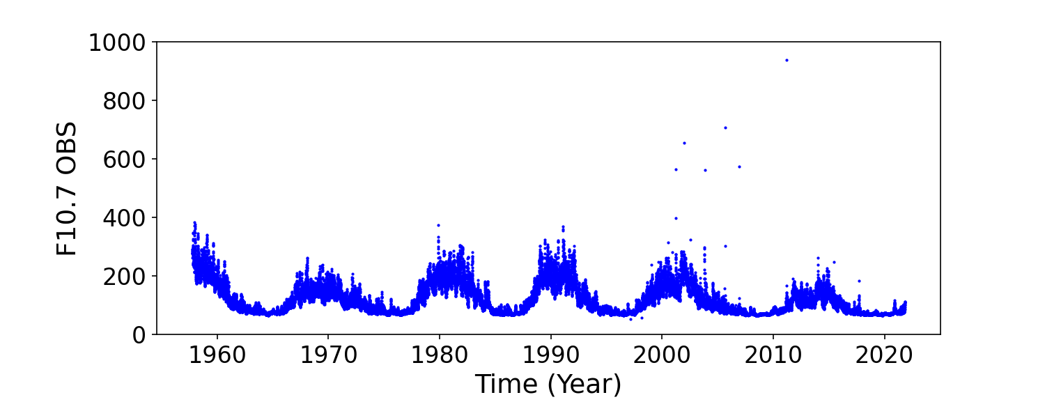
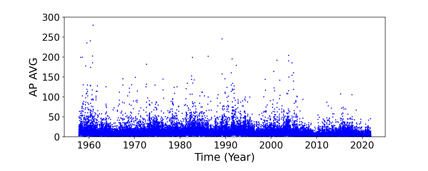
Figure 1: Space weather data vs. timestep from the EOP and Space Weather Data

As a first step for a more complete study, we used Naive one-step time-series forecasting to predict the value of the parameters already mentioned, F10.7 OBS and AP AVG. The last 365 time steps (one year) are used as a test set to evaluate a very simple naively forecasting method, fitted on all the remaining observations. This strategy of forecasting simply teaks the previous period and applies it to the actual one. The walk-forward validation method is used to measure the performance of the model, where we applied one separate one-step forecast to each of the test observations. The true data was then added to the training set for the next forecast. We used the Mean absolute percentage error regression loss (MAPE) to compare our results with the real test set. This metric is defined in