Abstract

After the successful full-shape analyses of BOSS data using the Effective Field Theory of Large-Scale Structure, we investigate what upcoming galaxy surveys might achieve. We introduce a “perturbativity prior” that ensures that loop terms are as large as theoretically expected, which is effective in the case of a large number of EFT parameters. After validating our technique by comparison with already-performed analyses of BOSS data, we provide Fisher forecasts using the one-loop prediction for power spectrum and bispectrum for two benchmark surveys: DESI and MegaMapper. We find overall great improvements on the cosmological parameters. In particular, we find that MegaMapper (DESI) should obtain at least a 12$\sigma$ ($2\sigma$) evidence for non-vanishing neutrino masses, bound the curvature $\Omega_{k}$ to 0.0012 (0.012), and primordial inflationary non-Gaussianities as follows: $f_{\text{NL}}^{\text{loc.}}$ to $\pm 0.26$ (3.3), $f_{\text{NL}}^{\text{eq.}}$ to $\pm 16$ (92), $f_{\text{NL}}^{\text{orth.}}$ to $\pm 4.2$ (27). Such measurements would provide much insight on the theory of Inflation. We investigate the limiting factor of shot noise and ignorance of the EFT parameters.

1 Introduction and Summary

In the last few years, Large-Scale Structure (LSS) survey data have started to be analyzed using the so-called Effective Field Theory of Large-Scale Structure (EFTofLSS) [1, 2]. The approach in which the data are analyzed in the context of this theory is rather simple: all data below a certain maximum wavenumber are used in the Bayesian inference. This technique goes under the name of “full shape analysis”. Such an application to data has allowed a measurement of all cosmological parameters of the $\Lambda$CDM model using just a prior from Big Bang Nucleosynthesis [3, 4, 5]. The precision and accuracy achieved through this measurement were unexpectedly high, offering a new independent method for determining the Hubble constant with a percent-level precision [3], and for measuring $\Omega_{m}$ with a precision comparable to Planck [6], among other remarkable achievements. For the interested reader we provide a list of references of the application of the EFTofLSS to data in this footnote . It should be stressed that the development of the EFTofLSS was a rather long journey in which the theory was developed in the various stages that are necessary to compare it to observations (dark matter, galaxies, redshift space distortions, IR-resummation, fast-evaluation techniques, MonteCarlo sampling, etc.), and along the way comparison with numerical simulations was essential to check that the theory was on the right track. Because of this, we find it fair, and also useful for the interested reader, to provide a footnote with a list of the references that were essential for the development of the EFTofLSS prior to its application to data, when it finally became clear that the approach was useful .

So far, the data analysis has mainly focused on the data from BOSS DR12 [87]. While there are certainly more ways in which these data can be analyzed, with many much-improved LSS surveys coming online and being designed, it is natural to ask what kind of measurement the application of the so-far developed EFTofLSS to these data will allow. In this paper, we do this by Fisher forecasting the information content of two upcoming surveys, that we take as benchmarks, DESI [88], and MegaMapper [89], including some forecasts for further analyses on BOSS. Our intention is that the results for these two upcoming and planned surveys will give an idea of the capabilities of other further surveys, either already planned or to be planned. We primarily focus on the cosmological parameters of the flat $\Lambda$CDM model, while also considering neutrino masses, curvature, and primordial non-Gaussianities (for a forecast about CDM-isocurvature modes for Euclid and MegaMapper, using just the one-loop power spectrum and tree level bispectrum, see [90]). These are in fact parameters whose detection would allow us to extend or ameliorate the standard model of cosmology and of particle physics.

For neutrinos, we know from neutrino oscillations that they are massive (see for example [91]), but we do not know the absolute value of their masses. For inflation, curvature should naturally be very small, to the order of the primordial perturbations $\sim 3\cdot 10^{-5}$, though evidence of negative curvature could be extremely interesting, pointing towards the fact that our universe might come out of a bubble nucleation event (see for example [92] and references therein). A large positive curvature would essentially rule out eternal inflation, while a large negative curvature would rule out slow-roll eternal inflation [93]. Finally, non-Gaussianities could reveal the interaction structure of Inflation, which is actually the most insightful aspect to understand the particle physics origin of this theory. Concerning the shape of the non-Gaussianities we will explore, we will analyze the so-called $f_{\text{NL}}^{\text{loc.}}$ (see e.g. [94]), $f_{\text{NL}}^{\text{eq.}}$ [95] and $f_{\text{NL}}^{\text{orth.}}$ [96] shapes, which parametrize a large class of non-Gaussianities that can be produced in single field inflation [97, 96], and, for $f_{\text{NL}}^{\text{loc.}}$, also in multifield inflation (see e.g. [98, 99, 100, 101]) (see also recently [102] for a forecast on MegaMapper on these parameters using just the tree-level bispectrum). It should be stressed that there exist other shapes of non-Gaussianities that are well motivated (see e.g. [103]), and we leave their exploration to future work.

Let us summarize some important technical aspects of our analysis:

• We use the prediction of the EFTofLSS at one loop order for the power spectrum and the bispectrum. We provide the Fisher forecasts by utilizing all the multipoles of the line-of-sight angle.

• The model that we implement is the same as in the analyses of the BOSS data as in [14]. In particular, this includes the integration of the one-loop bispectrum integrals as developed in [104]. The modeling of primordial non-Gaussianities is done as in [28].

• We check the accuracy of our predictions against comparison with the posterior obtained by analyzing the BOSS data with the full-likelihood of [14]. We conclude that, approximately, our predictions for the error bars should be roughly accurate to about $30\%$ or $40\%$, once the maximum wavenumber of the analysis has been fixed. This error is primarily influenced by our assumption of a diagonal covariance.

On top of the overall volume of the survey, we identify two limiting factors that affect the precision of the upcoming measurements. One is the discreteness of the galaxy field, which induces a shot noise term in the data, and the second is the fact that dozens of EFT parameters, including biases, need to be fitted to the observations (these EFT parameters encode the effect at long distances from uncontrolled short distance physics, which includes the relation between galaxy overdensities and matter fields). We explore these issues in the following way:

1. Shot noise: In addition to our main analysis, we provide Fisher forecasts with shot noise set to zero, effectively assuming an infinitely dense distribution of galaxies.

2. EFT parameters: We investigate the impact of limited knowledge regarding the EFT parameters by conducting Fisher forecasts in the following three ways:

   1. We set the width of the prior on the EFT parameters to zero, which is equivalent to fixing them. This represents the ultimate reach in terms of constraining power.

   2. Galaxy Formation Prior: We set the width of the prior on the EFT parameters to 0.3 (rather than about $2$ or 4 as in the normal analyses). This is meant to represent a perhaps realistic prior on the EFT parameters as informed by astrophysical galaxy formation studies.

   3. Perturbativity Prior: Finally, we introduce a new, theoretically-justified prior on the EFT parameters that we call “perturbativity prior”, which is based on the following reasoning. In the EFTofLSS, it is possible to estimate the correct size of a loop term given the lower order terms by simple scaling formulas. It is self-consistent to impose that the loop terms in the analysis obey this estimate. If the number of parameters to fit to observations is small, this criterium is automatically satisfied once the EFT parameters have been assigned a prior of ${\cal{O}}(1)$, which is the standard way in which priors are set (see for e.g. [14]). However, when the number of parameters becomes large, say $n\gg 1$, if each parameter is ${\cal{O}}(1)$, the size of the loop can be a factor of ${\cal{O}}\left(\sqrt{n}\right)$ too large, due to some random accumulation effect. It is easy to convince oneself that the data, which are most effective at the highest wavenumbers where the loop is sizable, might not provide sufficient constraining power to prevent such random accumulation effects from happening. In fact, due to cancellations among the various components of a loop term, it is possible that the loop is small at those high wavenumbers where both data and loop are strong, while the loop could still be too large at intermediate and low wavenumbers. Indeed, at these intermediate and low wavenumbers, the data, being weaker, do not constrain the loop term, having this one become quite smaller in the meantime. We therefore set a Gaussian prior on the overall loop term, by favoring the configurations that satisfy the overall size and scaling as a function of wavenumber of the loop term. While this prior has not yet been tested on simulations or data, it is solidly theoretically justified, and we report results incorporating it.

We find the following results for DESI and MegaMapper for the various cosmological parameters:

• $\Omega_{k}$: Planck 2018 constrains this parameter to 0.0065 [6]. For DESI, we forecast a constraint of about 0.051. MegaMapper instead will reduce this bound to 0.0012, representing an improvement of over 5 times compared to Planck, and just about 1.5 orders of magnitude away from the ultimate limit where it makes sense to measure this parameter, which is the amplitude of the primordial curvature fluctuation. We notice however that this bound depends quite strongly on the maximum wavenumber of the analysis.

• $\sum_{i}m_{\nu_{i}}$: Planck 2018 constrains this parameter to be $<$0.27 eV [6]. However, the most interesting side of the error for this parameter is the lower one, as it is associated to a detection of non vanishing masses. We find that DESI will constraint this parameter to about $-0.07$ eV from above the reference value (which is what is relevant for detection) with only the power spectrum (P) and $-0.05$ eV with the addition of the bispectrum, a significant improvement with respect to Planck. Since our bound depends on the central value of neutrino masses, a more invariant way to cast this bound is that we expect on DESI there will be a guaranteed $2\sigma$-evidence for non vanishing neutrino masses. MegaMapper instead will reduce this bound to 0.008 eV, which should guarantee a $\gtrsim 12\sigma$ detection. After the measurement of the cosmological constant $\Lambda$, this would be the second parameter of the standard model of particle physics that is measured from cosmological observations.

• $f_{\text{NL}}$: Planck 2018 constraints $f_{\text{NL}}^{\text{loc.}}$ to $\pm 5$, $f_{\text{NL}}^{\text{eq.}}$ to $\pm 47$, $f_{\text{NL}}^{\text{orth.}}$ to $\pm 24$ [105]. We find that DESI will constraint $f_{\text{NL}}^{\text{loc.}}$ to $\pm 3.3$, $f_{\text{NL}}^{\text{eq.}}$ to $\pm 92$ (or $\pm 114$ without the perturbativity prior), $f_{\text{NL}}^{\text{orth.}}$ to $\pm 27$, which are quite comparable to the limits obtained by Planck. MagaMapper will further reduce these bounds as $f_{\text{NL}}^{\text{loc.}}$ to $\pm 0.26$, $f_{\text{NL}}^{\text{eq.}}$ to $\pm 16$ (or $\pm 18$ without the perturbativity prior), $f_{\text{NL}}^{\text{orth.}}$ to $\pm 4$. These are very significant improvements with respect to Planck, that range from factors of almost three for $f_{\text{NL}}^{\text{eq.}}$, six for $f_{\text{NL}}^{\text{orth.}}$, to about a factor of 20 for $f_{\text{NL}}^{\text{loc.}}$. Such a level of improvement brings with it a clear chance of a discovery of primordial non-Gaussianities, opening the door to a deeper understanding at the particle physics level of the inflationary theory. Additionally, the allowed values for non-Gaussianities would begin to be close to that ${\cal{O}}(1)$ which represents the vague but significant threshold beyond which inflation is of the slow-roll kind.

We also study the limiting effect of shot noise and biases. We find that setting the shot noise to zero for DESI would reduce the error bars of practically all parameters by roughly a factor of two. For MegaMapper, the reduction would be of a factor of about three for the $f_{\text{NL}}$’s, and about an order of magnitude for the other cosmological parameters.

Regarding the EFT parameters, assuming perfect prior knowledge of the biases in DESI would lead to varied reductions in the error bars, typically by a factor of two. For $f_{\text{NL}}^{\text{eq.}}$, the reduction would be around a factor of five. When considering our galaxy-formation benchmark prior of 0.3 instead of fixed parameters, the improvement is significantly diminished to approximately 30% for $f_{\text{NL}}^{\text{eq.}}$ and $f_{\text{NL}}^{\text{orth.}}$, with marginal impact on the other parameters. We find a similar behavior for MegaMapper. It appears that the perturbativity prior only captures a fraction of the potential improvement achievable through exact knowledge of the biases. It would be interesting to see if higher $n$-point functions or higher-order computations can improve on this.

Overall, this Fisher analysis tells us that even by just using the EFTofLSS at the current level of development, the next decade in LSS surveys could lead to great improvements in our knowledge of cosmological parameters. This includes parameters that have not yet been measured, such as neutrino masses, as well as those connected to inflation, such as primordial non-Gaussianities and the curvature of the universe. Improvements in the design of surveys to reduce shot noise, or advancements in the measurement of EFT parameters have the potential to further strengthen these already promising results.

Public Codes:

The code to compute the Fisher forecasts is publicly available on GitHub .

2 Technical aspects of the Fisher Matrix

Fisher analyses have become a key tool for forecasting in cosmology. Pioneered in [106], there have been numerous applications over the past years (for example [107, 108, 109]). We here briefly lay out which methods we will use for our forecasts and what contributes to our estimates.

At the heart of Fisher forecasts lies the Cramér-Rao lower bound. It states that the covariance of unbiased estimators for a set of parameters $\theta$ is bounded below by the inverse of the Fisher information matrix $F_{ij}$, defined as the expected value of the Hessian of the log-likelihood

$$F_{ij}=-\bigg{\langle}\frac{\partial^{2}\log L}{\partial\theta_{i}\partial\theta_{j}}\bigg{\rangle}.$$ (2.1)

Under the assumption that the likelihood is Gaussian with mean $X$ and covariance $C$, we can approximately write the Fisher matrix as [106]

$$F_{ij}=\frac{\partial X^{T}}{\partial\theta_{i}}C^{-1}\frac{\partial X}{\partial\theta_{j}}.$$ (2.2)

In order to calculate the Fisher matrix, we need to assume reference parameters $\theta^{\text{ref}}$, on which we evaluate the derivatives. In particular, the reliability of the Fisher forecast depends on this reference cosmology being fairly accurate. An intuitive way to see the reference cosmology dependence and also an alternative derivation for Eq. (2.2) is to start directly with a Gaussian likelihood for an observable $X$ depending on parameters $\theta$, that has a true mean $\tilde{X}$, such that the log-likelihood is given by

$$-2\log L=(X(\theta)-\tilde{X})^{T}C^{-1}(X(\theta)-\tilde{X})+p_{1},$$ (2.3)

where $p_{1}$ is a $\theta$-independent constant. We can then assume a reference value $\theta^{\text{ref}}$, and Taylor expand around the reference value to first order, $X(\theta)\simeq X(\theta^{\text{ref}})+\sum_{i}\frac{\partial X}{\partial\theta_{i}}(\theta_{i}-\theta_{i}^{\text{ref}})$. If $X(\theta^{\text{ref}})$ is accurate we can identify that the $\tilde{X}$ term in Eq. (2.3) cancels with $X(\theta^{\text{ref}})$ (). What remains is the first order term, which we can substitute back into Eq. (2.3), to get

$$-2\log L=(\theta-\theta^{\text{ref}})^{T}F(\theta-\theta^{\text{ref}})+p_{1},$$ (2.4)

where we get the same formula for the Fisher matrix, $F$, as in Eq. (2.2). In Eq. (2.4) we can now clearly see that the Fisher matrix is the inverse covariance for the likelihood of the parameter vector $\theta$. As can be seen from the derivation above, the Fisher formalism is sensitive to an accurate reference cosmology in order for $\tilde{X}$ to cancel with $X(\theta^{\text{ref}})$ and also for the Taylor expansion to be an accurate approximation. Given that we now have precise measurements of all cosmological and EFT parameters [110] we have good reason to believe we are making realistic predictions around a realistic reference cosmology. In fact, we will show in Sec. 3 that we can reproduce results from previous surveys to great precision. We also checked that slight deviations from this reference cosmology do not greatly alter our results.

Note that Eq. (2.2) is in principle simply an inverse-covariance weighted sum over all available information. Both the mean and the covariance can be modeled using perturbation theory. We will discuss this in Secs. 2.1 and 2.2. Then in Sec. 2.3 we will discuss further ingredients that go into calculating the Fisher matrix, such as fixing the reference bias parameters at different redshifts. We here always refer to the correlators of galaxies in redshift space. Therefore, unless explicitly mentioned, we drop the ^h,r index with respect to the notation in [111], and by $P,B,\delta,...$ we always indicate the quantities for biased tracers in redshift space.

2.1 Power spectrum and bispectrum

For both the power spectrum and bispectrum there are well-established thin-shell averaged estimators that predict the mean and covariance for Eq. (2.2). We use the estimators that bin in the momenta, but not in the line of sight , since we have enough analytical control to integrate over the full line of sight information.

Furthermore, for both correlators, we use leading-order contributions in the covariance, in particular neglecting power spectrum-bispectrum cross-covariance. We will discuss the impact of this approximation in Sec. 3.2. This assumption in particular implies that we can write the combined power spectrum and bispectrum Fisher matrix, $F^{P+B}$, as the sum of the individual Fisher matrices

$$F^{P+B}=F^{P}+F^{B},$$ (2.5)

where $F^{P}$ and $F^{B}$ are the power spectrum and bispectrum Fisher matrices respectively. Next, we will discuss these individual contributions.

Power spectrum

For the power spectrum, the estimator is given by [106, 112]

$$\hat{P}(k;\hat{z})=\frac{1}{V_{S}V_{P}(k)}\int_{\Delta B_{k}}d^{3}q\delta(q;\hat{z})\delta(-q;\hat{z}),$$ (2.6)

where we used the notation $\Delta B_{k}=B(0,k+\frac{\Delta k}{2})\backslash B(0,k-\frac{\Delta k}{2})$ and $B(a,r)$ is the ball of radius $r$ around the point $a$. $V_{S}$ is the survey volume and $V_{P}(k)=4\pi k^{2}\Delta k$ is a normalization factor given by just the integral on the right-hand side of Eq. (2.6) without the prefactors and with the galaxy density contrast $\delta\rightarrow 1$, i.e. $V_{P}(k)=\int_{\Delta B_{k}}d^{3}q$.

The expected value of the estimator is simply the power spectrum itself and we will evaluate it up to the one-loop order. That is

$$P=P_{\text{Tree}}+P_{1L}.$$ (2.7)

Here the tree and loop contributions include their respective stochastic and response terms. We use the exact same model as in [110, 111]. Then, for the covariance, we get

$$C_{PP}(k,k^{\prime}) = \langle\hat{P}(k)\hat{P}(k^{\prime})\rangle-\langle\hat{P}(k)\rangle\langle\hat{P}(k^{\prime})\rangle$$

$$= \frac{1}{V_{S}^{2}V_{P}^{2}(k)}\int_{\Delta B_{k}\times\Delta B_{k}^{\prime}}d^{3}q_{1}d^{3}q_{2}\bigg{[}\langle\delta(q_{1};\hat{z})\delta(-q_{1};\hat{z})\delta(q_{2};\hat{z})\delta(-q_{2};\hat{z})\rangle$$

$$\qquad-\langle\delta(q_{1};\hat{z})\delta(-q_{1};\hat{z})\rangle\langle\delta(q_{2};\hat{z})\delta(-q_{2};\hat{z})\rangle\bigg{]}$$

$$= \frac{2}{V_{S}^{2}V_{P}^{2}(k)}\int_{\Delta B_{k}\times\Delta B_{k}^{\prime}}d^{3}q_{1}d^{3}q_{2}\langle\delta(q_{1};\hat{z})\delta(q_{2};\hat{z})\rangle\langle\delta(-q_{1};\hat{z})\delta(-q_{2};\hat{z})\rangle$$

$$= \delta_{k,k^{\prime}}\frac{4\pi^{2}}{V_{S}k^{2}\Delta k}P_{\text{Tree}}(k;\hat{z})^{2}.$$

Note that, schematically, we used $\langle\delta\delta\delta\delta\rangle=\langle\delta\delta\delta\delta\rangle_{c}+3\langle\delta\delta\rangle\langle\delta\delta\rangle$, where, by the subindex _c, we mean the connected correlator. The connected four-point function is the trispectrum, which we neglect here. Of the three disconnected parts one cancels with the $\langle\hat{P}(k)\rangle\langle\hat{P}(k^{\prime})\rangle$ term in the first line and the other two terms are the same, giving the factor of two in the third line. As mentioned, off-diagonal contributions to the above covariance are of the order of the trispectrum, and therefore similar in size to the one-loop power spectrum multiplied by a linear power spectrum. To be consistent in the perturbative order, given that we neglect the off-diagonal contributions, we also neglect loop contributions to the diagonal of the covariance. We will see in Sec. 3 that this leads to a roughly $10\%$ effect. Finally, by substituting the mean and covariance into Eq. (2.2) we get the power spectrum Fisher matrix

$$F_{ij}^{P}=\sum_{k}\frac{k^{2}V_{S}}{4\pi^{2}\Delta k}\int_{-1}^{1}\frac{d\mu}{2}\frac{\partial P(k;\hat{z})}{\partial\theta_{i}}\frac{\partial P(k;\hat{z})}{\partial\theta_{j}}\frac{1}{\left(P_{\text{Tree}}(k;\hat{z})\right)^{2}},$$ (2.9)

with $\mu=\hat{k}\cdot\hat{z}$ the line of sight angle.

Bispectrum

For the bispectrum, we use the estimator [113, 114]

$$\hat{B}(k_{1},k_{2},k_{3};\hat{z})=\frac{1}{V_{S}V_{B}(k_{1},k_{2},k_{3})}\int\limits_{\Delta B_{k_{123}}}d^{3}q_{1}d^{3}q_{2}d^{3}q_{3}\delta_{D}(q_{1}+q_{2}+q_{3})\delta(q_{1};\hat{z})\delta(q_{2};\hat{z})\delta(q_{3};\hat{z}),$$ (2.10)

where we defined $\Delta B_{k_{123}}=\Delta B_{k_{1}}\times\Delta B_{k_{2}}\times\Delta B_{k_{3}}$. Similarly to the power spectrum discussion, the volume $V_{B}$ is defined by just the above integral with $\delta\rightarrow 1$ , without prefactors and is given by

$$V_{B}(k_{1},k_{2},k_{3}) = \int\limits_{\Delta B_{k_{123}}}d^{3}q_{1}d^{3}q_{2}d^{3}q_{3}\delta_{D}(q_{1}+q_{2}+q_{3})$$

$$= 8\pi^{2}k_{1}k_{2}k_{3}\Delta k_{1}\Delta k_{2}\Delta k_{3}\beta(k_{1},k_{2},k_{3}),$$

where, without loss of generality, we assume $k_{3}\geq k_{2}\geq k_{1}$ and $\beta(k_{1},k_{2},k_{3})=1$ unless $k_{3}=k_{1}+k_{2}$, in which case it is $\frac{1}{2}$. Again the mean of this estimator is simply the bispectrum itself, which we calculate up to the one-loop order as in [111]:

$$B=B_{\text{Tree}}+B_{1L}.$$ (2.12)

Again the tree and loop contributions include their respective stochastic and response terms. To leading order, the bispectrum-bispectrum covariance is given by 

$$C_{BB}(k_{1},k_{2},k_{3},k_{1}^{\prime},k_{2}^{\prime},k_{3}^{\prime}) = \frac{(2\pi)^{6}}{V_{S}V_{B}(k_{1},k_{2},k_{3})}s_{B}\prod_{i=1}^{3}\left(\delta_{k_{i},k_{i}^{\prime}}P(k_{i};\hat{z})\right),$$ (2.13)

where $s_{B}$ is a symmetry factor that is equal to 6 for equilateral triangles, 2 for isosceles triangles and 1 otherwise. Again, we do not consider off-diagonal contributions, which would be the connected six-point function, as well as bispectra squared and products of trispectra and power spectra. While these contributions are suppressed relative to the diagonal, they may be sizable in some cases and we therefore check this approximation with respect to covariances measured in mocks in Sec. 3. Finally, we bin equally in all $k_{i}$, so that if we plug Eq. (2.12) and Eq. (2.13) in to Eq. (2.2), we get the bispectrum Fisher matrix at fixed redshift (see Sec. 4.2 of [107] or Sec. 4.1.3 of [116] for more details):

$$F_{ij}^{B}=\frac{V_{S}}{(2\pi)^{5}}\sum_{(k_{1},k_{2},k_{3})}\frac{1}{s_{B}}\int_{-1}^{1}\int_{0}^{2\pi}d\mu_{1}d\phi\frac{\partial B}{\partial\theta^{i}}\frac{\partial B}{\partial\theta^{j}}\prod_{i=1}^{3}\left(\frac{k_{i}\Delta k}{P_{\text{Tree}}(k_{i};\hat{z})}\right)\begin{cases}\frac{1}{2},\text{if }k_{3}=k_{1}+k_{2}\\ 1,\text{else}\\ \end{cases},$$ (2.14)

where $\mu_{i}(\mu_{1},\phi)=\hat{k_{i}}\cdot\hat{z}$ are the projected momenta, and we omitted writing the arguments of $B$ to avoid clutter. We use the same parametrization of the $\mu_{i}$ as for example in [110, 111].

2.2 Combining redshifts

In the previous section, we derived formulas for Fisher matrices for the power spectrum and bispectrum at a single redshift. However, for surveys that cover a range of redshifts, we need to combine the information from different redshift bins to compute the overall Fisher matrix. We will now lay out how we combine these redshifts.

Assuming that all EFT-parameters at different redshifts are uncorrelated , the full Fisher matrix for a survey with a set of redshift bins can be expressed as the sum of the power spectrum Fisher matrix and the bispectrum Fisher matrix over the redshift bins

$$F_{\text{survey}}=\sum_{z}{\left(F^{P}(z)+F^{B}(z)\right)}.$$ (2.15)

In all forecasts we consider, we split the survey into two sets of redshift bins, let us call them $\text{bin}_{1}$ and $\text{bin}_{2}$. Let us write $F_{\text{survey}}=F_{\text{survey},1}+F_{\text{survey},2}$ and the sum in Eq. (2.15) for each of these two Fisher matrices simply runs over the redshifts in that particular set of bins (for BOSS this is, for example, LOWZ and CMASS, i.e. $\text{bin}_{1}=\{z\in$ Tab. 5 $|z\leq 0.45\}$ and $\text{bin}_{2}=\{z\in$ Tab. 5 $|z>0.45\}$). A common approach is then to define effective redshifts $z_{\text{eff}}$, background number density $n_{b,\text{eff}}$, etc., and simply compute the $F_{\text{survey},i}$ with these values. This is a good approximation for the derivatives of the observables, given that the time dependence is largely dominated by the growth factors that have comparably weak time dependence. However, we find that this is not a very accurate estimate for the covariance . To emphasize the different redshift-dependent contributions that enter the covariance, let us write the covariance from the previous sections in their full form:

$$C_{PP}(k,k^{\prime};z) = \delta_{k,k^{\prime}}\frac{4\pi^{2}}{V_{S}(z)k^{2}\Delta k}\left((b_{1}(z)+f(z)\mu^{2})^{2}P_{11}(k)+\frac{c_{1}^{St}}{n_{b}(z)}\right)^{2}$$ (2.16)

$$C_{BB}(k_{i},k_{i}^{\prime};z) = \frac{32\pi^{4}s_{B}\prod_{i=1}^{3}\left(\delta_{k_{i},k_{i}^{\prime}}\right)}{V_{S}(z)k_{1}k_{2}k_{3}\Delta k^{3}\beta(k_{1},k_{2},k_{3})}\prod_{i=1}^{3}\left((b_{1}(z)+f(z)\mu_{i}^{2})^{2}P_{11}(k_{i})+\frac{c_{1}^{St}}{n_{b}(z)}\right),$$

where $P_{11}$ is the linear dark matter power spectrum, $c_{1}^{St}$ is the tree-level stochastic term and we abbreviated the triangle dependence on the left-hand side $k_{i}=\{k_{1},k_{2},k_{3}\}$. Defining effective numbers as an approximation is not appropriate for the covariance since it is very sensitive to accurate estimates of the survey volume $V_{S}$, number density $n_{b}$, and linear bias $b_{1}$. Their numerical values are typically given by survey specifications, and vary greatly with redshift. Specifically, $n_{b}$ greatly varies with redshift as it depends on the survey target selection and measurements. In contrast, the growth rate $f$ and the linear power spectrum $P_{11}$ have a comparably mild redshift dependence. However, in our analysis, we will nevertheless consider their redshift dependence for completeness.

To summarize, we have weak time dependence in the derivatives and strong redshift dependence in the covariance. Therefore, for $X\in\{P,B\}$ and $i\in\{1,2\}$ we use the following approximation for the Fisher matrix of the two redshift bins: 

$$(F_{\text{survey},r}^{X})_{ij} = \sum_{z\in\text{bin}_{r}}\frac{\partial X^{T}(z)}{\partial\theta_{i}}C_{XX}^{-1}(z)\frac{\partial X(z)}{\partial\theta_{j}}$$

$$\simeq \frac{\partial X^{T}(z_{\text{eff},r})}{\partial\theta_{i}}\left(\sum_{z\in\text{bin}_{r}}C_{XX}^{-1}(z)\right)\frac{\partial X(z_{\text{eff},r})}{\partial\theta_{j}},$$

where $z_{\text{eff},r}$ is the effective redshift for $\text{bin}_{r}$. The vector contractions in Eq. (2.2), represent the covariance weighted sum over the available information in the correlator $X$. For the modes, this leads to the sums over $k$ in Eq. (2.9) and Eq. (2.14). We also sum over all redshift space information, which in the continuum limit turns into an integral over the redshift space angles in Eq. (2.9) and Eq. (2.14). The final full Fisher matrix that we use is $F_{\text{survey}}=F^{P}_{\text{survey},1}+F^{B}_{\text{survey},1}+F^{P}_{\text{survey},2}+F^{B}_{\text{survey},2}$.

2.3 Survey specifications at different redshifts

Now that we established how to combine the information from different redshifts, let us discuss what reference parameters we choose for each of these redshifts. Predictions from the EFTofLSS rely on a number of redshift and survey-dependent parameters. While these factors have been measured to great precision at low redshifts for the BOSS survey, we need to discuss how we extrapolate these results to different redshifts and surveys.

EFT parameters

Let us first look at the approximate evolution of all EFT parameters entering the galaxy power spectrum and bispectrum. In particular, we analyze the time dependence of the physical (as opposed to the bare) parameters. There are at least two distinct origins of nuisance parameters in the EFTofLSS. On the one hand, we expand some functions (such as the stress tensor or the galaxy overdensity) in terms of all fields they can depend on, multiplied by parameters. Schematically at linear order, with redshift space distortions implied, this is (see for example [111])

$$\delta(x,t)=b_{1}(t)\delta_{\text{dm}}(x,t)+...-c_{1}^{h}(t)\frac{k^{2}}{k_{\text{NL}}^{2}}\delta_{\text{dm}}(x,t)+...\;,$$ (2.18)

where $\delta_{\text{dm}}$ is the dark matter overdensity (note that $\delta$ without indices always denotes the overdensity of galaxies in redshift space). We will refer to these parameters as biases (this includes response terms, but not stochastic fields). The BOSS best-fit for the biases, $\vec{b}_{\text{BOSS}}$, has been determined in [110]. The explicit numerical values are in App. A. When fixing the reference cosmology for surveys at higher redshifts, we rescale the biases according to the estimated linear bias given in the survey specifications [88, 117]. Specifically for any new survey we set the reference value for the vector of biases $\vec{b}=\{b_{1},b_{2},...,c_{1}^{h},c_{2}^{h},...\}$ according to

$$\vec{b}^{\text{ref}}=\frac{b_{1}^{\text{ref}}}{b_{1,\text{BOSS}}}\vec{b}_{\text{BOSS}}.$$ (2.19)

Note that the $b_{1}^{\text{ref}}$ in the tables of Sec. 4, App. A and [88, 117], account for different redshifts and different galaxy species. For the surveys we consider in this paper, we give the numerical values for $b_{1}^{\text{ref}}$ in Tabs. 1, 2 and 3.

Contrary to biases, there are parameters coming from correlators of stochastic fields. For example, we have

$$\langle\delta(k,t)\delta(k^{\prime},t)\rangle^{\prime}\supset\langle\epsilon_{A}(k,t)\epsilon_{B}(k^{\prime},t)\rangle^{\prime}=\frac{1}{n_{b}}\left(c_{1}^{St}+c_{2}^{St}\frac{k^{2}}{k_{\text{NL}}^{2}}+...\right).$$ (2.20)

We will call these terms stochastic. Importantly, since they are Poisson distributed, they are constant in time. Therefore, given that we have a vector of measured values for the stochastic terms from BOSS, we could in principle use these reference values for all redshifts. However, we here make a slight correction relative to the analysis done in [110]. There, leading order stochastic terms, for example $c_{1}^{St}$, were varied freely, whereas they should be fixed to one, by definition of ${n_{b}}$ (). Therefore, for surveys other than BOSS, we fix the leading order stochastic parameters for the power spectrum and bispectrum, i.e. $c_{1}^{St,\text{ref}}=c_{1}^{(222),\text{ref}}=1$, and we also do not take derivatives with respect to these parameters . For all other terms in the vector of stochastic terms $\vec{\epsilon}=\{c_{2}^{St},c_{3}^{St},...\}$ we use

$$\vec{\epsilon}^{\ \text{ref}}=\frac{1}{c^{St}_{1,\text{BOSS}}}\vec{\epsilon}_{\text{BOSS}},$$ (2.21)

where $\vec{\epsilon}_{\text{BOSS}}$ is the vector of stochastic parameters measured for BOSS . Explicit numerical values are given in App. A and for details on the specific parameters see [111].

As a final remark, we note that we have tested the sensitivity of our results in Sec. 4 to small shifts in the reference values of EFT parameters and found that they do not significantly affect our findings. The parameters that have the greatest impact on our results are those used in the modeling of the covariance, namely $b_{1}$ and $c_{1}^{St}$. To ensure accurate predictions for future surveys, where the best-fit is yet unknown, we take $b_{1}^{\text{ref}}$ directly from survey specifications and we set the reference value of $c_{1}^{St}$ to one (with the exception of BOSS, as mentioned earlier).

Perturbative reach

The perturbative reach of the EFTofLSS, parametrized by $k_{\text{max}}$, can be determined in simulations by setting a threshold for the theory systematic error. This was the approach used for example, in [110, 3, 19]. For the BOSS CMASS sample this is $k_{\text{max}}=0.22h\,{\rm Mpc}^{-1}$ at one-loop order and $k_{\text{max}}=0.1h\,{\rm Mpc}^{-1}$ at tree level. In the following, we will lay out how we estimate the $k_{\text{max}}$ for a different survey at a different redshift, motivated by the method used in [3]. There, roughly, it was imposed that the signal-to-noise of the leading theoretical error should not be sizable in the $k$-bin containing the $k_{\text{max}}$ (see footnote 23 in [3]). This is a good approximation, assuming that the signal-to-noise of the theoretical error only has a sizeable contribution in the highest $k$-bin. Here, however, we want to limit the full signal-to-noise of the theoretical error over all $k$-bins. The motivation for this is two-fold. First, this approach is binning independent, which is important to be consistent between surveys that have different bin sizes. Second even though the signal-to-noise of the leading theoretical error is well approximated by only considering contributions at large $k$ since it grows very steeply with $k$, it leads to a slight overestimate of the $k_{\text{max}}$ () since one does not consider the theoretical error at $k<k_{\text{max}}-\frac{\Delta k}{2}$. We, therefore, consider the theoretical error contribution at all scales. Furthermore, as was used in [110], we will use the same $k_{\text{max}}$ for the power spectrum and the bispectrum, since we expect the $k$-reach to be the same. To summarize, this means we impose that the signal-to-noise of the theoretical error is the same in all surveys, which then defines the $k_{\text{max}}$ through

$$\sum_{k=k_{\text{min}}}^{k_{\text{max,1}}}\left(\frac{\sigma_{\text{theory,1}}(k,z_{1},...)}{\sigma_{\text{data,1}}(k,z_{1},...)}\right)^{2}=\sum_{k=k_{\text{min}}}^{k_{\text{max,2}}}\left(\frac{\sigma_{\text{theory,2}}(k,z_{2},...)}{\sigma_{\text{data,2}}(k,z_{2},...)}\right)^{2},$$ (2.22)

where the sum runs over the $k$-bins of the respective survey, the dots represent further dependences, such as the EFT-parameter best-fit, and $\sigma_{\text{data/theory,i}}$ are the respective theoretical and data errors that we will discuss next. The leading theoretical error is the next higher loop contribution, and we estimate the data error by perturbatively modeling the covariance. Let us focus on the theoretical error first. To good approximation [40] the $L$-th order loop scaling is given by

$$\sigma_{L-\text{Loop}}(k,z)=P_{11}(k,z)\left(\frac{k}{k_{\text{NL}}(z)}\right)^{(3+n(k,z))L},$$ (2.23)

where $n(k,z)$ is the slope of the linear power spectrum around $k$. For the one-loop analysis, the theoretical error is, therefore, $\sigma_{\text{theory,i}}(k,z_{i},...)=\sigma_{2-\text{Loop}}(k,z_{i})$. Note that in Eq. (2.22), any constant factor will drop out, so we only care about the scaling. Furthermore given that from the BOSS analysis we have $k_{\text{NL}}^{\text{BOSS}}=0.7h\,{\rm Mpc}^{-1}$, we can get $k_{\text{NL}}$ at different redshifts by solving

$$\int_{0}^{{k_{\text{NL}}(z)}}dq\;q^{2}P_{11}(q,z)=\int_{0}^{0.7h\,{\rm Mpc}^{-1}}dq\;q^{2}P_{11}(q,z=0.57).$$ (2.24)

To estimate the data error we use the square root of the covariance estimate from Eq. (2.16), including the summation over redshifts, mentioned in Eq. (2.2). We average over the redshiftspace dependence, and do not consider shot noise , that is

$$\sigma_{\text{data},i}(k) = \left(\sum_{z\in\text{bin}_{i}}\int_{-1}^{1}\frac{d\mu}{2}C_{PP,n_{b}\rightarrow\infty}^{-1}(z,\mu)\right)^{-1/2}$$

$$= \frac{2\pi}{\sqrt{k^{2}\Delta k}}\left(\sum_{z\in\text{bin}_{i}}\frac{V_{S}(z)}{P_{11}(k,z)^{2}}\int_{-1}^{1}\frac{d\mu}{2}\frac{1}{\left(b_{1}(z)+f(z)\mu^{2}\right)^{4}}\right)^{-1/2}$$

$$=: \frac{\tilde{\sigma}_{\text{data},i}(k)}{\sqrt{\Delta k}}.$$

In practice, the sum over $z\in\text{bin}_{i}$ runs over the bins mentioned in Eq. (2.2). Furthermore, we defined $\tilde{\sigma}_{\text{data},\text{bin}_{i}}(k)$, since we will take the limit $\Delta k\rightarrow dk$, such that Eq. (2.22) turns into an integral with integration measure equal to $dk$. Then, for each survey bin with effective redshift $z_{\text{eff}}$, to estimate the $L$-th loop order $k_{\text{max}}^{L}$ , we solve

$$\int^{k_{\text{max}}^{L}}dk\frac{P_{11}(k,z_{\text{eff}})^{2}}{\tilde{\sigma}^{2}_{\text{data},i}(k)}\left(\frac{k}{k_{\text{NL}}(z_{\text{eff}})}\right)^{(3+n(k,z_{\text{eff}}))2(L+1)}$$ (2.26)

$$\qquad=\int^{k_{\text{max, CMASS}}^{L}}dk\frac{P_{11}(k,z=0.57)^{2}}{\tilde{\sigma}^{2}_{\text{data, CMASS}}(k)}\left(\frac{k}{0.7h\,{\rm Mpc}^{-1}}\right)^{(3+n(k,z=0.57))2(L+1)}\ .$$

2.4 Further ingredients from data analyses

In principle, we now have all the ingredients to compute Fisher forecasts for a given survey. However, there are a number of aspects related to the data and the data-analysis that we want to consider here, in order to best predict future results. For one, there are priors that we put on cosmological parameters and EFT parameters. For completeness we also briefly discuss the Alcock-Paczynski(AP) effect.

Priors

We impose priors on the EFT parameters that are very similar to those used in [110]. Given that we are assuming a Gaussian likelihood in the Fisher analysis, imposing a Gaussian prior amounts to adding the inverse variance of the prior to the diagonal of the Fisher matrix. The key difference between the priors we have in the Fisher analysis and those in the MCMC is that all of our priors are centered around the best-fit value rather than around zero. However, we have verified that this difference has a negligible impact on the error bars. For the special case of the linear bias $b_{1}$, we use a log-normal prior of variance 0.8 to ensure its positivity  For all other EFT parameters, we put a Gaussian prior of width 2, except for response and stochastic terms that are joint between the power spectrum and bispectrum, for which we use a Gaussian prior of width 4. These variance choices are analogous to the ones in [110].

We anticipate or hope that, in the coming years, our understanding of galaxy formation will advance to a level that will allow for stronger priors on the EFT parameters. In parts of Secs. 4 and 5.2 we, therefore, separately use a “galaxy-formation prior”, where we put a Gaussian prior of width $0.3$ on all EFT parameters, except for $b_{1}$ where we put again a log-normal prior, also with width $0.3$. This value of the prior is a benchmark value we deemed reasonably close to what can be potentially achieved.

For the cosmological parameters, we use a Gaussian Big-Bang Nucleosynthesis (BBN) prior on the baryon abundance $\omega_{b}$ centered around the best-fit value and, with a width of $\sigma_{\text{BBN}}=0.00036$. Also, we analyze $\log m_{\nu}^{\text{tot.}}:=\log(\sum_{i}m_{\nu_{i}}/\text{eV})$ rather than $\sum_{i}m_{\nu_{i}}$ which implicitly ensures unbounded positivity, with support $(0,\infty)$, on the neutrino masses, since the logarithm ensures positivity . In the results Sec. 4 we transform the predicted error on $\log m_{\nu}^{\text{tot.}}$ back to a $68\%$ interval on $\sum_{i}m_{\nu_{i}}$ (). We do not assume any previous knowledge about the other cosmological parameters. Overall, our choice of priors is almost equivalent to those used in the data analyses [110, 5].

Alcock-Paczynski effect

Galaxy spectra are measured on celestial coordinates. In order to transform to cartesian coordinates, a reference cosmology needs to be assumed, that might not correspond to the true cosmology. This discrepancy between the reference cosmology and the true cosmology introduces a geometric distortion known as the Alcock-Paczynski (AP) effect [119]. In order to account for this effect one has to evaluate the theory model on transformed wave numbers, given by

$$k=\frac{k^{\rm ref}}{q_{\perp}}\left[1+(\mu^{\rm ref})^{2}\left(\frac{1}{F^{2}}-1\right)\right]^{1/2}\,,\mu=\frac{\mu^{\rm ref}}{F}\left[1+(\mu^{\rm ref})^{2}\left(\frac{1}{F^{2}}-1\right)\right]^{-1/2}\,,$$ (2.27)

where

$$q_{\perp}=\frac{D_{A}(z)h}{D_{A}^{\rm ref}(z)h^{\rm ref}}\,,\qquad q_{\parallel}=\frac{H^{\rm ref}(z)/h^{\rm ref}}{H(z)/h}\,,\quad F=q_{\parallel}/q_{\perp},$$ (2.28)

and $D_{A}$ being the angular diameter distance.

Importantly, this transformation is invertible, and therefore, information preserving. Therefore, the AP effect does not lead to any addition or loss of information, when analyzing all (i.e. the full set of multipoles) information available from a given galaxy statistic at a given order. With the exception of a small part of Sec. 4.1, in Sec. 4 we will always analyze the full set of multipoles, where the AP effect is, therefore, irrelevant, and therefore we do not include it. The only forecasts where we do not analyze the full set of multipoles are in the beginning of Sec. 4.1, and Sec. 3. The relevance of the AP effect on the Fisher forecasts is thus limited to these specific analyses and we, therefore, implement only approximate formulae. The general structure of the correlators we analyze are sums of products of rational functions in $k$ and $\mu$, multiplying linear power spectra and loop integrals. For both cases, we use that $\left(\frac{1}{F^{2}}-1\right)$ is very close to zero and we can Taylor expand it. For the rational functions, we use

$$k^{n}\simeq\left(\frac{k^{\rm ref}}{q_{\perp}}\right)^{n}\left(1+\frac{n}{2}(\mu^{\rm ref})^{2}\left(\frac{1}{F^{2}}-1\right)\right),\quad\mu^{n}\simeq\left(\frac{\mu^{\rm ref}}{F}\right)^{n}\left(1-\frac{n}{2}(\mu^{\rm ref})^{2}\left(\frac{1}{F^{2}}-1\right)\right).$$ (2.29)

Instead, when evaluating loop integrals or linear powers spectra, we average the $k$ above over redshift space angles, and we, therefore, evaluate on

$$k_{\text{avg}}=\frac{k^{\rm ref}}{q_{\perp}}\left(1+\frac{1}{6}\left(\frac{1}{F^{2}}-1\right)\right).$$ (2.30)

As we will see in Sec. 3, this approximation is enough to recover large parts of the AP effect.

3 Pipeline validation against BOSS data analysis

Ultimately, the constraints derived from the Fisher formalism are an approximation to a more complicated MCMC analysis. For one, an MCMC will in general produce non-Gaussian posteriors (see Fig. 3 in [28] for an example). In addition, there are several modeling effects that are considered in the data analyses that we do not account for in our Fisher analysis. In this section, we quantify how much these unaccounted-for effects contribute to the constraints, and thereby estimate the level of precision we can have confidence in when performing Fisher forecasts.

We split this section into two parts. In Sec. 3.1, we focus on observational effects. To isolate the impact of observational effects on the posterior, we fix the covariance entering the Fisher matrix to the one obtained from the data analysis (i.e. the measured covariance extracted from mocks as in [110]). The remaining difference is what we call observational effects, which we do not account for . Then in Sec. 3.2 we validate the modeling of the covariance described in Sec. 2. In particular, we study the extent to which the off-diagonal entries in the covariance impact the Fisher forecast. Throughout this section, we consider the power spectrum multipoles $P_{\ell}$ for $\ell=0,2$ and the bispectrum monopole $B_{0}$ at 1-loop. We also focus mainly on constraints of base cosmological parameters ($h$, $\ln(10^{10}A_{s})$ and $\Omega_{m}$). We expect this to be sufficient to quantify the accuracy of the Fisher forecasts presented in Sec. 4. As mentioned in Sec. 2.3, we here vary the leading order stochastic parameters freely, since we compare to an MCMC that does not fix them either. This is in contrast to what we will do in Sec. 4.

However, let us discuss here also the validation of our results for primordial non-Gaussianity. While what we discuss in the next sections is also applicable to non-Gaussianity, we highlight here additional validations specific to non-Gaussianity. For example, while we use the best-fit of the data analysis from [110] as our reference cosmology (see App. A for details), for $f_{\text{NL}}$ we use $f_{\text{NL}}^{\text{ref}}=0$ (). The observational effects that we discuss in Sec. 3.1 affect non-Gaussianity constraints minimally. Furthermore, since almost all of the information about non-Gaussianity (with the exception of $f_{\text{NL}}^{\text{loc.}}$) lies in the bispectrum, the exclusion of the power spectrum bispectrum cross-correlation in the covariance is not as sizeable as for other parameters. In conclusion, we are able to estimate that our forecast for $f_{\text{NL}}$ is accurate to roughly $10-25\%$, as we study in more detail in Sec. 3.2.

3.1 Fisher prediction against full MCMC

Even when using the same covariance, the same perturbative model, and the same reference cosmology, there are still several effects that lead to a difference between data analysis constraints and Fisher constraints. The most important observational effects are the Alcock-Paczynski(AP) effect and the smoothing effect of the window function convolution. To evaluate the significance of these effects, we perform a Fisher forecast, using the same model, best-fit, priors, covariance, bins, etc. as in [110, 111]. The sole difference is that in one case we get the posteriors through the Fisher prediction (and only considering an approximate AP effect, and not considering window functions), and in the other through an MCMC that takes these effects into account . This in particular means, we avoid most of the discussion from Sec. 2, since we are not estimating the covariance here and also do not change any of the bias parameters nor the $k_{\text{max}}$. We highlight, that the AP effect will eventually not affect the results of the forecasts, since we consider all multipoles and the transformation in Eq. (2.27) is information preserving. We consider it here only because the analysis we use as reference point have been done on a limited number of multipoles. The results of the MCMC against the Fisher are shown in Fig. 1.

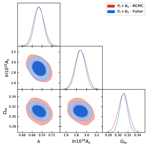
$\sigma(\cdot)$	$h$	$\ln(10^{10}A_{s})$	$\Omega_{m}$
$P_{\ell}+B_{0}\text{ - MCMC}$	0.011	0.11	0.011
$P_{\ell}+B_{0}\text{ - Fisher}$	0.0093	0.094	0.008

Figure 1: Triangle plots and errors comparing a Fisher forecast (blue) against the data analysis from [110] (red) for base $\Lambda$CDM parameters. For the Fisher forecast the full measured covariance is used including all cross-correlations. We here analyze $\ell=0,2$ power spectrum multipoles and the bispectrum monopole, both at one loop order. We implement the approximate AP effect as discussed in Sec. 2.4.

We observe that the largest discrepancy in the $\sigma$, at $27\%$, is found for $\Omega_{m}$. However, for the other cosmological parameters, the difference is only around $15\%$. We expect a similar level of error, at approximately $15\%$, for the other parameters that we analyze in the following sections and attribute the higher discrepancy on $\Omega_{m}$ to not fully modelling the AP effect, which most notably depends on $\Omega_{m}$. However, as argued above this effect will not be relevant for us in later sections. We note that if we remove the AP effect and window functions from the BOSS data analysis, the difference to the forecast is less than 5% .

3.2 Fisher prediction with diagonal covariance

For upcoming surveys, the fully measured covariance from mocks is not readily available. Although it is possible to compute these covariances with high accuracy using perturbation theory, the modeling of off-diagonal contributions can be very complex. Therefore, as described in Sec. 2, we do not consider any off-diagonal contributions here . Explicitly this means we neglect cross-correlations between the power spectrum and bispectrum and also we neglect cross-correlations between $k$-bins (for the power spectrum and bispectrum respectively) .

By considering the diagonal elements of the measured covariance (actively putting the off-diagonal elements to zero), we can study two effects. First, we can better understand the contribution of off-diagonal elements to the covariance, without yet relying on perturbation theory. Secondly, we can investigate the precision of the analytical diagonal covariance as described in Sec. 2 by comparing them to the diagonals of the measured covariance.

The most significant effect of using a diagonal covariance is an overestimation of the bispectrum impact relative to the power spectrum. We find that the off-diagonal elements in the power spectrum covariance have a negligible effect. However, for the bispectrum, the impact is larger. This is expected, as neglecting the power spectrum-bispectrum cross-correlation is equivalent to a scenario where the bispectrum is providing purely independent, new, information from the power spectrum. At least on large enough scales, this is inaccurate as discussed in [115]. In that sense, neglecting the cross-covariance is a double counting of large-scale information. Keeping this in mind, we still want to emphasize that the relative impact of the bispectrum grows rapidly with higher $k_{\text{max}}$.

In Fig. 2, we show the impact of these two isolated effects. First, by reducing the full covariance to just the diagonals, we obtain about $25\%-30\%$ tighter constraints. Second, if we compare the measured diagonal covariance to the modeled one, the agreement is remarkably good with only a few percent difference . In fact, this could be accounted for by loop order contributions that we did not consider in our analytic modeling of the diagonal covariance which is roughly of the same order.

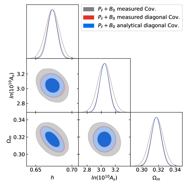
$\sigma(\cdot)$	$h$	$\ln(10^{10}A_{s})$	$\Omega_{m}$
$P_{\ell}+B_{0}\text{ measured Cov.}$	0.0093	0.094	0.008
$P_{\ell}+B_{0}\text{ measured diagonal Cov.}$	0.0070	0.066	0.0061
$P_{\ell}+B_{0}\text{ analytical diagonal Cov.}$	0.0065	0.064	0.0059

Figure 2: Triangle plots comparing different Fisher forecasts for base $\Lambda$CDM parameters using the $\ell=0,2$ power spectrum multipoles and the bispectrum monopole, all at one loop order. The plots differ only in their covariances, where we compare the measured covariance (grey) including all cross-covariances, the diagonal of the measured covariance (red), and the analytical prediction for the diagonal covariance (blue). We implement the approximate AP effect as discussed in Sec. 2.4.

By comparing the MCMC data analysis in Fig. 1 to the Fisher forecast using the analytical diagonal covariance shown in Fig. 2, we estimate our confidence in the Fisher results to be about $40\%$.

Finally, we perform the same comparison for non-Gaussianity constraints. The MCMC data analysis yields $\left(\sigma(f_{\text{NL}}^{\text{loc.}}),\sigma(f_{\text{NL}}^{\text{eq.}}),\sigma(f_{\text{NL}}^{\text{orth.}})\right)$= (35, 298, 75), while the Fisher forecast with analytical diagonal covariance gives $\left(\sigma(f_{\text{NL}}^{\text{loc.}}),\sigma(f_{\text{NL}}^{\text{eq.}}),\sigma(f_{\text{NL}}^{\text{orth.}})\right)$= (28, 275, 95). Thus for non-Gaussianity, we have a much closer agreement at around $10-25\%$.

4 Results

Having validated the Fisher methodology with BOSS data analysis results in Sec. 3, we now use it to predict the constraining power of DESI and MegaMapper, as well as to provide some additional results for BOSS. As discussed in the previous section, due to observational effects and covariance modeling, we expect the accuracy of cosmological parameter constraints to be roughly $40\%$, and the non-Gaussianity parameters to be accurate to $10-25\%$.

While BOSS has now been extensively analyzed, there are still some unexplored questions, which we aim to address here. The full set of cosmological parameters we study in various combinations is $\{h,\ln(10^{10}A_{s}),\Omega_{m},n_{s},\Omega_{k},\log m_{\nu}^{\text{tot.}},f_{\text{NL}}^{\text{loc.}},f_{\text{NL}}^{\text{eq.}},f_{\text{NL}}^{\text{orth.}}\}$, where we defined $\log m_{\nu}^{\text{tot.}}:=\log(\sum_{i}m_{\nu_{i}}/\text{eV})$. We refer to any subset of the first six parameters in this list (i.e. the list without the non-Gaussianity parameters) as “base” parameters. Throughout this section, we use the power spectrum and bispectrum of galaxies in redshift space at 1-loop order. For future surveys like DESI and MegaMapper, we use the full set of multipoles , and for BOSS we use either the full set of multipoles or the monopole and quadrupole for the power spectrum and the monopole for the bispectrum . Furthermore, following the discussion in Sec. 2.3, we fix the leading stochastic terms to one, throughout this section. Therefore, the results we will find for BOSS in this section are slightly tighter than what we presented in Sec. 3. When quoting results for primordial non-Gaussianity, we fix the cosmological parameters, as we will discuss more later this has almost always a negligible effect on our results. Finally, we note that we use fixed relationships from [28, 120] between the non-Gaussianity bias parameters $b_{i}^{f_{\text{NL}}}$ and galaxy bias parameters $b_{i}$, which we checked to be a negligible approximation with respect to putting an order one prior centered on $b_{i}^{f_{\text{NL},\text{ref}}}$ on $b_{i}^{f_{\text{NL}}}$ and then let it vary freely .

4.1 BOSS

Base cosmological results with the one-loop power spectrum for BOSS have been presented in [3, 4, 5], neutrinos have also been analyzed in [5] and dark energy models in [19]. The combination of the power spectrum and bispectrum has led to the measurement of $h$, $\ln(10^{10}A_{s})$ and $\Omega_{m}$ in [110], with the non-Gaussian parameter $f_{\rm{NL}}$ being reported in [28] and at tree level in [29, 34]. In this section, we present forecasts for the power spectrum and bispectrum with the inclusion of the sum of neutrino masses $\sum_{i}m_{\nu_{i}}$, spectral tilt $n_{s}$ and spatial curvature $\Omega_{k}$. We also investigate the impact of shot noise and of the EFT parameters and explore the information contained in higher multipoles. The exact numerical values of the EFT parameters, survey specification and reference cosmology that we use here and in Sec. 5 are given in App. A. Following the binning scheme used in [87], we divide the sample into two redshift bins. We use the same values of $k_{\text{NL}}$ and $b_{1}$ for both bins since the redshift difference of the bins is very small. The effective numbers we use are summarized in Tab. 1.

BOSS:	$z_{\text{eff}}$	$n_{b,\text{eff}}[(h\,{\rm Mpc}^{-1})^{3}]$	$b_{1}^{\text{ref}}$	($k^{\text{Tree}}_{\rm max}$, $k^{1L}_{\rm max}$, $k_{\text{NL}}$) $[h\,{\rm Mpc}^{-1}]$	$N^{1L}_{\text{bins}}$	$N^{\text{Tree}}_{\Delta}$	$N^{1L}_{\Delta}$
Bin 1	0.32	2.9$\times 10^{-3}$	1.9	(0.09, 0.20, 0.7)	18	9	62
Bin 2	0.57	2.5$\times 10^{-3}$	1.9	(0.10, 0.22, 0.7)	21	17	150

Table 1: BOSS effective survey specifications, calculated according to the formulas in Sec. 2 and Tab. 5 in App. A. $n_{b,\text{eff}}$ is the background galaxy number density entering the derivatives (not the covariance), $N_{\text{bins}}$ is the number of $k$-bins we consider for the power spectrum and $N_{\Delta}$ is the number of triangles we consider for the bispectrum.

This section is divided into two parts, based on the type of covariance used. In the first part, we present results using the full measured covariance obtained in [110], which includes all cross-correlations. This implies that we expect our results to be accurate to about $15\%$ (and $27\%$ for $\Omega_{m}$) as described in Sec. 3.1. In the second part, we investigate the impacts of shot noise and higher multipoles using a modeled covariance, as described in Sec. 3.2. This allows us to have better analytical control, for example in order to analyze the shot noise influence on the results.

Additional results: $n_{s}$, $\sum_{i}m_{\nu_{i}}$ and $\Omega_{k}$

We present the BOSS forecasts using the power spectrum monopole and quadrupole, as well as the bispectrum monopole, both at one loop order, for parameters that have previously only been analyzed with only the power spectrum (and in some cases with the tree-level bispectrum [3]). The results are summarized in Fig. 3.

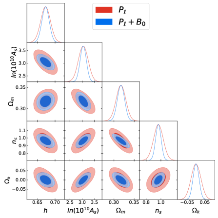
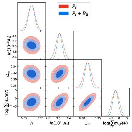
$\sigma(\cdot)$	$h$	$\ln(10^{10}A_{s})$	$\Omega_{m}$	$n_{s}$	$\Omega_{k}$
$P_{\ell}$	0.014	0.2	0.012	0.066	0.027
$P_{\ell}$+$B_{0}$	0.01	0.13	0.009	0.037	0.017

$\sigma(\cdot)$	$h$	$\ln(10^{10}A_{s})$	$\Omega_{m}$	$\log m_{\nu}^{\text{tot.}}({}^{\sigma^{+}}_{\sigma^{-}})$
$P_{\ell}$	0.011	0.14	0.011	2.3 (${}^{+0.84}_{-0.089}$)
$P_{\ell}$+$B_{0}$	0.0092	0.095	0.008	1.6 (${}^{+0.41}_{-0.080}$)

$\sigma(\cdot)$	$f_{\text{NL}}^{\text{loc.}}$	$f_{\text{NL}}^{\text{eq.}}$	$f_{\text{NL}}^{\text{orth.}}$
$P_{\ell}$+$B_{0}$	25	266	94

Figure 3: Triangle plots and errors from Fisher forecasts for BOSS including the spectral tilt and spatial curvature (left), massive neutrinos (right), and primordial non-Gaussianity (bottom). The power spectrum monopole and quadrupole, and the bispectrum monopole were used both at one loop order. In the table we also report the upper and lower bounds of the $68\%$ confidence interval for the sum of massive neutrinos, i.e $\mathbb{P}\left[\left(\sum_{i}m_{\nu_{i}}-\sum_{i}m_{\nu_{i}}^{\text{ref}}\right)\in(\sigma^{-},\sigma^{+})\right]=0.68$. The covariance used here is the full, measured covariance with all cross-correlations. We implemented the approximate AP effect as discussed in Sec. 2.4.

Impact of shot noise, biases and multipoles

For BOSS, we checked that adding the trispectrum at tree level and the 2-loop power spectrum  do not improve on the measurements . This is mostly attributable to the large shot noise of the survey. However, given the power of the Fisher formalism, we can investigate the effects of certain limits and configurations on parameter constraints. Of course, we here look at limiting cases, that are unrealistic in reality, but they show where information is lost. In particular, we are interested in the impact of EFT parameters and of the survey shot noise. Throughout this section, we will be using the analytical covariance, which gives us the most control but comes with the caveats mentioned in Sec. 3. We investigate several effects on both base cosmological parameters including $n_{s}$, and $f_{\text{NL}}$. Just as in [28], unless mentioned otherwise, we fix the cosmological parameters when quoting errors on $f_{\text{NL}}$. We checked that while $f_{\text{NL}}^{\text{loc.}}$ has a roughly 35% error bar reduction due to fixed cosmological parameters, $f_{\text{NL}}^{\text{eq.}}$ and $f_{\text{NL}}^{\text{orth.}}$ are very independent of the other cosmological parameters and their results would only change by roughly $5-10\%$ if we would not fix the cosmological parameters.

First, we check the impact of using higher multipoles at one loop as opposed to using only the power spectrum monopole and quadrupole and the bispectrum monopole. While there is some improvement with the inclusion of additional multipoles for the bispectrum, we checked that almost all of this improvement comes from the bispectrum quadrupoles. Still, this improvement is very small, and so we do not present the posteriors. The numerical values can be found in the table of Fig. 4. We can conclude that using the monopole and quadrupole for both the power spectrum and bispectrum, one can extract almost the full redshift space information. As was shown in [110, 28], we can already analyze data with the monopole and quadrupole for the power spectrum and bispectrum. Therefore, unless indicated otherwise we analyze using all multipoles.

Next in Fig. 4, we show additional constraints in the continuous field limit $n_{b}\rightarrow\infty$, i.e. having no shot noise. We roughly halve the error bars for both the base cosmological parameters and $f_{\text{NL}}$. This should serve as motivation to include as many objects into our data sets even if they are faint or somewhat unresolved. This will also become important in Sec. 4.3.

Lastly, the EFTofLSS, like any EFT, will need a larger number of parameters when going to higher perturbative orders. This is in principle not a problem as long as they are independent enough from the parameters of interest. It is interesting to investigate how better knowledge of these parameters would impact the results. We put the “galaxy-formation prior” mentioned in Sec. 2.4, where we put stronger priors on all EFT parameters motivated by hopefully-realistic future knowledge on galaxy formation. We also take the limit in which these parameters are fixed, in other words representing the scenario in which all “nuisance” parameters are known and measured exactly with no error. This, in a sense, is the theoretical upper bound for the EFTofLSS at a given order. It is interesting to note from the results presented in the table in Fig. 4 that the biases have varying impacts on different cosmological parameters. Specifically, the biases overwhelmingly affect the primordial parameters, $A_{s},n_{s}$ and $f_{\text{NL}}$. As we will see in Sec. 5, $f_{\text{NL}}$-constraints are more sensitive to the EFT parameters than $A_{s}$ and $n_{s}$. This is not so surprising, considering that the functional form of EFT counterterms resemble the functional form induced by primordial non-Gaussianities.

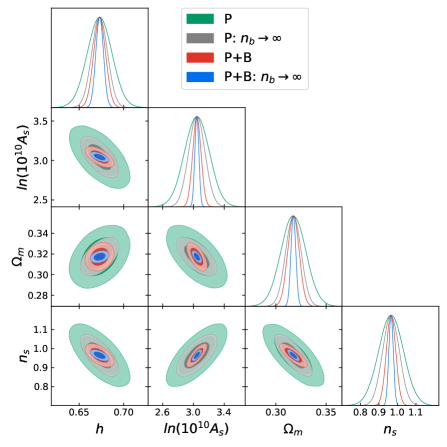
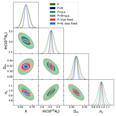
$\sigma(\cdot)$	$h$	$\ln(10^{10}A_{s})$	$\Omega_{m}$	$n_{s}$	$f_{\text{NL}}^{\text{loc.}}$	$f_{\text{NL}}^{\text{eq.}}$	$f_{\text{NL}}^{\text{orth.}}$
$P_{\ell}$	0.014	0.16	0.012	0.067	-	-	-
$P$	0.014	0.16	0.012	0.067	-	-	-
$P+g.p.:$	0.013	0.13	0.011	0.047	-	-	-
$P:$ bias fixed	0.012	0.06	0.008	0.026	-	-	-
$P:n_{b}\rightarrow\infty$	0.009	0.11	0.008	0.045	-	-	-
$P_{\ell}$+$B_{0}$	0.0067	0.092	0.0060	0.029	25	266	94
$P$+$B$	0.0067	0.055	0.0057	0.025	23	253	67
$P+B+g.p.:$	0.0065	0.043	0.0049	0.019	19	187	51
$P+B:$ bias fixed	0.0054	0.019	0.0035	0.007	4.8	45	26
$P+B:n_{b}\rightarrow\infty$	0.0043	0.026	0.0024	0.012	11	147	41

Figure 4: Triangle plots and errors from several different Fisher forecasts for BOSS using the analytical covariance. We compare base results to results obtained without shot noise (left) and with biases fixed or with a “galaxy-formation prior” (g.p.) (right). In the table, we also show the impact of including higher multipoles on the power spectrum and bispectrum and also see the impact on $f_{\text{NL}}$. For the constraints on $f_{\text{NL}}$, we fix the other cosmological parameters.

4.2 DESI

We now turn to predict the performance of upcoming surveys, starting with the imminent DESI survey. We base our results on the Emission Line Galaxies (ELGs) sample, which is the largest of the DESI surveys [88]. We note that while we are able to derive the value for the linear bias through specifications given in [88], we do not have values for the other EFT parameters. We therefore shift all biases according to the method described in Sec. 2.3, i.e. we shift them all according to the change in the linear bias with respect to the BOSS best-fit. The final numerical values we use for the DESI forecast are given in Tab. 2. For all the future surveys we use $k_{\text{min}}=0.001h\,{\rm Mpc}^{-1}$ for the power spectrum and $k_{\text{min}}=0.02h\,{\rm Mpc}^{-1}$ for the bispectrum. We bin with $\Delta k=0.005h\,{\rm Mpc}^{-1}$ for the power spectrum and $\Delta k=0.02h\,{\rm Mpc}^{-1}$ for the bispectrum. For binning consistency, we have checked that using a smaller binning does not affect our results. To reduce binning effects, ideally one would always average the observables over a $k$-bin. However, given the numerical complexity of doing such a procedure for every bin, especially for the bispectrum, we instead evaluate on a effective number $k_{\text{eff}}$ to approximate this averaging. This is analogous to the method used for example in [110], with the difference that we also evaluate on $k_{\text{eff}}$ the tree level contribution, rather than averaging it. The effect is minimal. Throughout this section, we use the analytical covariance from Eq. (2.16) and Eq. (2.2) with all the ingredients discussed in Sec. 2.3. We remind that the validity of the covariance was discussed in Sec. 3.

DESI:	$z_{\text{eff}}$	$n_{b,\text{eff}}[(h\,{\rm Mpc}^{-1})^{3}]$	$b_{1}^{\text{ref}}$	($k^{\text{Tree}}_{\rm max}$, $k^{1L}_{\rm max}$, $k_{\text{NL}}$) $[h\,{\rm Mpc}^{-1}]$	$N^{1L}_{\text{bins}}$	$N^{\text{Tree}}_{\Delta}$	$N^{1L}_{\Delta}$
Bin 1	0.84	8.0$\times 10^{-4}$	1.3	(0.08, 0.18, 0.9)	37	17	115
Bin 2	1.23	3.2$\times 10^{-4}$	1.5	(0.09, 0.23, 1.3)	45	17	191

Table 2: DESI effective survey specifications, calculated according to the formulas in Sec. 2 and Tab. 6 in App. A. $n_{b,\text{eff}}$ is the background galaxy number density entering the derivatives (not the covariance), $N_{\text{bins}}$ is the number of $k$-bins we consider for the power spectrum and $N_{\Delta}$ is the number of triangles we consider for the bispectrum.

Results

We present results, including the spectral tilt, spatial curvature, neutrino masses, and non-Gaussianity in Fig. 5, using all multipoles. The results for $f_{\text{NL}}$ were obtained with fixed cosmological parameters. Analyzing $f_{\text{NL}}$ in combination with cosmological parameters changes the $f_{\text{NL}}$ constraints by less than 8%. For neutrino masses, with the caveats discussed in footnote 17, it seems likely that DESI is already able to detect massive neutrinos at the 2$\sigma$ level.

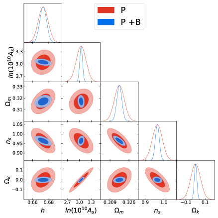
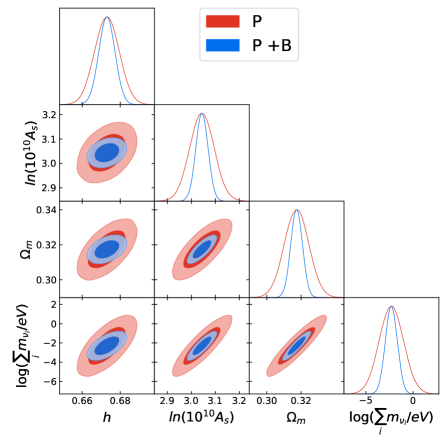
$\sigma(\cdot)$	$h$	$\ln(10^{10}A_{s})$	$\Omega_{m}$	$n_{s}$	$\Omega_{k}$
$P$	0.0061	0.12	0.0045	0.027	0.051
$P$+$B$	0.0042	0.035	0.0023	0.011	0.013

$\sigma(\cdot)$	$h$	$\ln(10^{10}A_{s})$	$\Omega_{m}$	$\log m_{\nu}^{\text{tot.}}({}^{\sigma^{+}}_{\sigma^{-}})$
$P$	0.0065	0.051	0.0072	1.3 (${}^{+0.26}_{-0.072}$)
$P$+$B$	0.0042	0.025	0.0034	0.63 (${}^{+0.087}_{-0.047}$)

$\sigma(\cdot)$	$f_{\text{NL}}^{\text{loc.}}$	$f_{\text{NL}}^{\text{eq.}}$	$f_{\text{NL}}^{\text{orth.}}$
$P$+$B$	3.5	114	30

Figure 5: Triangle plots and errors from Fisher forecasts for DESI including the spectral tilt and spatial curvature (left) and massive neutrinos (right) and Non-Gaussianity (bottom). In the table we also report the upper and lower bounds of the $68\%$ confidence interval for the sum of massive neutrinos, i.e $\mathbb{P}\left[\left(\sum_{i}m_{\nu_{i}}-\sum_{i}m_{\nu_{i}}^{\text{ref}}\right)\in(\sigma^{-},\sigma^{+})\right]=0.68$. We use all power spectrum and bispectrum multipoles at one loop order for the above results and use the analytical covariance without cross-correlations.

Impact of shot noise and biases

Similar to Sec. 4.1, it is interesting to investigate constraints with the “galaxy-formation prior” (g.p.) putting stronger priors on EFT parameters, and look at the theoretical limits of fixed biases and zero shot noise for DESI. As shown in Fig. 6, the g.p. mostly affects $f_{\text{NL}}^{\text{eq.}}$ and $f_{\text{NL}}^{\text{orth.}}$. However, in both the zero shot noise  and fixed bias limits, we observe improvements of roughly a factor of 2-3 in $\ln(10^{10}A_{s}),\Omega_{m}$ and $n_{s}$, while $h$ improves less significantly in either of these limits. These results are consistent with those obtained for BOSS in Sec. 4.1 since, as we noted, the biases have larger degeneracies with $\ln(10^{10}A_{s})$, $n_{s}$, and non-Gaussianities. We find that the effect of shot noise accounts for approximately 50% of the constraints on $f_{\text{NL}}$. Interestingly, fixing the bias parameters has a striking effect on non-Gaussianities, particularly for $f_{\text{NL}}^{\text{eq.}}$, for which we would obtain a six-fold reduction in the error bars. In combination with the results from the g.p., this strongly motivates the need for tighter priors and therefore better measurements of biases when performing the analysis of DESI in the near future. In order to further improve on this aspect, we present in Sec. 5 the $f_{\text{NL}}$ constraints forecasted with the EFT-motivated perturbativity prior.

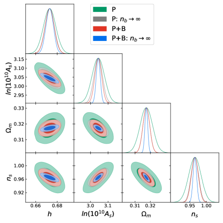
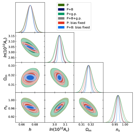
$\sigma(\cdot)$	$h$	$\ln(10^{10}A_{s})$	$\Omega_{m}$	$n_{s}$	$f_{\text{NL}}^{\text{loc.}}$	$f_{\text{NL}}^{\text{eq.}}$	$f_{\text{NL}}^{\text{orth.}}$
$P$	0.0057	0.036	0.0041	0.019	-	-	-
$P+g.p.:$	0.0056	0.032	0.0040	0.016	-	-	-
$P:$ bias fixed	0.0053	0.021	0.0032	0.011	-	-	-
$P:n_{b}\rightarrow\infty$	0.0044	0.024	0.0022	0.011	-	-	-
$P$+$B$	0.0042	0.020	0.0022	0.010	3.5	114	30
$P+B+g.p.:$	0.0042	0.018	0.0022	0.009	3.4	83	23
$P+B:$ bias fixed	0.0037	0.010	0.0016	0.004	2.0	21	11
$P+B:n_{b}\rightarrow\infty$	0.0035	0.011	0.0009	0.005	1.7	67	17

Figure 6: Triangle plots and errors from several different Fisher forecasts for DESI. We compare base results to results obtained without shot noise (left) and with biases fixed or with a “galaxy-formation prior” (g.p.) (right). In the table, we also show the impact of including higher multipoles on the power spectrum and bispectrum and also see the impact on $f_{\text{NL}}$. For the constraints on $f_{\text{NL}}$, we fix the other cosmological parameters.

4.3 MegaMapper

For MegaMapper, we base our Fisher forecasts on the two scenarios mentioned in [89] (there called “idealized” and “fiducial”), which we call the optimistic (MMo) and pessimistic (MMp) scenarios. These two scenarios are in turn based on the specifications presented in Tab. 1 (MMo) and Tab. 2 (MMp) of [117]. It is important to note that these specifications are preliminary and may differ from the final specifications. We caution that our results are based on these preliminary specifications and may need to be revised as more information becomes available. We find that the constraints predicted by the two scenarios differ by $30-40\%$. Given the similarity of the results in these two situations, we present here the results in the optimistic scenario, leaving the pessimistic scenario in App. B.1. Thus, the numerical values that we will use in this section were derived from Tab. 1 of [117] and methods from Sec. 2. They are given in Tab. 3.

MMo:	$z_{\text{eff}}$	$n_{b,\text{eff}}[(h\,{\rm Mpc}^{-1})^{3}]$	$b_{1}^{\text{ref}}$	($k^{\text{Tree}}_{\rm max}$, $k^{1L}_{\rm max}$, $k_{\text{NL}}$) $[h\,{\rm Mpc}^{-1}]$	$N^{1L}_{\text{bins}}$	$N^{\text{Tree}}_{\Delta}$	$N^{1L}_{\Delta}$
Bin 1	2.4	1.8$\times 10^{-3}$	3.1	(0.14, 0.36, 3.2)	73	62	696
Bin 2	4.3	1.1$\times 10^{-4}$	6.3	(0.28, 0.76, 10.1)	153	294	5491

Table 3: MegaMapper effective survey specifications, calculated according to the formulas in Sec. 2 and Tab. 7 in App. A. $n_{b,\text{eff}}$ is the background galaxy number density entering the derivatives (not the covariance), $N_{\text{bins}}$ is the number of $k$-bins we consider for the power spectrum at 1-loop and $N_{\Delta}$ is the number of triangles we consider for the bispectrum at 1-loop.

As in the DESI forecast, we shift the rest of the biases parameters according to the method described in Sec. 2.3. Furthermore, we again use $k_{\text{min}}=0.001h\,{\rm Mpc}^{-1}$ for the power spectrum and $k_{\text{min}}=0.02h\,{\rm Mpc}^{-1}$ for the bispectrum, as well as $\Delta k=0.005h\,{\rm Mpc}^{-1}$ for the power spectrum and $\Delta k=0.02h\,{\rm Mpc}^{-1}$ for the bispectrum. Again, to reduce binning effects, we evaluate on $k_{\text{eff}}$. The results for $f_{\text{NL}}$ were again obtained with fixed cosmological parameters. Analyzing $f_{\text{NL}}$ in combination with cosmological parameters changes the $f_{\text{NL}}$ constraints by less than 3%. Finally, just like for the DESI forecasts, we use the analytical covariance from Eq. (2.16) and Eq. (2.2), following the discussion in Sec. 2.3 and its precision discussed in Sec. 3.

Results

We present base results for MegaMapper in a similar format to the previous sections in Fig. 7. We see that the bispectrum contains significant constraining power. As mentioned in Sec. 3.2, we expect that the constraints presented here will be an overestimate as we are neglecting cross-correlations. Nevertheless, the impact of the bispectrum at higher $k_{\rm max}$ becomes relatively more important, and therefore continues to be a very important tool for future data analyses.

In particular, shown in in Fig. 7, the inclusion of the bispectrum allows for very tight constraints on neutrino masses. Even with the caveats discussed in footnote 17, neutrino mass detection with MegaMapper seems very likely.

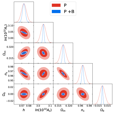
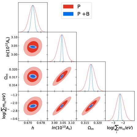
$\sigma(\cdot)$	$h$	$\ln(10^{10}A_{s})$	$\Omega_{m}$	$n_{s}$	$\Omega_{k}$
$P$	0.0036	0.021	0.0012	0.006	0.0076
$P+B$	0.0021	0.0052	0.0003	0.002	0.0015

$\sigma(\cdot)$	$h$	$\ln(10^{10}A_{s})$	$\Omega_{m}$	$\log m_{\nu}^{\text{tot.}}({}^{\sigma^{+}}_{\sigma^{-}})$
$P$	0.0023	0.022	0.0015	0.38 (${}^{+0.046}_{-0.031}$)
$P$+$B$	0.0010	0.0039	0.0004	0.083 (${}^{+0.009}_{-0.008}$)

$\sigma(\cdot)$	$f_{\text{NL}}^{\text{loc.}}$	$f_{\text{NL}}^{\text{eq.}}$	$f_{\text{NL}}^{\text{orth.}}$
$P$+$B$	0.27	17.7	4.6

Figure 7: Triangle plots and errors from Fisher forecasts for MegaMapper including the spectral tilt and spatial curvature (left) and massive neutrinos (right) and non-Gaussianity (bottom). In the table we also report the upper and lower bounds of the $68\%$ confidence interval for the sum of massive neutrinos, i.e $\mathbb{P}\left[\left(\sum_{i}m_{\nu_{i}}-\sum_{i}m_{\nu_{i}}^{\text{ref}}\right)\in(\sigma^{-},\sigma^{+})\right]=0.68$. We use all power spectrum and bispectrum multipoles for the above results and use the analytical covariance without cross-correlations.

Impact of shot noise and biases

Given the long timeline until results will be available for MegaMapper, and target selection is yet to happen, we will discuss some aspects that might improve results as was discussed for DESI in Sec. 4.2. In particular, while the perturbative reach is far greater at higher redshifts, as can be seen from Tab. 8, the shot noise, especially for the higher redshift bin, is extremely large . We, therefore, present the limiting case of zero shot noise to better understand the possible gain achievable by reducing the currently estimated shot noise. Equally motivated by the long timeline of MegaMapper, we present results with stronger bias priors, anticipating the better understanding of galaxy formation until the data release. Along with the zero shot noise and “galaxy-formation prior” results, we also present the impact of fixing biases in Fig. 8.

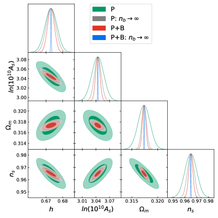
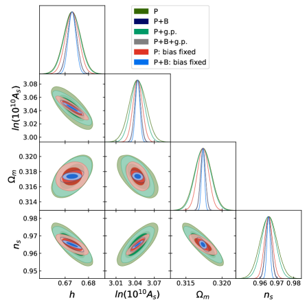
$\sigma(\cdot)$	$h$	$\ln(10^{10}A_{s})$	$\Omega_{m}$	$n_{s}$	$f_{\text{NL}}^{\text{loc.}}$	$f_{\text{NL}}^{\text{eq.}}$	$f_{\text{NL}}^{\text{orth.}}$
$P$	0.0036	0.013	0.0012	0.005	-	-	-
$P+g.p.:$	0.0034	0.011	0.0011	0.0043	-	-	-
$P:$ bias fixed	0.0029	0.0074	0.00079	0.0024	-	-	-
$P:n_{b}\rightarrow\infty$	0.0029	0.0074	0.00047	0.0029	-	-	-
$P$+$B$	0.0021	0.0047	0.00034	0.0017	0.27	18	4.6
$P+B+g.p.:$	0.0020	0.0045	0.00033	0.016	0.26	13	3.6
$P+B:$ bias fixed	0.0016	0.0034	0.00021	0.0010	0.17	3.6	1.7
$P+B:n_{b}\rightarrow\infty$	0.00019	0.00045	0.000029	0.00018	0.11	5.4	1.5

Figure 8: Triangle plots and errors from several different Fisher forecasts for MegaMapper. We compare base results to results obtained without shot noise (left) and with biases fixed or with a “galaxy-formation prior” (g.p.) (right). In the table, we also show the impact of including higher multipoles on the power spectrum and bispectrum and also see the impact on $f_{\text{NL}}$. For the constraints on $f_{\text{NL}}$, we fix the other cosmological parameters.

We see that stronger bias priors mostly have an effect on $f_{\text{NL}}^{\text{eq.}}$ and $f_{\text{NL}}^{\text{orth.}}$. Going further and fixing the biases we would again, roughly, reduce the error bar by a factor 2, with again the exception of $f_{\text{NL}}^{\text{eq.}}$ where the dependence is much stronger. This again motivates the perturbativity prior we discuss in Sec. 5. This is very similar to the case of BOSS and DESI shown in Secs. 4.1 and 4.2. Thus, the relative gain of putting the “galaxy-formation prior” or fixing the biases is very similar among the three surveys we consider.

However, shot noise affects the three surveys very differently. In particular, for MegaMapper, shot noise is quite significant for some cosmological parameters. Especially for the base parameters, we can see from the table in Fig. 8, that reduction of shot noise for MegaMapper can lead to a $\sim$10-fold error bar reduction. Instead for non-Gaussianity parameters, while shot noise still seems to be in an important factor, it is comparably less significant. In particular, the effect of setting shot noise to zero is similar to fixing the biases when analyzing $f_{\text{NL}}$.

5 Further constraining $f_{\text{NL}}$ with a perturbativity prior

As we have seen in Sec. 4, in particular Figs. 4, 6 and 8, fixing the biases leads to stronger constraints on the primordial parameters $\ln(10^{10}A_{s})$ and $n_{s}$ and to vast improvements on some $f_{\text{NL}}$ parameters. We will see in this section that some non-Gaussianity parameters are greatly affected by EFT parameter constraints. In particular, small improvements on the constraints on the bias parameters can lead to significant improvements on $f_{\text{NL}}^{\text{eq.}}$ and $f_{\text{NL}}^{\text{orth.}}$. We are thus motivated to place stronger (and physically justifiable) priors on the nuisance parameters in order to further constrain single-field inflation.

As mentioned in Sec. 2.3, we put independent priors on the EFT parameters, restricting their individual size. This is motivated by the fact that the EFTofLSS predicts these parameters to be of order one. However, given that the MCMC explores the full parameter space in a random walk, the final loop contribution can be $\sqrt{n}$ larger than the truth, where $n$ is the number of EFT parameters. We aim to address the issue that such parameter configurations are unphysical yet can still fit the data well. This happens because, at intermediate and low $k$’s, where each term is not too small, even a too-large loop is comparably small with respect to the data error that scales like $k^{-3/2}$. Therefore, only at large $k$ where the data error is sufficiently small, would parameter configurations exhibiting $\sqrt{n}$ enhancements to the loop be ruled out. However, there exist parameter configurations exhibiting $\sqrt{n}$ larger contributions at lower $k$’s that cancel out at large $k$, making the loop appear to have the correct size at those scales. Therefore, a loop contribution that is too large at low $k$ can still fit the data well, but would go unnoticed, even though it would clearly be unphysical. Through scaling relations, this then translates to an overestimate of the expected higher loop contribution. This argument is shown for the estimated 2-loop contribution in Fig. 9.

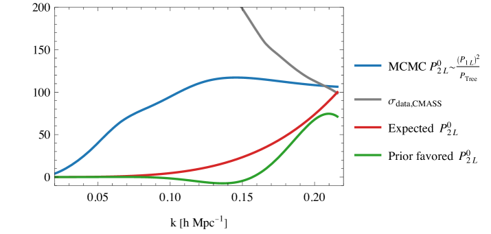
Figure 9: Plot showing various two-loop monopole power spectra, $P_{2L}^{0}$ against the CMASS data error, $\sigma_{\text{data,CMASS}}$ (grey). As an example of a typical MCMC, the BOSS CMASS $P_{2L}^{0}$ was estimated using the relation $P_{2L}\sim\frac{P^{2}_{1L}}{P^{\rm Tree}}$, and is shown in blue. The expected $P_{2L}^{0}$ size is shown in red and an example of a $P_{2L}^{0}$ that would be favoured by the perturbativity prior is shown in green.

We, therefore, propose an additional prior, which we call “perturbativity prior”, on the size of the loop contributions, aimed at being effective in the intermediate and low $k$ regions where the $\sqrt{n}$ enhancements are not sufficiently restricted by the data analysis. To formulate this “perturbativity prior”, we use the fact that, as we sample the different bias configurations, the two-loop contribution can have a maximal size, and therefore a maximal signal-to-noise. This maximal signal-to-noise was what defined the $k_{\text{max}}$ in Eq. (2.22). In this section, we show that by using appropriate scaling relations between the two-loop and one-loop contributions, we can translate this threshold for the two-loop contribution into a prior on the size of the one-loop contribution.

5.1 Contribution to the Fisher matrix

We impose a perturbativity prior for the power spectrum and bispectrum respectively, and the procedure is the same in both cases. We therefore keep the derivation generic, for the loop of some observable, $X_{1L}$, where $X\in\{P,B\}$. In a later step, we will derive an estimate for the correct size of the loop, denoted by $X_{1L}^{C}$. As mentioned in the previous section, this estimate will come from a threshold for the signal-to-noise of two-loop contributions, through which we can infer properties about the correct one-loop contributions. The quantity we want to constrain is $X_{1L}$, whereas $X_{1L}^{C}$ we assume to be estimated before the data analysis. We then impose that on average, $X_{1L}$ is close to $X_{1L}^{C}$, therefore, we impose a Gaussian prior

$$\frac{1}{N_{X}}\sum_{k_{i}}\int_{-1}^{1}\int_{0}^{2\pi}\frac{d\mu_{i}}{2}\frac{d\phi}{2\pi}\frac{X_{1L}(k_{i};\hat{z})}{X_{1L}^{C}(k_{i};\hat{z})}\sim\mathcal{N}(1,1),$$ (5.1)

where $k_{i}\in\{k,(k_{1},k_{2},k_{3})\}$, $\mu_{i}\in\{\mu,\mu_{1}\}$ and $N_{X}\in\{N_{\text{bins}},N_{\Delta}\}$ for the power spectrum and bispectrum respectively. We here implement the real space part of the perturbativity prior . For the remainder of this section, we, therefore, always refer to real space quantities, indicated by dropping the $\hat{z}$ argument. The real space prior we then impose is given by

$$\frac{1}{N_{X}}\sum_{k_{i}}\frac{X_{1L}(k_{i})}{X_{1L}^{C}(k_{i})}\sim\mathcal{N}(1,1).$$ (5.2)

One way to write the prior above is to impose the same, independent, prior for each bin. That is, we impose

$$X_{1L}(k_{i})\sim\mathcal{N}\left(X_{1L}^{C}(k_{i}),N_{X}\left(X_{1L}^{C}(k_{i})\right)^{2}\right),$$ (5.3)

which implies Eq. (5.2).

In order to use this prior for the Fisher matrix, we assume once again that our reference cosmology is accurate and we assume $X_{1L}^{\text{ref}}\simeq X_{1L}^{C}$ (). Then, for fixed $k_{i}$, similarly to Eq. (2.3), we can Taylor expand to get 

$$-2\log\text{Prior} = \frac{1}{N_{X}\left(X_{1L}^{C}\right)^{2}}\left(X_{1L}(\theta)-X_{1L}^{C}\right)^{2}+r_{1}$$

$$\simeq (\theta-\theta^{\text{ref}})^{T}F^{X,\text{pert.}}(\theta-\theta^{\text{ref}})+r_{1},$$

where $F^{X,\text{pert.}}_{ij}=\frac{1}{N_{X}\left(X_{1L}^{C}\right)^{2}}\frac{\partial X_{1L}}{\partial\theta_{i}}\frac{\partial X_{1L}}{\partial\theta_{j}}$ and $r_{1}$ is a parameter-independent constant. Therefore, summing over all bins, the perturbativity prior that we finally implement in the Fisher forecast is given by

$$F_{ij}^{\text{\text{pert.}}} = \frac{1}{N_{\text{bins}}}\sum_{k}\frac{1}{P_{1L}^{C}(k)^{2}}\frac{\partial P_{1L}(k)}{\partial\theta_{i}}\frac{\partial P_{1L}(k)}{\partial\theta_{j}}$$

$$\quad+\frac{1}{N_{\Delta}}\sum_{k_{1},k_{2},k_{3}}\frac{1}{B_{1L}^{C}(k_{1},k_{2},k_{3})^{2}}\frac{\partial B_{1L}(k_{1},k_{2},k_{3})}{\partial\theta_{i}}\frac{\partial B_{1L}(k_{1},k_{2},k_{3})}{\partial\theta_{j}}.$$

In order to be able to implement this prior, we need to derive the estimates for $P_{1L}^{C}$ and $B_{1L}^{C}$. We derive the threshold for the size of the 1-loop contributions from limiting the 2-loop signal-to-noise ratio. This is similar to how we determined the $k_{\text{max}}$ in Sec. 2.3. There, we demanded that the signal-to-noise of the 2-loop contribution for any new survey does not exceed its signal-to-noise of BOSS CMASS, where we know it is negligible. In particular, the maximal signal-to-noise that has previously been chosen in the data analysis to determine the $k_{\text{max}}$ was $\frac{1}{9}$, which is also what we use here. Explicitly,

$$\int_{0}^{k_{\text{max}}}\left(\frac{P_{2L}(k)}{\tilde{\sigma}_{P,\text{data}}(k)}\right)^{2}dk\simeq\frac{1}{9},$$ (5.6)

$$\int_{\nu_{B}}\left(\frac{B_{2L}(k_{1},k_{2},k_{3})}{\tilde{\sigma}_{B,\text{data}}(k_{1},k_{2},k_{3})}\right)^{2}dk_{1}dk_{2}dk_{3}\simeq\frac{1}{9},$$

where $\tilde{\sigma}_{X,\text{data}}$ here is defined as in Eq. (2.3), using that in the continuum limit we get $\Delta k\rightarrow dk$, and $\nu_{B}$ is the set of all triangles with maximal wavenumber smaller than or equal to $k_{\text{max}}$. We then get the estimates for the correct one-loop contributions, through the approximate size relations between two-loop and one-loop, $P_{2L}\sim\frac{{P^{C}_{1L}}^{2}}{P^{NS}_{\text{Tree}}}$ and $B_{2L}\sim\frac{{B^{C}_{1L}}P^{C}_{1L}}{P^{NS}_{\text{Tree}}}$ (). Finally, in order to perform the integrals in Eq. (5.6), we assume scaling functions $S^{X}(k_{i})$, defined by $\frac{S^{X}(k_{i})}{S^{X}(k_{\text{max}})}=\frac{X^{C}_{1L}(k_{i})}{X^{C}_{1L}(k_{\text{max}})}$ (), that should approximate the $k$ dependencies of $X^{C}_{1L}(k_{i})$. Plugging in the size relations and scaling approximation into Eq. (5.6), we can solve for the $X^{C}_{1L}(k_{i})$ to get

$$P_{1L}^{C}(k)=S^{P}(k)\left(9\int_{0}^{k_{\text{max}}}\left(\frac{S^{P}(k^{\prime})^{2}}{P^{NS}_{\text{Tree}}(k^{\prime})\tilde{\sigma}_{P,\text{data}}(k^{\prime})}\right)^{2}dk^{\prime}\right)^{-1/4},$$ (5.7)

$$B_{1L}^{C}=S^{B}(k_{1},k_{2},k_{3})\left(9\int_{\nu_{B}}\left(\frac{S^{B}(k_{1}^{\prime},k_{2}^{\prime},k_{3}^{\prime})}{\tilde{\sigma}_{B,\text{data}}(k_{1}^{\prime},k_{2}^{\prime},k_{3}^{\prime})}\frac{1}{3}\left(\frac{P_{1L}^{C}(k_{1}^{\prime})}{P^{NS}_{\text{Tree}}(k_{1}^{\prime})}+2p.\right)\right)^{2}dk_{1}^{\prime}dk_{2}^{\prime}dk_{3}^{\prime}\right)^{-1/2},$$

where we dropped the $k$-dependence for $B_{1L}^{C}$ to avoid clutter and in the bottom line we symmetrize the $\frac{P_{1L}^{C}}{P^{NS}_{\text{Tree}}}$. Note that $P_{1L}^{C}$ and $B_{1L}^{C}$ do not depend on the overall size of the scaling estimates $S^{X}$, as we are normalizing it at $k_{\rm max}$.

There are well established estimates for the behaviour of the power spectrum loop [40] and bispectrum loop [122] in a scaling universe. For biased tracers we adapt this to

$$S^{P}_{\text{int}}(k) = P_{\text{Tree}}(k)\left(\frac{k}{k_{\text{NL}}}\right)^{3+n(k)},$$ (5.8)

$$S^{B}_{\text{int}}(k_{1},k_{2},k_{3}) = B_{\text{Tree}}(k_{1},k_{2},k_{3})\left(\left(\frac{k_{1}}{k_{\text{NL}}}\right)^{3+n(k_{1})}+2p.\right),$$

which is very similar to the one used in Eq. (2.23), but with $P_{\text{Tree}}$ and $B_{\text{Tree}}$ being the (real space) biased tracers tree-level power spectrum and bispectrum. In order to have both the right IR and UV behaviour of the loop contributions we also include a loop counter term to the estimate. For the scaling of the counterterms, we use

$$S^{P}_{c}(k) = -2b_{1}\beta P_{11}(k)\left(\frac{k}{k_{\text{NL}}}\right)^{2},$$ (5.9)

$$S^{B}_{c}(k_{1},k_{2},k_{3}) = -2b_{1}^{2}\beta\left(P_{11}(k_{1})P_{11}(k_{2})\left(\frac{k_{3}}{k_{\text{NL}}}\right)^{2}+2p.\right),$$

where we use the reference value $\beta_{\text{BOSS}}=1$ and rescale with Eq. (2.19) for other surveys . Finally, given that $S^{P}$ and $S^{B}$ should be upper bounds on the the scaling of the loops, we want to avoid cancelations and ensure positivity. Therefore, the final scalings we implement are

$$S^{P}(k) = \max(|S^{P}_{\text{int}}(k)|,|S^{P}_{c}(k)|),$$ (5.10)

$$S^{B}(k_{1},k_{2},k_{3}) = \max(|S^{B}_{\text{int}}(k_{1},k_{2},k_{3})|,|S^{B}_{c}(k_{1},k_{2},k_{3})|).$$

5.2 Results

While the perturbativity prior further constrains both cosmological parameters and bias parameters, the largest effect comes from further constraining particular bias parameters. We present this improvement in Fig. 10. Indeed, there we can see that small improvements on particular EFT parameters  lead to vast improvements on $f_{\text{NL}}^{\text{eq.}}$. In the tables of Fig. 10 we also show the effect on the other types of non-Gaussianity we analyze. Each analysis was performed with fixed cosmological parameters and each type of non-Gaussianity was analyzed separately. For completeness, and to stress the importance of the bispectrum loop, we also compare it with bispectrum tree-level constraints. The survey specifications used for the tree-level analysis are also in Tabs. 1, 2, and 3. In the following, we will present results for each survey based on the plots in Fig. 10.

Finally, as we also discussed in Sec. 4, base cosmological parameters are less affected by constraints on bias parameters. However, we find that the inclusion of the perturbativity prior can have a relevant effect on them, which we discuss in App. B.2. In particular, we find that DESI will constrain curvature to 0.012 and MegaMapper to 0.0012.

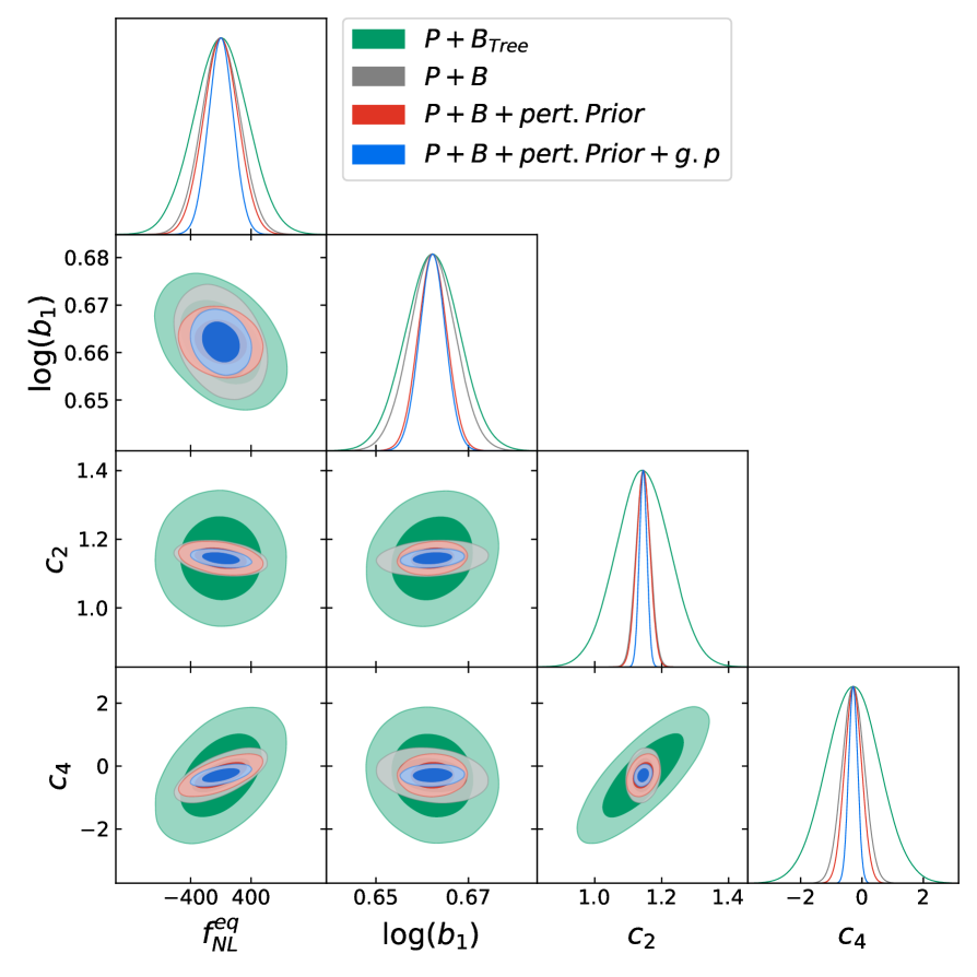
BOSS

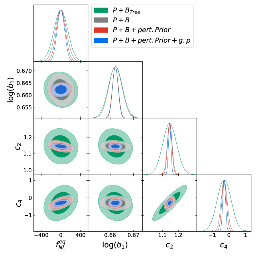
DESI

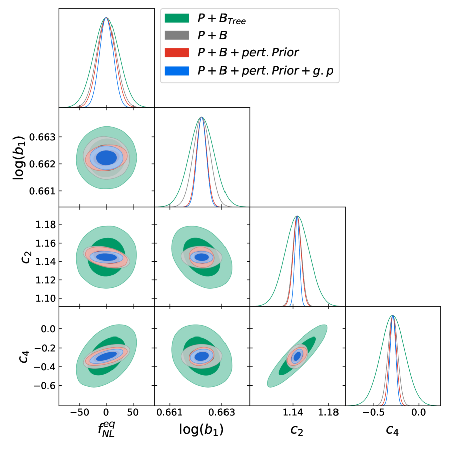
MegaMapper

BOSS: $\sigma(\cdot)$	$f_{\text{NL}}^{\text{loc.}}$	$f_{\text{NL}}^{\text{eq.}}$	$f_{\text{NL}}^{\text{orth.}}$	$\log(b_{1})$	$c_{2}$	$c_{4}$
$P$+$B_{\text{Tree}}$	37	357	142	0.006	0.081	0.88
$P$+$B$	23	253	67	0.005	0.021	0.36
$P$+$B$+p.p.	17	228	62	0.003	0.020	0.28
$P$+$B$+p.p.+g.p.	15	164	49	0.003	0.011	0.15

DESI: $\sigma(\cdot)$	$f_{\text{NL}}^{\text{loc.}}$	$f_{\text{NL}}^{\text{eq.}}$	$f_{\text{NL}}^{\text{orth.}}$	$\log(b_{1})$	$c_{2}$	$c_{4}$
$P$+$B_{\text{Tree}}$	3.61	142	71.5	0.003	0.04	0.4
$P$+$B$	3.46	114	30.2	0.003	0.02	0.2
$P$+$B$+p.p.	3.27	91.5	27.0	0.001	0.01	0.1
$P$+$B$+p.p.+g.p.	3.19	77.0	21.8	0.001	0.008	0.08

MMo: $\sigma(\cdot)$	$f_{\text{NL}}^{\text{loc.}}$	$f_{\text{NL}}^{\text{eq.}}$	$f_{\text{NL}}^{\text{orth.}}$	$\log(b_{1})$	$c_{2}$	$c_{4}$
$P$+$B_{\text{Tree}}$	0.29	23.4	8.7	0.0005	0.01	0.14
$P$+$B$	0.27	17.7	4.6	0.0003	0.005	0.05
$P+B$+p.p.	0.26	16.0	4.2	0.0002	0.005	0.04
$P$+$B$+p.p.+g.p.	0.26	12.6	3.4	0.0002	0.003	0.03

Figure 10: Triangle plots and errors from Fisher forecasts for BOSS (top left), DESI (top right), and MegaMapper (bottom left), for the equilateral type of non-Gaussianity, and leading bias parameters. We also show errors on other non-Gaussianity parameters in the tables. Each analysis was done with cosmological parameters fixed and each non-Gaussianity parameter was analyzed separately. We always include the power spectrum at one loop order with the addition of either the tree-level bispectrum the loop bispectrum or the loop bispectrum with a perturbativity prior (p.p.) also in combination with the “galaxy-formation prior” (g.p.). We use all power spectrum and bispectrum multipoles in each case and use the analytical covariance without cross-correlations.

BOSS

As shown in the table of Fig. 10, the one-loop bispectrum already significantly improves the constraints on non-Gaussianities by $\sim$ $30-50\%$ with respect to the tree-level analysis. Additionally including the perturbativity prior to the one-loop bispectrum yields a further $\sim$ 24% reduction in $\sigma$ for $f_{\text{NL}}^{\text{loc.}}$, and $\sim$ 10% reduction in $\sigma$ for $f_{\text{NL}}^{\text{eq.}}$ and $f_{\text{NL}}^{\text{orth.}}$. The “galaxy-formation prior” would further reduce the error by $\sim$ $20-30\%$ for $f_{\text{NL}}^{\text{eq.}}$ and $f_{\text{NL}}^{\text{orth.}}$, and 14% for $f_{\text{NL}}^{\text{loc.}}$. The addition of the loop breaks the degeneracy between $c_{2}$ and $c_{4}$ (), greatly improving constraints on both parameters, which translates to stronger constraints on $f_{\text{NL}}^{\text{eq.}}$. Furthermore, the inclusion of the perturbativity prior further breaks this degeneracy and improves upon the constraints on $b_{1}$, which leads to additional improvements on the $f_{\text{NL}}$ parameters.

DESI

As it was seen in BOSS, the inclusion of the loop bispectrum and perturbativity prior breaks the degeneracy between $c_{2}$ and $c_{4}$ and tightens the constraints on EFT parameters for DESI as well. However, the resulting effect on $f_{\text{NL}}$ parameters is different. Unlike BOSS, the inclusion of the one-loop bispectrum and perturbativity prior to DESI does not uniformly tighten all $f_{\text{NL}}$ errors. For one, most of the information to constrain $f_{\text{NL}}^{\text{loc.}}$ is contained in the power spectrum and the tree-level bispectrum. In contrast, the one-loop bispectrum does improve the constraint of $f_{\text{NL}}^{\text{eq.}}$ and $f_{\text{NL}}^{\text{orth.}}$ by 19% and 58% respectively. The perturbativity prior reduces these errors further by 20% and 11% and the future galaxy formation prior by another 16% and 19%.

MegaMapper

MegaMapper results are more similar to DESI than BOSS. $f_{\text{NL}}^{\text{loc.}}$ is mostly constrained through the power spectrum and does not improve much with the addition of the bispectrum loop or the perturbativity prior. Additionally, as was seen for DESI, the inclusion of the bispectrum loop leads to a more significant improvement in the constraint on $f_{\text{NL}}^{\text{orth.}}$ compared to $f_{\text{NL}}^{\text{eq.}}$, with 47% and 24% improvements respectively. To place these results into context, note that the tree level results we obtain are in agreement with those obtained in [102] . Note, however, the tree-level $k_{\text{max}}$ we estimate here is a bit lower, thus we predict slightly less optimistic constraints for the tree-level bispectrum, which makes the addition of the loop more important. The loop again breaks the degeneracy between $c_{2}$ and $c_{4}$, and the perturbativity prior enhances the constraints on $c_{2}$ in particular, thereby improving the constraints on $f_{\text{NL}}^{\text{eq.}}$ and $f_{\text{NL}}^{\text{orth.}}$ by $9\%$ and the “galaxy-formation prior” further reduces the errors by $21\%$ and $18\%$ respectively.

Appendix A Survey details and best-fits

Shown below are the exact parameter values that we use in the analyzes for each survey. Regarding cosmological parameters, for all surveys, we use the following best-fit as the reference cosmology  for the cosmological parameters (noted with a ${}^{\text{ref}}$).

$$h^{\text{ref}}=0.673\,,\qquad\ln(10^{10}A_{s})^{\text{ref}}=3.044\,,\qquad\Omega_{m}^{\text{ref}}=0.317\,,\qquad n_{s}^{\text{ref}}=0.965\,,$$ (A.1)

$$\Omega_{k}^{\text{ref}}=0\,,\qquad\omega_{b}^{\text{ref}}=0.022\,,\qquad{\sum_{i}m_{\nu_{i}}^{\text{ref}}=0.1}\,\text{eV}\,,\qquad f_{\text{NL}}^{\text{loc.},\text{ref}}=f_{\text{NL}}^{\text{eq.},\text{ref}}=f_{\text{NL}}^{\text{orth.},\text{ref}}=0\,.$$

Furthermore, in Tab. 4 we give the EFT parameter best-fit that we use, coming from [110]. Note, this is what we denote as $\vec{b}_{\text{BOSS}}$ (b1 - Bc14) and $\vec{\epsilon}_{\text{BOSS}}$ (Bd1 - Be12) in Sec. 2.3. Furthermore, we use the notation as in PyBird [18]. For a conversion to the notation of [110], see App. D.4 of [110]. The best-fit values of the 41 EFT parameters are given in Tab. 4.

Parameter	Value	Parameter	Value	Parameter	Value	Parameter	Value
b1	$1.94$	c2	$1.14$	b3	$-0.37$	c4	$-0.29$
b4	$0.13$	b6	$-0.35$	b7	$0.22$	b8	$-0.30$
b9	$0.015$	b10	$0.043$	b11	$0.036$	Bc1	$5.46$
Bc2	$-1.54$	Bc3	$1.31$	Bc4	$-0.48$	Bc5	$0.11$
Bc6	$0.87$	Bc7	$-0.46$	Bc8	$0.44$	Bc9	$-0.42$
Bc10	$-0.65$	Bc11	$-0.088$	Bc12	$-0.37$	Bc13	$-0.16$
Bc14	$-0.20$	Bd1	$5.4$	Bd2	$-0.72$	Bd3	$-0.43$
ce2	$0.55$	Be1	$1.69$	Be2	$0.91$	Be3	$0.074$
Be4	$-0.14$	Be5	$6.07$	Be6	$-0.093$	Be7	$-0.97$
Be8	$0.26$	Be9	$0.26$	Be10	$-0.15$	Be11	$0.43$
Be12	$-0.43$

Table 4: Best-fit EFT parameters.

Next, we show the survey specifications that were used in each survey. With the methods from Sec. 2, this builds the basis for the numerical values that we use in the forecasts.

BOSS

For the BOSS survey, we use the survey specifications as presented in [87, 123, 124, 125]. We display them in the same way they enter our formulas in Tab. 5.

$z$	$N_{g}$	$V[(h^{-1}{\rm Mpc})^{3}]$	$n_{b}[(h\,{\rm Mpc}^{-1})^{3}]$	$b_{1}$
0.05	7370	$2.55\times 10^{7}$	$2.9\times 10^{-4}$	1.48
0.15	47560	$1.64\times 10^{8}$	$2.9\times 10^{-4}$	1.56
0.25	120600	$4.02\times 10^{8}$	$3.0\times 10^{-4}$	1.65
0.35	214016	$7.04\times 10^{8}$	$3.0\times 10^{-4}$	1.73
0.45	287040	$1.04\times 10^{9}$	$2.8\times 10^{-4}$	1.83
0.55	445740	$1.38\times 10^{9}$	$3.2\times 10^{-4}$	1.92
0.65	206400	$1.72\times 10^{9}$	$1.2\times 10^{-4}$	2.02
0.75	20400	$2.04\times 10^{9}$	$1.0\times 10^{-5}$	2.12

Table 5: Survey details for each redshift bin for BOSS. We show the number of mapped galaxies $N_{g}$, the volume of the redshift bin $V$ as well as the number density $n_{b}$ and the linear bias $b_{1}$.

DESI

As mentioned in the main text, for DESI we focus on the largest sample which is the set of Emission Line Galaxies. The numerical values we use are calculated from table 2.3 in [88]. We present the specifications in Tab. 6.

$z$	$N_{g}$	$V[(h^{-1}{\rm Mpc})^{3}]$	$n_{b}[(h\,{\rm Mpc}^{-1})^{3}]$	$b_{1}$
0.65	432600	$2.63\times 10^{9}$	$1.64\times 10^{-4}$	1.18
0.75	$3.18\times 10^{6}$	$3.15\times 10^{9}$	$1.01\times 10^{-3}$	1.23
0.85	$2.70\times 10^{6}$	$3.65\times 10^{9}$	$7.38\times 10^{-4}$	1.29
0.95	$2.93\times 10^{6}$	$4.1\times 10^{9}$	$7.15\times 10^{-4}$	1.35
1.05	$2.02\times 10^{6}$	$4.52\times 10^{9}$	$4.46\times 10^{-4}$	1.41
1.15	$1.89\times 10^{6}$	$4.89\times 10^{9}$	$3.87\times 10^{-4}$	1.47
1.25	$1.87\times 10^{6}$	$5.22\times 10^{9}$	$3.59\times 10^{-4}$	1.53
1.35	732200	$5.5\times 10^{9}$	$1.33\times 10^{-4}$	1.59
1.45	652400	$5.75\times 10^{9}$	$1.13\times 10^{-4}$	1.65
1.55	460600	$5.97\times 10^{9}$	$7.71\times 10^{-5}$	1.72
1.65	176400	$6.15\times 10^{9}$	$2.87\times 10^{-5}$	1.78

Table 6: Survey details for each redshift bin for DESI. We show the number of mapped galaxies $N_{g}$, the volume of the redshift bin $V$ as well as the number density $n_{b}$ and the linear bias $b_{1}$.

MegaMapper

Finally, for MegaMapper, the specifications are still to be finalized given the early stage of the experiment compared to BOSS or DESI. We take the numerical values from [117, 89], where as mentioned in the main text there is an “idealized”, and a “fiducial” scenario. The specifications for the optimistic (or “idealized”) scenario are in Tab. 7. They are based on Tab. 1 of [117]. For the “fiducial” or what we call “pessimistic” scenario, we refer to table 2 in [117].

$z$	$N_{g}$	$V[(h^{-1}{\rm Mpc})^{3}]$	$n_{b}[(h\,{\rm Mpc}^{-1})^{3}]$	$b_{1}$
2	$6.75\times 10^{7}$	$2.70\times 10^{10}$	$2.5\times 10^{-3}$	2.5
2.5	$3.32\times 10^{7}$	$2.76\times 10^{10}$	$1.2\times 10^{-3}$	3.3
3	$1.63\times 10^{7}$	$2.72\times 10^{10}$	$6\times 10^{-4}$	4.1
3.5	$7.88\times 10^{6}$	$2.63\times 10^{10}$	$3\times 10^{-4}$	4.9
4	$3.76\times 10^{6}$	$2.51\times 10^{10}$	$1.5\times 10^{-4}$	5.8
4.5	$1.90\times 10^{6}$	$2.38\times 10^{10}$	$8\times 10^{-5}$	6.6
5	901730	$2.25\times 10^{10}$	$4\times 10^{-5}$	7.4

Table 7: Survey details for each redshift bin for MegaMapper (optimistic). We show the number of mapped galaxies $N_{g}$, the volume of the redshift bin $V$ as well as the number density $n_{b}$ and the linear bias $b_{1}$.

Appendix B Further analyses

Two further analyses, which to us do not carry the same significance as those presented in the main sections, are presented here for completeness. In Sec. B.1 we present results for the “pessimistic” scenario for MegaMapper as opposed to the “optimistic” scenario presented in Sec. 4.3. In Sec. B.2 we also present the impact of the perturbativity prior, as discussed in Sec. 5, on base cosmological parameters.

B.1 MegaMapper “pessimistic” results

The survey specifications for the “pessimistic” scenario given in Tab. 8 are determined with the methods described in Sec. 2.

MMp:	$z_{\text{eff}}$	$n_{b,\text{eff}}[(h\,{\rm Mpc}^{-1})^{3}]$	$b_{1}$	($k^{\text{Tree}}_{\rm max}$, $k^{1L}_{\rm max}$, $k_{\text{NL}}$) $[h\,{\rm Mpc}^{-1}]$	$N^{1L}_{\text{bins}}$	$N^{\text{Tree}}_{\Delta}$	$N^{1L}_{\Delta}$
Bin 1	2.1	8.8$\times 10^{-4}$	2.7	(0.12, 0.31, 2.2)	62	43	428
Bin 2	4.3	8.4$\times 10^{-5}$	4.0	(0.21, 0.57, 8.2)	114	150	2331

Table 8: MegaMapper “pessimistic” effective survey specifications, calculated according to the formulas in Sec. 2. $n_{b,\text{eff}}$ is the background galaxy number density entering the derivatives (not the covariance), $N_{\text{bins}}$ is the number of $k$-bins we consider for the power spectrum at 1-loop and $N_{\Delta}$ is the number of triangles we consider for the bispectrum at 1-loop.

To avoid redundancy with the discussion of the optimistic scenario, we here simply focus on base results for the pessimistic MegaMapper scenario. The discussion on fixing biases, shot noise and the inclusion of the perturbativity prior is comparable to the optimistic case. The only difference are the absolute values, while the relative gains are similar. We present results in Fig. 11, where we present the same base parameters as in the main section. Comparing to the figure and tables in Fig. 7 for almost all parameters we see only a $30-40\%$ difference compared to the optimistic case. The non-Gaussianity scenarios all differ by roughly $40-45\%$, independent on whether we use the tree-level bispectrum, the loop, or the perturbativity prior.

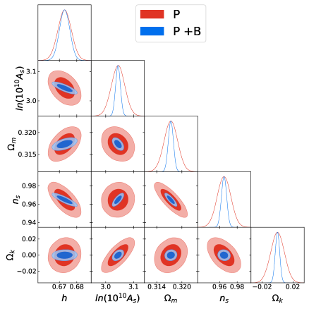
$\sigma(\cdot)$	$h$	$\ln(10^{10}A_{s})$	$\Omega_{m}$	$n_{s}$	$\Omega_{k}$
$P$	0.0039	0.024	0.0016	0.0078	0.009
$P$+$B$	0.003	0.009	0.0006	0.0030	0.003

$\sigma(\cdot)$	$h$	$\ln(10^{10}A_{s})$	$\Omega_{m}$	$\log m_{\nu}^{\text{tot.}}({}^{\sigma^{+}}_{\sigma^{-}})$
$P$	0.0032	0.031	0.0026	0.61(${}^{+0.08}_{-0.05}$)
$P$+$B$	0.0016	0.007	0.0007	0.14 (${}^{+0.015}_{-0.013}$)

$\sigma(\cdot)$	$f_{\text{NL}}^{\text{loc.}}$	$f_{\text{NL}}^{\text{eq.}}$	$f_{\text{NL}}^{\text{orth.}}$
$P$+$B_{\text{Tree}}$	0.45	40.8	18.1
$P$+$B$	0.44	32.9	8.5
$P$+$B$+p.p.	0.42	29.5	8.0
$P$+$B$+p.p.+g.p.	0.42	23.0	6.5

Figure 11: Triangle plots and errors from Fisher forecasts for MegaMapper (pessimistic) including the spectral tilt and spatial curvature (left) and massive neutrinos (right) and Non-Gaussianity (bottom). We use all power spectrum and bispectrum multipoles for the above results, and use the analytical covariance without cross-correlations. In the table we also report the upper and lower bounds of the $68\%$ confidence interval for the sum of massive neutrinos, i.e $\mathbb{P}\left[\left(\sum_{i}m_{\nu_{i}}-\sum_{i}m_{\nu_{i}}^{\text{ref}}\right)\in(\sigma^{-},\sigma^{+})\right]=0.68$. For non-Gaussianity, we also present results with only the inclusion of the tree-level bispectrum and with the inclusion of a perturbativity prior (p.p) and the “galaxy-formation prior” (g.p.).

B.2 Perturbativity prior effect on base cosmological parameters

We discuss here the effect of the perturbativity prior, also in combination with the galaxy formation prior, on base cosmological parameters. Results for all surveys are shown in Fig. 12. We see that the most notable effect is on $\ln(10^{10}A_{s})$, $n_{s}$ and $\Omega_{k}$, and a smaller effect on the other parameters. Furthermore, we found almost no improvement on constraints for neutrino masses.

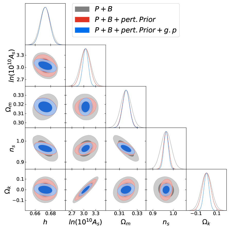
BOSS

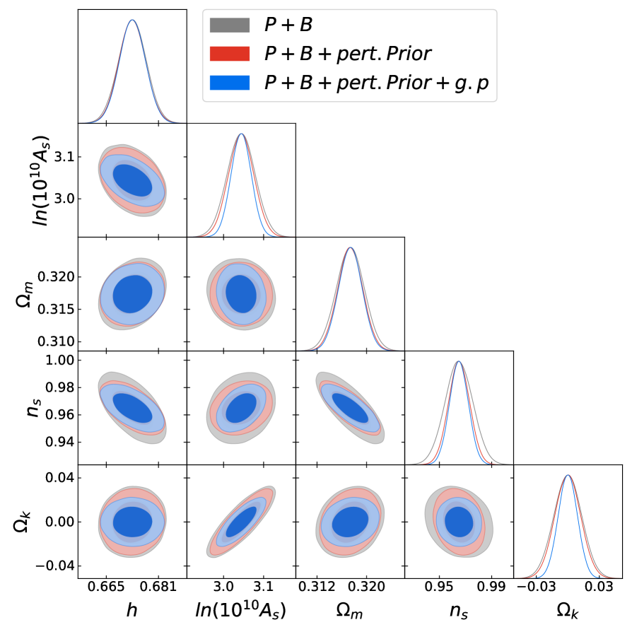
DESI

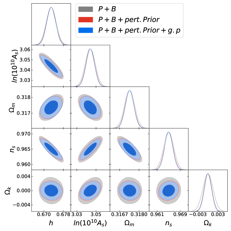
MegaMapper

BOSS:$\sigma(\cdot)$	$h$	$\ln(10^{10}A_{s})$	$\Omega_{m}$	$n_{s}$	$\Omega_{k}$
$P$+$B$	0.007	0.130	0.006	0.025	0.050
$P+B$+p.p.	0.006	0.110	0.004	0.013	0.041
$P$+$B$+p.p.+g.p.	0.006	0.069	0.004	0.011	0.025

DESI: $\sigma(\cdot)$	$h$	$\ln(10^{10}A_{s})$	$\Omega_{m}$	$n_{s}$	$\Omega_{k}$
$P$+$B$	0.004	0.035	0.002	0.011	0.013
$P+B$+p.p.	0.004	0.032	0.002	0.008	0.012
$P$+$B$+p.p.+g.p.	0.004	0.025	0.002	0.007	0.009

MMo: $\sigma(\cdot)$	$h$	$\ln(10^{10}A_{s})$	$\Omega_{m}$	$n_{s}$	$\Omega_{k}$
$P$+$B$	0.002	0.0052	0.0003	0.002	0.0015
$P+B$+p.p.	0.002	0.0046	0.0003	0.002	0.0012
$P$+$B$+p.p.+g.p.	0.002	0.0044	0.0003	0.001	0.0011

Figure 12: Triangle plots and errors from Fisher forecasts for BOSS (top left), DESI (top right), and MegaMapper (bottom left), for base cosmological parameters including the spectral tilt and spatial curvature. We always include the power spectrum at one loop order with the addition of either the loop bispectrum or the loop bispectrum with a perturbativity prior (p.p.) or also in combination with the “galaxy-formation prior” (g.p.). We use all power spectrum and bispectrum multipoles in each case and use the analytical covariance without cross-correlations.

References

- [1] D. Baumann, A. Nicolis, L. Senatore and M. Zaldarriaga, Cosmological Non-Linearities as an Effective Fluid, JCAP 1207 (2012) 051, [1004.2488].
- [2] J. J. M. Carrasco, M. P. Hertzberg and L. Senatore, The Effective Field Theory of Cosmological Large Scale Structures, JHEP 09 (2012) 082, [1206.2926].
- [3] G. D’Amico, J. Gleyzes, N. Kokron, D. Markovic, L. Senatore, P. Zhang et al., The Cosmological Analysis of the SDSS/BOSS data from the Effective Field Theory of Large-Scale Structure, JCAP 05 (2020) 005, [1909.05271].
- [4] M. M. Ivanov, M. Simonović and M. Zaldarriaga, Cosmological Parameters from the BOSS Galaxy Power Spectrum, JCAP 05 (2020) 042, [1909.05277].
- [5] T. Colas, G. D’amico, L. Senatore, P. Zhang and F. Beutler, Efficient Cosmological Analysis of the SDSS/BOSS data from the Effective Field Theory of Large-Scale Structure, JCAP 06 (2020) 001, [1909.07951].
- [6] Planck collaboration, N. Aghanim et al., Planck 2018 results. VI. Cosmological parameters, Astron. Astrophys. 641 (2020) A6, [1807.06209].
- [7] P. Zhang and Y. Cai, BOSS full-shape analysis from the EFTofLSS with exact time dependence, Journal of Cosmology and Astroparticle Physics 2022 (jan, 2022) 031.
- [8] P. Carrilho, C. Moretti and A. Pourtsidou, Cosmology with the EFTofLSS and BOSS: dark energy constraints and a note on priors, Journal of Cosmology and Astroparticle Physics 2023 (jan, 2023) 028.
- [9] P. Zhang, G. D’Amico, L. Senatore, C. Zhao and Y. Cai, BOSS Correlation Function Analysis from the Effective Field Theory of Large-Scale Structure, 2110.07539.
- [10] S.-F. Chen, Z. Vlah and M. White, A new analysis of the BOSS survey, including full-shape information and post-reconstruction BAO, 2110.05530.
- [11] T. Simon, P. Zhang and V. Poulin, Cosmological inference from the EFTofLSS: the eBOSS QSO full-shape analysis, 2210.14931.
- [12] O. H. E. Philcox and M. M. Ivanov, The BOSS DR12 Full-Shape Cosmology: CDM Constraints from the Large-Scale Galaxy Power Spectrum and Bispectrum Monopole, 2112.04515.
- [13] M. Tsedrik, C. Moretti, P. Carrilho, F. Rizzo and A. Pourtsidou, Interacting dark energy from the joint analysis of the power spectrum and bispectrum multipoles with the EFTofLSS, Monthly Notices of the Royal Astronomical Society 520 (jan, 2023) 2611–2632.
- [14] G. D’Amico, Y. Donath, M. Lewandowski, L. Senatore and P. Zhang, The boss bispectrum analysis at one loop from the effective field theory of large-scale structure, 2022.
- [15] O. H. Philcox, M. M. Ivanov, G. Cabass, M. Simonović, M. Zaldarriaga and T. Nishimichi, Cosmology with the redshift-space galaxy bispectrum monopole at one-loop order, Physical Review D 106 (aug, 2022) .
- [16] M. M. Ivanov, O. H. Philcox, G. Cabass, T. Nishimichi, M. Simonović and M. Zaldarriaga, Cosmology with the galaxy bispectrum multipoles: Optimal estimation and application to BOSS data, Physical Review D 107 (apr, 2023) .
- [17] O. H. E. Philcox, M. M. Ivanov, M. Simonović and M. Zaldarriaga, Combining Full-Shape and BAO Analyses of Galaxy Power Spectra: A 1.6\% CMB-independent constraint on H0, JCAP 05 (2020) 032, [2002.04035].
- [18] G. D’Amico, L. Senatore and P. Zhang, Limits on CDM from the EFTofLSS with the PyBird code, JCAP 01 (2021) 006, [2003.07956].
- [19] G. D’Amico, Y. Donath, L. Senatore and P. Zhang, Limits on Clustering and Smooth Quintessence from the EFTofLSS, 2012.07554.
- [20] A. G. Riess, S. Casertano, W. Yuan, L. M. Macri and D. Scolnic, Large Magellanic Cloud Cepheid Standards Provide a 1% Foundation for the Determination of the Hubble Constant and Stronger Evidence for Physics beyond CDM, Astrophys. J. 876 (2019) 85, [1903.07603].
- [21] W. L. Freedman et al., The Carnegie-Chicago Hubble Program. VIII. An Independent Determination of the Hubble Constant Based on the Tip of the Red Giant Branch, 1907.05922.
- [22] L. Verde, T. Treu and A. G. Riess, Tensions between the Early and the Late Universe, in Nature Astronomy 2019, 2019. 1907.10625. DOI.
- [23] G. D’Amico, L. Senatore, P. Zhang and H. Zheng, The Hubble Tension in Light of the Full-Shape Analysis of Large-Scale Structure Data, JCAP 05 (2021) 072, [2006.12420].
- [24] M. M. Ivanov, E. McDonough, J. C. Hill, M. Simonović, M. W. Toomey, S. Alexander et al., Constraining Early Dark Energy with Large-Scale Structure, Phys. Rev. D 102 (2020) 103502, [2006.11235].
- [25] F. Niedermann and M. S. Sloth, New Early Dark Energy is compatible with current LSS data, Phys. Rev. D 103 (2021) 103537, [2009.00006].
- [26] T. L. Smith, V. Poulin, J. L. Bernal, K. K. Boddy, M. Kamionkowski and R. Murgia, Early dark energy is not excluded by current large-scale structure data, Phys. Rev. D 103 (2021) 123542, [2009.10740].
- [27] T. Simon, P. Zhang, V. Poulin and T. L. Smith, Updated constraints from the effective field theory analysis of BOSS power spectrum on Early Dark Energy, 2208.05930.
- [28] G. D’Amico, M. Lewandowski, L. Senatore and P. Zhang, Limits on primordial non-Gaussianities from BOSS galaxy-clustering data, 2201.11518.
- [29] G. Cabass, M. M. Ivanov, O. H. E. Philcox, M. Simonović and M. Zaldarriaga, Constraints on Single-Field Inflation from the BOSS Galaxy Survey, Phys. Rev. Lett. 129 (2022) 021301, [2201.07238].
- [30] C. Moretti, M. Tsedrik, P. Carrilho and A. Pourtsidou, Modified gravity and massive neutrinos: constraints from the full shape analysis of BOSS galaxies and forecasts for Stage IV surveys, 2306.09275.
- [31] T. Simon, Constraining decaying dark matter with the effective field theory of large-scale structure, in 33rd Rencontres de Blois: Exploring the Dark Universe, 12, 2022. 2212.03004.
- [32] L. Piga, M. Marinucci, G. D’Amico, M. Pietroni, F. Vernizzi and B. S. Wright, Constraints on modified gravity from the BOSS galaxy survey, JCAP 04 (2023) 038, [2211.12523].
- [33] A. Chudaykin, K. Dolgikh and M. M. Ivanov, Constraints on the curvature of the Universe and dynamical dark energy from the Full-shape and BAO data, Phys. Rev. D 103 (2021) 023507, [2009.10106].
- [34] G. Cabass, M. M. Ivanov, O. H. E. Philcox, M. Simonović and M. Zaldarriaga, Constraints on multifield inflation from the BOSS galaxy survey, Phys. Rev. D 106 (2022) 043506, [2204.01781].
- [35] A. Semenaite, A. G. Sánchez, A. Pezzotta, J. Hou, A. Eggemeier, M. Crocce et al., Beyond – CDM constraints from the full shape clustering measurements from BOSS and eBOSS, Mon. Not. Roy. Astron. Soc. 521 (2023) 5013–5025, [2210.07304].
- [36] H. Rubira, A. Mazoun and M. Garny, Full-shape BOSS constraints on dark matter interacting with dark radiation and lifting the S8 tension, JCAP 01 (2023) 034, [2209.03974].
- [37] P. Carrilho, C. Moretti and A. Pourtsidou, Cosmology with the EFTofLSS and BOSS: dark energy constraints and a note on priors, JCAP 01 (2023) 028, [2207.14784].
- [38] T. Simon, G. Franco Abellán, P. Du, V. Poulin and Y. Tsai, Constraining decaying dark matter with BOSS data and the effective field theory of large-scale structures, Phys. Rev. D 106 (2022) 023516, [2203.07440].
- [39] R. A. Porto, L. Senatore and M. Zaldarriaga, The Lagrangian-space Effective Field Theory of Large Scale Structures, JCAP 1405 (2014) 022, [1311.2168].
- [40] J. J. M. Carrasco, S. Foreman, D. Green and L. Senatore, The 2-loop matter power spectrum and the IR-safe integrand, JCAP 1407 (2014) 056, [1304.4946].
- [41] J. J. M. Carrasco, S. Foreman, D. Green and L. Senatore, The Effective Field Theory of Large Scale Structures at Two Loops, JCAP 1407 (2014) 057, [1310.0464].
- [42] S. M. Carroll, S. Leichenauer and J. Pollack, Consistent effective theory of long-wavelength cosmological perturbations, Phys. Rev. D90 (2014) 023518, [1310.2920].
- [43] L. Senatore and M. Zaldarriaga, The IR-resummed Effective Field Theory of Large Scale Structures, JCAP 1502 (2015) 013, [1404.5954].
- [44] T. Baldauf, E. Schaan and M. Zaldarriaga, On the reach of perturbative methods for dark matter density fields, JCAP 1603 (2016) 007, [1507.02255].
- [45] S. Foreman, H. Perrier and L. Senatore, Precision Comparison of the Power Spectrum in the EFTofLSS with Simulations, JCAP 1605 (2016) 027, [1507.05326].
- [46] T. Baldauf, L. Mercolli and M. Zaldarriaga, Effective field theory of large scale structure at two loops: The apparent scale dependence of the speed of sound, Phys. Rev. D92 (2015) 123007, [1507.02256].
- [47] M. Cataneo, S. Foreman and L. Senatore, Efficient exploration of cosmology dependence in the EFT of LSS, 1606.03633.
- [48] M. Lewandowski and L. Senatore, IR-safe and UV-safe integrands in the EFTofLSS with exact time dependence, JCAP 1708 (2017) 037, [1701.07012].
- [49] T. Konstandin, R. A. Porto and H. Rubira, The Effective Field Theory of Large Scale Structure at Three Loops, 1906.00997.
- [50] E. Pajer and M. Zaldarriaga, On the Renormalization of the Effective Field Theory of Large Scale Structures, JCAP 1308 (2013) 037, [1301.7182].
- [51] A. A. Abolhasani, M. Mirbabayi and E. Pajer, Systematic Renormalization of the Effective Theory of Large Scale Structure, JCAP 1605 (2016) 063, [1509.07886].
- [52] L. Mercolli and E. Pajer, On the velocity in the Effective Field Theory of Large Scale Structures, JCAP 1403 (2014) 006, [1307.3220].
- [53] M. McQuinn and M. White, Cosmological perturbation theory in 1+1 dimensions, JCAP 1601 (2016) 043, [1502.07389].
- [54] L. Senatore, Bias in the Effective Field Theory of Large Scale Structures, JCAP 1511 (2015) 007, [1406.7843].
- [55] L. Senatore and M. Zaldarriaga, Redshift Space Distortions in the Effective Field Theory of Large Scale Structures, 1409.1225.
- [56] T. Baldauf, M. Mirbabayi, M. Simonovic and M. Zaldarriaga, Equivalence Principle and the Baryon Acoustic Peak, Phys. Rev. D92 (2015) 043514, [1504.04366].
- [57] L. Senatore and G. Trevisan, On the IR-Resummation in the EFTofLSS, JCAP 1805 (2018) 019, [1710.02178].
- [58] M. Lewandowski and L. Senatore, An analytic implementation of the IR-resummation for the BAO peak, 1810.11855.
- [59] D. Blas, M. Garny, M. M. Ivanov and S. Sibiryakov, Time-Sliced Perturbation Theory II: Baryon Acoustic Oscillations and Infrared Resummation, JCAP 1607 (2016) 028, [1605.02149].
- [60] M. Lewandowski, A. Perko and L. Senatore, Analytic Prediction of Baryonic Effects from the EFT of Large Scale Structures, JCAP 1505 (2015) 019, [1412.5049].
- [61] D. P. L. Bragança, M. Lewandowski, D. Sekera, L. Senatore and R. Sgier, Baryonic effects in the Effective Field Theory of Large-Scale Structure and an analytic recipe for lensing in CMB-S4, 2010.02929.
- [62] R. E. Angulo, S. Foreman, M. Schmittfull and L. Senatore, The One-Loop Matter Bispectrum in the Effective Field Theory of Large Scale Structures, JCAP 1510 (2015) 039, [1406.4143].
- [63] T. Baldauf, L. Mercolli, M. Mirbabayi and E. Pajer, The Bispectrum in the Effective Field Theory of Large Scale Structure, JCAP 1505 (2015) 007, [1406.4135].
- [64] D. Bertolini, K. Schutz, M. P. Solon and K. M. Zurek, The Trispectrum in the Effective Field Theory of Large Scale Structure, 1604.01770.
- [65] T. Baldauf, E. Schaan and M. Zaldarriaga, On the reach of perturbative descriptions for dark matter displacement fields, JCAP 1603 (2016) 017, [1505.07098].
- [66] S. Foreman and L. Senatore, The EFT of Large Scale Structures at All Redshifts: Analytical Predictions for Lensing, JCAP 1604 (2016) 033, [1503.01775].
- [67] M. Mirbabayi, F. Schmidt and M. Zaldarriaga, Biased Tracers and Time Evolution, JCAP 1507 (2015) 030, [1412.5169].
- [68] R. Angulo, M. Fasiello, L. Senatore and Z. Vlah, On the Statistics of Biased Tracers in the Effective Field Theory of Large Scale Structures, JCAP 1509 (2015) 029, [1503.08826].
- [69] T. Fujita, V. Mauerhofer, L. Senatore, Z. Vlah and R. Angulo, Very Massive Tracers and Higher Derivative Biases, 1609.00717.
- [70] A. Perko, L. Senatore, E. Jennings and R. H. Wechsler, Biased Tracers in Redshift Space in the EFT of Large-Scale Structure, 1610.09321.
- [71] E. O. Nadler, A. Perko and L. Senatore, On the Bispectra of Very Massive Tracers in the Effective Field Theory of Large-Scale Structure, JCAP 1802 (2018) 058, [1710.10308].
- [72] Y. Donath and L. Senatore, Biased Tracers in Redshift Space in the EFTofLSS with exact time dependence, JCAP 10 (2020) 039, [2005.04805].
- [73] P. McDonald and A. Roy, Clustering of dark matter tracers: generalizing bias for the coming era of precision LSS, JCAP 0908 (2009) 020, [0902.0991].
- [74] M. Lewandowski, L. Senatore, F. Prada, C. Zhao and C.-H. Chuang, EFT of large scale structures in redshift space, Phys. Rev. D97 (2018) 063526, [1512.06831].
- [75] L. Senatore and M. Zaldarriaga, The Effective Field Theory of Large-Scale Structure in the presence of Massive Neutrinos, 1707.04698.
- [76] R. de Belsunce and L. Senatore, Tree-Level Bispectrum in the Effective Field Theory of Large-Scale Structure extended to Massive Neutrinos, 1804.06849.
- [77] M. Lewandowski, A. Maleknejad and L. Senatore, An effective description of dark matter and dark energy in the mildly non-linear regime, JCAP 1705 (2017) 038, [1611.07966].
- [78] G. Cusin, M. Lewandowski and F. Vernizzi, Dark Energy and Modified Gravity in the Effective Field Theory of Large-Scale Structure, JCAP 1804 (2018) 005, [1712.02783].
- [79] B. Bose, K. Koyama, M. Lewandowski, F. Vernizzi and H. A. Winther, Towards Precision Constraints on Gravity with the Effective Field Theory of Large-Scale Structure, JCAP 1804 (2018) 063, [1802.01566].
- [80] V. Assassi, D. Baumann, E. Pajer, Y. Welling and D. van der Woude, Effective theory of large-scale structure with primordial non-Gaussianity, JCAP 1511 (2015) 024, [1505.06668].
- [81] V. Assassi, D. Baumann and F. Schmidt, Galaxy Bias and Primordial Non-Gaussianity, JCAP 1512 (2015) 043, [1510.03723].
- [82] D. Bertolini, K. Schutz, M. P. Solon, J. R. Walsh and K. M. Zurek, Non-Gaussian Covariance of the Matter Power Spectrum in the Effective Field Theory of Large Scale Structure, 1512.07630.
- [83] D. Bertolini and M. P. Solon, Principal Shapes and Squeezed Limits in the Effective Field Theory of Large Scale Structure, 1608.01310.
- [84] M. Simonovic, T. Baldauf, M. Zaldarriaga, J. J. Carrasco and J. A. Kollmeier, Cosmological perturbation theory using the FFTLog: formalism and connection to QFT loop integrals, JCAP 1804 (2018) 030, [1708.08130].
- [85] T. Nishimichi, G. D’Amico, M. M. Ivanov, L. Senatore, M. Simonović, M. Takada et al., Blinded challenge for precision cosmology with large-scale structure: results from effective field theory for the redshift-space galaxy power spectrum, Phys. Rev. D 102 (2020) 123541, [2003.08277].
- [86] S.-F. Chen, Z. Vlah, E. Castorina and M. White, Redshift-Space Distortions in Lagrangian Perturbation Theory, JCAP 03 (2021) 100, [2012.04636].
- [87] BOSS collaboration, S. Alam et al., The clustering of galaxies in the completed SDSS-III Baryon Oscillation Spectroscopic Survey: cosmological analysis of the DR12 galaxy sample, Mon. Not. Roy. Astron. Soc. 470 (2017) 2617–2652, [1607.03155].
- [88] DESI collaboration, A. Aghamousa et al., The DESI Experiment Part I: Science,Targeting, and Survey Design, 1611.00036.
- [89] D. J. Schlegel et al., The MegaMapper: A Stage-5 Spectroscopic Instrument Concept for the Study of Inflation and Dark Energy, 2209.04322.
- [90] D. J. H. Chung, M. Münchmeyer and S. C. Tadepalli, Search for Isocurvature with Large-scale Structure: A Forecast for Euclid and MegaMapper using EFTofLSS, 2306.09456.
- [91] T. Kajita, Nobel Lecture: Discovery of atmospheric neutrino oscillations, Rev. Mod. Phys. 88 (2016) 030501.
- [92] R. Bousso, D. Harlow and L. Senatore, Inflation after False Vacuum Decay: observational Prospects after Planck, Phys. Rev. D 91 (2015) 083527, [1309.4060].
- [93] M. Kleban and M. Schillo, Spatial Curvature Falsifies Eternal Inflation, JCAP 06 (2012) 029, [1202.5037].
- [94] D. Babich, P. Creminelli and M. Zaldarriaga, The Shape of non-Gaussianities, JCAP 08 (2004) 009, [astro-ph/0405356].
- [95] P. Creminelli, A. Nicolis, L. Senatore, M. Tegmark and M. Zaldarriaga, Limits on non-gaussianities from wmap data, JCAP 0605 (2006) 004, [astro-ph/0509029].
- [96] L. Senatore, K. M. Smith and M. Zaldarriaga, Non-Gaussianities in Single Field Inflation and their Optimal Limits from the WMAP 5-year Data, JCAP 1001 (2010) 028, [0905.3746].
- [97] C. Cheung, P. Creminelli, A. L. Fitzpatrick, J. Kaplan and L. Senatore, The Effective Field Theory of Inflation, JHEP 03 (2008) 014, [0709.0293].
- [98] F. Bernardeau and J.-P. Uzan, NonGaussianity in multifield inflation, Phys. Rev. D 66 (2002) 103506, [hep-ph/0207295].
- [99] D. H. Lyth, C. Ungarelli and D. Wands, The Primordial density perturbation in the curvaton scenario, Phys. Rev. D 67 (2003) 023503, [astro-ph/0208055].
- [100] M. Zaldarriaga, Non-Gaussianities in models with a varying inflaton decay rate, Phys. Rev. D 69 (2004) 043508, [astro-ph/0306006].
- [101] L. Senatore and M. Zaldarriaga, The Effective Field Theory of Multifield Inflation, JHEP 04 (2012) 024, [1009.2093].
- [102] G. Cabass, M. M. Ivanov, O. H. E. Philcox, M. Simonovic and M. Zaldarriaga, Constraining single-field inflation with MegaMapper, Phys. Lett. B 841 (2023) 137912, [2211.14899].
- [103] R. Flauger, M. Mirbabayi, L. Senatore and E. Silverstein, Productive Interactions: heavy particles and non-Gaussianity, JCAP 10 (2017) 058, [1606.00513].
- [104] C. Anastasiou, D. P. L. Bragança, L. Senatore and H. Zheng, Efficiently evaluating loop integrals in the EFTofLSS using QFT integrals with massive propagators, 2212.07421.
- [105] Planck collaboration, Y. Akrami et al., Planck 2018 results. IX. Constraints on primordial non-Gaussianity, Astron. Astrophys. 641 (2020) A9, [1905.05697].
- [106] M. Tegmark, Measuring cosmological parameters with galaxy surveys, Phys. Rev. Lett. 79 (1997) 3806–3809, [astro-ph/9706198].
- [107] N. Agarwal, V. Desjacques, D. Jeong and F. Schmidt, Information content in the redshift-space galaxy power spectrum and bispectrum, JCAP 03 (2021) 021, [2007.04340].
- [108] V. Yankelevich and C. Porciani, Cosmological information in the redshift-space bispectrum, Mon. Not. Roy. Astron. Soc. 483 (2019) 2078–2099, [1807.07076].
- [109] D. Baumann, D. Green and B. Wallisch, Searching for light relics with large-scale structure, JCAP 08 (2018) 029, [1712.08067].
- [110] G. D’Amico, Y. Donath, M. Lewandowski, L. Senatore and P. Zhang, The BOSS bispectrum analysis at one loop from the Effective Field Theory of Large-Scale Structure, 2206.08327.
- [111] G. D’Amico, Y. Donath, M. Lewandowski, L. Senatore and P. Zhang, The one-loop bispectrum of galaxies in redshift space from the Effective Field Theory of Large-Scale Structure, 2211.17130.
- [112] H. A. Feldman, N. Kaiser and J. A. Peacock, Power spectrum analysis of three-dimensional redshift surveys, Astrophys. J. 426 (1994) 23–37, [astro-ph/9304022].
- [113] R. Scoccimarro, S. Colombi, J. N. Fry, J. A. Frieman, E. Hivon and A. Melott, Nonlinear evolution of the bispectrum of cosmological perturbations, Astrophys. J. 496 (1998) 586, [astro-ph/9704075].
- [114] K. C. Chan and L. Blot, Assessment of the Information Content of the Power Spectrum and Bispectrum, Phys. Rev. D 96 (2017) 023528, [1610.06585].
- [115] E. Sefusatti, M. Crocce, S. Pueblas and R. Scoccimarro, Cosmology and the Bispectrum, Phys. Rev. D 74 (2006) 023522, [astro-ph/0604505].
- [116] V. Desjacques, D. Jeong and F. Schmidt, Large-Scale Galaxy Bias, Phys. Rept. 733 (2018) 1–193, [1611.09787].
- [117] S. Ferraro et al., Inflation and Dark Energy from Spectroscopy at , Bull. Am. Astron. Soc. 51 (2019) 72, [1903.09208].
- [118] N. Kokron, J. DeRose, S.-F. Chen, M. White and R. H. Wechsler, Priors on red galaxy stochasticity from hybrid effective field theory, Mon. Not. Roy. Astron. Soc. 514 (2022) 2198–2213, [2112.00012].
- [119] C. Alcock and B. Paczynski, An evolution free test for non-zero cosmological constant, Nature 281 (1979) 358–359.
- [120] T. Baldauf, U. Seljak and L. Senatore, Primordial non-Gaussianity in the Bispectrum of the Halo Density Field, JCAP 04 (2011) 006, [1011.1513].
- [121] Y. Donath and L. Senatore, Exact Trispectrum covariances and Fisher matrices, in progress.
- [122] T. Steele and T. Baldauf, Precise Calibration of the One-Loop Trispectrum in the Effective Field Theory of Large Scale Structure, Phys. Rev. D 103 (2021) 103518, [2101.10289].
- [123] B. Reid et al., SDSS-III Baryon Oscillation Spectroscopic Survey Data Release 12: galaxy target selection and large scale structure catalogues, Mon. Not. Roy. Astron. Soc. 455 (2016) 1553–1573, [1509.06529].
- [124] BOSS collaboration, F. Beutler et al., The clustering of galaxies in the completed SDSS-III Baryon Oscillation Spectroscopic Survey: Anisotropic galaxy clustering in Fourier-space, Mon. Not. Roy. Astron. Soc. 466 (2017) 2242–2260, [1607.03150].
- [125] A. Font-Ribera, P. McDonald, N. Mostek, B. A. Reid, H.-J. Seo and A. Slosar, DESI and other dark energy experiments in the era of neutrino mass measurements, JCAP 05 (2014) 023, [1308.4164].