Model-Driven Sensing-Node Selection and Power Allocation for Tracking Maneuvering Targets in Perceptive Mobile Networks

Lei Xie, , Shenghui Song, , and Yonina C. Eldar,  L. Xie and S. Song are with Department of Electronic and Computer Engineering, the Hong Kong University of Science and Technology, Hong Kong. e-mail: ({{\{eelxie, eeshsong}}\}@ust.hk). Y. C. Eldar is with the Faculty of Mathematics and Computer Science, Weizmann Institute of Science, Rehovot 7610001, Israel (e-mail: yonina.eldar@weizmann.ac.il).
Abstract

Maneuvering target tracking will be an important service of future wireless networks to assist innovative applications such as intelligent transportation. However, tracking maneuvering targets by cellular networks faces many challenges. For example, the dense network and high-speed targets make the selection of the sensing nodes (SNs), e.g., base stations, and the associated power allocation very difficult, given the stringent latency requirement of sensing applications. Existing methods have demonstrated engaging tracking performance, but with very high computational complexity. In this paper, we propose a model-driven deep learning approach for SN selection to meet the latency requirement. To this end, we first propose an iterative SN selection method by jointly exploiting the majorization-minimization (MM) framework and the alternating direction method of multipliers (ADMM). Then, we unfold the iterative algorithm as a deep neural network (DNN) and prove its convergence. The proposed model-driven method has a low computational complexity, because the number of layers is less than the number of iterations required by the original algorithm, and each layer only involves simple matrix-vector additions/multiplications. Finally, we propose an efficient power allocation method based on fixed point (FP) water filling (WF) and solve the joint SN selection and power allocation problem under the alternative optimization framework. Simulation results show that the proposed method achieves better performance than the conventional optimization-based methods with much lower computational complexity.

Index Terms:
Maneuvering target tracking, perceptive mobile network, model-driven deep learning, sensing node selection, power allocation.

I Introduction

Innovative applications such as intelligent transportation systems require high-precision sensing capabilities, which are unavailable from current cellular networks. To this end, the recently proposed integrated sensing and communication (ISAC) paradigm offers a promising way to share spectrum, hardware, and software between sensing and communication [1, 2]. Perceptive mobile network (PMN) was proposed as a special type of ISAC system that adds high-precision sensing capability to the cellular networks [3, 4, 5, 6]. There are many favorable properties of cellular networks that can facilitate sensing. For instance, the large number of sensing nodes (SNs) in PMNs enables collaborative sensing, where multiple perspectives from different SNs are exploited to sense the same target. The SNs can be base station (BS) [1], road side units [2], remote radio unit [3], or target monitoring terminal [4].

However, tracking maneuvering targets by PMNs faces many challenges. For example, due to the dense cellular network, selecting a proper set of SNs to track a moving target can be very difficult, because the handover from one group of SNs to another faces very stringent latency requirements. There have been engaging results on SN selection and power allocation for tracking maneuvering targets [7, 8, 9, 10, 11, 12, 13, 14, 15]. The authors of [7] proposed two SN selection methods in wireless networks to minimize the posterior Cramér-Rao lower bound (PCRLB) and maximize the mutual information between the target location and the measurements of the selected SNs, respectively. In [8], a cooperative game theoretic approach was utilized to allocate power for tracking targets in a radar network. The authors of [9] proposed two strategies for resource allocation with given SNs, where one maximizes the tracking accuracy with limited power budgets, and the other minimizes the power consumption with required tracking performance.

To achieve better performance, the joint SN selection and power allocation schemes were also considered [14, 15]. In [14], a distributed multi-target tracking method was proposed for the networked multiple-input multiple-output (MIMO) radar system, where an alternative optimization (AO)-based method was utilized to solve the bi-variable optimization problem. The boolean constraint on the SN selection vector is one of the most critical challenges for the joint SN selection and power allocation problem. To handle this issue, a typical method is to relax the boolean constraint to allow continuous and sparse variables [16, 17, 15]. In [14, 15], the relaxed SN selection was formulated as a semi-definite programming (SDP) problem and solved by the CVX toolbox [18]. Unfortunately, the complexity of the existing methods increases exponentially with the number of SNs, which may violate the stringent latency requirement of sensing applications when a large number of SNs exist.

To this end, model-driven deep learning (DL) offers a promising solution. By unfolding an iterative algorithm as a neural network where each iteration is implemented by one layer with learnable parameters, model-driven methods have the potential to offer better performance with reduced computational complexity. Some research efforts have been made to utilize model-driven deep neural networks (DNNs) to find sparse solutions for better performance and lower computational costs. In [19], an unfolded vector-approximate message passing network with random initialization was proposed to learn a denoiser identical to the statistically matched one. The authors of [20] unfolded the iterative algorithm, used to solve a problem with l0subscript𝑙0l_{0} sparse regularization, to be a feed-forward neural network for faster inference and better scalability. In [21], a generalized DNN was proposed to learn a sparse solution by unfolding the alternating direction method of multipliers (ADMM) with better accuracy and lower computational cost. The authors of [22] designed an ADMM-Net for interference removal in radar imaging, which exhibited much lower imaging error and computational cost than ADMM and CVX. However, the inverse of high-dimensional matrices are involved in the existing ADMM-based unfolding methods, which causes high storage and computational cost.

In this paper, to meet the stringent latency requirement of sensing applications, we propose a model-driven method for SN selection to track multiple maneuvering targets. For that purpose, we first derive an iterative algorithm for SN selection, leveraging the majorization-minimization (MM) framework and ADMM. Then, the MM-ADMM algorithm is unfolded into a DNN where the technical challenges lie in the large number of learnable parameters and the uncertain convergence property. To this end, we design a new model-driven DNN with an additional module to exploit the first- and second-order momentum, and refer to it as deep alternating network (DAN), which has fewer learnable parameters than the directly-unfolded MM-ADMM. The convergence proof of the proposed DAN is also given. The computational complexity of DAN is low, because the number of layers is less than the number of iterations required by the original algorithm, and each layer of DAN only involves simple matrix-vector additions/multiplications without high-dimensional matrix inverse. Finally, we propose a fixed-point (FP) water-filling (WF)-based method for power allocation, which is derived based on the Lagrange multiplier method. The joint SN selection and power allocation problem is solved by combining the proposed DAN and FP-WF algorithms under the AO framework. Experiment results show that the proposed method can achieve better performance than the optimization-based methods with remarkably lower computational costs.

The contributions of this paper are summarized as follows:

  1. 1.

    We propose an iterative method based on MM and ADMM for SN selection. In particular, we exploit the MM approach to handle the non-convexity of the penalized cost functions. For each iteration of ADMM, we derive explicit expressions for the solution to the constrained optimization problem by exploiting the KKT conditions, which facilitate the development of the model-driven method.

  2. 2.

    We design a new model-driven DNN, named DAN, by adding an additional module to the directly-unfolded MM-ADMM method, which exploits the momentum for accelerating the convergence. Moreover, we provide the convergence proof for DAN, which achieves a similar SN selection performance as the exhaustive searching method with significantly lower computational cost.

  3. 3.

    Inspired by the classic WF-based power allocation strategies, we propose an iterative FP-WF power allocation method. Specifically, in each water-filling step, the water level is obtained by solving an FP equation. This approach not only reduces the computational complexity, but also provides an interesting physical insight: the power allocation strategy depends on the ratio between the Fisher information of the predictions and the measurements.

The remainder of this paper is organized as follows. Section II introduces the system model and formulates the problem. Section III derives the joint SN selection and power allocation algorithm. Section IV provides the simulation results to validate the advantage of the proposed model-driven method. Section V concludes this paper.

II System Model and Problem Formulation

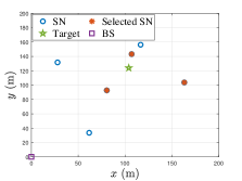
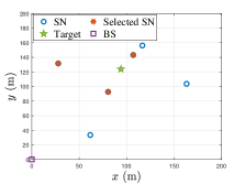
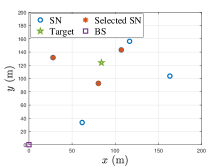
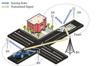
In Fig. 1, we show a PMN consisting of one BS serving as the sensing signal transmitter and N𝑁N SNs serving as the receivers for the echoes, which can be BSs or other types of SNs [1, 2, 3, 4]. In each tracking frame, the BS will transmit sensing signals to the predicted positions of multiple targets, and the selected SNs will collaboratively estimate the location and velocity of the targets (motion state). The estimation results will be utilized to predict the motion state in the next tracking frame111The tracked targets are initialized and the number of the targets is known in advance. This assumption can be realized by communication or some available detection approaches, e.g., radio access technology [23], PDA [24] or multi-frame detection [25] before target tracking. The targets are widely separated and each of them moves independently in the monitoring area [13].. In this paper, the SN selection and power allocation will be formulated as an optimization problem to minimize the PCRLB for the estimation error of the target motion state. To this end, we first introduce the target motion model and the signal model, which are the foundation for deriving the PCRLB.
Refer to caption
Figure 1: Illustration of the system.

II-A Target Motion Model

The target motion model describes the motion behavior of the targets and affects the Fisher information of the prediction. Assume that the target motion follows a near constant velocity model and the transition matrix 𝐆𝐆\mathbf{G} is given by [12, 11, 13, 15]

𝐆=𝐈2[1ΔT01]𝐆tensor-productsubscript𝐈2delimited-[]matrix1Δ𝑇01\begin{split}\mathbf{G}=\mathbf{I}_{2}\otimes\left[\begin{matrix}1&\Delta T\\ 0&1\\ \end{matrix}\right]\end{split} (1)

where 𝐈2subscript𝐈2\mathbf{I}_{2} denotes the 2×2222\times 2 identity matrix, tensor-product\otimes represents the Kronecker product, and ΔTΔ𝑇\Delta T denotes the time between two adjacent tracking frames. In the k𝑘kth tracking frame, there are Q𝑄Q point-like targets, where the q𝑞qth target is located at 𝐫q(k)=(rx,q(k),ry,q(k))superscriptsubscript𝐫𝑞𝑘superscriptsubscript𝑟𝑥𝑞𝑘superscriptsubscript𝑟𝑦𝑞𝑘\mathbf{r}_{q}^{(k)}=(r_{x,q}^{(k)},r_{y,q}^{(k)}) with a velocity 𝐯q(k)=(vx,q(k),vy,q(k))superscriptsubscript𝐯𝑞𝑘superscriptsubscript𝑣𝑥𝑞𝑘superscriptsubscript𝑣𝑦𝑞𝑘\mathbf{v}_{q}^{(k)}=(v_{x,q}^{(k)},v_{y,q}^{(k)}). The target motion state is updated by 𝐱q(k)=𝐆𝐱q(k1)+𝐳q(k1)superscriptsubscript𝐱𝑞𝑘superscriptsubscript𝐆𝐱𝑞𝑘1superscriptsubscript𝐳𝑞𝑘1\mathbf{x}_{q}^{(k)}=\mathbf{G}\mathbf{x}_{q}^{(k-1)}+\mathbf{z}_{q}^{(k-1)}, where 𝐱q(k)=[rx,q(k),vx,q(k),ry,q(k),vy,q(k)]Tsuperscriptsubscript𝐱𝑞𝑘superscriptsuperscriptsubscript𝑟𝑥𝑞𝑘superscriptsubscript𝑣𝑥𝑞𝑘superscriptsubscript𝑟𝑦𝑞𝑘superscriptsubscript𝑣𝑦𝑞𝑘T\mathbf{x}_{q}^{(k)}=[r_{x,q}^{(k)},v_{x,q}^{(k)},r_{y,q}^{(k)},v_{y,q}^{(k)}]^{\mathrm{T}} includes the parameters to be estimated. Here, 𝐳q(k1)superscriptsubscript𝐳𝑞𝑘1\mathbf{z}_{q}^{(k-1)} denotes the state noise, which is assumed to be a zero-mean Gaussian vector with covariance matrix [12, 11]

𝐐=qs𝐈2[13(ΔT)312(ΔT)212(ΔT)2ΔT]𝐐tensor-productsubscript𝑞𝑠subscript𝐈2delimited-[]matrix13superscriptΔ𝑇312superscriptΔ𝑇212superscriptΔ𝑇2Δ𝑇\begin{split}\mathbf{Q}=q_{s}\mathbf{I}_{2}\otimes\left[\begin{matrix}\frac{1}{3}(\Delta T)^{3}&\frac{1}{2}(\Delta T)^{2}\\ \frac{1}{2}(\Delta T)^{2}&\Delta T\\ \end{matrix}\right]\end{split} (2)

where qssubscript𝑞𝑠q_{s} is the intensity of the process noise.

II-B Signal Model

In the k𝑘kth tracking frame, the BS will transmit the sensing signal 𝐬(k)(t)superscript𝐬𝑘𝑡\mathbf{s}^{(k)}(t) to the targets, and the echoes will be captured by the selected SNs for sensing purposes. The location of the BS and the n𝑛nth SN is given by 𝐫BSsubscript𝐫𝐵𝑆\mathbf{r}_{BS} and 𝐫nsubscript𝐫𝑛\mathbf{r}_{n}, respectively. Given the motion state, we can determine the measurements, i.e., the angle of arrival (AOA), the time delay, and the Doppler frequency of the q𝑞q-th target with respect to the n𝑛n-th SN as

θq,n(k)=arccos𝐞nT(𝐫q(k)𝐫n)𝐫q(k)𝐫n,superscriptsubscript𝜃𝑞𝑛𝑘superscriptsubscript𝐞𝑛Tsuperscriptsubscript𝐫𝑞𝑘subscript𝐫𝑛normsuperscriptsubscript𝐫𝑞𝑘subscript𝐫𝑛\displaystyle\theta_{q,n}^{(k)}=\arccos\frac{\mathbf{e}_{n}^{\mathrm{T}}(\mathbf{r}_{q}^{(k)}-\mathbf{r}_{n})}{\|\mathbf{r}_{q}^{(k)}-\mathbf{r}_{n}\|}, (3)
τq,n(k)=1c(𝐫n𝐫q(k)+𝐫BS𝐫q(k)),superscriptsubscript𝜏𝑞𝑛𝑘1𝑐normsubscript𝐫𝑛superscriptsubscript𝐫𝑞𝑘normsubscript𝐫𝐵𝑆superscriptsubscript𝐫𝑞𝑘\displaystyle\tau_{q,n}^{(k)}=\frac{1}{c}\left(\|\mathbf{r}_{n}-\mathbf{r}_{q}^{(k)}\|+\|\mathbf{r}_{BS}-\mathbf{r}_{q}^{(k)}\|\right), (4)
μq,n(k)=𝐯qT(𝐫q(k)𝐫n)λ𝐫q(k)𝐫n+𝐯qT(𝐫q(k)𝐫BS)λ𝐫q(k)𝐫BS,superscriptsubscript𝜇𝑞𝑛𝑘superscriptsubscript𝐯𝑞Tsuperscriptsubscript𝐫𝑞𝑘subscript𝐫𝑛𝜆normsuperscriptsubscript𝐫𝑞𝑘subscript𝐫𝑛superscriptsubscript𝐯𝑞Tsuperscriptsubscript𝐫𝑞𝑘subscript𝐫𝐵𝑆𝜆normsuperscriptsubscript𝐫𝑞𝑘subscript𝐫𝐵𝑆\displaystyle\mu_{q,n}^{(k)}=\frac{\mathbf{v}_{q}^{\mathrm{T}}(\mathbf{r}_{q}^{(k)}-\mathbf{r}_{n})}{\lambda\|\mathbf{r}_{q}^{(k)}-\mathbf{r}_{n}\|}+\frac{\mathbf{v}_{q}^{\mathrm{T}}(\mathbf{r}_{q}^{(k)}-\mathbf{r}_{BS})}{\lambda\|\mathbf{r}_{q}^{(k)}-\mathbf{r}_{BS}\|}, (5)

where 𝐞nsubscript𝐞𝑛\mathbf{e}_{n} represents the unit vector parallel to the line formed by all antennas of the uniform linear array, c𝑐c is the speed of light, λ𝜆\lambda is the wavelength, and ||||||\cdot|| denotes the l2subscript𝑙2l_{2} norm.

Define the power allocation vector 𝐩(k)=[p1(k),,pQ(k)]Q×1superscript𝐩𝑘superscriptsubscript𝑝1𝑘superscriptsubscript𝑝𝑄𝑘superscript𝑄1\mathbf{p}^{(k)}=[p_{1}^{(k)},\cdots,p_{Q}^{(k)}]\in\mathbb{R}^{Q\times 1}, where pq(k)superscriptsubscript𝑝𝑞𝑘p_{q}^{(k)} denotes the power allocated to the q𝑞qth target. The baseband echo of the q𝑞qth target received by the n𝑛nth SN is given by

𝐲q,n(k)(t)=pq(k)βq,n(k)ej2πμq,n(k)t𝐛q,n(k)𝐚q,kH𝐬(k)(tτq,n(k))+𝐧n(k)(t),superscriptsubscript𝐲𝑞𝑛𝑘𝑡superscriptsubscript𝑝𝑞𝑘superscriptsubscript𝛽𝑞𝑛𝑘superscript𝑒𝑗2𝜋superscriptsubscript𝜇𝑞𝑛𝑘𝑡superscriptsubscript𝐛𝑞𝑛𝑘superscriptsubscript𝐚𝑞𝑘Hsuperscript𝐬𝑘𝑡superscriptsubscript𝜏𝑞𝑛𝑘superscriptsubscript𝐧𝑛𝑘𝑡\begin{split}\mathbf{y}_{q,n}^{(k)}(t)&=\sqrt{p_{q}^{(k)}}\beta_{q,n}^{(k)}e^{j2\pi\mu_{q,n}^{(k)}t}\mathbf{b}_{q,n}^{(k)}\mathbf{a}_{q,k}^{\mathrm{H}}\mathbf{s}^{(k)}(t-\tau_{q,n}^{(k)})\\ &\quad+\mathbf{n}_{n}^{(k)}(t),\end{split} (6)

where 𝐧n(k)(t)superscriptsubscript𝐧𝑛𝑘𝑡\mathbf{n}_{n}^{(k)}(t) denotes the complex additive white Gaussian noise with zero mean and variance σ2superscript𝜎2\sigma^{2}. The transmit and receive steering vectors are given by 𝐛q,n(k)=𝐛(θq,n(k))superscriptsubscript𝐛𝑞𝑛𝑘𝐛superscriptsubscript𝜃𝑞𝑛𝑘\mathbf{b}_{q,n}^{(k)}=\mathbf{b}(\theta_{q,n}^{(k)}) and 𝐚q,k=𝐚(ψq(k))subscript𝐚𝑞𝑘𝐚superscriptsubscript𝜓𝑞𝑘\mathbf{a}_{q,k}=\mathbf{a}(\psi_{q}^{(k)}), respectively, where ψq(k)superscriptsubscript𝜓𝑞𝑘\psi_{q}^{(k)} represents the angle of departure (AOD) of the q𝑞qth target from the BS. βq,n(k)superscriptsubscript𝛽𝑞𝑛𝑘\beta_{q,n}^{(k)} represents the complex gain of the BS-target-SN (q𝑞qth target and n𝑛nth SN) path, which accounts for the array gain, the propagation loss and the target radar cross section (RCS) [26].

Following [12, 11, 13, 14, 15], the local estimation error is modeled as a zero-mean Gaussian vector with the covariance matrix

𝚺q,n(k)=diag[σθq,n(k)2,στq,n(k)2,σμq,n(k)2],superscriptsubscript𝚺𝑞𝑛𝑘diagsuperscriptsubscript𝜎superscriptsubscript𝜃𝑞𝑛𝑘2superscriptsubscript𝜎superscriptsubscript𝜏𝑞𝑛𝑘2superscriptsubscript𝜎superscriptsubscript𝜇𝑞𝑛𝑘2\begin{split}\mathbf{\Sigma}_{q,n}^{(k)}=\mathrm{diag}\left[\sigma_{\theta_{q,n}^{(k)}}^{2},\sigma_{\tau_{q,n}^{(k)}}^{2},\sigma_{\mu_{q,n}^{(k)}}^{2}\right],\end{split} (7)

where σθq,n(k)2superscriptsubscript𝜎superscriptsubscript𝜃𝑞𝑛𝑘2\sigma_{\theta_{q,n}^{(k)}}^{2}, στq,n(k)2superscriptsubscript𝜎superscriptsubscript𝜏𝑞𝑛𝑘2\sigma_{\tau_{q,n}^{(k)}}^{2}, and σμq,n(k)2superscriptsubscript𝜎superscriptsubscript𝜇𝑞𝑛𝑘2\sigma_{\mu_{q,n}^{(k)}}^{2} denote the CRLBs for the estimation of the direction, range, and Doppler shift, respectively. The local estimation error affects the Fisher information of measurement, which will be utilized to derive the PCRLB in the next section.

II-C Posterior Cramér-Rao Lower Bound

Based on the above-mentioned target motion model and signal model, we will derive the PCRLB, which gives the lower bound of the estimation error for the target motion state. Define 𝐔(k)=[𝐮1(k),,𝐮Q(k)]NBS×Qsuperscript𝐔𝑘superscriptsubscript𝐮1𝑘superscriptsubscript𝐮𝑄𝑘superscriptsubscript𝑁𝐵𝑆𝑄\mathbf{U}^{(k)}=[\mathbf{u}_{1}^{(k)},\cdots,\mathbf{u}_{Q}^{(k)}]\in\mathbb{R}^{N_{BS}\times Q} as the SN selection matrix, whose (n,q)𝑛𝑞(n,q)th entry uq,n(k)superscriptsubscript𝑢𝑞𝑛𝑘u_{q,n}^{(k)} is 1 if the q𝑞qth target is associated with the n𝑛nth SN. The Fisher information matrix (FIM) for the q𝑞qth target is given by [27]

𝐉q(k)(pq(k),𝐮q(k))=𝐉P,q(k)+𝐉Z,q(k),superscriptsubscript𝐉𝑞𝑘superscriptsubscript𝑝𝑞𝑘superscriptsubscript𝐮𝑞𝑘superscriptsubscript𝐉𝑃𝑞𝑘superscriptsubscript𝐉𝑍𝑞𝑘\mathbf{J}_{q}^{(k)}(p_{q}^{(k)},\mathbf{u}_{q}^{(k)})=\mathbf{J}_{P,q}^{(k)}+\mathbf{J}_{Z,q}^{(k)}, (8)

where 𝐉P,q(k)superscriptsubscript𝐉𝑃𝑞𝑘\mathbf{J}_{P,q}^{(k)} and 𝐉Z,q(k)superscriptsubscript𝐉𝑍𝑞𝑘\mathbf{J}_{Z,q}^{(k)} denote the prior and data information matrix, respectively. In particular, the prior information matrix is given by

𝐉P,q(k)=(𝐐+𝐆(𝐉q(k1))1𝐆H)1.superscriptsubscript𝐉𝑃𝑞𝑘superscript𝐐𝐆superscriptsuperscriptsubscript𝐉𝑞𝑘11superscript𝐆H1\mathbf{J}_{P,q}^{(k)}=\left(\mathbf{Q}+\mathbf{G}(\mathbf{J}_{q}^{(k-1)})^{-1}\mathbf{G}^{\mathrm{H}}\right)^{-1}. (9)

The data information matrix 𝐉Z,q(k)superscriptsubscript𝐉𝑍𝑞𝑘\mathbf{J}_{Z,q}^{(k)} is given by

𝐉Z,q(k)=n=1Nuq,n(k)(𝐇q,n(k))T(𝚺q,n(k))1𝐇q,n(k),superscriptsubscript𝐉𝑍𝑞𝑘superscriptsubscript𝑛1𝑁superscriptsubscript𝑢𝑞𝑛𝑘superscriptsuperscriptsubscript𝐇𝑞𝑛𝑘Tsuperscriptsuperscriptsubscript𝚺𝑞𝑛𝑘1superscriptsubscript𝐇𝑞𝑛𝑘\mathbf{J}_{Z,q}^{(k)}=\sum_{n=1}^{N}u_{q,n}^{(k)}(\mathbf{H}_{q,n}^{(k)})^{\mathrm{T}}(\mathbf{\Sigma}_{q,n}^{(k)})^{-1}\mathbf{H}_{q,n}^{(k)}, (10)

where

𝐇q,n(k)=𝐠n(k)𝐱q(k)|𝐱q(k)=𝐱^q(k|k1),superscriptsubscript𝐇𝑞𝑛𝑘evaluated-atsuperscriptsubscript𝐠𝑛𝑘superscriptsubscript𝐱𝑞𝑘superscriptsubscript𝐱𝑞𝑘superscriptsubscript^𝐱𝑞conditional𝑘𝑘1\mathbf{H}_{q,n}^{(k)}=\frac{\partial\mathbf{g}_{n}^{(k)}}{\partial\mathbf{x}_{q}^{(k)}}\bigg{|}_{\mathbf{x}_{q}^{(k)}=\hat{\mathbf{x}}_{q}^{(k|k-1)}}, (11)

with 𝐠n(k)𝐱q(k)superscriptsubscript𝐠𝑛𝑘superscriptsubscript𝐱𝑞𝑘\frac{\partial\mathbf{g}_{n}^{(k)}}{\partial\mathbf{x}_{q}^{(k)}} denoting the derivative of the measurements 𝐠n(k)=[θq,n(k)(𝐱q(k)),τq,n(k)(𝐱q(k)),μq,n(k)(𝐱q(k))]Tsuperscriptsubscript𝐠𝑛𝑘superscriptsuperscriptsubscript𝜃𝑞𝑛𝑘superscriptsubscript𝐱𝑞𝑘superscriptsubscript𝜏𝑞𝑛𝑘superscriptsubscript𝐱𝑞𝑘superscriptsubscript𝜇𝑞𝑛𝑘superscriptsubscript𝐱𝑞𝑘T\mathbf{g}_{n}^{(k)}=[\theta_{q,n}^{(k)}(\mathbf{x}_{q}^{(k)}),\tau_{q,n}^{(k)}(\mathbf{x}_{q}^{(k)}),\mu_{q,n}^{(k)}(\mathbf{x}_{q}^{(k)})]^{\mathrm{T}} with respect to the motion state 𝐱q(k)superscriptsubscript𝐱𝑞𝑘\mathbf{x}_{q}^{(k)}. The predicted motion state of the q𝑞qth target in the k𝑘kth frame is updated by 𝐱^q(k|k1)=𝐆𝐱^q(k1),superscriptsubscript^𝐱𝑞conditional𝑘𝑘1𝐆superscriptsubscript^𝐱𝑞𝑘1\hat{\mathbf{x}}_{q}^{(k|k-1)}=\mathbf{G}\hat{\mathbf{x}}_{q}^{(k-1)}, where 𝐱^q(k1)superscriptsubscript^𝐱𝑞𝑘1\hat{\mathbf{x}}_{q}^{(k-1)} represents the estimated motion state of the q𝑞qth target in the (k1)𝑘1(k-1)th frame. Note that 𝚺q,n(k)superscriptsubscript𝚺𝑞𝑛𝑘\mathbf{\Sigma}_{q,n}^{(k)} is inversely proportional to the SNR at the SN [12, 11, 13, 14, 15]. Thus, we can rewrite the measurement covariance in (7) as

𝚺q,n(k)=(pq(k))1𝚺¯q,n(k),superscriptsubscript𝚺𝑞𝑛𝑘superscriptsuperscriptsubscript𝑝𝑞𝑘1superscriptsubscript¯𝚺𝑞𝑛𝑘\mathbf{\Sigma}_{q,n}^{(k)}=(p_{q}^{(k)})^{-1}\bar{\mathbf{\Sigma}}_{q,n}^{(k)}, (12)

where 𝚺¯q,n(k)superscriptsubscript¯𝚺𝑞𝑛𝑘\bar{\mathbf{\Sigma}}_{q,n}^{(k)} contains the part of 𝚺q,n(k)superscriptsubscript𝚺𝑞𝑛𝑘\mathbf{\Sigma}_{q,n}^{(k)} that is independent of pq(k)superscriptsubscript𝑝𝑞𝑘p_{q}^{(k)}. Then, we have 𝐉Z,q(k)=pq(k)n=1Nuq,n(k)𝐌¯q,n(k)superscriptsubscript𝐉𝑍𝑞𝑘superscriptsubscript𝑝𝑞𝑘superscriptsubscript𝑛1𝑁superscriptsubscript𝑢𝑞𝑛𝑘superscriptsubscript¯𝐌𝑞𝑛𝑘\mathbf{J}_{Z,q}^{(k)}=p_{q}^{(k)}\sum_{n=1}^{N}u_{q,n}^{(k)}\overline{\mathbf{M}}_{q,n}^{(k)}, where 𝐌¯q,n(k)=(𝐇q,n(k))T(𝚺¯q,n(k))1𝐇q,n(k)superscriptsubscript¯𝐌𝑞𝑛𝑘superscriptsuperscriptsubscript𝐇𝑞𝑛𝑘Tsuperscriptsuperscriptsubscript¯𝚺𝑞𝑛𝑘1superscriptsubscript𝐇𝑞𝑛𝑘\overline{\mathbf{M}}_{q,n}^{(k)}=(\mathbf{H}_{q,n}^{(k)})^{\mathrm{T}}(\bar{\mathbf{\Sigma}}_{q,n}^{(k)})^{-1}\mathbf{H}_{q,n}^{(k)}. Note that 𝐌q,n(k)=pq(k)𝐌¯q,n(k)superscriptsubscript𝐌𝑞𝑛𝑘superscriptsubscript𝑝𝑞𝑘superscriptsubscript¯𝐌𝑞𝑛𝑘\mathbf{M}_{q,n}^{(k)}=p_{q}^{(k)}\overline{\mathbf{M}}_{q,n}^{(k)} denotes the measurement information for the q𝑞qth target at the n𝑛nth SN. The inverse of the derived FIM yields the PCRLB matrix, i.e., [12, 11, 13, 14, 15]

𝐂q(pq(k),𝐮q(k))=(𝐉q(k)(pq(k),𝐮q(k)))1.subscript𝐂𝑞superscriptsubscript𝑝𝑞𝑘superscriptsubscript𝐮𝑞𝑘superscriptsuperscriptsubscript𝐉𝑞𝑘superscriptsubscript𝑝𝑞𝑘superscriptsubscript𝐮𝑞𝑘1\mathbf{C}_{q}(p_{q}^{(k)},\mathbf{u}_{q}^{(k)})=\left(\mathbf{J}_{q}^{(k)}(p_{q}^{(k)},\mathbf{u}_{q}^{(k)})\right)^{-1}. (13)

The diagonal elements of 𝐂q(pq(k),𝐮q(k))subscript𝐂𝑞superscriptsubscript𝑝𝑞𝑘superscriptsubscript𝐮𝑞𝑘\mathbf{C}_{q}(p_{q}^{(k)},\mathbf{u}_{q}^{(k)}) provide a lower bound on the variances of the estimation error of an unbiased estimator for the target motion state, i.e.,

𝔼((𝐱^q(k)𝐱q(k))(𝐱^q(k)𝐱q(k))H)𝐂q(pq(k),𝐮q(k)),succeeds-or-equals𝔼superscriptsubscript^𝐱𝑞𝑘superscriptsubscript𝐱𝑞𝑘superscriptsuperscriptsubscript^𝐱𝑞𝑘superscriptsubscript𝐱𝑞𝑘Hsubscript𝐂𝑞superscriptsubscript𝑝𝑞𝑘superscriptsubscript𝐮𝑞𝑘\mathbb{E}\left((\hat{\mathbf{x}}_{q}^{(k)}-\mathbf{x}_{q}^{(k)})(\hat{\mathbf{x}}_{q}^{(k)}-\mathbf{x}_{q}^{(k)})^{\mathrm{H}}\right)\succeq\mathbf{C}_{q}(p_{q}^{(k)},\mathbf{u}_{q}^{(k)}), (14)

where 𝐀𝐁succeeds-or-equals𝐀𝐁\mathbf{A}\succeq\mathbf{B} indicates 𝐀𝐁𝐀𝐁\mathbf{A}-\mathbf{B} is a positive-semidefinite matrix. Some functions of the diagonal elements of the PCRLB matrix, e.g., the trace [12] and the determinant [28, 29], have been used as the performance metric for target sensing and tracking.

II-D Problem Formulation

We want to minimize the PCRLB through SN selection and power allocation. In the k𝑘kth frame, the problem is modeled as

min𝐩(k),𝐔(k)subscriptsuperscript𝐩𝑘superscript𝐔𝑘\displaystyle\min_{\mathbf{p}^{(k)},\mathbf{U}^{(k)}}\; q=1Qlogdet𝐂q(pq(k),𝐮q(k))superscriptsubscript𝑞1𝑄subscript𝐂𝑞superscriptsubscript𝑝𝑞𝑘superscriptsubscript𝐮𝑞𝑘\displaystyle\sum_{q=1}^{Q}\log\det\mathbf{C}_{q}(p_{q}^{(k)},\mathbf{u}_{q}^{(k)})
s.t. q=1Qpq(k)PT,superscriptsubscript𝑞1𝑄superscriptsubscript𝑝𝑞𝑘subscript𝑃𝑇\displaystyle\sum_{q=1}^{Q}p_{q}^{(k)}\leq P_{T}, (15a)
pq(k)Pmin,superscriptsubscript𝑝𝑞𝑘subscript𝑃\displaystyle p_{q}^{(k)}\geq P_{\min}, (15b)
𝟏T𝐮q(k)Nmax,q=1,2,,Q,formulae-sequencesuperscript1Tsuperscriptsubscript𝐮𝑞𝑘subscript𝑁𝑞12𝑄\displaystyle\mathbf{1}^{\mathrm{T}}\mathbf{u}_{q}^{(k)}\leq N_{\max},q=1,2,\cdots,Q, (15c)
𝐔(k){0,1}N×Q,superscript𝐔𝑘superscript01𝑁𝑄\displaystyle\mathbf{U}^{(k)}\in\{0,1\}^{N\times Q}, (15d)

where constraint (15a) limits the total transmit power. Constraint (15b) indicates the minimum power allocated to each target, constraint (15c) limits the maximum number of SNs to track one target [30], and (15d) gives the binary constraint on 𝐮q(k)superscriptsubscript𝐮𝑞𝑘\mathbf{u}_{q}^{(k)}. The main reasons to select logdet(𝐂q)subscript𝐂𝑞\log\det(\mathbf{C}_{q}) as the performance metric include: 1) the determinant of 𝐂qsubscript𝐂𝑞\mathbf{C}_{q} is proportional to the volume of the minimum achievable covariance ellipsoid, which is widely used as an important metric for parameter estimation [28, 29]; and 2) if the determinant is directly used, the original problem (15) is not convex, but the monotonic logarithmic transformations can render this problem convex.

III Model-Driven Sensing Node Selection and Power Allocation Scheme

Note that the problem in (15) has two variables. To handle this issue, we propose to update the variables alternatively based on the AO theory. With a given feasible starting point {𝐩(k,0),{𝐮q(k,0)}q=1Q}superscript𝐩𝑘0superscriptsubscriptsuperscriptsubscript𝐮𝑞𝑘0𝑞1𝑄\left\{{\mathbf{p}}^{(k,0)},\{{\mathbf{u}}_{q}^{(k,0)}\}_{q=1}^{Q}\right\}, we iteratively perform the following two operations:

1) updating {𝐮q(k,j+1)}q=1Qsuperscriptsubscriptsuperscriptsubscript𝐮𝑞𝑘𝑗1𝑞1𝑄\{{\mathbf{u}}_{q}^{(k,j+1)}\}_{q=1}^{Q} with fixed 𝐩(k,j)superscript𝐩𝑘𝑗{\mathbf{p}}^{(k,j)} via

𝐮q(k,j+1)=argmin𝐮q(k)logdet𝐂q(pq(k,j),𝐮q(k)),superscriptsubscript𝐮𝑞𝑘𝑗1subscriptsuperscriptsubscript𝐮𝑞𝑘subscript𝐂𝑞superscriptsubscript𝑝𝑞𝑘𝑗superscriptsubscript𝐮𝑞𝑘\begin{split}\mathbf{u}_{q}^{(k,j+1)}=&\arg\min_{\mathbf{u}_{q}^{(k)}}\log\det\mathbf{C}_{q}(p_{q}^{(k,j)},\mathbf{u}_{q}^{(k)}),\end{split} (16)

2) updating 𝐩(k,j+1)superscript𝐩𝑘𝑗1{\mathbf{p}}^{(k,j+1)} with fixed {𝐮q(k,j+1)}q=1Qsuperscriptsubscriptsuperscriptsubscript𝐮𝑞𝑘𝑗1𝑞1𝑄\{{\mathbf{u}}_{q}^{(k,j+1)}\}_{q=1}^{Q} via

𝐩(k,j+1)=argmin𝐩(k)q=1Qlogdet𝐂q(pq(k),𝐮q(k,j+1)),superscript𝐩𝑘𝑗1subscriptsuperscript𝐩𝑘superscriptsubscript𝑞1𝑄subscript𝐂𝑞superscriptsubscript𝑝𝑞𝑘superscriptsubscript𝐮𝑞𝑘𝑗1\mathbf{p}^{(k,j+1)}=\arg\min_{\mathbf{p}^{(k)}}\sum_{q=1}^{Q}\log\det\mathbf{C}_{q}(p_{q}^{(k)},\mathbf{u}_{q}^{(k,j+1)}), (17)

which decouple the SN selection and power allocation problem.

In the following, we will first derive an iterative method for SN selection by jointly exploiting the MM framework and ADMM. To further reduce the computational complexity, we will develop a model-driven approach to solve (16). Finally, we will propose an FP-based WF method to solve (17), which has much lower complexity but offers comparable performance as the traditional CVX-based method.

III-A MM-ADMM based Sensing Node Selection

Given 𝐩(k,j)superscript𝐩𝑘𝑗\mathbf{p}^{(k,j)}, the problem in (16) can be formulated as

min𝐮q(k)u(𝐮q(k))s.t.𝟏T𝐮q(k)Nmax,𝐮q(k){0,1}N×1,formulae-sequencesubscriptsuperscriptsubscript𝐮𝑞𝑘subscript𝑢superscriptsubscript𝐮𝑞𝑘s.t.superscript1Tsuperscriptsubscript𝐮𝑞𝑘subscript𝑁superscriptsubscript𝐮𝑞𝑘superscript01𝑁1\begin{split}\min_{\mathbf{u}_{q}^{(k)}}\;&\mathcal{F}_{u}(\mathbf{u}_{q}^{(k)})\\ \text{s.t.}\;&\mathbf{1}^{\mathrm{T}}\mathbf{u}_{q}^{(k)}\leq N_{\max},\;\mathbf{u}_{q}^{(k)}\in\{0,1\}^{N\times 1},\end{split} (18)

where u(𝐮q(k))=logdet𝐂q(𝐮q(k)|pq(k,j))subscript𝑢superscriptsubscript𝐮𝑞𝑘subscript𝐂𝑞conditionalsuperscriptsubscript𝐮𝑞𝑘superscriptsubscript𝑝𝑞𝑘𝑗\mathcal{F}_{u}(\mathbf{u}_{q}^{(k)})=\log\det\mathbf{C}_{q}(\mathbf{u}_{q}^{(k)}|p_{q}^{(k,j)}). In order to enforce a binary solution and simplify the problem, we introduce a l0subscript𝑙0l_{0} pseudo-norm penalty to the objective function and relax the binary constraint [31]. Then, the problem in (18) is relaxed as

min𝐮q(k)u(𝐮q(k))+ρq𝐮q(k)0s.t.𝟏T𝐮q(k)Nmax, 0𝐮q(k)𝟏,formulae-sequencesubscriptsuperscriptsubscript𝐮𝑞𝑘subscript𝑢superscriptsubscript𝐮𝑞𝑘subscript𝜌𝑞subscriptdelimited-∥∥superscriptsubscript𝐮𝑞𝑘0s.t.superscript1Tsuperscriptsubscript𝐮𝑞𝑘subscript𝑁 0superscriptsubscript𝐮𝑞𝑘1\begin{split}\min_{\mathbf{u}_{q}^{(k)}}\;&\mathcal{F}_{u}(\mathbf{u}_{q}^{(k)})+\rho_{q}\|\mathbf{u}_{q}^{(k)}\|_{0}\\ \text{s.t.}\;&\mathbf{1}^{\mathrm{T}}\mathbf{u}_{q}^{(k)}\leq N_{\max},\;\mathbf{0}\leq\mathbf{u}_{q}^{(k)}\leq\mathbf{1},\end{split} (19)

where 0\|\cdot\|_{0} denotes the l0subscript𝑙0l_{0} pseudo-norm. In general, a larger ρqsubscript𝜌𝑞\rho_{q} leads to a sparser 𝐮q(k)superscriptsubscript𝐮𝑞𝑘\mathbf{u}_{q}^{(k)}. Due to the non-convex, non-continuous, and combinatorial nature of the l0subscript𝑙0l_{0} pseudo-norm, the problem (19) is NP-hard. To simplify the notation, we omit the index q𝑞q hereafter unless doing so creates confusion.

Inspired by [32], we approximate the l0subscript𝑙0l_{0} pseudo-norm by a function 𝒫γ(𝐮(k))=n=1N(1eγun(k))subscript𝒫𝛾superscript𝐮𝑘superscriptsubscript𝑛1𝑁1superscript𝑒𝛾superscriptsubscript𝑢𝑛𝑘\mathcal{P}_{\gamma}(\mathbf{u}^{(k)})=\sum_{n=1}^{N}(1-e^{-\gamma u_{n}^{(k)}}), where γ𝛾\gamma is a sufficiently large constant. 𝒫γ(𝐮(k))subscript𝒫𝛾superscript𝐮𝑘\mathcal{P}_{\gamma}(\mathbf{u}^{(k)}) is utilized due to several favorable properties: 1) it is asymptotically equivalent to 𝐮(k)0subscriptnormsuperscript𝐮𝑘0\|\mathbf{u}^{(k)}\|_{0}, i.e., limγ𝒫γ(𝐮(k))=n=1N(1δ(un(k)))=𝐮(k)0subscript𝛾subscript𝒫𝛾superscript𝐮𝑘superscriptsubscript𝑛1𝑁1𝛿superscriptsubscript𝑢𝑛𝑘subscriptnormsuperscript𝐮𝑘0\lim_{\gamma\to\infty}\mathcal{P}_{\gamma}(\mathbf{u}^{(k)})=\sum_{n=1}^{N}(1-\delta(u_{n}^{(k)}))=\|\mathbf{u}^{(k)}\|_{0}; 2) it is continuous, concave, and non-decreasing in the feasible set; and 3) it is differentiable and its gradient is easy to obtain.

III-A1 MM framework for solving (19)

The problem in (19) can be approximated by

min𝐮(k)𝒮uu(𝐮(k))+ρ𝒫γ(𝐮(k))subscriptsuperscript𝐮𝑘subscript𝒮𝑢subscript𝑢superscript𝐮𝑘𝜌subscript𝒫𝛾superscript𝐮𝑘\begin{split}\min_{\mathbf{u}^{(k)}\in\mathcal{S}_{u}}\;&\mathcal{F}_{u}(\mathbf{u}^{(k)})+\rho\mathcal{P}_{\gamma}(\mathbf{u}^{(k)})\end{split} (20)

where 𝒮u={𝐮(k)|𝟏T𝐮(k)=Nmax,𝟎𝐮(k)𝟏}subscript𝒮𝑢conditional-setsuperscript𝐮𝑘formulae-sequencesuperscript1Tsuperscript𝐮𝑘subscript𝑁0superscript𝐮𝑘1\mathcal{S}_{u}=\{\mathbf{u}^{(k)}|\mathbf{1}^{\mathrm{T}}\mathbf{u}^{(k)}=N_{\max},\mathbf{0}\leq\mathbf{u}^{(k)}\leq\mathbf{1}\}. Though 𝒫γ(𝐮(k))subscript𝒫𝛾superscript𝐮𝑘\mathcal{P}_{\gamma}(\mathbf{u}^{(k)}) is continuous w.r.t. 𝐮(k)superscript𝐮𝑘\mathbf{u}^{(k)}, the problem in (20) is still hard to solve, due to the complicated form of u(𝐮(k))subscript𝑢superscript𝐮𝑘\mathcal{F}_{u}(\mathbf{u}^{(k)}) w.r.t. 𝐮(k)superscript𝐮𝑘\mathbf{u}^{(k)}. To handle this difficulty, we propose to utilize the MM framework [33], based on which (20) can be solved in an iterative process. At each iteration, the MM framework updates the optimization variable by minimizing a tight upperbound of the function, which is known as the surrogate function. Then, The next question is how to construct a surrogate function for the objective function in (20).

Since 𝒫γ(𝐮(k))subscript𝒫𝛾superscript𝐮𝑘\mathcal{P}_{\gamma}(\mathbf{u}^{(k)}) is differentiable and concave with respect to 𝐮(k)superscript𝐮𝑘\mathbf{u}^{(k)}, it is upperbounded by its first-order Taylor expansion, i.e.,

𝒫γ(𝐮(k))𝒫~γ(𝐮(k)|𝐮(k,l))𝒫γ(𝐮(k,l))+(𝐝γ(k,l))T(𝐮(k)𝐮(k,l)),subscript𝒫𝛾superscript𝐮𝑘subscript~𝒫𝛾conditionalsuperscript𝐮𝑘superscript𝐮𝑘𝑙subscript𝒫𝛾superscript𝐮𝑘𝑙superscriptsuperscriptsubscript𝐝𝛾𝑘𝑙Tsuperscript𝐮𝑘superscript𝐮𝑘𝑙\begin{split}&\mathcal{P}_{\gamma}(\mathbf{u}^{(k)})\leq\widetilde{\mathcal{P}}_{\gamma}(\mathbf{u}^{(k)}|\mathbf{u}^{(k,l)})\\ &\triangleq\mathcal{P}_{\gamma}(\mathbf{u}^{(k,l)})+(\mathbf{d}_{\gamma}^{(k,l)})^{\mathrm{T}}(\mathbf{u}^{(k)}-\mathbf{u}^{(k,l)}),\\ \end{split} (21)

where 𝐮(k,l)superscript𝐮𝑘𝑙\mathbf{u}^{(k,l)} denotes the optimized result at the l𝑙lth iteration, 𝐝γ(k,l)=γ[eγu1(k,l),eγu2(k,l),,eγuN(k,l)]Tsuperscriptsubscript𝐝𝛾𝑘𝑙𝛾superscriptsuperscript𝑒𝛾superscriptsubscript𝑢1𝑘𝑙superscript𝑒𝛾superscriptsubscript𝑢2𝑘𝑙superscript𝑒𝛾superscriptsubscript𝑢𝑁𝑘𝑙T\mathbf{d}_{\gamma}^{(k,l)}=\gamma[e^{-\gamma u_{1}^{(k,l)}},e^{-\gamma u_{2}^{(k,l)}},\cdots,e^{-\gamma u_{N}^{(k,l)}}]^{\mathrm{T}} represents the gradient of 𝒫γ(𝐮(k))subscript𝒫𝛾superscript𝐮𝑘\mathcal{P}_{\gamma}(\mathbf{u}^{(k)}), and un(k,l)superscriptsubscript𝑢𝑛𝑘𝑙u_{n}^{(k,l)} denotes the n𝑛nth entry of 𝐮(k,l)superscript𝐮𝑘𝑙\mathbf{u}^{(k,l)}.

An appropriate upperbound of u(𝐮(k))subscript𝑢superscript𝐮𝑘\mathcal{F}_{u}(\mathbf{u}^{(k)}) can be obtained by

𝒢~1(𝐮(k)|𝐮(k,l))u(𝐮(k,l))+𝐝uT(𝐮(k,l))(𝐮(k)𝐮(k,l))subscript~𝒢1conditionalsuperscript𝐮𝑘superscript𝐮𝑘𝑙subscript𝑢superscript𝐮𝑘𝑙superscriptsubscript𝐝𝑢Tsuperscript𝐮𝑘𝑙superscript𝐮𝑘superscript𝐮𝑘𝑙\displaystyle\widetilde{\mathcal{G}}_{1}(\mathbf{u}^{(k)}|\mathbf{u}^{(k,l)})\triangleq\mathcal{F}_{u}(\mathbf{u}^{(k,l)})+\mathbf{d}_{u}^{\mathrm{T}}(\mathbf{u}^{(k,l)})(\mathbf{u}^{(k)}-\mathbf{u}^{(k,l)})
+12(𝐮(k)𝐮(k,l))T𝐓(k,l)(𝐮(k)𝐮(k,l)),12superscriptsuperscript𝐮𝑘superscript𝐮𝑘𝑙Tsuperscript𝐓𝑘𝑙superscript𝐮𝑘superscript𝐮𝑘𝑙\displaystyle\quad+\frac{1}{2}(\mathbf{u}^{(k)}-\mathbf{u}^{(k,l)})^{\mathrm{T}}\mathbf{T}^{(k,l)}(\mathbf{u}^{(k)}-\mathbf{u}^{(k,l)}), (22)

where 𝐝u(k,l)=𝐝u(𝐮(k,l))superscriptsubscript𝐝𝑢𝑘𝑙subscript𝐝𝑢superscript𝐮𝑘𝑙\mathbf{d}_{u}^{(k,l)}=\mathbf{d}_{u}(\mathbf{u}^{(k,l)}) and 𝐝u(𝐮(k))=u(𝐮(k))𝐮(k)subscript𝐝𝑢superscript𝐮𝑘subscript𝑢superscript𝐮𝑘superscript𝐮𝑘\mathbf{d}_{u}(\mathbf{u}^{(k)})=\frac{\partial\mathcal{F}_{u}(\mathbf{u}^{(k)})}{\partial\mathbf{u}^{(k)}} denotes the gradient of u(𝐮(k))subscript𝑢superscript𝐮𝑘\mathcal{F}_{u}(\mathbf{u}^{(k)}) w.r.t. 𝐮(k)superscript𝐮𝑘\mathbf{u}^{(k)}, whose n𝑛nth entry is given by du,n(𝐮(k))=u(𝐮(k))un(k)=tr((𝐉(k)(𝐮(k)|p(k,j)))1𝐌n(k)).subscript𝑑𝑢𝑛superscript𝐮𝑘subscript𝑢superscript𝐮𝑘superscriptsubscript𝑢𝑛𝑘trsuperscriptsuperscript𝐉𝑘conditionalsuperscript𝐮𝑘superscript𝑝𝑘𝑗1superscriptsubscript𝐌𝑛𝑘d_{u,n}(\mathbf{u}^{(k)})=\frac{\partial\mathcal{F}_{u}(\mathbf{u}^{(k)})}{\partial u_{n}^{(k)}}=-\mathrm{tr}\left((\mathbf{J}^{(k)}(\mathbf{u}^{(k)}|p^{(k,j)}))^{-1}\mathbf{M}_{n}^{(k)}\right). The positive-definite matrix 𝐓(k,l)superscript𝐓𝑘𝑙\mathbf{T}^{(k,l)} should satisfy

𝐓(k,l)𝐇u(𝐮(k,l)),succeeds-or-equalssuperscript𝐓𝑘𝑙subscript𝐇𝑢superscript𝐮𝑘𝑙\mathbf{T}^{(k,l)}\succeq\mathbf{H}_{u}(\mathbf{u}^{(k,l)}), (23)

where 𝐇u(𝐮(k))=u(𝐮(k))𝐮(k)(𝐮(k))Tsubscript𝐇𝑢superscript𝐮𝑘subscript𝑢superscript𝐮𝑘superscript𝐮𝑘superscriptsuperscript𝐮𝑘T\mathbf{H}_{u}(\mathbf{u}^{(k)})=\frac{\partial\mathcal{F}_{u}(\mathbf{u}^{(k)})}{\partial\mathbf{u}^{(k)}\partial(\mathbf{u}^{(k)})^{\mathrm{T}}} denotes the Hessian matrix of u(𝐮(k))subscript𝑢superscript𝐮𝑘\mathcal{F}_{u}(\mathbf{u}^{(k)}) w.r.t. 𝐮(k)superscript𝐮𝑘\mathbf{u}^{(k)}, whose (m,n)𝑚𝑛(m,n)th entry is given by Hu,m,n(𝐮(k))=u(𝐮(k))um(k)un(k)=tr𝐌m(k)(𝐉(k)(𝐮(k)|p(k,j)))2𝐌n(k)subscript𝐻𝑢𝑚𝑛superscript𝐮𝑘subscript𝑢superscript𝐮𝑘superscriptsubscript𝑢𝑚𝑘superscriptsubscript𝑢𝑛𝑘trsuperscriptsubscript𝐌𝑚𝑘superscriptsuperscript𝐉𝑘conditionalsuperscript𝐮𝑘superscript𝑝𝑘𝑗2superscriptsubscript𝐌𝑛𝑘H_{u,m,n}(\mathbf{u}^{(k)})=\frac{\partial\mathcal{F}_{u}(\mathbf{u}^{(k)})}{\partial u_{m}^{(k)}\partial u_{n}^{(k)}}=\mathrm{tr}\;\mathbf{M}_{m}^{(k)}\left(\mathbf{J}^{(k)}(\mathbf{u}^{(k)}|p^{(k,j)})\right)^{-2}\mathbf{M}_{n}^{(k)}. Then, at the (l+1)𝑙1(l+1)th iteration, the selection vector can be updated by solving the problem

min𝐮(k)𝒮u𝒢(𝐮(k)),subscriptsuperscript𝐮𝑘subscript𝒮𝑢𝒢superscript𝐮𝑘\begin{split}\min_{\mathbf{u}^{(k)}\in\mathcal{S}_{u}}\;&\mathcal{G}(\mathbf{u}^{(k)}),\\ \end{split} (24)

where the surrogate function 𝒢(𝐮(k))𝒢superscript𝐮𝑘\mathcal{G}(\mathbf{u}^{(k)}) is defined by

𝒢(𝐮(k))=𝒢~1(𝐮(k)|𝐮(k,l))+ρ𝒫~γ(𝐮(k)|𝐮(k,l)).𝒢superscript𝐮𝑘subscript~𝒢1conditionalsuperscript𝐮𝑘superscript𝐮𝑘𝑙𝜌subscript~𝒫𝛾conditionalsuperscript𝐮𝑘superscript𝐮𝑘𝑙\begin{split}\mathcal{G}(\mathbf{u}^{(k)})=\widetilde{\mathcal{G}}_{1}(\mathbf{u}^{(k)}|\mathbf{u}^{(k,l)})+\rho\widetilde{\mathcal{P}}_{\gamma}(\mathbf{u}^{(k)}|\mathbf{u}^{(k,l)}).\end{split} (25)

The problem in (24) is convex and can be solved by using the general CVX toolbox based on the interior point method [18]. However, the computational complexity of CVX is about 𝒪(N3.5)𝒪superscript𝑁3.5\mathcal{O}(N^{3.5}), which is not suitable for PMNs with a large N𝑁N.

III-A2 ADMM-based method for solving (24)

To solve (24) efficiently, we exploit the ADMM, which splits the problem into two distinct parts and handles them separately [34]. Since (25) is Lipschitz continuous, the convergence of the ADMM can be guaranteed. By introducing an auxiliary variable 𝐯(k)superscript𝐯𝑘\mathbf{v}^{(k)}, (19) is equivalent to

min𝐮(k),𝐯(k)𝒢~1(𝐮(k)|𝐮(k,l))+ρ𝒫~γ(𝐯(k)|𝐮(k,l))s.t.𝟏T𝐮(k)=Nmax, 0𝐯(k)𝟏,𝐮(k)=𝐯(k),formulae-sequenceformulae-sequencesubscriptsuperscript𝐮𝑘superscript𝐯𝑘subscript~𝒢1conditionalsuperscript𝐮𝑘superscript𝐮𝑘𝑙𝜌subscript~𝒫𝛾conditionalsuperscript𝐯𝑘superscript𝐮𝑘𝑙s.t.superscript1Tsuperscript𝐮𝑘subscript𝑁 0superscript𝐯𝑘1superscript𝐮𝑘superscript𝐯𝑘\begin{split}\min_{\mathbf{u}^{(k)},\mathbf{v}^{(k)}}\;&\widetilde{\mathcal{G}}_{1}(\mathbf{u}^{(k)}|\mathbf{u}^{(k,l)})+\rho\widetilde{\mathcal{P}}_{\gamma}(\mathbf{v}^{(k)}|\mathbf{u}^{(k,l)})\\ \text{s.t.}\quad&\mathbf{1}^{\mathrm{T}}\mathbf{u}^{(k)}=N_{\max},\;\mathbf{0}\leq\mathbf{v}^{(k)}\leq\mathbf{1},\;\mathbf{u}^{(k)}=\mathbf{v}^{(k)},\end{split} (26)

which leads to the augmented Lagrangian function [34]

(𝐮(k),𝐯(k),𝐳(k))superscript𝐮𝑘superscript𝐯𝑘superscript𝐳𝑘\displaystyle\mathcal{L}(\mathbf{u}^{(k)},\mathbf{v}^{(k)},\mathbf{z}^{(k)}) =𝒢~1(𝐮(k)|𝐮(k,l))+ρ𝒫~γ(𝐯(k)|𝐮(k,l))absentsubscript~𝒢1conditionalsuperscript𝐮𝑘superscript𝐮𝑘𝑙𝜌subscript~𝒫𝛾conditionalsuperscript𝐯𝑘superscript𝐮𝑘𝑙\displaystyle=\widetilde{\mathcal{G}}_{1}(\mathbf{u}^{(k)}|\mathbf{u}^{(k,l)})+\rho\widetilde{\mathcal{P}}_{\gamma}(\mathbf{v}^{(k)}|\mathbf{u}^{(k,l)})
+ρa,l2𝐮(k)𝐯(k)+𝐳(k)2,subscript𝜌𝑎𝑙2superscriptnormsuperscript𝐮𝑘superscript𝐯𝑘superscript𝐳𝑘2\displaystyle+\frac{\rho_{a,l}}{2}\|\mathbf{u}^{(k)}-\mathbf{v}^{(k)}+\mathbf{z}^{(k)}\|^{2}, (27)

where 𝐳(k)superscript𝐳𝑘\mathbf{z}^{(k)} is the dual variable and ρa,lsubscript𝜌𝑎𝑙\rho_{a,l} is a penalty parameter at the l𝑙lth iteration. Then, at the m𝑚mth iteration, the optimization variables are updated as

𝐮m+1(k,l)=argmin𝐮(k)(𝐮(k),𝐯m(k,l),𝐳m(k,l)),superscriptsubscript𝐮𝑚1𝑘𝑙subscriptsuperscript𝐮𝑘superscript𝐮𝑘superscriptsubscript𝐯𝑚𝑘𝑙superscriptsubscript𝐳𝑚𝑘𝑙\displaystyle\mathbf{u}_{m+1}^{(k,l)}=\arg\min_{\mathbf{u}^{(k)}}\mathcal{L}(\mathbf{u}^{(k)},\mathbf{v}_{m}^{(k,l)},\mathbf{z}_{m}^{(k,l)}), (28a)
s.t. 1T𝐮(k)=Nmax,s.t.superscript1Tsuperscript𝐮𝑘subscript𝑁\displaystyle\quad\quad\text{s.t.}\;\mathbf{1}^{\mathrm{T}}\mathbf{u}^{(k)}=N_{\max},
𝐯m+1(k,l)=argmin𝐯(k)(𝐮m+1(k,l),𝐯(k),𝐳m(k,l)),superscriptsubscript𝐯𝑚1𝑘𝑙subscriptsuperscript𝐯𝑘superscriptsubscript𝐮𝑚1𝑘𝑙superscript𝐯𝑘superscriptsubscript𝐳𝑚𝑘𝑙\displaystyle\mathbf{v}_{m+1}^{(k,l)}=\arg\min_{\mathbf{v}^{(k)}}\mathcal{L}(\mathbf{u}_{m+1}^{(k,l)},\mathbf{v}^{(k)},\mathbf{z}_{m}^{(k,l)}), (28b)
s.t. 0𝐯(k)𝟏,s.t. 0superscript𝐯𝑘1\displaystyle\quad\quad\text{s.t.}\;\mathbf{0}\leq\mathbf{v}^{(k)}\leq\mathbf{1},
𝐳m+1(k,l)=𝐳m(k,l)+𝐮m+1(k+1,l)𝐯m+1(k+1,l),superscriptsubscript𝐳𝑚1𝑘𝑙superscriptsubscript𝐳𝑚𝑘𝑙superscriptsubscript𝐮𝑚1𝑘1𝑙superscriptsubscript𝐯𝑚1𝑘1𝑙\displaystyle\mathbf{z}_{m+1}^{(k,l)}=\mathbf{z}_{m}^{(k,l)}+\mathbf{u}_{m+1}^{(k+1,l)}-\mathbf{v}_{m+1}^{(k+1,l)}, (28c)

where 𝐮m(k,l)superscriptsubscript𝐮𝑚𝑘𝑙\mathbf{u}_{m}^{(k,l)}, 𝐯m(k,l)superscriptsubscript𝐯𝑚𝑘𝑙\mathbf{v}_{m}^{(k,l)} and 𝐳m(k,l)superscriptsubscript𝐳𝑚𝑘𝑙\mathbf{z}_{m}^{(k,l)} denote 𝐮𝐮\mathbf{u}, 𝐯𝐯\mathbf{v} and 𝐳𝐳\mathbf{z} at the m𝑚mth ADMM iteration, respectively.

a) Update 𝐮m+1(k,l)superscriptsubscript𝐮𝑚1𝑘𝑙\mathbf{u}_{m+1}^{(k,l)} via (28a): By utilizing the Lagrange multiplier method, (28a) can be reformulated as an unconstrained problem, whose Lagrange function is given by u(𝐮(k))=(𝐮(k),𝐯m(k,l),𝐳m(k,l))+νl(Nmax𝟏T𝐮(k))subscript𝑢superscript𝐮𝑘superscript𝐮𝑘superscriptsubscript𝐯𝑚𝑘𝑙superscriptsubscript𝐳𝑚𝑘𝑙subscript𝜈𝑙subscript𝑁superscript1Tsuperscript𝐮𝑘\mathcal{L}_{u}(\mathbf{u}^{(k)})=\mathcal{L}(\mathbf{u}^{(k)},\mathbf{v}_{m}^{(k,l)},\mathbf{z}_{m}^{(k,l)})+\nu_{l}(N_{\max}-\mathbf{1}^{\mathrm{T}}\mathbf{u}^{(k)}), where νlsubscript𝜈𝑙\nu_{l} is a Lagrange multiplier. The closed-form solution to (28a) is

𝐮m+1(k,l)=𝐮(k,l)𝚽u1(𝐝m(k,l)νl𝟏),superscriptsubscript𝐮𝑚1𝑘𝑙superscript𝐮𝑘𝑙superscriptsubscript𝚽𝑢1superscriptsubscript𝐝𝑚𝑘𝑙subscript𝜈𝑙1\begin{split}\mathbf{u}_{m+1}^{(k,l)}=\mathbf{u}^{(k,l)}-\mathbf{\Phi}_{u}^{-1}(\mathbf{d}_{m}^{(k,l)}-\nu_{l}\mathbf{1}),\end{split} (29)

where 𝚽l=𝐓(k,l)+ρa,l𝐈subscript𝚽𝑙superscript𝐓𝑘𝑙subscript𝜌𝑎𝑙𝐈\mathbf{\Phi}_{l}=\mathbf{T}^{(k,l)}+\rho_{a,l}\mathbf{I} and 𝐝m(k,l)=𝐝u(k,l)ρa,l(𝐯m(k,l)𝐳m(k,l))superscriptsubscript𝐝𝑚𝑘𝑙superscriptsubscript𝐝𝑢𝑘𝑙subscript𝜌𝑎𝑙superscriptsubscript𝐯𝑚𝑘𝑙superscriptsubscript𝐳𝑚𝑘𝑙\mathbf{d}_{m}^{(k,l)}=\mathbf{d}_{u}^{(k,l)}-\rho_{a,l}(\mathbf{v}_{m}^{(k,l)}-\mathbf{z}_{m}^{(k,l)}). By substituting (29) into the constraint of (28a), we have

νl=Nmax𝟏T𝐮(k,l)+𝟏T𝚽l1𝐝m(k,l)𝟏T𝚽l1𝟏=𝟏T𝚽l1𝐝m(k,l)𝟏T𝚽l1𝟏,subscript𝜈𝑙subscript𝑁superscript1Tsuperscript𝐮𝑘𝑙superscript1Tsuperscriptsubscript𝚽𝑙1superscriptsubscript𝐝𝑚𝑘𝑙superscript1Tsuperscriptsubscript𝚽𝑙11superscript1Tsuperscriptsubscript𝚽𝑙1superscriptsubscript𝐝𝑚𝑘𝑙superscript1Tsuperscriptsubscript𝚽𝑙11\nu_{l}=\frac{N_{\max}-\mathbf{1}^{\mathrm{T}}\mathbf{u}^{(k,l)}+\mathbf{1}^{\mathrm{T}}\mathbf{\Phi}_{l}^{-1}\mathbf{d}_{m}^{(k,l)}}{\mathbf{1}^{\mathrm{T}}\mathbf{\Phi}_{l}^{-1}\mathbf{1}}=\frac{\mathbf{1}^{\mathrm{T}}\mathbf{\Phi}_{l}^{-1}\mathbf{d}_{m}^{(k,l)}}{\mathbf{1}^{\mathrm{T}}\mathbf{\Phi}_{l}^{-1}\mathbf{1}}, (30)

which follows from the fact that Nmax=𝟏T𝐮(k,l)subscript𝑁superscript1Tsuperscript𝐮𝑘𝑙N_{\max}=\mathbf{1}^{\mathrm{T}}\mathbf{u}^{(k,l)}. Therefore, the closed-form solution to (28a) is given by

𝐮m+1(k,l)=𝐮(k,l)𝚽l1(𝐝m(k,l)𝟏T𝚽l1𝐝m(k,l)𝟏T𝚽l1𝟏𝟏).superscriptsubscript𝐮𝑚1𝑘𝑙superscript𝐮𝑘𝑙superscriptsubscript𝚽𝑙1superscriptsubscript𝐝𝑚𝑘𝑙superscript1Tsuperscriptsubscript𝚽𝑙1superscriptsubscript𝐝𝑚𝑘𝑙superscript1Tsuperscriptsubscript𝚽𝑙111\begin{split}&\mathbf{u}_{m+1}^{(k,l)}=\mathbf{u}^{(k,l)}-\mathbf{\Phi}_{l}^{-1}\left(\mathbf{d}_{m}^{(k,l)}-\frac{\mathbf{1}^{\mathrm{T}}\mathbf{\Phi}_{l}^{-1}\mathbf{d}_{m}^{(k,l)}}{\mathbf{1}^{\mathrm{T}}\mathbf{\Phi}_{l}^{-1}\mathbf{1}}\mathbf{1}\right).\end{split} (31)

One remaining problem is how to determine 𝚽lsubscript𝚽𝑙\mathbf{\Phi}_{l}, which is equivalent to choosing a proper 𝐓(k,l)superscript𝐓𝑘𝑙\mathbf{T}^{(k,l)}. Indeed, it is not difficult to find a matrix 𝐓(k,l)superscript𝐓𝑘𝑙\mathbf{T}^{(k,l)} that satisfies (23), such as 𝐓(k,l)=𝐇u(𝐮(k,l))+ϵ𝐈superscript𝐓𝑘𝑙subscript𝐇𝑢superscript𝐮𝑘𝑙italic-ϵ𝐈\mathbf{T}^{(k,l)}=\mathbf{H}_{u}(\mathbf{u}^{(k,l)})+\epsilon\mathbf{I}, where ϵitalic-ϵ\epsilon is a positive constant to make 𝐓(k,l)superscript𝐓𝑘𝑙\mathbf{T}^{(k,l)} positive definite. However, the matrix inversion of 𝚽lsubscript𝚽𝑙\mathbf{\Phi}_{l} is involved in (31) when updating 𝐮m+1(k,l)superscriptsubscript𝐮𝑚1𝑘𝑙\mathbf{u}_{m+1}^{(k,l)}, which may be computationally complex due to the large number of SNs. To tackle this issue, 𝐓(k,l)superscript𝐓𝑘𝑙\mathbf{T}^{(k,l)} is desired to be a diagonal matrix. One feasible solution is to make 𝐓(k,l)superscript𝐓𝑘𝑙\mathbf{T}^{(k,l)} proportional to the identity matrix, i.e., [35]

𝐓(k,l)=CT(k,l)𝐈,superscript𝐓𝑘𝑙superscriptsubscript𝐶𝑇𝑘𝑙𝐈\mathbf{T}^{(k,l)}=C_{T}^{(k,l)}\mathbf{I}, (32)

where CT(k,l)superscriptsubscript𝐶𝑇𝑘𝑙C_{T}^{(k,l)} is a positive constant to satisfy (23). For example, one feasible choice is CT(k,l)=λmax(𝐇F(𝐮(k,l)))superscriptsubscript𝐶𝑇𝑘𝑙subscript𝜆subscript𝐇𝐹superscript𝐮𝑘𝑙C_{T}^{(k,l)}=\lambda_{\max}\left(\mathbf{H}_{F}(\mathbf{u}^{(k,l)})\right) and λmax(𝐗)subscript𝜆𝐗\lambda_{\max}(\mathbf{X}) denotes the principle eigenvalue of 𝐗𝐗\mathbf{X}.

b) Update 𝐯m+1(k,l)superscriptsubscript𝐯𝑚1𝑘𝑙\mathbf{v}_{m+1}^{(k,l)} via (28b): Since (28b) is convex, the closed-form solution 𝐯m+1(k,l)superscriptsubscript𝐯𝑚1𝑘𝑙\mathbf{v}_{m+1}^{(k,l)} to (28b) can be obtained based on the KKT conditions, whose n𝑛nth entry is given by

vm+1,n(k)={v~n,if 0v~n1,0,ifv~n<0,1,ifv~n>1,v_{m+1,n}^{(k)}=\left\{\begin{matrix}[l]\widetilde{v}_{n},&\text{if}\;0\leq\widetilde{v}_{n}\leq 1,\\ 0,&\text{if}\;\widetilde{v}_{n}<0,\\ 1,&\text{if}\;\widetilde{v}_{n}>1,\\ \end{matrix}\right. (33)

where v~nsubscript~𝑣𝑛\widetilde{v}_{n} denotes the n𝑛nth entry of 𝐯~~𝐯\widetilde{\mathbf{v}}, given by

𝐯~=ρρa,l𝐝γ(k,l)+𝐮m+1(k)+𝐳m(k).~𝐯𝜌subscript𝜌𝑎𝑙superscriptsubscript𝐝𝛾𝑘𝑙superscriptsubscript𝐮𝑚1𝑘superscriptsubscript𝐳𝑚𝑘\widetilde{\mathbf{v}}=-\frac{\rho}{\rho_{a,l}}\mathbf{d}_{\gamma}^{(k,l)}+\mathbf{u}_{m+1}^{(k)}+\mathbf{z}_{m}^{(k)}. (34)
Remark 1

The cost function will not increase over the ADMM iteration process given in (28). According to the monotone bounded theorem [36], the iteration will converge to a set of stationary points in the feasible set, denoted by 𝐮()(k)superscriptsubscript𝐮𝑘\mathbf{u}_{(\star)}^{(k)}, 𝐯()(k)superscriptsubscript𝐯𝑘\mathbf{v}_{(\star)}^{(k)}, and 𝐳()(k)superscriptsubscript𝐳𝑘\mathbf{z}_{(\star)}^{(k)}. The selection vector 𝐮(k,l+1)superscript𝐮𝑘𝑙1\mathbf{u}^{(k,l+1)} is updated by 𝐮()(k)superscriptsubscript𝐮𝑘\mathbf{u}_{(\star)}^{(k)}.

Remark 2

The convergence and performance of (31) depend on the selection of 𝐓(k,l)superscript𝐓𝑘𝑙\mathbf{T}^{(k,l)}. If 𝐓(k,l)superscript𝐓𝑘𝑙\mathbf{T}^{(k,l)} is selected as the Hessian matrix which is usually not diagonal, (31) is similar to the Newton’s descent update with quadratic convergence, but high computational complexity. In (32), 𝐓(k,l)superscript𝐓𝑘𝑙\mathbf{T}^{(k,l)} is selected as a diagonal matrix, i.e., 𝐓(k,l)=CT(k,l)𝐈superscript𝐓𝑘𝑙superscriptsubscript𝐶𝑇𝑘𝑙𝐈\mathbf{T}^{(k,l)}=C_{T}^{(k,l)}\mathbf{I}, and thus the update in (31) moves in the opposite direction of the gradient, which resembles the gradient descent method. With a diagonal 𝐓(k,l)superscript𝐓𝑘𝑙\mathbf{T}^{(k,l)}, the computational cost at each ADMM iteration is about 𝒪(N2)𝒪superscript𝑁2\mathcal{O}(N^{2}), which is much lower than that of CVX. In general, a larger CT(k,l)superscriptsubscript𝐶𝑇𝑘𝑙C_{T}^{(k,l)} is desired to satisfy (23). However, in this case, the constant CT(k,l)+ρa,lsuperscriptsubscript𝐶𝑇𝑘𝑙subscript𝜌𝑎𝑙C_{T}^{(k,l)}+\rho_{a,l} is inversely proportional to the step size. An aggressive choice of CT(k,l)superscriptsubscript𝐶𝑇𝑘𝑙C_{T}^{(k,l)} may require more iterations to converge. Meanwhile, the choice of 𝐓(k,l)superscript𝐓𝑘𝑙\mathbf{T}^{(k,l)} suggested in (32) may not be optimal, and a better one within a larger feasible set, i.e., diagonal but not necessarily proportional to the identity matrix, is desired. To this end, we propose to unfold the iterative optimization method as a DNN and tune 𝐓(k,l)superscript𝐓𝑘𝑙\mathbf{T}^{(k,l)} with deep learning.

One feasible way is to treat the diagonal elements of 𝐓(k,l)superscript𝐓𝑘𝑙\mathbf{T}^{(k,l)} as the learnable parameters. In this case, the number of learnable parameters is N𝑁N at each layer, which will be large due to the dense SNs. Moreover, the trained 𝐓(k,l)superscript𝐓𝑘𝑙\mathbf{T}^{(k,l)} may break the convergence condition (23). These issues motivate us to consider another design with three desirable properties: 1) the number of learnable parameters is moderate, 2) the convergence property is guaranteed, and 3) the proposed method will be restricted to first-order methods that only require gradients, since higher-order optimization methods may cost a large amount of computing and storage resource.

III-B Deep-Alternative-Network: DNN Based Sensing Node Selection

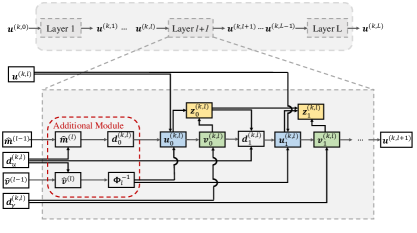
To derive a DNN with the above-mentioned properties, we unfold the MM-ADMM-based SN selection method and introduce an additional module. The new DNN is called DAN. As shown in Fig. 2, DAN consists of L𝐿L cascaded layers with some learnable parameters, where the (l+1)𝑙1(l+1)th layer takes the first- and second-order momentum 𝐦^(l1)superscript^𝐦𝑙1\hat{\mathbf{m}}^{(l-1)} and 𝐯^(l1)superscript^𝐯𝑙1\hat{\mathbf{v}}^{(l-1)}, the gradients 𝐝u(k,l)superscriptsubscript𝐝𝑢𝑘𝑙\mathbf{d}_{u}^{(k,l)} and 𝐝v(k,l)superscriptsubscript𝐝𝑣𝑘𝑙\mathbf{d}_{v}^{(k,l)}, and the output from the previous layer 𝐮(k,l)superscript𝐮𝑘𝑙\mathbf{u}^{(k,l)} as inputs, and outputs an update 𝐮(k,l+1)superscript𝐮𝑘𝑙1\mathbf{u}^{(k,l+1)}. In particular, the (l+1)𝑙1(l+1)th layer updates 𝐮m(k,l)superscriptsubscript𝐮𝑚𝑘𝑙\mathbf{u}_{m}^{(k,l)}, 𝐯m(k,l)superscriptsubscript𝐯𝑚𝑘𝑙\mathbf{v}_{m}^{(k,l)}, and 𝐳m(k,l)superscriptsubscript𝐳𝑚𝑘𝑙\mathbf{z}_{m}^{(k,l)}, alternatively, as shown by the blue, green, and orange blocks in Fig. 2, respectively. The update of 𝐮m+1(k,l)superscriptsubscript𝐮𝑚1𝑘𝑙\mathbf{u}_{m+1}^{(k,l)} is of the same form as (31). But we make the following two modifications, as shown by the red block in Fig. 2:
Refer to caption
Figure 2: Illustration of DAN.

1) 𝐝m(k,l)superscriptsubscript𝐝𝑚𝑘𝑙\mathbf{d}_{m}^{(k,l)} is constructed as

𝐝m(k,l)=𝐦^lρa,l(𝐯m(k,l)𝐳m(k,l)),superscriptsubscript𝐝𝑚𝑘𝑙subscript^𝐦𝑙subscript𝜌𝑎𝑙superscriptsubscript𝐯𝑚𝑘𝑙superscriptsubscript𝐳𝑚𝑘𝑙\begin{split}\mathbf{d}_{m}^{(k,l)}=\hat{\mathbf{m}}_{l}-\rho_{a,l}(\mathbf{v}_{m}^{(k,l)}-\mathbf{z}_{m}^{(k,l)}),\end{split} (35)

where

𝐦^l=β1,l𝐦^l1+(1β1,l)𝐝u(k,l).subscript^𝐦𝑙subscript𝛽1𝑙subscript^𝐦𝑙11subscript𝛽1𝑙superscriptsubscript𝐝𝑢𝑘𝑙\begin{split}\hat{\mathbf{m}}_{l}=\beta_{1,l}\hat{\mathbf{m}}_{l-1}+(1-\beta_{1,l})\mathbf{d}_{u}^{(k,l)}.\end{split} (36)

Here, β1,l=β1η1lsubscript𝛽1𝑙subscript𝛽1superscriptsubscript𝜂1𝑙\beta_{1,l}=\beta_{1}\eta_{1}^{l} where η1(0,1)subscript𝜂101\eta_{1}\in(0,1) and β1(0,1)subscript𝛽101\beta_{1}\in(0,1) denotes a learnable hyper-parameters to avoid the case that the momentum diverges severely.

When β1,l=0subscript𝛽1𝑙0\beta_{1,l}=0, the first-order momentum 𝐦^lsubscript^𝐦𝑙\hat{\mathbf{m}}_{l} reduces to the gradient 𝐝u(k,l)superscriptsubscript𝐝𝑢𝑘𝑙\mathbf{d}_{u}^{(k,l)}. In this paper, we define β1,l=β1η1lsubscript𝛽1𝑙subscript𝛽1superscriptsubscript𝜂1𝑙\beta_{1,l}=\beta_{1}\eta_{1}^{l} with β1(0,1)subscript𝛽101\beta_{1}\in(0,1) and η1(0,1)subscript𝜂101\eta_{1}\in(0,1). The momentum terms caused by non-zero β1,lsubscript𝛽1𝑙\beta_{1,l} may improve the performance significantly, especially in deep learning applications.

2) 𝚽lsubscript𝚽𝑙\mathbf{\Phi}_{l} is constructed as

𝚽l=𝐓^(k,l)+ρa,l𝐈,subscript𝚽𝑙superscript^𝐓𝑘𝑙subscript𝜌𝑎𝑙𝐈\mathbf{\Phi}_{l}=\hat{\mathbf{T}}^{(k,l)}+\rho_{a,l}\mathbf{I}, (37)

where 𝐓^(k,l)diag([|v^l,1|α1,l,,|v^l,N|α1,l]),superscript^𝐓𝑘𝑙diagsubscript^𝑣𝑙1subscript𝛼1𝑙subscript^𝑣𝑙𝑁subscript𝛼1𝑙\hat{\mathbf{T}}^{(k,l)}\triangleq\mathrm{diag}\left(\left[\frac{\sqrt{|\hat{v}_{l,1}|}}{\alpha_{1,l}},\cdots,\frac{\sqrt{|\hat{v}_{l,N}|}}{\alpha_{1,l}}\right]\right), and ρa,l=ρaηalsubscript𝜌𝑎𝑙subscript𝜌𝑎superscriptsubscript𝜂𝑎𝑙\rho_{a,l}=\rho_{a}\eta_{a}^{l} with ηal(0,1)superscriptsubscript𝜂𝑎𝑙01\eta_{a}^{l}\in(0,1). Here, v^l,isubscript^𝑣𝑙𝑖\hat{v}_{l,i} denotes the i𝑖ith entry of the second-order momentum 𝐯^lsubscript^𝐯𝑙\hat{\mathbf{v}}_{l}, which is defined by

𝐯^l=β2𝐯^l1+(1β2)(𝐝u(k,l))2,subscript^𝐯𝑙subscript𝛽2subscript^𝐯𝑙11subscript𝛽2superscriptsuperscriptsubscript𝐝𝑢𝑘𝑙2\hat{\mathbf{v}}_{l}=\beta_{2}\hat{\mathbf{v}}_{l-1}+(1-\beta_{2})(\mathbf{d}_{u}^{(k,l)})^{2}, (38)

where β2subscript𝛽2\beta_{2} denotes a constant to control the second-order momentum and α1,l=α¯1,llsubscript𝛼1𝑙subscript¯𝛼1𝑙𝑙\alpha_{1,l}=\frac{\bar{\alpha}_{1,l}}{\sqrt{l}} with α¯1,l[α1,α1+]subscript¯𝛼1𝑙superscriptsubscript𝛼1superscriptsubscript𝛼1\bar{\alpha}_{1,l}\in[\alpha_{1}^{-},\alpha_{1}^{+}] representing a set of learnable parameters to control the update step size. Here, the positive constants α1superscriptsubscript𝛼1\alpha_{1}^{-} and α1+superscriptsubscript𝛼1\alpha_{1}^{+} are the lower and upper bounds of α¯1,lsubscript¯𝛼1𝑙\bar{\alpha}_{1,l}. We refer to the diagonal element of 𝚽l1superscriptsubscript𝚽𝑙1\mathbf{\Phi}_{l}^{-1} as the learning rate of this algorithm, whose i𝑖ith entry is given by ϕl,i1=(|v^l,i|/α1,l+ρa,l)1superscriptsubscriptitalic-ϕ𝑙𝑖1superscriptsubscript^𝑣𝑙𝑖subscript𝛼1𝑙subscript𝜌𝑎𝑙1\phi_{l,i}^{-1}=\left({\sqrt{|\hat{v}_{l,i}|}}/{\alpha_{1,l}}+\rho_{a,l}\right)^{-1}. Learning rate decay is critical for training neural networks. In the early training stage, a large learning rate can accelerate training and help the network escape spurious local minima. By the end of the iteration, a small learning rate helps the network converge to a local minimum and avoid oscillation. Therefore, we desire a set of ρa,lsubscript𝜌𝑎𝑙\rho_{a,l} and α1,lsubscript𝛼1𝑙\alpha_{1,l} such that, for any l{2,,L}𝑙2𝐿l\in\{2,\cdots,L\} and i{1,,N}𝑖1𝑁i\in\{1,\cdots,N\}, we have ϕl,i1ϕl1,i1superscriptsubscriptitalic-ϕ𝑙𝑖1superscriptsubscriptitalic-ϕ𝑙1𝑖1\phi_{l,i}^{-1}\leq\phi_{l-1,i}^{-1}.

The updates are inspired by the adaptive momentum (Adam) method [37], i.e., an algorithm for first-order gradient-based optimization. Adam is chosen due to its favorable properties: 1) simple implementation, computationally efficient, and low memory requirements; 2) adaptability to large-scale problems; and 3) adaptation to sparse gradients [37]. Based on the adaptive estimates of first- and second-order momentum, we propose a novel construction of 𝐝m(k,l)superscriptsubscript𝐝𝑚𝑘𝑙\mathbf{d}_{m}^{(k,l)} and 𝐓^(k,l)superscript^𝐓𝑘𝑙\hat{\mathbf{T}}^{(k,l)} as well as its resultant 𝚽lsubscript𝚽𝑙\mathbf{\Phi}_{l}, which can meet the constraint in (15c) and the diagonal requirement, simultaneously. But different from ADAM, the update has additional terms resulting from the original MM-ADMM and one learnable step size α1,lsubscript𝛼1𝑙\alpha_{1,l} to control the iteration process. Compared with training all diagonal elements of 𝐓^(k,l)superscript^𝐓𝑘𝑙\hat{\mathbf{T}}^{(k,l)}, the learnable parameters in the DAN are changed to α¯1,lsubscript¯𝛼1𝑙\bar{\alpha}_{1,l} and β1subscript𝛽1\beta_{1}. The total number of learnable parameters over all layers is reduced from LN𝐿𝑁LN to L+1𝐿1L+1.

The update of 𝐯m+1(k,l)superscriptsubscript𝐯𝑚1𝑘𝑙\mathbf{v}_{m+1}^{(k,l)} and 𝐳m+1(k,l)superscriptsubscript𝐳𝑚1𝑘𝑙\mathbf{z}_{m+1}^{(k,l)} are the same as (33) and (28c), respectively. With given 𝐦^lsubscript^𝐦𝑙\hat{\mathbf{m}}_{l} and 𝚽lsubscript𝚽𝑙\mathbf{\Phi}_{l}, the Lagrange function (𝐮(k),𝐯(k),𝐳(k)|𝐦^l,𝚽l)superscript𝐮𝑘superscript𝐯𝑘conditionalsuperscript𝐳𝑘subscript^𝐦𝑙subscript𝚽𝑙\mathcal{L}(\mathbf{u}^{(k)},\mathbf{v}^{(k)},\mathbf{z}^{(k)}|\hat{\mathbf{m}}_{l},\mathbf{\Phi}_{l}) defined in (27) will not increase after updating 𝐮m(k,l)superscriptsubscript𝐮𝑚𝑘𝑙\mathbf{u}_{m}^{(k,l)}, 𝐯m(k,l)superscriptsubscript𝐯𝑚𝑘𝑙\mathbf{v}_{m}^{(k,l)} and 𝐳m(k,l)superscriptsubscript𝐳𝑚𝑘𝑙\mathbf{z}_{m}^{(k,l)} by (31), (33), and (28c), respectively. The modified ADMM iteration will also converge at a set of station points denoted by 𝐮()(k)superscriptsubscript𝐮𝑘\mathbf{u}_{(\star)}^{(k)}, 𝐯()(k)superscriptsubscript𝐯𝑘\mathbf{v}_{(\star)}^{(k)}, and 𝐳()(k)superscriptsubscript𝐳𝑘\mathbf{z}_{(\star)}^{(k)}. Therefore, we have

𝐮(k,l+1)=𝐮(k,l)=𝐮(k,l)𝚽l1(𝐝(k,l)νl𝟏),superscript𝐮𝑘𝑙1superscriptsubscript𝐮𝑘𝑙superscript𝐮𝑘𝑙superscriptsubscript𝚽𝑙1superscriptsubscript𝐝𝑘𝑙subscript𝜈𝑙1\begin{split}&\mathbf{u}^{(k,l+1)}=\mathbf{u}_{\star}^{(k,l)}=\mathbf{u}^{(k,l)}-\mathbf{\Phi}_{l}^{-1}\left(\mathbf{d}_{\star}^{(k,l)}-\nu_{l}\mathbf{1}\right),\end{split} (39)

where

𝐝(k,l)=𝐦^lρa,l(𝐯(k,l)𝐳(k,l)),νl=𝟏T𝚽l1𝐝(k,l)𝟏T𝚽l1𝟏.formulae-sequencesuperscriptsubscript𝐝𝑘𝑙subscript^𝐦𝑙subscript𝜌𝑎𝑙superscriptsubscript𝐯𝑘𝑙superscriptsubscript𝐳𝑘𝑙subscript𝜈𝑙superscript1Tsuperscriptsubscript𝚽𝑙1superscriptsubscript𝐝𝑘𝑙superscript1Tsuperscriptsubscript𝚽𝑙11\mathbf{d}_{\star}^{(k,l)}=\hat{\mathbf{m}}_{l}-\rho_{a,l}(\mathbf{v}_{\star}^{(k,l)}-\mathbf{z}_{\star}^{(k,l)}),\;\nu_{l}=\frac{\mathbf{1}^{\mathrm{T}}\mathbf{\Phi}_{l}^{-1}\mathbf{d}_{\star}^{(k,l)}}{\mathbf{1}^{\mathrm{T}}\mathbf{\Phi}_{l}^{-1}\mathbf{1}}. (40)

III-C Convergence of DAN

Until now, we have developed a new model-driven method for SN selection. However, the obtained 𝐓^(k,l)superscript^𝐓𝑘𝑙\hat{\mathbf{T}}^{(k,l)} may not satisfy (23), which indicates that the convergence property of the MM framework is questionable. To address this issue, we next analyze the convergence of the proposed DAN.

For any sequence {𝐮(k,l)}l=1Lsuperscriptsubscriptsuperscript𝐮𝑘𝑙𝑙1𝐿\{\mathbf{u}^{(k,l)}\}_{l=1}^{L} generated by the proposed DAN, the regret function is defined as

RLl=1L(𝒢(𝐮(k,l))𝒢(𝐮(k,))),subscript𝑅𝐿superscriptsubscript𝑙1𝐿𝒢superscript𝐮𝑘𝑙𝒢superscript𝐮𝑘\begin{split}R_{L}\triangleq\sum\limits_{l=1}^{L}\left(\mathcal{G}(\mathbf{u}^{(k,l)})-\mathcal{G}(\mathbf{u}^{(k,\star)})\right),\end{split} (41)

where 𝐮(k,)=argmin𝐮(k)𝒮u𝒢(𝐮(k))superscript𝐮𝑘subscriptsuperscript𝐮𝑘subscript𝒮𝑢𝒢superscript𝐮𝑘\mathbf{u}^{(k,\star)}=\arg\min_{\mathbf{u}^{(k)}\in\mathcal{S}_{u}}\mathcal{G}(\mathbf{u}^{(k)}) denotes the best stationary point in the feasible set 𝒮usubscript𝒮𝑢\mathcal{S}_{u}. Generally speaking, the regret function indicates the sum of the difference between 𝒢(𝐮(k,l))𝒢superscript𝐮𝑘𝑙\mathcal{G}(\mathbf{u}^{(k,l)}) and 𝒢(𝐮(k,))𝒢superscript𝐮𝑘\mathcal{G}(\mathbf{u}^{(k,\star)}), which is widely used for the convergence proof [37]. Note that the feasible set has bounded diameter, i.e., for all 𝐮,𝐯𝒮u𝐮𝐯subscript𝒮𝑢\mathbf{u},\mathbf{v}\in\mathcal{S}_{u}, 𝐮𝐯2DΔsuperscriptnorm𝐮𝐯2subscript𝐷Δ||\mathbf{u}-\mathbf{v}||^{2}\leq D_{\Delta}. Define Du,1maxl𝐝u(k,l)1subscript𝐷𝑢1subscript𝑙subscriptnormsuperscriptsubscript𝐝𝑢𝑘𝑙1D_{u,1}\triangleq\max\limits_{l}||\mathbf{d}_{u}^{(k,l)}||_{1}, Dϕmaxlmaxiϕl,i1subscript𝐷italic-ϕsubscript𝑙subscript𝑖superscriptsubscriptitalic-ϕ𝑙𝑖1D_{\phi}\triangleq\max\limits_{l}\max\limits_{i}\phi_{l,i}^{-1}, Db,1maxl𝐛^l1subscript𝐷𝑏1subscript𝑙subscriptnormsubscript^𝐛𝑙1D_{b,1}\triangleq\max_{l}||\hat{\mathbf{b}}_{l}||_{1}, and Db,2maxl𝐛^l2subscript𝐷𝑏2subscript𝑙superscriptnormsubscript^𝐛𝑙2D_{b,2}\triangleq\max_{l}||\hat{\mathbf{b}}_{l}||^{2}, where 𝐛^l=𝐯(k,l)𝐳(k,l)subscript^𝐛𝑙superscriptsubscript𝐯𝑘𝑙superscriptsubscript𝐳𝑘𝑙\hat{\mathbf{b}}_{l}=\mathbf{v}_{\star}^{(k,l)}-\mathbf{z}_{\star}^{(k,l)}. Then, we have the following theorem for the convergence analysis.

Theorem 1

Assume that, for all l[2,L]𝑙2𝐿l\in[2,L], ϕl,i1ϕl1,i1superscriptsubscriptitalic-ϕ𝑙𝑖1superscriptsubscriptitalic-ϕ𝑙1𝑖1\phi_{l,i}^{-1}\leq\phi_{l-1,i}^{-1}. The regret is bounded by

RLC1L+C2,subscript𝑅𝐿subscript𝐶1𝐿subscript𝐶2\begin{split}&R_{L}\leq C_{1}\sqrt{L}+C_{2},\end{split} (42)

where C1=1β2Du,1DΔα1(1β2)(1β1)subscript𝐶11subscript𝛽2subscript𝐷𝑢1subscript𝐷Δsuperscriptsubscript𝛼11subscript𝛽21subscript𝛽1C_{1}=\frac{\sqrt{1-\beta_{2}}D_{u,1}D_{\Delta}}{\alpha_{1}^{-}(1-\sqrt{\beta_{2}})(1-\beta_{1})} and C2subscript𝐶2C_{2} is defined by (43), given at the top of this page.

Proof: See Appendix A. \blacksquare

Since C1subscript𝐶1C_{1} and C2subscript𝐶2C_{2} are constants independent of L𝐿L, Theorem 1 indicates that the DAN has a regret of 𝒪(L12)𝒪superscript𝐿12\mathcal{O}(L^{\frac{1}{2}}), which guarantees that the sequence {𝒢(𝐮(k,l))}l=1Lsuperscriptsubscript𝒢superscript𝐮𝑘𝑙𝑙1𝐿\{\mathcal{G}(\mathbf{u}^{(k,l)})\}_{l=1}^{L} will converge to 𝒢(𝐮(k,))𝒢superscript𝐮𝑘\mathcal{G}(\mathbf{u}^{(k,\star)}) with convergence rate on the order of 𝒪(L12)𝒪superscript𝐿12\mathcal{O}(L^{-\frac{1}{2}}).

C2=2ρaDΔηa1β1+1β2Du,1DΔα1(1β2)(1β1)+α1+(3+β1)Du,12(1β1)2(1β1β2)1β2(1η12)+ρaDϕ(Db,1+Db,2)2(1ηa)(1β1)subscript𝐶22subscript𝜌𝑎subscript𝐷Δsubscript𝜂𝑎1subscript𝛽11subscript𝛽2subscript𝐷𝑢1subscript𝐷Δsuperscriptsubscript𝛼11subscript𝛽21subscript𝛽1superscriptsubscript𝛼13subscript𝛽1subscript𝐷𝑢12superscript1subscript𝛽121subscript𝛽1subscript𝛽21subscript𝛽21superscriptsubscript𝜂12subscript𝜌𝑎subscript𝐷italic-ϕsubscript𝐷𝑏1subscript𝐷𝑏221subscript𝜂𝑎1subscript𝛽1\displaystyle C_{2}=\frac{2\rho_{a}D_{\Delta}\eta_{a}}{1-\beta_{1}}+\frac{\sqrt{1-\beta_{2}}D_{u,1}D_{\Delta}}{\alpha_{1}^{-}(1-\sqrt{\beta_{2}})(1-\beta_{1})}+\frac{\alpha_{1}^{+}(3+\beta_{1})D_{u,1}}{2(1-\beta_{1})^{2}(1-\frac{\beta_{1}}{\sqrt{\beta_{2}}})\sqrt{1-\beta_{2}}(1-\eta_{1}^{2})}+\frac{\rho_{a}D_{\phi}(D_{b,1}+D_{b,2})}{2(1-\eta_{a})(1-\beta_{1})}
+Du,1Dϕ2(1η1)(1β1)2+β11β2Du,1DΔ2α1(1β2)(1η1)2(1β1)+β1ρaDΔ2(1η1ηa)(1β1)+ρa1β2Du,1DΔ2α1(1β2)(1ηa)2(1β1)subscript𝐷𝑢1subscript𝐷italic-ϕ21subscript𝜂1superscript1subscript𝛽12subscript𝛽11subscript𝛽2subscript𝐷𝑢1subscript𝐷Δ2superscriptsubscript𝛼11subscript𝛽2superscript1subscript𝜂121subscript𝛽1subscript𝛽1subscript𝜌𝑎subscript𝐷Δ21subscript𝜂1subscript𝜂𝑎1subscript𝛽1subscript𝜌𝑎1subscript𝛽2subscript𝐷𝑢1subscript𝐷Δ2superscriptsubscript𝛼11subscript𝛽2superscript1subscript𝜂𝑎21subscript𝛽1\displaystyle+\frac{D_{u,1}D_{\phi}}{2(1-\eta_{1})(1-\beta_{1})^{2}}+\frac{\beta_{1}\sqrt{1-\beta_{2}}D_{u,1}D_{\Delta}}{2\alpha_{1}^{-}(1-\sqrt{\beta_{2}})(1-\eta_{1})^{2}(1-\beta_{1})}+\frac{\beta_{1}\rho_{a}D_{\Delta}}{2(1-\eta_{1}\eta_{a})(1-\beta_{1})}+\frac{\rho_{a}\sqrt{1-\beta_{2}}D_{u,1}D_{\Delta}}{2\alpha_{1}^{-}(1-\sqrt{\beta_{2}})(1-\eta_{a})^{2}(1-\beta_{1})}
+ρa2DΔ2(1ηa2)(1β1)+3ρa2DϕDb,22(1ηa2)(1β1)+3Du,12Dϕ(1η12)(1β1)3+3ρa2Db,12Dϕ(1ηa2)(1β1)+DΔu,2Dϕ1β1superscriptsubscript𝜌𝑎2subscript𝐷Δ21superscriptsubscript𝜂𝑎21subscript𝛽13superscriptsubscript𝜌𝑎2subscript𝐷italic-ϕsubscript𝐷𝑏221superscriptsubscript𝜂𝑎21subscript𝛽13superscriptsubscript𝐷𝑢12subscript𝐷italic-ϕ1superscriptsubscript𝜂12superscript1subscript𝛽133superscriptsubscript𝜌𝑎2superscriptsubscript𝐷𝑏12subscript𝐷italic-ϕ1superscriptsubscript𝜂𝑎21subscript𝛽1subscript𝐷subscriptΔ𝑢2subscript𝐷italic-ϕ1subscript𝛽1\displaystyle+\frac{\rho_{a}^{2}D_{\Delta}}{2(1-\eta_{a}^{2})(1-\beta_{1})}+\frac{3\rho_{a}^{2}D_{\phi}D_{b,2}}{2(1-\eta_{a}^{2})(1-\beta_{1})}+\frac{3D_{u,1}^{2}D_{\phi}}{(1-\eta_{1}^{2})(1-\beta_{1})^{3}}+\frac{3\rho_{a}^{2}D_{b,1}^{2}D_{\phi}}{(1-\eta_{a}^{2})(1-\beta_{1})}+\frac{D_{\Delta_{u,2}}D_{\phi}}{1-\beta_{1}} (43)
+[Du,1(1β1)(1η1)2+ρaDb,1(1ηa)2]1β2Du,1DΔ2α1(1β2)(1β1)+[Du,1(1β1)(1η1)(1ηa)+ρaDb,1(1ηa)2]DΔρa2(1β1).delimited-[]subscript𝐷𝑢11subscript𝛽1superscript1subscript𝜂12subscript𝜌𝑎subscript𝐷𝑏1superscript1subscript𝜂𝑎21subscript𝛽2subscript𝐷𝑢1subscript𝐷Δ2superscriptsubscript𝛼11subscript𝛽21subscript𝛽1delimited-[]subscript𝐷𝑢11subscript𝛽11subscript𝜂11subscript𝜂𝑎subscript𝜌𝑎subscript𝐷𝑏1superscript1subscript𝜂𝑎2subscript𝐷Δsubscript𝜌𝑎21subscript𝛽1\displaystyle+\left[\frac{D_{u,1}}{(1-\beta_{1})(1-\eta_{1})^{2}}+\frac{\rho_{a}D_{b,1}}{(1-\eta_{a})^{2}}\right]\frac{\sqrt{1-\beta_{2}}D_{u,1}D_{\Delta}}{2\alpha_{1}^{-}(1-\sqrt{\beta_{2}})(1-\beta_{1})}+\left[\frac{D_{u,1}}{(1-\beta_{1})(1-\eta_{1})(1-\eta_{a})}+\frac{\rho_{a}D_{b,1}}{(1-\eta_{a})^{2}}\right]\frac{D_{\Delta}\rho_{a}}{2(1-\beta_{1})}.

III-D Transmit Power Allocation For Multiple Targets

Given {𝐮q(k,j+1)}q=1Qsuperscriptsubscriptsuperscriptsubscript𝐮𝑞𝑘𝑗1𝑞1𝑄\{{\mathbf{u}}_{q}^{(k,j+1)}\}_{q=1}^{Q}, the problem in (17) can be expressed as

min𝐩(k)𝒮pq=1Qpa(pq(k)),subscriptsuperscript𝐩𝑘subscript𝒮𝑝superscriptsubscript𝑞1𝑄subscriptpasuperscriptsubscript𝑝𝑞𝑘\begin{split}\min_{\mathbf{p}^{(k)}\in\mathcal{S}_{p}}\;&\sum_{q=1}^{Q}\mathcal{F}_{\mathrm{pa}}(p_{q}^{(k)}),\\ \end{split} (44)

where pa(pq(k))=logdet𝐂q(pq(k)|𝐮q(k,j))subscriptpasuperscriptsubscript𝑝𝑞𝑘subscript𝐂𝑞conditionalsuperscriptsubscript𝑝𝑞𝑘superscriptsubscript𝐮𝑞𝑘𝑗\mathcal{F}_{\mathrm{pa}}(p_{q}^{(k)})=\log\det\mathbf{C}_{q}(p_{q}^{(k)}|\mathbf{u}_{q}^{(k,j)}) is the cost function and 𝒮p={𝐩(k)|q=1Qpq(k)PT,pq(k)Pmin,q=1,2,Q}subscript𝒮𝑝conditional-setsuperscript𝐩𝑘formulae-sequencesuperscriptsubscript𝑞1𝑄superscriptsubscript𝑝𝑞𝑘subscript𝑃𝑇formulae-sequencesuperscriptsubscript𝑝𝑞𝑘subscript𝑃𝑞12𝑄\mathcal{S}_{p}=\{\mathbf{p}^{(k)}|\sum_{q=1}^{Q}p_{q}^{(k)}\leq P_{T},p_{q}^{(k)}\geq P_{\min},q=1,2\cdots,Q\} denotes the feasible set of 𝐩(k)superscript𝐩𝑘\mathbf{p}^{(k)}. This problem is convex and can be reformulated as a SDP problem, i.e.,

max𝐩(k)q=1Qlogdet(𝐐q),s.t.q=1Qpq(k)PT,pq(k)Pmin,𝐉q(k)(pq(k)|𝐮q(k,j))𝐐q,q=1,2,Q,\begin{split}\max_{\mathbf{p}^{(k)}}\;&\sum_{q=1}^{Q}\log\det(\mathbf{Q}_{q}),\\ \text{s.t.}\;&\sum_{q=1}^{Q}p_{q}^{(k)}\leq P_{T},\quad p_{q}^{(k)}\geq P_{\min},\\ &\mathbf{J}_{q}^{(k)}(p_{q}^{(k)}|\mathbf{u}_{q}^{(k,j)})\succeq\mathbf{Q}_{q},q=1,2\cdots,Q,\end{split} (45)

where {𝐐q}q=1Qsuperscriptsubscriptsubscript𝐐𝑞𝑞1𝑄\{\mathbf{Q}_{q}\}_{q=1}^{Q} denotes a set of auxiliary symmetric matrices. Then, this problem can be solved by the CVX toolbox.

However, the CVX toolbox is generally time-consuming, especially when the number of targets is large. To reduce the computational complexity and reveal more physical insights, we propose an iterative water-filling-based power allocation method. First, we merge the total power constraint into the cost function by the Lagrange multiplier method, i.e.,

pa(𝐩(k))=q=1Qpa(pq(k))+λpa(PTq=1Qpq(k)),subscriptpasuperscript𝐩𝑘superscriptsubscript𝑞1𝑄subscriptpasuperscriptsubscript𝑝𝑞𝑘subscript𝜆pasubscript𝑃𝑇superscriptsubscript𝑞1𝑄superscriptsubscript𝑝𝑞𝑘\begin{split}\mathcal{L}_{\mathrm{pa}}(\mathbf{p}^{(k)})&=\sum_{q=1}^{Q}\mathcal{F}_{\mathrm{pa}}(p_{q}^{(k)})+\lambda_{\mathrm{pa}}(P_{T}-\sum_{q=1}^{Q}p_{q}^{(k)}),\end{split} (46)

where λpasubscript𝜆pa\lambda_{\mathrm{pa}} is the Lagrange multiplier. The derivative of (46) w.r.t. pq(k)superscriptsubscript𝑝𝑞𝑘p_{q}^{(k)} is given by

pa(𝐩(k))pq(k)=tr((𝐉P,q(k)+pq(k)𝚺~q(k))1𝚺~q(k))λpa,subscriptpasuperscript𝐩𝑘superscriptsubscript𝑝𝑞𝑘trsuperscriptsuperscriptsubscript𝐉𝑃𝑞𝑘superscriptsubscript𝑝𝑞𝑘superscriptsubscript~𝚺𝑞𝑘1superscriptsubscript~𝚺𝑞𝑘subscript𝜆pa\begin{split}\frac{\partial\mathcal{L}_{\mathrm{pa}}(\mathbf{p}^{(k)})}{\partial p_{q}^{(k)}}=\mathrm{tr}((\mathbf{J}_{P,q}^{(k)}+p_{q}^{(k)}\widetilde{\mathbf{\Sigma}}_{q}^{(k)})^{-1}\widetilde{\mathbf{\Sigma}}_{q}^{(k)})-\lambda_{\mathrm{pa}},\end{split} (47)

where 𝚺~q(k)=n=1Nuq,n(k)𝐌¯q,n(k).superscriptsubscript~𝚺𝑞𝑘superscriptsubscript𝑛1𝑁superscriptsubscript𝑢𝑞𝑛𝑘superscriptsubscript¯𝐌𝑞𝑛𝑘\widetilde{\mathbf{\Sigma}}_{q}^{(k)}=\sum_{n=1}^{N}u_{q,n}^{(k)}\overline{\mathbf{M}}_{q,n}^{(k)}. By setting pa(𝐩(k))pq(k)=0subscriptpasuperscript𝐩𝑘superscriptsubscript𝑝𝑞𝑘0\frac{\partial\mathcal{L}_{\mathrm{pa}}(\mathbf{p}^{(k)})}{\partial p_{q}^{(k)}}=0, we have the following fixed-point equation, i.e.,

pq(k)=1λpatr(𝐉P,q(k)+pq(k)𝚺~q(k))1𝐉P,q(k)tr(𝐉P,q(k)+pq(k)𝚺~q(k))1𝚺~q(k).superscriptsubscript𝑝𝑞𝑘1subscript𝜆patrsuperscriptsuperscriptsubscript𝐉𝑃𝑞𝑘superscriptsubscript𝑝𝑞𝑘superscriptsubscript~𝚺𝑞𝑘1superscriptsubscript𝐉𝑃𝑞𝑘trsuperscriptsuperscriptsubscript𝐉𝑃𝑞𝑘superscriptsubscript𝑝𝑞𝑘superscriptsubscript~𝚺𝑞𝑘1superscriptsubscript~𝚺𝑞𝑘\begin{split}p_{q}^{(k)}=\frac{1}{\lambda_{\mathrm{pa}}}-\frac{\mathrm{tr}\;(\mathbf{J}_{P,q}^{(k)}+p_{q}^{(k)}\widetilde{\mathbf{\Sigma}}_{q}^{(k)})^{-1}\mathbf{J}_{P,q}^{(k)}}{\mathrm{tr}\;(\mathbf{J}_{P,q}^{(k)}+p_{q}^{(k)}\widetilde{\mathbf{\Sigma}}_{q}^{(k)})^{-1}\widetilde{\mathbf{\Sigma}}_{q}^{(k)}}.\end{split} (48)

If 𝐉P,q(k)superscriptsubscript𝐉𝑃𝑞𝑘\mathbf{J}_{P,q}^{(k)} and 𝚺~q(k)superscriptsubscript~𝚺𝑞𝑘\widetilde{\mathbf{\Sigma}}_{q}^{(k)} reduce to one-dimensional constants denoted by JP,q(k)superscriptsubscript𝐽𝑃𝑞𝑘{J}_{P,q}^{(k)} and Σ~q(k)superscriptsubscript~Σ𝑞𝑘\widetilde{{\Sigma}}_{q}^{(k)}, respectively, the closed-form solution of pq(k)superscriptsubscript𝑝𝑞𝑘p_{q}^{(k)} can be directly obtained from (48), i.e., pq(k)=μwfJP,q(k)/Σ~q(k)superscriptsubscript𝑝𝑞𝑘subscript𝜇wfsuperscriptsubscript𝐽𝑃𝑞𝑘superscriptsubscript~Σ𝑞𝑘p_{q}^{(k)}=\mu_{\mathrm{wf}}-{{J}_{P,q}^{(k)}}/{\widetilde{{\Sigma}}_{q}^{(k)}}, where μwf=1λpasubscript𝜇wf1subscript𝜆pa\mu_{\mathrm{wf}}=\frac{1}{\lambda_{\mathrm{pa}}} denotes the water level. For the matrix-version 𝐉P,q(k)superscriptsubscript𝐉𝑃𝑞𝑘\mathbf{J}_{P,q}^{(k)} and 𝚺~q(k)superscriptsubscript~𝚺𝑞𝑘\widetilde{\mathbf{\Sigma}}_{q}^{(k)}, we propose to obtain pq(k)superscriptsubscript𝑝𝑞𝑘p_{q}^{(k)} and the water level μwfsubscript𝜇wf\mu_{\mathrm{wf}} by an iteration process. In particular, at the i𝑖ith iteration, pq,i+1(k)superscriptsubscript𝑝𝑞𝑖1𝑘p_{q,i+1}^{(k)} is obtained by

pq,i+1(k)=μwftr(𝐉P,q(k)+pq,i(k)𝚺~q(k))1𝐉P,q(k)tr(𝐉P,q(k)+pq,i(k)𝚺~q(k))1𝚺~q(k)Pmin,superscriptsubscript𝑝𝑞𝑖1𝑘subscriptsubscript𝜇wftrsuperscriptsuperscriptsubscript𝐉𝑃𝑞𝑘superscriptsubscript𝑝𝑞𝑖𝑘superscriptsubscript~𝚺𝑞𝑘1superscriptsubscript𝐉𝑃𝑞𝑘trsuperscriptsuperscriptsubscript𝐉𝑃𝑞𝑘superscriptsubscript𝑝𝑞𝑖𝑘superscriptsubscript~𝚺𝑞𝑘1superscriptsubscript~𝚺𝑞𝑘subscript𝑃p_{q,i+1}^{(k)}=\left\lfloor\mu_{\mathrm{wf}}-\frac{\mathrm{tr}\;(\mathbf{J}_{P,q}^{(k)}+p_{q,i}^{(k)}\widetilde{\mathbf{\Sigma}}_{q}^{(k)})^{-1}\mathbf{J}_{P,q}^{(k)}}{\mathrm{tr}\;(\mathbf{J}_{P,q}^{(k)}+p_{q,i}^{(k)}\widetilde{\mathbf{\Sigma}}_{q}^{(k)})^{-1}\widetilde{\mathbf{\Sigma}}_{q}^{(k)}}\right\rfloor_{P_{\min}}, (49)

where pq,i(k)superscriptsubscript𝑝𝑞𝑖𝑘p_{q,i}^{(k)} denotes the power for the q𝑞qth target at the i𝑖ith iteration and ab=max{a,b}subscript𝑎𝑏𝑎𝑏\left\lfloor a\right\rfloor_{b}=\max\{a,b\}. Then, the water level μwfsubscript𝜇wf\mu_{\mathrm{wf}} is updated by setting q=1Qpq,i+1(k)(μwf)=PT.superscriptsubscript𝑞1𝑄superscriptsubscript𝑝𝑞𝑖1𝑘subscript𝜇wfsubscript𝑃𝑇\sum_{q=1}^{Q}p_{q,i+1}^{(k)}(\mu_{\mathrm{wf}})=P_{T}.

Remark 3

According to the Rayleigh quotient, we have λ~mintr(𝐉P,q(k)+pq(k)𝚺~q(k))1𝐉P,q(k)tr(𝐉P,q(k)+pq(k)𝚺~q(k))1𝚺~q(k)λ~maxsubscript~𝜆trsuperscriptsuperscriptsubscript𝐉𝑃𝑞𝑘superscriptsubscript𝑝𝑞𝑘superscriptsubscript~𝚺𝑞𝑘1superscriptsubscript𝐉𝑃𝑞𝑘trsuperscriptsuperscriptsubscript𝐉𝑃𝑞𝑘superscriptsubscript𝑝𝑞𝑘superscriptsubscript~𝚺𝑞𝑘1superscriptsubscript~𝚺𝑞𝑘subscript~𝜆\tilde{\lambda}_{\min}\leq\frac{\mathrm{tr}\;(\mathbf{J}_{P,q}^{(k)}+p_{q}^{(k)}\widetilde{\mathbf{\Sigma}}_{q}^{(k)})^{-1}\mathbf{J}_{P,q}^{(k)}}{\mathrm{tr}\;(\mathbf{J}_{P,q}^{(k)}+p_{q}^{(k)}\widetilde{\mathbf{\Sigma}}_{q}^{(k)})^{-1}\widetilde{\mathbf{\Sigma}}_{q}^{(k)}}\leq\tilde{\lambda}_{\max}, where λ~minsubscript~𝜆\tilde{\lambda}_{\min} and λ~maxsubscript~𝜆\tilde{\lambda}_{\max} denote the minimum and maximum eigenvalue of (𝚺~q(k))1𝐉P,q(k)superscriptsuperscriptsubscript~𝚺𝑞𝑘1superscriptsubscript𝐉𝑃𝑞𝑘(\widetilde{\mathbf{\Sigma}}_{q}^{(k)})^{-1}\mathbf{J}_{P,q}^{(k)}, respectively. Note that 𝐉P,q(k)superscriptsubscript𝐉𝑃𝑞𝑘\mathbf{J}_{P,q}^{(k)} and 𝚺~q(k)superscriptsubscript~𝚺𝑞𝑘\widetilde{\mathbf{\Sigma}}_{q}^{(k)} denote the FIM of the prediction and the measurement, respectively. Thus, the eigenvalues of (𝚺~q(k))1𝐉P,q(k)superscriptsuperscriptsubscript~𝚺𝑞𝑘1superscriptsubscript𝐉𝑃𝑞𝑘(\widetilde{\mathbf{\Sigma}}_{q}^{(k)})^{-1}\mathbf{J}_{P,q}^{(k)} denote the ratio between the prediction and measurement. Recalling (48), if the eigenvalues of (𝚺~q(k))1𝐉P,q(k)superscriptsuperscriptsubscript~𝚺𝑞𝑘1superscriptsubscript𝐉𝑃𝑞𝑘(\widetilde{\mathbf{\Sigma}}_{q}^{(k)})^{-1}\mathbf{J}_{P,q}^{(k)} are larger, pq(k)superscriptsubscript𝑝𝑞𝑘p_{q}^{(k)} will be lower. This indicates that, more power will be allocated to a target, if 1) the measurement provides more information than the prediction, which enables the system to improve the accuracy of the prediction, or 2) the prediction of this target is so bad such that the system needs to allocate more power for better motion state estimation. In turn, if the eigenvalues of (𝚺~q(k))1𝐉P,q(k)superscriptsuperscriptsubscript~𝚺𝑞𝑘1superscriptsubscript𝐉𝑃𝑞𝑘(\widetilde{\mathbf{\Sigma}}_{q}^{(k)})^{-1}\mathbf{J}_{P,q}^{(k)} are smaller, pq(k)superscriptsubscript𝑝𝑞𝑘p_{q}^{(k)} will be lower. This indicates that, a target will be assigned with a lower power, if 1) the prediction is good enough; or 2) the measurement is too bad.

IV Simulation

In the simulation, we will show the efficiency and effectiveness of the proposed DAN and FP-WF algorithms. In the following, we first introduce the system parameters, the training details of DAN, and the benchmark algorithms.

System parameters: We consider a mmWave system operating at a carrier frequency of 28 GHz. There is one BS acting as the transmitter, which is located at [0,0]00[0,0] m. The number of SNs is N=32𝑁32N=32. These SNs are uniformly distributed in the area within 400×400400400400\times 400 m2superscriptm2\text{m}^{2}. On average, there is one SN within an area of 5000 m2superscriptm2\text{m}^{2}. The measurement covariance defined in (7) is generated by 𝚺q,n(k)=1SNRq(k)𝚺˙q,n(k)superscriptsubscript𝚺𝑞𝑛𝑘1superscriptsubscriptSNR𝑞𝑘superscriptsubscript˙𝚺𝑞𝑛𝑘\mathbf{\Sigma}_{q,n}^{(k)}=\frac{1}{\mathrm{SNR}_{q}^{(k)}}\dot{\mathbf{\Sigma}}_{q,n}^{(k)}, where 𝚺˙q,n(k)=diag[σ˙θq,n(k)2,σ˙τq,n(k)2,σ˙μq,n(k)2]superscriptsubscript˙𝚺𝑞𝑛𝑘diagsuperscriptsubscript˙𝜎superscriptsubscript𝜃𝑞𝑛𝑘2superscriptsubscript˙𝜎superscriptsubscript𝜏𝑞𝑛𝑘2superscriptsubscript˙𝜎superscriptsubscript𝜇𝑞𝑛𝑘2\dot{\mathbf{\Sigma}}_{q,n}^{(k)}=\mathrm{diag}[\dot{\sigma}_{\theta_{q,n}^{(k)}}^{2},\dot{\sigma}_{\tau_{q,n}^{(k)}}^{2},\dot{\sigma}_{\mu_{q,n}^{(k)}}^{2}] with σ˙θq,n(k)=2subscript˙𝜎superscriptsubscript𝜃𝑞𝑛𝑘2\dot{\sigma}_{\theta_{q,n}^{(k)}}=2, σ˙τq,n(k)=1subscript˙𝜎superscriptsubscript𝜏𝑞𝑛𝑘1\dot{\sigma}_{\tau_{q,n}^{(k)}}=1, σ˙μq,n(k)=1subscript˙𝜎superscriptsubscript𝜇𝑞𝑛𝑘1\dot{\sigma}_{\mu_{q,n}^{(k)}}=1. The SNR is defined by SNRq(k)=pq(k)γ0σ2(dq,n(k))2,superscriptsubscriptSNR𝑞𝑘superscriptsubscript𝑝𝑞𝑘subscript𝛾0superscript𝜎2superscriptsuperscriptsubscript𝑑𝑞𝑛𝑘2\mathrm{SNR}_{q}^{(k)}=\frac{p_{q}^{(k)}\gamma_{0}}{\sigma^{2}(d_{q,n}^{(k)})^{2}}, where γ0=61.4subscript𝛾061.4\gamma_{0}=-61.4 dB denotes the pathloss at reference distance. We set the total power at BS P=30𝑃30P=30 dBm, the minimum power for single target Pmin=20subscript𝑃𝑚𝑖𝑛20P_{min}=20 dBm, the noise power σ2=90superscript𝜎290\sigma^{2}=-90 dBm, the intensity of process noise qs=5subscript𝑞𝑠5q_{s}=5, and ΔT=0.5Δ𝑇0.5\Delta T=0.5 s.

Initialization of motion state: There are three targets to be tracked, i.e., Q=3𝑄3Q=3, if not otherwise specified. The initial velocities of the targets are given as 𝐯1=[10,0]Tsubscript𝐯1superscript100T\mathbf{v}_{1}=[-10,0]^{\mathrm{T}} m/s, 𝐯2=[0,10]Tsubscript𝐯2superscript010T\mathbf{v}_{2}=[0,-10]^{\mathrm{T}} m/s, 𝐯3=[10,0]Tsubscript𝐯3superscript100T\mathbf{v}_{3}=[10,0]^{\mathrm{T}} m/s, respectively. The initial locations of the targets are given as 𝐱1(0)=[124,124]Tsuperscriptsubscript𝐱10superscript124124T\mathbf{x}_{1}^{(0)}=[124,124]^{\mathrm{T}} m, 𝐱2(0)=[134,134]Tsuperscriptsubscript𝐱20superscript134134T\mathbf{x}_{2}^{(0)}=[-134,134]^{\mathrm{T}} m, and 𝐱3(0)=[144,144]Tsuperscriptsubscript𝐱30superscript144144T\mathbf{x}_{3}^{(0)}=[-144,-144]^{\mathrm{T}} m, respectively.

Training details: During training, the learnable parameters are optimized by the SGD optimizer in the PyTorch with a learning rate 5×1055superscript1055\times 10^{-5}. In our experiment, the loss function for training is selected as floss=1Ll=1L𝐮ES𝐮^l2,subscript𝑓𝑙𝑜𝑠𝑠1𝐿superscriptsubscript𝑙1𝐿superscriptnormsubscript𝐮𝐸𝑆superscript^𝐮𝑙2f_{loss}=\frac{1}{L}\sum_{l=1}^{L}||\mathbf{u}_{ES}-\hat{\mathbf{u}}^{l}||^{2}, where 𝐮ESsubscript𝐮𝐸𝑆\mathbf{u}_{ES} denotes the selection vector obtained by the exhaustive search (ES). The number of data for training is set as Ntrain=500subscript𝑁train500N_{\text{train}}=500. The network parameters are set as ρ=1𝜌1\rho=1, ρa=102subscript𝜌𝑎superscript102\rho_{a}=10^{2}, γ=104𝛾superscript104\gamma=10^{4}, β2=0.999subscript𝛽20.999\beta_{2}=0.999, η1=0.99subscript𝜂10.99\eta_{1}=0.99, and ηa=0.99subscript𝜂𝑎0.99\eta_{a}=0.99. The learnable parameters are initialized as β1=0.99subscript𝛽10.99\beta_{1}=0.99, and α1=0.15subscript𝛼10.15\alpha_{1}=0.15 for all layers. The number of layers is set as L=10𝐿10L=10. The maximum number of ADMM iterations is set as 200200200.

Benchmark methods: The proposed methods are compared with the following algorithms for SN selection and power allocation.

1) SN selection: We compare DAN with the following methods:

\bullet ‘Nearest SN Selection’: this method selects the subset of SNs nearest to the target;

\bullet ‘Exhaustive Search (ES)’: this method selects the subset of SNs which minimizes the cost function;

\bullet ‘MM-CVX’: the method solves (24) by CVX toolbox.

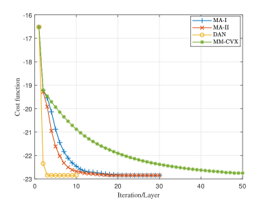
\bullet ‘MM-ADMM’: the optimization-based method proposed in Sec. III. A. To show the impact of 𝐓(k,l)superscript𝐓𝑘𝑙\mathbf{T}^{(k,l)} in MM-ADMM, we use two different 𝐓(k,l)superscript𝐓𝑘𝑙\mathbf{T}^{(k,l)}. Specifically, the first choice is 𝐓1(k,l)=tr(𝐇F(𝐮(k,l)))𝐈superscriptsubscript𝐓1𝑘𝑙trsubscript𝐇𝐹superscript𝐮𝑘𝑙𝐈\mathbf{T}_{1}^{(k,l)}=\mathrm{tr}(\mathbf{H}_{F}(\mathbf{u}^{(k,l)}))\mathbf{I}, and the second choice is 𝐓2(k,l)=λmax(𝐇F(𝐮(k,l)))𝐈superscriptsubscript𝐓2𝑘𝑙subscript𝜆subscript𝐇𝐹superscript𝐮𝑘𝑙𝐈\mathbf{T}_{2}^{(k,l)}=\lambda_{\max}(\mathbf{H}_{F}(\mathbf{u}^{(k,l)}))\mathbf{I}, which are denoted by ‘MA-I’ and ‘MA-II’, respectively. The parameters of MM-ADMM and MM-CVX are the same as that for DAN. The maximum number of MM iterations for MM-ADMM and MM-CVX is set as 303030 and 505050, respectively, unless specified otherwise.

2) Power allocation: We compare FP-WF with ‘CVX’, which represents the method for solving (45) by CVX.

IV-A Computational Cost

TABLE I: Running time in second for joint SN selection (ES, MA-I, MA-II, DAN) and power allocation (CVX, FP-WF) (Averaged Over 1000 Monte-Carlo trials)
Method ES MM-CVX MA-I MA-II DAN
CVX 18.6242 24.4350 10.0120 13.7984 6.6404
FP-WF 13.5733 19.4870 4.5109 9.1722 0.7724

Table I shows the running time222Configuration of this computer: CPU: Inter Core i9-9900 @3.10GHz; RAM: 16GB; Software: Python 3.10.9 in Microsoft visual studio code and Matlab 2020b. of the algorithms composed of different power allocation and SN selection methods. It can be observed that the running time of DAN &\& FP-WF is 0.7724 s, which is the lowest among all combinations. Meanwhile, we can observe that the running time of ES &\& CVX is 18.6242 s, which is about 24.11 times more than that of DAN &\& FP-WF. To further demonstrate the low computational complexity provided by DAN and FP-WF, we study the computational cost of the SN selection and power allocation methods, respectively.

TABLE II: Running time in second for SN selection (ES, MA-I, MA-II, DAN) (Averaged Over 1000 Monte-Carlo trials)
N𝑁N ES MM-CVX MA-I MA-II DAN
323232 4.2662 6.4081 1.3712 2.8322 0.2453
646464 34.7366 23.0416 3.9726 9.1618 0.3263
128128128 280.1406 93.2871 18.9184 40.0574 0.6316

Running time of the SN selection methods: Table II shows the running time of the SN selection algorithms with different N𝑁N. DAN achieves the lowest computational cost among the candidates with different N𝑁N. The computational consumption of ES is extremely large, especially when N𝑁N is large. For example, when N=128𝑁128N=128, the DAN is about 443 times faster than ES. MM-CVX is more time-consuming than MM-ADMM. Meanwhile, the running time of DAN is less than that of the MM-ADMM. There are two main reasons: 1) one layer of DAN has a lower computational cost than one iteration of MM-ADMM. In particular, DAN only requires the gradient, while MM-ADMM requires both the gradient and Hessian matrix, which needs more computational cost, and 2) owing to the well-trained 𝐓(k,l)superscript𝐓𝑘𝑙\mathbf{T}^{(k,l)}, DAN can converge faster than MM-ADMM, which will be shown in the following.

Convergence of the SN selection methods: The running time of MM-CVX, MM-ADMM and DAN is proportional to the required number of iterations/layers to converge. Fig. 3 shows the cost function over the number of the iterations (optimization-based methods) or the layers (DAN). First, MM-CVX needs about 50 iterations to converge, which is more than MM-ADMM and DAN. Meanwhile, we can observe that DAN can converge within 3 layers, while MM-ADMM needs about 15-20 iterations to converge, which leads to more running time. This is because, unlike MM-ADMM, DAN utilizes the momentum, which accumulates the gradient of the past layers and can thus speed up the convergence [37]. Meanwhile, we see that MM-ADMM-II can converge faster than MM-ADMM-I which indicates that the convergence of MM-ADMM highly depends on the choice of 𝐓(k,l)superscript𝐓𝑘𝑙\mathbf{T}^{(k,l)}. This is also the motivation to learn 𝐓(k,l)superscript𝐓𝑘𝑙\mathbf{T}^{(k,l)} in DAN.

Refer to caption
Figure 3: Cost function over the number of iterations/layers.

Running time of the power allocation methods: Table III shows the running time for the power allocation algorithms versus different Q𝑄Q. We can observe that the running time of FP-WF is much lower than CVX for different cases. This is because FP-WF is derived based on the Lagrange multiplier method, which can solve (45) more efficiently than the interior point method used by CVX.

TABLE III: Running time in second for power allocation (CVX, FP-WF) (Averaged Over 1000 Monte-Carlo trials)
Method Q=3𝑄3Q=3 Q=4𝑄4Q=4 Q=5𝑄5Q=5 Q=6𝑄6Q=6
CVX 1.7246 1.9854 2.0828 2.2966
FP-WF 0.0030 0.0060 0.0072 0.0087

IV-B Tracking Accuracy

The average root mean square error (RMSE) of multiple targets tracking over Q𝑄Q targets and K𝐾K frames is selected as the performance metric for multiple target tracking, which is defined as 1Q1Kq=1Qk=1K1Nmci=1Nmc𝐱q(k)𝐱^q(k,i)21𝑄1𝐾superscriptsubscript𝑞1𝑄superscriptsubscript𝑘1𝐾1subscript𝑁𝑚𝑐superscriptsubscript𝑖1subscript𝑁𝑚𝑐superscriptnormsuperscriptsubscript𝐱𝑞𝑘superscriptsubscript^𝐱𝑞𝑘𝑖2\frac{1}{Q}\frac{1}{K}\sum_{q=1}^{Q}\sum_{k=1}^{K}\sqrt{\frac{1}{N_{mc}}\sum_{i=1}^{N_{mc}}\|\mathbf{x}_{q}^{(k)}-\hat{\mathbf{x}}_{q}^{(k,i)}\|^{2}}, where 𝐱^q(k,i)superscriptsubscript^𝐱𝑞𝑘𝑖\hat{\mathbf{x}}_{q}^{(k,i)} denotes the estimated position of the target q𝑞q at the k𝑘kth time frame in the i𝑖ith Monte-Carlo trial, and Nmcsubscript𝑁𝑚𝑐N_{mc} denotes the number of Monte-Carlo trials. The number of tracking frames is set as K=10𝐾10K=10. Fig. 4 shows the average RMSE with different power budget P𝑃P. We have several observations. First, associated with different SN selection methods, FP-WF can achieve the same performance as CVX. Recalling from the results in Table III, compared to CVX, FP-WF can reduce the computational cost without losing performance loss. Second, we can observe that ES can achieve the best performance among the SN selection methods. However, from Table I, it can be observed that the running time of ES is extremely high, which limits its real application. Third, MM-CVX and MM-ADMM can achieve similar performance, but as shown in Table I, the computational cost of MM-CVX is higher than that of MM-ADMM. Furthermore, DAN can outperform MM-ADMM, which is because a more suitable 𝐓𝐓\mathbf{T} is learned by DAN. Finally, the performance of the nearest SN selection is worse than DAN. This is because the tracking performance is affected by both the distance and the angle from target to SNs. DAN takes both of them into consideration, while the nearest SN selection only considers the distance. This will be further demonstrated in the next part.
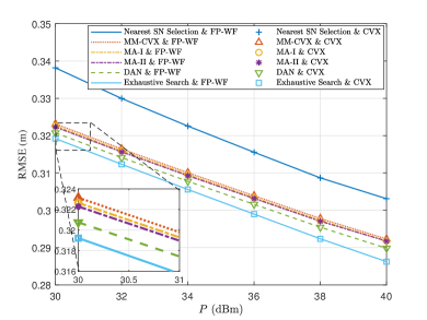
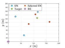
Refer to caption
Figure 4: Average RMSE versus the total power budget P𝑃P.
Refer to caption
(a)
Refer to caption
(b)
Refer to caption
(c)
Refer to caption
(d)
Figure 5: SN selection result by DAN at 4 consecutive frames. (a) Frame 2; (b) Frame 4; (c) Frame 6; (d) Frame 8;
Refer to caption
Figure 6: RMSE over tracking frames.

Illustration of SN selection: To better understand the effect of SN selection, we focus on the single target case in this section. The power allocated to the target is set as p=25𝑝25p=25 dBm. The initial state of the target is given by 𝐯=[10,0]T𝐯superscript100T\mathbf{v}=[-10,0]^{\mathrm{T}} m/s and 𝐱(0)=[124,124]Tsuperscript𝐱0superscript124124T\mathbf{x}^{(0)}=[124,124]^{\mathrm{T}} m. Fig. 5 shows the SN selection result by DAN in 4 consecutive frames. The selection depends on the geometric relation between the target and SNs. DAN does not always choose the nearest SNs, because, besides the distance, the different perspectives to observe the target provided by different SNs will also affect the tracking performance. Fig. 6 shows the corresponding RMSE over the tracking frames. It can be observed that DAN consistently outperforms the Nearest SN selection and achieves comparable performance as ES.

Effect of noise power:
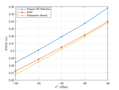
Refer to caption
Figure 7: RMSE versus different noise power σ2superscript𝜎2\sigma^{2}.

One of the biggest drawbacks of DL-based approaches is the performance degradation when the features (such as the noise power) in test data differ from those in training. This leads to the study of generalization in this part. Fig. 7 shows the performance under different noise power with N=32𝑁32N=32. When the noise power is different from that of the training data, DAN can provide a near-ES RMSE. It indicates that DAN can adapt to the change of σ2superscript𝜎2\sigma^{2}, which makes DAN attractive in real applications.

IV-C Accuracy-Complexity Tradeoff

By adjusting the termination tolerance and the maximum number of iterations, a tradeoff between computational cost and accuracy can be achieved by MM-ADMM. Meanwhile, the proposed DAN requires a fixed number of layers and thus has a fixed running time. Fig. 8 shows the RMSE performance of different algorithms versus the running time. It is observed that DAN can always outperform MM-ADMM in terms of both computational cost and RMSE. Moreover, though MM-ADMM-II can converge faster than MM-ADMM-I, 𝐓2(k,l)superscriptsubscript𝐓2𝑘𝑙\mathbf{T}_{2}^{(k,l)} requires more computational cost than 𝐓1(k,l)superscriptsubscript𝐓1𝑘𝑙\mathbf{T}_{1}^{(k,l)}. Thus, given the same time cost, MM-ADMM-I outperforms MM-ADMM-II.
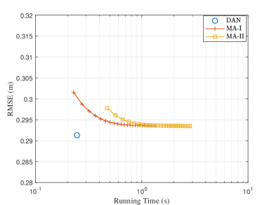
Refer to caption
Figure 8: NMSE versus the running time.

V Conclusion

In this paper, we considered the joint SN selection and power allocation problem for tracking multiple maneuvering targets in PMNs. To meet the stringent latency requirement of sensing applications, we proposed a model-driven approach for SN selection by unfolding the optimization-based MM-ADMM method. A novel DNN architecture was derived to speed up the convergence by exploiting the momentum, whose convergence property was also guaranteed by deriving the regret bound. Furthermore, we proposed an efficient power allocation method based on fixed-point water filling and revealed some physical insights. Simulation results demonstrated that the proposed method can achieve better performance than the existing methods with much lower computational cost. This work demonstrated that, by reducing the number of iterations and improving the effectiveness of each layer, model-driven approaches offer a promising solution to meet the stringent latency requirement of sensing applications.

Appendix A Proof of Theorem 1

Given (𝐮(k))superscript𝐮𝑘\mathcal{L}(\mathbf{u}^{(k)}) is convex, we have

𝒢(𝐮(k,l))𝒢(𝐮(k,))𝐝u(k,l),Δ𝐮(k,l),𝒢superscript𝐮𝑘𝑙𝒢superscript𝐮𝑘superscriptsubscript𝐝𝑢𝑘𝑙Δsuperscript𝐮𝑘𝑙\begin{split}\mathcal{G}(\mathbf{u}^{(k,l)})-\mathcal{G}(\mathbf{u}^{(k,\star)})\leq\left<\mathbf{d}_{u}^{(k,l)},\Delta\mathbf{u}^{(k,l)}\right>,\end{split} (50)

where Δ𝐮(k,l)=𝐮(k,l)𝐮(k,)Δsuperscript𝐮𝑘𝑙superscript𝐮𝑘𝑙superscript𝐮𝑘\Delta\mathbf{u}^{(k,l)}=\mathbf{u}^{(k,l)}-\mathbf{u}^{(k,\star)}. Since RLl=1L𝐝u(k,l),Δ𝐮(k,l)subscript𝑅𝐿superscriptsubscript𝑙1𝐿superscriptsubscript𝐝𝑢𝑘𝑙Δsuperscript𝐮𝑘𝑙R_{L}\leq\sum_{l=1}^{L}\left<\mathbf{d}_{u}^{(k,l)},\Delta\mathbf{u}^{(k,l)}\right>, the main idea of the proof is to find an upperbound of l=1L𝐝u(k,l),Δ𝐮(k,l)superscriptsubscript𝑙1𝐿superscriptsubscript𝐝𝑢𝑘𝑙Δsuperscript𝐮𝑘𝑙\sum_{l=1}^{L}\left<\mathbf{d}_{u}^{(k,l)},\Delta\mathbf{u}^{(k,l)}\right>. Recalling from (39), we have

𝚽l12Δ𝐮(k,l+1)2=𝚽l12(𝐮(k,l+1)𝐮(k,))2=(a)𝚽l12(𝐮(k,l)𝚽l1(𝐝(k,l)νl𝟏))𝐮(k,)2=(b)𝚽l12Δ𝐮(k,l)𝚽l12(𝐦^lρa,l𝐛^lνl𝟏)2=(c)𝚽l12Δ𝐮(k,l)22(1β1,l)𝐝u(k,l),Δ𝐮(k,l)2β1,l𝐦^l1ρa,l𝐛^lνl𝟏,Δ𝐮(k,l)+𝚽l12(𝐦^lρa,l𝐛^lνl𝟏)2,superscriptdelimited-∥∥superscriptsubscript𝚽𝑙12Δsuperscript𝐮𝑘𝑙12superscriptdelimited-∥∥superscriptsubscript𝚽𝑙12superscript𝐮𝑘𝑙1superscript𝐮𝑘2𝑎superscriptdelimited-∥∥superscriptsubscript𝚽𝑙12superscript𝐮𝑘𝑙superscriptsubscript𝚽𝑙1superscriptsubscript𝐝𝑘𝑙subscript𝜈𝑙1superscript𝐮𝑘2𝑏superscriptdelimited-∥∥superscriptsubscript𝚽𝑙12Δsuperscript𝐮𝑘𝑙superscriptsubscript𝚽𝑙12subscript^𝐦𝑙subscript𝜌𝑎𝑙subscript^𝐛𝑙subscript𝜈𝑙12𝑐superscriptdelimited-∥∥superscriptsubscript𝚽𝑙12Δsuperscript𝐮𝑘𝑙221subscript𝛽1𝑙superscriptsubscript𝐝𝑢𝑘𝑙Δsuperscript𝐮𝑘𝑙2subscript𝛽1𝑙subscript^𝐦𝑙1subscript𝜌𝑎𝑙subscript^𝐛𝑙subscript𝜈𝑙1Δsuperscript𝐮𝑘𝑙superscriptdelimited-∥∥superscriptsubscript𝚽𝑙12subscript^𝐦𝑙subscript𝜌𝑎𝑙subscript^𝐛𝑙subscript𝜈𝑙12\begin{split}&\|\mathbf{\Phi}_{l}^{\frac{1}{2}}\Delta\mathbf{u}^{(k,l+1)}\|^{2}=\|\mathbf{\Phi}_{l}^{\frac{1}{2}}(\mathbf{u}^{(k,l+1)}-\mathbf{u}^{(k,\star)})\|^{2}\\ &\overset{(a)}{=}\|\mathbf{\Phi}_{l}^{\frac{1}{2}}(\mathbf{u}^{(k,l)}-\mathbf{\Phi}_{l}^{-1}(\mathbf{d}_{\star}^{(k,l)}-\nu_{l}\mathbf{1}))-\mathbf{u}^{(k,\star)}\|^{2}\\ &\overset{(b)}{=}\|\mathbf{\Phi}_{l}^{\frac{1}{2}}\Delta\mathbf{u}^{(k,l)}-\mathbf{\Phi}_{l}^{-\frac{1}{2}}(\hat{\mathbf{m}}_{l}-\rho_{a,l}\hat{\mathbf{b}}_{l}-\nu_{l}\mathbf{1})\|^{2}\\ &\overset{(c)}{=}\left\|\mathbf{\Phi}_{l}^{\frac{1}{2}}\Delta\mathbf{u}^{(k,l)}\right\|^{2}-2\left<(1-\beta_{1,l})\mathbf{d}_{u}^{(k,l)},\Delta\mathbf{u}^{(k,l)}\right>\\ &\quad-2\left<\beta_{1,l}\hat{\mathbf{m}}_{l-1}-\rho_{a,l}\hat{\mathbf{b}}_{l}-\nu_{l}\mathbf{1},\Delta\mathbf{u}^{(k,l)}\right>\\ &\quad+\|\mathbf{\Phi}_{l}^{-\frac{1}{2}}(\hat{\mathbf{m}}_{l}-\rho_{a,l}\hat{\mathbf{b}}_{l}-\nu_{l}\mathbf{1})\|^{2},\end{split} (51)

where step (a) follows (39), step (b) follows (40), and step (c) follows (36).

By adding 2(1β1,l)𝐝u(k,l),Δ𝐮(k,l)𝚽l12Δ𝐮(k,l+1)221subscript𝛽1𝑙superscriptsubscript𝐝𝑢𝑘𝑙Δsuperscript𝐮𝑘𝑙superscriptnormsuperscriptsubscript𝚽𝑙12Δsuperscript𝐮𝑘𝑙122\left<(1-\beta_{1,l})\mathbf{d}_{u}^{(k,l)},\Delta\mathbf{u}^{(k,l)}\right>-\|\mathbf{\Phi}_{l}^{\frac{1}{2}}\Delta\mathbf{u}^{(k,l+1)}\|^{2} to both sides of (51), and dividing both sides of (51) by 2(1β1,l)21subscript𝛽1𝑙2(1-\beta_{1,l}), we have

𝐝u(k,l),Δ𝐮(k,l)=𝚽l12Δ𝐮(k,l)22(1β1,l)𝚽l12Δ𝐮(k,l+1)22(1β1,l)superscriptsubscript𝐝𝑢𝑘𝑙Δsuperscript𝐮𝑘𝑙superscriptnormsuperscriptsubscript𝚽𝑙12Δsuperscript𝐮𝑘𝑙221subscript𝛽1𝑙superscriptnormsuperscriptsubscript𝚽𝑙12Δsuperscript𝐮𝑘𝑙1221subscript𝛽1𝑙\displaystyle\left<\mathbf{d}_{u}^{(k,l)},\Delta\mathbf{u}^{(k,l)}\right>=\frac{\|\mathbf{\Phi}_{l}^{\frac{1}{2}}\Delta\mathbf{u}^{(k,l)}\|^{2}}{2(1-\beta_{1,l})}-\frac{\|\mathbf{\Phi}_{l}^{\frac{1}{2}}\Delta\mathbf{u}^{(k,l+1)}\|^{2}}{2(1-\beta_{1,l})}
=β1,l𝐦^l1,Δ𝐮(k,l)1β1,l+ρa,l𝐛^l,Δ𝐮(k,l)1β1,labsentsubscript𝛽1𝑙subscript^𝐦𝑙1Δsuperscript𝐮𝑘𝑙1subscript𝛽1𝑙subscript𝜌𝑎𝑙subscript^𝐛𝑙Δsuperscript𝐮𝑘𝑙1subscript𝛽1𝑙\displaystyle=-\frac{\left<\beta_{1,l}\hat{\mathbf{m}}_{l-1},\Delta\mathbf{u}^{(k,l)}\right>}{1-\beta_{1,l}}+\frac{\left<\rho_{a,l}\hat{\mathbf{b}}_{l},\Delta\mathbf{u}^{(k,l)}\right>}{1-\beta_{1,l}} (52)
+νl𝟏,Δ𝐮(k,l)1β1,l+𝚽l12(𝐦^lρa,l𝐛^lνl𝟏)22(1β1,l).subscript𝜈𝑙1Δsuperscript𝐮𝑘𝑙1subscript𝛽1𝑙superscriptnormsuperscriptsubscript𝚽𝑙12subscript^𝐦𝑙subscript𝜌𝑎𝑙subscript^𝐛𝑙subscript𝜈𝑙1221subscript𝛽1𝑙\displaystyle\quad+\frac{\left<\nu_{l}\mathbf{1},\Delta\mathbf{u}^{(k,l)}\right>}{1-\beta_{1,l}}+\frac{\|\mathbf{\Phi}_{l}^{-\frac{1}{2}}(\hat{\mathbf{m}}_{l}-\rho_{a,l}\hat{\mathbf{b}}_{l}-\nu_{l}\mathbf{1})\|^{2}}{2(1-\beta_{1,l})}.

By using the Young’s inequality for products, i.e., ±aba22+b22plus-or-minus𝑎𝑏superscript𝑎22superscript𝑏22\pm ab\leq\frac{a^{2}}{2}+\frac{b^{2}}{2}, the second, third, and fourth terms on the right-hand side of (52) are upperbounded by β1,l𝐦^l1,Δ𝐮(k,l)1β1,l𝚽l12𝐦^l122(1β1)+𝚽l12Δ𝐮(k,l)22(1β1)subscript𝛽1𝑙subscript^𝐦𝑙1Δsuperscript𝐮𝑘𝑙1subscript𝛽1𝑙superscriptnormsuperscriptsubscript𝚽𝑙12subscript^𝐦𝑙1221subscript𝛽1superscriptnormsuperscriptsubscript𝚽𝑙12Δsuperscript𝐮𝑘𝑙221subscript𝛽1-\frac{\left<\beta_{1,l}\hat{\mathbf{m}}_{l-1},\Delta\mathbf{u}^{(k,l)}\right>}{1-\beta_{1,l}}\leq\frac{\|\mathbf{\Phi}_{l}^{-\frac{1}{2}}\hat{\mathbf{m}}_{l-1}\|^{2}}{2(1-\beta_{1})}+\frac{\|\mathbf{\Phi}_{l}^{\frac{1}{2}}\Delta\mathbf{u}^{(k,l)}\|^{2}}{2(1-\beta_{1})}, 𝐛^l,Δ𝐮(k,l)1β1,l𝚽l12𝐛^l22(1β1)+𝚽l12Δ𝐮(k,l)22(1β1)subscript^𝐛𝑙Δsuperscript𝐮𝑘𝑙1subscript𝛽1𝑙superscriptnormsuperscriptsubscript𝚽𝑙12subscript^𝐛𝑙221subscript𝛽1superscriptnormsuperscriptsubscript𝚽𝑙12Δsuperscript𝐮𝑘𝑙221subscript𝛽1\frac{\left<\hat{\mathbf{b}}_{l},\Delta\mathbf{u}^{(k,l)}\right>}{1-\beta_{1,l}}\leq\frac{\|\mathbf{\Phi}_{l}^{-\frac{1}{2}}\hat{\mathbf{b}}_{l}\|^{2}}{2(1-\beta_{1})}+\frac{\|\mathbf{\Phi}_{l}^{\frac{1}{2}}\Delta\mathbf{u}^{(k,l)}\|^{2}}{2(1-\beta_{1})}, and 𝟏,Δ𝐮(k,l)1β1,l𝚽l12𝟏22(1β1)+𝚽l12Δ𝐮(k,l)22(1β1)1Δsuperscript𝐮𝑘𝑙1subscript𝛽1𝑙superscriptnormsuperscriptsubscript𝚽𝑙121221subscript𝛽1superscriptnormsuperscriptsubscript𝚽𝑙12Δsuperscript𝐮𝑘𝑙221subscript𝛽1\frac{\left<\mathbf{1},\Delta\mathbf{u}^{(k,l)}\right>}{1-\beta_{1,l}}\leq\frac{\|\mathbf{\Phi}_{l}^{-\frac{1}{2}}\mathbf{1}\|^{2}}{2(1-\beta_{1})}+\frac{\|\mathbf{\Phi}_{l}^{\frac{1}{2}}\Delta\mathbf{u}^{(k,l)}\|^{2}}{2(1-\beta_{1})}, respectively. By utilizing the inequality between the arithmetic mean and quadratic mean, the last term on the right-hand side of (52) is upperbounded by 𝚽l12(𝐦^lρa,l𝐛^lνl𝟏)22(1β1,l)3𝚽l12𝐦^l22(1β1)+3ρa,l2𝚽l12𝐛^l22(1β1)+3νl2𝚽l12𝟏22(1β1)superscriptnormsuperscriptsubscript𝚽𝑙12subscript^𝐦𝑙subscript𝜌𝑎𝑙subscript^𝐛𝑙subscript𝜈𝑙1221subscript𝛽1𝑙3superscriptnormsuperscriptsubscript𝚽𝑙12subscript^𝐦𝑙221subscript𝛽13superscriptsubscript𝜌𝑎𝑙2superscriptnormsuperscriptsubscript𝚽𝑙12subscript^𝐛𝑙221subscript𝛽13superscriptsubscript𝜈𝑙2superscriptnormsuperscriptsubscript𝚽𝑙121221subscript𝛽1\frac{\|\mathbf{\Phi}_{l}^{-\frac{1}{2}}(\hat{\mathbf{m}}_{l}-\rho_{a,l}\hat{\mathbf{b}}_{l}-\nu_{l}\mathbf{1})\|^{2}}{2(1-\beta_{1,l})}\leq\frac{3\|\mathbf{\Phi}_{l}^{-\frac{1}{2}}\hat{\mathbf{m}}_{l}\|^{2}}{2(1-\beta_{1})}+\frac{3\rho_{a,l}^{2}\|\mathbf{\Phi}_{l}^{-\frac{1}{2}}\hat{\mathbf{b}}_{l}\|^{2}}{2(1-\beta_{1})}+\frac{3\nu_{l}^{2}\|\mathbf{\Phi}_{l}^{-\frac{1}{2}}\mathbf{1}\|^{2}}{2(1-\beta_{1})}. Then, the upperbound of (52) can be given by

𝐝u(k,l),Δ𝐮(k,l)𝚽l12Δ𝐮(k,l)22(1β1,l)𝚽l12Δ𝐮(k,l+1)22(1β1,l)superscriptsubscript𝐝𝑢𝑘𝑙Δsuperscript𝐮𝑘𝑙subscriptsuperscriptnormsuperscriptsubscript𝚽𝑙12Δsuperscript𝐮𝑘𝑙221subscript𝛽1𝑙superscriptnormsuperscriptsubscript𝚽𝑙12Δsuperscript𝐮𝑘𝑙1221subscript𝛽1𝑙\displaystyle\left<\mathbf{d}_{u}^{(k,l)},\Delta\mathbf{u}^{(k,l)}\right>{\leq}\underbrace{\frac{\|\mathbf{\Phi}_{l}^{\frac{1}{2}}\Delta\mathbf{u}^{(k,l)}\|^{2}}{2(1-\beta_{1,l})}-\frac{\|\mathbf{\Phi}_{l}^{\frac{1}{2}}\Delta\mathbf{u}^{(k,l+1)}\|^{2}}{2(1-\beta_{1,l})}}_{\text{\char 172}}
+β1,l𝚽l12𝐦^l122(1β1)+ρa,l𝚽l12𝐛^l22(1β1)+νl𝚽l12𝟏22(1β1)subscriptsubscript𝛽1𝑙superscriptnormsuperscriptsubscript𝚽𝑙12subscript^𝐦𝑙1221subscript𝛽1subscriptsubscript𝜌𝑎𝑙superscriptnormsuperscriptsubscript𝚽𝑙12subscript^𝐛𝑙221subscript𝛽1subscriptsubscript𝜈𝑙superscriptnormsuperscriptsubscript𝚽𝑙121221subscript𝛽1\displaystyle+\underbrace{\frac{\beta_{1,l}\|\mathbf{\Phi}_{l}^{-\frac{1}{2}}\hat{\mathbf{m}}_{l-1}\|^{2}}{2(1-\beta_{1})}}_{\text{\char 173}}+\underbrace{\frac{\rho_{a,l}\|\mathbf{\Phi}_{l}^{-\frac{1}{2}}\hat{\mathbf{b}}_{l}\|^{2}}{2(1-\beta_{1})}}_{\text{\char 174}}+\underbrace{\frac{\nu_{l}\|\mathbf{\Phi}_{l}^{-\frac{1}{2}}\mathbf{1}\|^{2}}{2(1-\beta_{1})}}_{\text{\char 175}}
+β1,l𝚽l12Δ𝐮(k,l)22(1β1)+ρa,l𝚽l12Δ𝐮(k,l)22(1β1)+νl𝚽l12Δ𝐮(k,l)22(1β1)subscriptsubscript𝛽1𝑙superscriptnormsuperscriptsubscript𝚽𝑙12Δsuperscript𝐮𝑘𝑙221subscript𝛽1subscriptsubscript𝜌𝑎𝑙superscriptnormsuperscriptsubscript𝚽𝑙12Δsuperscript𝐮𝑘𝑙221subscript𝛽1subscriptsubscript𝜈𝑙superscriptnormsuperscriptsubscript𝚽𝑙12Δsuperscript𝐮𝑘𝑙221subscript𝛽1\displaystyle+\underbrace{\frac{\beta_{1,l}\|\mathbf{\Phi}_{l}^{\frac{1}{2}}\Delta\mathbf{u}^{(k,l)}\|^{2}}{2(1-\beta_{1})}}_{\text{\char 176}}+\underbrace{\frac{\rho_{a,l}\|\mathbf{\Phi}_{l}^{\frac{1}{2}}\Delta\mathbf{u}^{(k,l)}\|^{2}}{2(1-\beta_{1})}}_{\text{\char 177}}+\underbrace{\frac{\nu_{l}\|\mathbf{\Phi}_{l}^{\frac{1}{2}}\Delta\mathbf{u}^{(k,l)}\|^{2}}{2(1-\beta_{1})}}_{\text{\char 178}}
+3𝚽l12𝐦^l22(1β1)+3ρa,l2𝚽l12𝐛^l22(1β1)+3νl2𝚽l12𝟏22(1β1),subscript3superscriptnormsuperscriptsubscript𝚽𝑙12subscript^𝐦𝑙221subscript𝛽1subscript3superscriptsubscript𝜌𝑎𝑙2superscriptnormsuperscriptsubscript𝚽𝑙12subscript^𝐛𝑙221subscript𝛽1subscript3superscriptsubscript𝜈𝑙2superscriptnormsuperscriptsubscript𝚽𝑙121221subscript𝛽1\displaystyle+\underbrace{\frac{3\|\mathbf{\Phi}_{l}^{-\frac{1}{2}}\hat{\mathbf{m}}_{l}\|^{2}}{2(1-\beta_{1})}}_{\text{\char 179}}+\underbrace{\frac{3\rho_{a,l}^{2}\|\mathbf{\Phi}_{l}^{-\frac{1}{2}}\hat{\mathbf{b}}_{l}\|^{2}}{2(1-\beta_{1})}}_{\text{\char 180}}+\underbrace{\frac{3\nu_{l}^{2}\|\mathbf{\Phi}_{l}^{-\frac{1}{2}}\mathbf{1}\|^{2}}{2(1-\beta_{1})}}_{\text{\char 181}},

To bound RLsubscript𝑅𝐿R_{L}, we upperbound of the summation of the terms ①-⑩ over the index l𝑙l as follows.

A-1 Term ①

It can be shown that

𝚽l12Δ𝐮(k,l)2=i=1Nϕl,i1|Δui(k,l)|2=1α1,li=1N|v^l,i||Δui(k,l)|2+ρa,lΔ𝐮(k,l)2=(a)1α1,li=1Np=1l1β2β2lp2|du,i(k,p)||Δui(k,l)|2+ρa,lΔ𝐮(k,l)21β2α1(1β2)Du,1DΔl+DΔρaηal,superscriptdelimited-∥∥superscriptsubscript𝚽𝑙12Δsuperscript𝐮𝑘𝑙2superscriptsubscript𝑖1𝑁superscriptsubscriptitalic-ϕ𝑙𝑖1superscriptΔsuperscriptsubscript𝑢𝑖𝑘𝑙21subscript𝛼1𝑙superscriptsubscript𝑖1𝑁subscript^𝑣𝑙𝑖superscriptΔsuperscriptsubscript𝑢𝑖𝑘𝑙2subscript𝜌𝑎𝑙superscriptnormΔsuperscript𝐮𝑘𝑙2𝑎1subscript𝛼1𝑙superscriptsubscript𝑖1𝑁superscriptsubscript𝑝1𝑙1subscript𝛽2superscriptsubscript𝛽2𝑙𝑝2superscriptsubscript𝑑𝑢𝑖𝑘𝑝superscriptΔsuperscriptsubscript𝑢𝑖𝑘𝑙2subscript𝜌𝑎𝑙superscriptnormΔsuperscript𝐮𝑘𝑙21subscript𝛽2superscriptsubscript𝛼11subscript𝛽2subscript𝐷𝑢1subscript𝐷Δ𝑙subscript𝐷Δsubscript𝜌𝑎superscriptsubscript𝜂𝑎𝑙\begin{split}&\|\mathbf{\Phi}_{l}^{\frac{1}{2}}\Delta\mathbf{u}^{(k,l)}\|^{2}=\sum_{i=1}^{N}\phi_{l,i}^{-1}|\Delta u_{i}^{(k,l)}|^{2}\\ &=\frac{1}{\alpha_{1,l}}\sum_{i=1}^{N}\sqrt{|\hat{v}_{l,i}|}\cdot|\Delta u_{i}^{(k,l)}|^{2}+\rho_{a,l}||\Delta\mathbf{u}^{(k,l)}||^{2}\\ &\overset{(a)}{=}\frac{1}{\alpha_{1,l}}\sum_{i=1}^{N}\sum_{p=1}^{l}\sqrt{1-\beta_{2}}\beta_{2}^{\frac{l-p}{2}}|d_{u,i}^{(k,p)}|\cdot|\Delta u_{i}^{(k,l)}|^{2}\\ &\quad+\rho_{a,l}||\Delta\mathbf{u}^{(k,l)}||^{2}\\ &\leq\frac{\sqrt{1-\beta_{2}}}{\alpha_{1}^{-}(1-\sqrt{\beta_{2}})}D_{u,1}D_{\Delta}\sqrt{l}+D_{\Delta}\rho_{a}\eta_{a}^{l},\end{split} (53)

where step (a) comes from (38). Then, with the decreasing learning rate ϕl,i1superscriptsubscriptitalic-ϕ𝑙𝑖1\phi_{l,i}^{-1}, we have

l=1L(𝚽l12Δ𝐮(k,l)22(1β1,l)𝚽l12Δ𝐮(k,l+1)22(1β1,l))𝚽112Δ𝐮(k,1)22(1β1)+𝚽L12Δ𝐮(k,L+1)22(1β1)+l=2L(𝚽l12Δ𝐮(k,l)22(1β1,l)𝚽l112Δ𝐮(k,l)22(1β1,l))(a)1β2Du,1DΔα1(1β2)(1β1)L+ρaηaLDΔ1β1+1β2Du,1DΔα1(1β2)(1β1)+ρaηaDΔ1β1+l=2Li=1N(ϕl,iϕl1,i)|Δui(k,l)|22(1β1)(b)1β2Du,1DΔα1(1β2)(1β1)L+ρaηaDΔ1β1+1β2Du,1DΔα1(1β2)(1β1)+ρaηaDΔ1β1+DΔu,2Dϕ1β1,superscriptsubscript𝑙1𝐿superscriptnormsuperscriptsubscript𝚽𝑙12Δsuperscript𝐮𝑘𝑙221subscript𝛽1𝑙superscriptnormsuperscriptsubscript𝚽𝑙12Δsuperscript𝐮𝑘𝑙1221subscript𝛽1𝑙superscriptnormsuperscriptsubscript𝚽112Δsuperscript𝐮𝑘1221subscript𝛽1superscriptnormsuperscriptsubscript𝚽𝐿12Δsuperscript𝐮𝑘𝐿1221subscript𝛽1superscriptsubscript𝑙2𝐿superscriptnormsuperscriptsubscript𝚽𝑙12Δsuperscript𝐮𝑘𝑙221subscript𝛽1𝑙superscriptnormsuperscriptsubscript𝚽𝑙112Δsuperscript𝐮𝑘𝑙221subscript𝛽1𝑙𝑎1subscript𝛽2subscript𝐷𝑢1subscript𝐷Δsuperscriptsubscript𝛼11subscript𝛽21subscript𝛽1𝐿subscript𝜌𝑎superscriptsubscript𝜂𝑎𝐿subscript𝐷Δ1subscript𝛽11subscript𝛽2subscript𝐷𝑢1subscript𝐷Δsuperscriptsubscript𝛼11subscript𝛽21subscript𝛽1subscript𝜌𝑎subscript𝜂𝑎subscript𝐷Δ1subscript𝛽1superscriptsubscript𝑙2𝐿superscriptsubscript𝑖1𝑁subscriptitalic-ϕ𝑙𝑖subscriptitalic-ϕ𝑙1𝑖superscriptΔsuperscriptsubscript𝑢𝑖𝑘𝑙221subscript𝛽1𝑏1subscript𝛽2subscript𝐷𝑢1subscript𝐷Δsuperscriptsubscript𝛼11subscript𝛽21subscript𝛽1𝐿subscript𝜌𝑎subscript𝜂𝑎subscript𝐷Δ1subscript𝛽11subscript𝛽2subscript𝐷𝑢1subscript𝐷Δsuperscriptsubscript𝛼11subscript𝛽21subscript𝛽1subscript𝜌𝑎subscript𝜂𝑎subscript𝐷Δ1subscript𝛽1subscript𝐷subscriptΔ𝑢2subscript𝐷italic-ϕ1subscript𝛽1\begin{split}&\sum_{l=1}^{L}\left(\frac{\|\mathbf{\Phi}_{l}^{\frac{1}{2}}\Delta\mathbf{u}^{(k,l)}\|^{2}}{2(1-\beta_{1,l})}-\frac{\|\mathbf{\Phi}_{l}^{\frac{1}{2}}\Delta\mathbf{u}^{(k,l+1)}\|^{2}}{2(1-\beta_{1,l})}\right)\\ &\leq\frac{\|\mathbf{\Phi}_{1}^{\frac{1}{2}}\Delta\mathbf{u}^{(k,1)}\|^{2}}{2(1-\beta_{1})}+\frac{\|\mathbf{\Phi}_{L}^{\frac{1}{2}}\Delta\mathbf{u}^{(k,L+1)}\|^{2}}{2(1-\beta_{1})}\\ &\quad+\sum_{l=2}^{L}\left(\frac{\|\mathbf{\Phi}_{l}^{\frac{1}{2}}\Delta\mathbf{u}^{(k,l)}\|^{2}}{2(1-\beta_{1,l})}-\frac{\|\mathbf{\Phi}_{l-1}^{\frac{1}{2}}\Delta\mathbf{u}^{(k,l)}\|^{2}}{2(1-\beta_{1,l})}\right)\\ &\overset{(a)}{\leq}\frac{\sqrt{1-\beta_{2}}D_{u,1}D_{\Delta}}{\alpha_{1}^{-}(1-\sqrt{\beta_{2}})(1-\beta_{1})}\sqrt{L}+\frac{\rho_{a}\eta_{a}^{L}D_{\Delta}}{1-\beta_{1}}\\ &\quad+\frac{\sqrt{1-\beta_{2}}D_{u,1}D_{\Delta}}{\alpha_{1}^{-}(1-\sqrt{\beta_{2}})(1-\beta_{1})}+\frac{\rho_{a}\eta_{a}D_{\Delta}}{1-\beta_{1}}\\ &\quad+\frac{\sum\limits_{l=2}^{L}\sum\limits_{i=1}^{N}\left(\phi_{l,i}-\phi_{l-1,i}\right)|\Delta u_{i}^{(k,l)}|^{2}}{2(1-\beta_{1})}\\ &\overset{(b)}{\leq}\frac{\sqrt{1-\beta_{2}}D_{u,1}D_{\Delta}}{\alpha_{1}^{-}(1-\sqrt{\beta_{2}})(1-\beta_{1})}\sqrt{L}+\frac{\rho_{a}\eta_{a}D_{\Delta}}{1-\beta_{1}}\\ &\quad+\frac{\sqrt{1-\beta_{2}}D_{u,1}D_{\Delta}}{\alpha_{1}^{-}(1-\sqrt{\beta_{2}})(1-\beta_{1})}+\frac{\rho_{a}\eta_{a}D_{\Delta}}{1-\beta_{1}}+\frac{D_{\Delta_{u,2}}D_{\phi}}{1-\beta_{1}},\end{split} (54)

where step (a) follows (53) and step (b) follows

l=2Li=1N(ϕl,iϕl1,i)|Δui(k,l)|2DΔu,2i=1Nl=2L(ϕl,iϕl1,i)2DΔu,2Dϕ.superscriptsubscript𝑙2𝐿superscriptsubscript𝑖1𝑁subscriptitalic-ϕ𝑙𝑖subscriptitalic-ϕ𝑙1𝑖superscriptΔsuperscriptsubscript𝑢𝑖𝑘𝑙2subscript𝐷Δ𝑢2superscriptsubscript𝑖1𝑁superscriptsubscript𝑙2𝐿subscriptitalic-ϕ𝑙𝑖subscriptitalic-ϕ𝑙1𝑖2subscript𝐷subscriptΔ𝑢2subscript𝐷italic-ϕ\begin{split}&\sum\limits_{l=2}^{L}\sum\limits_{i=1}^{N}\left(\phi_{l,i}-\phi_{l-1,i}\right)|\Delta u_{i}^{(k,l)}|^{2}\\ &\leq D_{\Delta u,2}\sum\limits_{i=1}^{N}\sum\limits_{l=2}^{L}\left(\phi_{l,i}-\phi_{l-1,i}\right)\leq 2D_{\Delta_{u,2}}D_{\phi}.\end{split} (55)

A-2 Terms ② &\&

Since (1β1)1subscript𝛽1(1-\beta_{1}) is a non-zero constant, we focus on the upperbound of the terms l=1L𝚽l12𝐦^l2superscriptsubscript𝑙1𝐿superscriptnormsuperscriptsubscript𝚽𝑙12subscript^𝐦𝑙2\sum_{l=1}^{L}\|\mathbf{\Phi}_{l}^{-\frac{1}{2}}\hat{\mathbf{m}}_{l}\|^{2} and l=1Lβ1,l𝚽l12𝐦^l12superscriptsubscript𝑙1𝐿subscript𝛽1𝑙superscriptnormsuperscriptsubscript𝚽𝑙12subscript^𝐦𝑙12\sum_{l=1}^{L}\beta_{1,l}\|\mathbf{\Phi}_{l}^{-\frac{1}{2}}\hat{\mathbf{m}}_{l-1}\|^{2}. Denote m^l,isubscript^𝑚𝑙𝑖\hat{m}_{l,i} and du,isubscript𝑑𝑢𝑖d_{u,i} as the i𝑖ith entry of 𝐦^lsubscript^𝐦𝑙\hat{\mathbf{m}}_{l} and 𝐝u(k,l)superscriptsubscript𝐝𝑢𝑘𝑙\mathbf{d}_{u}^{(k,l)}, respectively. Then, we have

𝚽l12𝐦^l2=i=1Nm^l,i2ϕl,ii=1Nm^l,i2|v^l,i|/α1,l=i=1N(p=1l(1β1,p)q=1lpβ1,lq+1du,i(k,p))2|v^l,i|/α1,l(a)i=1Nα1,lη12l(p=1lβ1lp)(p=1lβ1lp(du,i(k,p))2)p=1l(1β2)β2lp|du,i(k,p)|2(b)α1,lη12l(1β1)1β2i=1N(p=1l(β1β2)lp|du,i(k,p)|),superscriptdelimited-∥∥superscriptsubscript𝚽𝑙12subscript^𝐦𝑙2superscriptsubscript𝑖1𝑁superscriptsubscript^𝑚𝑙𝑖2subscriptitalic-ϕ𝑙𝑖superscriptsubscript𝑖1𝑁superscriptsubscript^𝑚𝑙𝑖2subscript^𝑣𝑙𝑖subscript𝛼1𝑙superscriptsubscript𝑖1𝑁superscriptsuperscriptsubscript𝑝1𝑙1subscript𝛽1𝑝superscriptsubscriptproduct𝑞1𝑙𝑝subscript𝛽1𝑙𝑞1superscriptsubscript𝑑𝑢𝑖𝑘𝑝2subscript^𝑣𝑙𝑖subscript𝛼1𝑙𝑎superscriptsubscript𝑖1𝑁subscript𝛼1𝑙superscriptsubscript𝜂12𝑙superscriptsubscript𝑝1𝑙superscriptsubscript𝛽1𝑙𝑝superscriptsubscript𝑝1𝑙superscriptsubscript𝛽1𝑙𝑝superscriptsuperscriptsubscript𝑑𝑢𝑖𝑘𝑝2superscriptsubscript𝑝1𝑙1subscript𝛽2superscriptsubscript𝛽2𝑙𝑝superscriptsuperscriptsubscript𝑑𝑢𝑖𝑘𝑝2𝑏subscript𝛼1𝑙superscriptsubscript𝜂12𝑙1subscript𝛽11subscript𝛽2superscriptsubscript𝑖1𝑁superscriptsubscript𝑝1𝑙superscriptsubscript𝛽1subscript𝛽2𝑙𝑝superscriptsubscript𝑑𝑢𝑖𝑘𝑝\begin{split}&\|\mathbf{\Phi}_{l}^{-\frac{1}{2}}\hat{\mathbf{m}}_{l}\|^{2}=\sum_{i=1}^{N}\frac{\hat{m}_{l,i}^{2}}{\phi_{l,i}}\leq\sum_{i=1}^{N}\frac{\hat{m}_{l,i}^{2}}{\sqrt{|\hat{v}_{l,i}|}/\alpha_{1,l}}\\ &=\sum_{i=1}^{N}\frac{\left(\sum_{p=1}^{l}(1-\beta_{1,p})\prod_{q=1}^{l-p}\beta_{1,l-q+1}d_{u,i}^{(k,p)}\right)^{2}}{\sqrt{|\hat{v}_{l,i}|}/\alpha_{1,l}}\\ &\overset{(a)}{\leq}\sum_{i=1}^{N}\frac{\alpha_{1,l}\eta_{1}^{2l}\left(\sum_{p=1}^{l}\beta_{1}^{l-p}\right)\left(\sum_{p=1}^{l}\beta_{1}^{l-p}(d_{u,i}^{(k,p)})^{2}\right)}{\sqrt{\sum_{p=1}^{l}(1-\beta_{2})\beta_{2}^{l-p}|d_{u,i}^{(k,p)}|^{2}}}\\ &\overset{(b)}{\leq}\frac{\alpha_{1,l}\eta_{1}^{2l}}{(1-\beta_{1})\sqrt{1-\beta_{2}}}\sum_{i=1}^{N}\left(\sum_{p=1}^{l}\left(\frac{\beta_{1}}{\sqrt{\beta_{2}}}\right)^{l-p}|d_{u,i}^{(k,p)}|\right),\\ \end{split} (56)

where step (a) comes from the inequality (1β1,p)11subscript𝛽1𝑝1(1-\beta_{1,p})\leq 1, q=1lpβ1,lq+1β1lpη1lsuperscriptsubscriptproduct𝑞1𝑙𝑝subscript𝛽1𝑙𝑞1superscriptsubscript𝛽1𝑙𝑝superscriptsubscript𝜂1𝑙\prod_{q=1}^{l-p}\beta_{1,l-q+1}\leq\beta_{1}^{l-p}\eta_{1}^{l} and the Jensen inequality, i.e., (iaibiiai)2aibi2iaisuperscriptsubscript𝑖subscript𝑎𝑖subscript𝑏𝑖subscript𝑖subscript𝑎𝑖2subscript𝑎𝑖superscriptsubscript𝑏𝑖2subscript𝑖subscript𝑎𝑖\left(\frac{\sum_{i}a_{i}b_{i}}{\sum_{i}a_{i}}\right)^{2}\leq\frac{\sum a_{i}b_{i}^{2}}{\sum_{i}a_{i}}, and step (b) follows the inequalities p=1lβ1lp11β1superscriptsubscript𝑝1𝑙superscriptsubscript𝛽1𝑙𝑝11subscript𝛽1\sum_{p=1}^{l}\beta_{1}^{l-p}\leq\frac{1}{1-\beta_{1}} and p=1l(1β2)β2lp|du,i(k,p)|2(1β2)β2lp|du,i(k,p)|2superscriptsubscript𝑝1𝑙1subscript𝛽2superscriptsubscript𝛽2𝑙𝑝superscriptsuperscriptsubscript𝑑𝑢𝑖𝑘𝑝21subscript𝛽2superscriptsubscript𝛽2𝑙𝑝superscriptsuperscriptsubscript𝑑𝑢𝑖𝑘𝑝2\sum_{p=1}^{l}(1-\beta_{2})\beta_{2}^{l-p}|d_{u,i}^{(k,p)}|^{2}\geq(1-\beta_{2})\beta_{2}^{l-p}|d_{u,i}^{(k,p)}|^{2}.

By summing up (56) over the index l𝑙l, we have

l=1L𝚽l12𝐦^l2superscriptsubscript𝑙1𝐿superscriptnormsuperscriptsubscript𝚽𝑙12subscript^𝐦𝑙2\displaystyle\sum_{l=1}^{L}\|\mathbf{\Phi}_{l}^{-\frac{1}{2}}\hat{\mathbf{m}}_{l}\|^{2}
l=1Lα1,lη12l(1β1)1β2i=1N(p=1l(β1β2)lp|du,i(k,p)|)absentsuperscriptsubscript𝑙1𝐿subscript𝛼1𝑙superscriptsubscript𝜂12𝑙1subscript𝛽11subscript𝛽2superscriptsubscript𝑖1𝑁superscriptsubscript𝑝1𝑙superscriptsubscript𝛽1subscript𝛽2𝑙𝑝superscriptsubscript𝑑𝑢𝑖𝑘𝑝\displaystyle\leq\sum_{l=1}^{L}\frac{\alpha_{1,l}\eta_{1}^{2l}}{(1-\beta_{1})\sqrt{1-\beta_{2}}}\sum_{i=1}^{N}\left(\sum_{p=1}^{l}\left(\frac{\beta_{1}}{\sqrt{\beta_{2}}}\right)^{l-p}|d_{u,i}^{(k,p)}|\right)
=l=1Lα1,lη12l(1β1)1β2𝐝u(k,l)1(j=lL(β1β2)jl)absentsuperscriptsubscript𝑙1𝐿subscript𝛼1𝑙superscriptsubscript𝜂12𝑙1subscript𝛽11subscript𝛽2subscriptnormsuperscriptsubscript𝐝𝑢𝑘𝑙1superscriptsubscript𝑗𝑙𝐿superscriptsubscript𝛽1subscript𝛽2𝑗𝑙\displaystyle=\sum_{l=1}^{L}\frac{\alpha_{1,l}\eta_{1}^{2l}}{(1-\beta_{1})\sqrt{1-\beta_{2}}}||\mathbf{d}_{u}^{(k,l)}||_{1}\left(\sum_{j=l}^{L}\left(\frac{\beta_{1}}{\sqrt{\beta_{2}}}\right)^{j-l}\right) (57)
α1+Du,1(1β1)(1β1β2)1β2l=1Lη12llabsentsuperscriptsubscript𝛼1subscript𝐷𝑢11subscript𝛽11subscript𝛽1subscript𝛽21subscript𝛽2superscriptsubscript𝑙1𝐿superscriptsubscript𝜂12𝑙𝑙\displaystyle\leq\frac{\alpha_{1}^{+}D_{u,1}}{(1-\beta_{1})(1-\frac{\beta_{1}}{\sqrt{\beta_{2}}})\sqrt{1-\beta_{2}}}\sum_{l=1}^{L}\frac{\eta_{1}^{2l}}{\sqrt{l}}
(a)α1+Du,1(1β1)(1β1β2)1β2(1η12),𝑎superscriptsubscript𝛼1subscript𝐷𝑢11subscript𝛽11subscript𝛽1subscript𝛽21subscript𝛽21superscriptsubscript𝜂12\displaystyle\overset{(a)}{\leq}\frac{\alpha_{1}^{+}D_{u,1}}{(1-\beta_{1})(1-\frac{\beta_{1}}{\sqrt{\beta_{2}}})\sqrt{1-\beta_{2}}(1-\eta_{1}^{2})},

where we have utilized the property that l=1Lη12lll=1Lη12l11η12superscriptsubscript𝑙1𝐿superscriptsubscript𝜂12𝑙𝑙superscriptsubscript𝑙1𝐿superscriptsubscript𝜂12𝑙11superscriptsubscript𝜂12\sum_{l=1}^{L}\frac{\eta_{1}^{2l}}{\sqrt{l}}\leq\sum_{l=1}^{L}\eta_{1}^{2l}\leq\frac{1}{1-\eta_{1}^{2}} in step (a). Then, we have

l=1L𝚽l12𝐦^l2α1+Du,1(1β1)(1β1β2)1β2(1η12).superscriptsubscript𝑙1𝐿superscriptdelimited-∥∥superscriptsubscript𝚽𝑙12subscript^𝐦𝑙2superscriptsubscript𝛼1subscript𝐷𝑢11subscript𝛽11subscript𝛽1subscript𝛽21subscript𝛽21superscriptsubscript𝜂12\begin{split}&\sum_{l=1}^{L}\|\mathbf{\Phi}_{l}^{-\frac{1}{2}}\hat{\mathbf{m}}_{l}\|^{2}\leq\frac{\alpha_{1}^{+}D_{u,1}}{(1-\beta_{1})(1-\frac{\beta_{1}}{\sqrt{\beta_{2}}})\sqrt{1-\beta_{2}}(1-\eta_{1}^{2})}.\end{split}

Similarly, we can obtain

l=1Lβ1,l𝚽l12𝐦^l12l=1Lβ1,l𝚽l112𝐦^l12α1+β1Du,1(1β1)(1β1β2)1β2(1η12).superscriptsubscript𝑙1𝐿subscript𝛽1𝑙superscriptdelimited-∥∥superscriptsubscript𝚽𝑙12subscript^𝐦𝑙12superscriptsubscript𝑙1𝐿subscript𝛽1𝑙superscriptdelimited-∥∥superscriptsubscript𝚽𝑙112subscript^𝐦𝑙12superscriptsubscript𝛼1subscript𝛽1subscript𝐷𝑢11subscript𝛽11subscript𝛽1subscript𝛽21subscript𝛽21superscriptsubscript𝜂12\begin{split}&\sum_{l=1}^{L}\beta_{1,l}\|\mathbf{\Phi}_{l}^{-\frac{1}{2}}\hat{\mathbf{m}}_{l-1}\|^{2}\leq\sum_{l=1}^{L}\beta_{1,l}\|\mathbf{\Phi}_{l-1}^{-\frac{1}{2}}\hat{\mathbf{m}}_{l-1}\|^{2}\\ &\leq\frac{\alpha_{1}^{+}\beta_{1}D_{u,1}}{(1-\beta_{1})(1-\frac{\beta_{1}}{\sqrt{\beta_{2}}})\sqrt{1-\beta_{2}}(1-\eta_{1}^{2})}.\end{split} (58)

A-3 Terms ③ &\&

First, we have

l=1Lρa,l𝚽l12𝐛^l2l=1LρaηalDϕl𝐛^l2ρaDϕDb,21ηa,superscriptsubscript𝑙1𝐿subscript𝜌𝑎𝑙superscriptdelimited-∥∥superscriptsubscript𝚽𝑙12subscript^𝐛𝑙2superscriptsubscript𝑙1𝐿subscript𝜌𝑎superscriptsubscript𝜂𝑎𝑙superscriptsubscript𝐷italic-ϕ𝑙superscriptnormsubscript^𝐛𝑙2subscript𝜌𝑎subscript𝐷italic-ϕsubscript𝐷𝑏21subscript𝜂𝑎\begin{split}&\sum_{l=1}^{L}\rho_{a,l}\|\mathbf{\Phi}_{l}^{-\frac{1}{2}}\hat{\mathbf{b}}_{l}\|^{2}\leq\sum_{l=1}^{L}\rho_{a}\eta_{a}^{l}D_{\phi}^{l}||\hat{\mathbf{b}}_{l}||^{2}\leq\frac{\rho_{a}D_{\phi}D_{b,2}}{1-\eta_{a}},\end{split}

where Dϕl=maxiϕl,i1superscriptsubscript𝐷italic-ϕ𝑙subscript𝑖superscriptsubscriptitalic-ϕ𝑙𝑖1D_{\phi}^{l}=\max\limits_{i}\phi_{l,i}^{-1}. Similarly, we can obtain

l=1Lρa,l2𝚽l12𝐛^l2ρa2DϕDb,21ηa2.superscriptsubscript𝑙1𝐿superscriptsubscript𝜌𝑎𝑙2superscriptnormsuperscriptsubscript𝚽𝑙12subscript^𝐛𝑙2superscriptsubscript𝜌𝑎2subscript𝐷italic-ϕsubscript𝐷𝑏21superscriptsubscript𝜂𝑎2\sum_{l=1}^{L}\rho_{a,l}^{2}\|\mathbf{\Phi}_{l}^{-\frac{1}{2}}\hat{\mathbf{b}}_{l}\|^{2}\leq\frac{\rho_{a}^{2}D_{\phi}D_{b,2}}{1-\eta_{a}^{2}}. (59)

A-4 Terms ④ &\&

By the definition of νlsubscript𝜈𝑙\nu_{l} in (30), we have

νl𝐝(k,l)1𝐦^l1+ρa,l𝐛^l1.subscript𝜈𝑙subscriptnormsuperscriptsubscript𝐝𝑘𝑙1subscriptnormsubscript^𝐦𝑙1subscript𝜌𝑎𝑙subscriptnormsubscript^𝐛𝑙1\begin{split}\nu_{l}&\leq||\mathbf{d}_{\star}^{(k,l)}||_{1}\leq||\hat{\mathbf{m}}_{l}||_{1}+\rho_{a,l}||\hat{\mathbf{b}}_{l}||_{1}.\end{split} (60)

Similar to (56), we can obtain

l=1L𝐦^l1l=1Li=1N(p=1lq=1lpβ1,lq+1|du,i(k,p)|)l=1L𝐝u(k,p)1η1l(1β1)Du,1(1η1)(1β1).superscriptsubscript𝑙1𝐿subscriptnormsubscript^𝐦𝑙1superscriptsubscript𝑙1𝐿superscriptsubscript𝑖1𝑁superscriptsubscript𝑝1𝑙superscriptsubscriptproduct𝑞1𝑙𝑝subscript𝛽1𝑙𝑞1superscriptsubscript𝑑𝑢𝑖𝑘𝑝superscriptsubscript𝑙1𝐿subscriptnormsuperscriptsubscript𝐝𝑢𝑘𝑝1superscriptsubscript𝜂1𝑙1subscript𝛽1subscript𝐷𝑢11subscript𝜂11subscript𝛽1\begin{split}&\sum_{l=1}^{L}||\hat{\mathbf{m}}_{l}||_{1}\leq\sum_{l=1}^{L}\sum_{i=1}^{N}\left(\sum_{p=1}^{l}\prod_{q=1}^{l-p}\beta_{1,l-q+1}|d_{u,i}^{(k,p)}|\right)\\ &\leq\sum_{l=1}^{L}\frac{||\mathbf{d}_{u}^{(k,p)}||_{1}\eta_{1}^{l}}{(1-\beta_{1})}\leq\frac{D_{u,1}}{(1-\eta_{1})(1-\beta_{1})}.\end{split} (61)

Then, we have

l=1Lρa,l𝐛^l1=ρaDb,1l=1LηalρaDb,11ηa.superscriptsubscript𝑙1𝐿subscript𝜌𝑎𝑙subscriptnormsubscript^𝐛𝑙1subscript𝜌𝑎subscript𝐷𝑏1superscriptsubscript𝑙1𝐿superscriptsubscript𝜂𝑎𝑙subscript𝜌𝑎subscript𝐷𝑏11subscript𝜂𝑎\begin{split}&\sum_{l=1}^{L}\rho_{a,l}||\hat{\mathbf{b}}_{l}||_{1}=\rho_{a}D_{b,1}\sum_{l=1}^{L}\eta_{a}^{l}\leq\frac{\rho_{a}D_{b,1}}{1-\eta_{a}}.\\ \end{split} (62)

By substituting (61) and (62) into (64), we have

l=1Lνl𝚽l12𝟏2Dϕl=1LνlDϕ(Du,1(1η1)(1β1)+ρaDb,11ηa).\begin{split}&\sum_{l=1}^{L}\nu_{l}\|\mathbf{\Phi}_{l}^{-\frac{1}{2}}\mathbf{1}\|^{2}\leq D_{\phi}\sum_{l=1}^{L}\nu_{l}\\ &\quad\quad\leq D_{\phi}\left(\frac{D_{u,1}}{(1-\eta_{1})(1-\beta_{1})}+\frac{\rho_{a}D_{b,1}}{1-\eta_{a}}\right).\end{split} (63)

It thus follows that

l=1Lνl𝚽l12𝟏2Du,1Dϕ(1η1)(1β1)+ρaDb,1Dϕ1ηa.superscriptsubscript𝑙1𝐿subscript𝜈𝑙superscriptdelimited-∥∥superscriptsubscript𝚽𝑙1212subscript𝐷𝑢1subscript𝐷italic-ϕ1subscript𝜂11subscript𝛽1subscript𝜌𝑎subscript𝐷𝑏1subscript𝐷italic-ϕ1subscript𝜂𝑎\begin{split}&\sum_{l=1}^{L}\nu_{l}\|\mathbf{\Phi}_{l}^{-\frac{1}{2}}\mathbf{1}\|^{2}\leq\frac{D_{u,1}D_{\phi}}{(1-\eta_{1})(1-\beta_{1})}+\frac{\rho_{a}D_{b,1}D_{\phi}}{1-\eta_{a}}.\end{split} (64)

Similarly, we can obtain

l=1Lνl2𝚽l12𝟏22Du,12Dϕ(1η12)(1β1)2+2ρa2Db,12Dϕ(1ηa2).superscriptsubscript𝑙1𝐿superscriptsubscript𝜈𝑙2superscriptdelimited-∥∥superscriptsubscript𝚽𝑙12122superscriptsubscript𝐷𝑢12subscript𝐷italic-ϕ1superscriptsubscript𝜂12superscript1subscript𝛽122superscriptsubscript𝜌𝑎2superscriptsubscript𝐷𝑏12subscript𝐷italic-ϕ1superscriptsubscript𝜂𝑎2\begin{split}&\sum_{l=1}^{L}\nu_{l}^{2}\|\mathbf{\Phi}_{l}^{-\frac{1}{2}}\mathbf{1}\|^{2}\leq\frac{2D_{u,1}^{2}D_{\phi}}{(1-\eta_{1}^{2})(1-\beta_{1})^{2}}+\frac{2\rho_{a}^{2}D_{b,1}^{2}D_{\phi}}{(1-\eta_{a}^{2})}.\end{split}

A-5 Term ⑤

By (53), we have

l=1Lβ1,l𝚽l12Δ𝐮(k,l)2β11β2α1(1β2)Du,1DΔlη1l+DΔβ1ρaη1lηal(a)β11β2Du,1DΔα1(1β2)(1η1)2+β1ρaDΔ(1η1ηa),superscriptsubscript𝑙1𝐿subscript𝛽1𝑙superscriptdelimited-∥∥superscriptsubscript𝚽𝑙12Δsuperscript𝐮𝑘𝑙2subscript𝛽11subscript𝛽2superscriptsubscript𝛼11subscript𝛽2subscript𝐷𝑢1subscript𝐷Δ𝑙superscriptsubscript𝜂1𝑙subscript𝐷Δsubscript𝛽1subscript𝜌𝑎superscriptsubscript𝜂1𝑙superscriptsubscript𝜂𝑎𝑙𝑎subscript𝛽11subscript𝛽2subscript𝐷𝑢1subscript𝐷Δsuperscriptsubscript𝛼11subscript𝛽2superscript1subscript𝜂12subscript𝛽1subscript𝜌𝑎subscript𝐷Δ1subscript𝜂1subscript𝜂𝑎\begin{split}&\sum_{l=1}^{L}\beta_{1,l}\|\mathbf{\Phi}_{l}^{\frac{1}{2}}\Delta\mathbf{u}^{(k,l)}\|^{2}\\ &\leq\frac{\beta_{1}\sqrt{1-\beta_{2}}}{\alpha_{1}^{-}(1-\sqrt{\beta_{2}})}D_{u,1}D_{\Delta}\sqrt{l}\eta_{1}^{l}+D_{\Delta}\beta_{1}\rho_{a}\eta_{1}^{l}\eta_{a}^{l}\\ &\overset{(a)}{\leq}\frac{\beta_{1}\sqrt{1-\beta_{2}}D_{u,1}D_{\Delta}}{\alpha_{1}^{-}(1-\sqrt{\beta_{2}})(1-\eta_{1})^{2}}+\frac{\beta_{1}\rho_{a}D_{\Delta}}{(1-\eta_{1}\eta_{a})},\end{split} (65)

where we have utilized the bound of the arithmetic-geometric series, i.e., l=1Llη1l1(1η1)2superscriptsubscript𝑙1𝐿𝑙superscriptsubscript𝜂1𝑙1superscript1subscript𝜂12\sum_{l=1}^{L}l\eta_{1}^{l}\leq\frac{1}{(1-\eta_{1})^{2}} in (a).

A-6 Term ⑥

By replacing β1,lsubscript𝛽1𝑙\beta_{1,l} with ρa,lsubscript𝜌𝑎𝑙\rho_{a,l} in (LABEL:lemmabeta1l), we have

l=1Lρa,l𝚽l12Δ𝐮(k,l)2ρa1β2Du,1DΔα1(1β2)(1ηa)2+ρa2DΔ1ηa2.superscriptsubscript𝑙1𝐿subscript𝜌𝑎𝑙superscriptdelimited-∥∥superscriptsubscript𝚽𝑙12Δsuperscript𝐮𝑘𝑙2subscript𝜌𝑎1subscript𝛽2subscript𝐷𝑢1subscript𝐷Δsuperscriptsubscript𝛼11subscript𝛽2superscript1subscript𝜂𝑎2superscriptsubscript𝜌𝑎2subscript𝐷Δ1superscriptsubscript𝜂𝑎2\begin{split}&\sum_{l=1}^{L}\rho_{a,l}\|\mathbf{\Phi}_{l}^{\frac{1}{2}}\Delta\mathbf{u}^{(k,l)}\|^{2}\leq\frac{\rho_{a}\sqrt{1-\beta_{2}}D_{u,1}D_{\Delta}}{\alpha_{1}^{-}(1-\sqrt{\beta_{2}})(1-\eta_{a})^{2}}+\frac{\rho_{a}^{2}D_{\Delta}}{1-\eta_{a}^{2}}.\end{split}

A-7 Term ⑦

Recalling (61) and (62), we have

νl𝐦^l1+ρa,l𝐛^l1Du,1(1β1)η1l+ρaDb,1ηal.subscript𝜈𝑙subscriptnormsubscript^𝐦𝑙1subscript𝜌𝑎𝑙subscriptnormsubscript^𝐛𝑙1subscript𝐷𝑢11subscript𝛽1superscriptsubscript𝜂1𝑙subscript𝜌𝑎subscript𝐷𝑏1superscriptsubscript𝜂𝑎𝑙\begin{split}\nu_{l}&\leq||\hat{\mathbf{m}}_{l}||_{1}+\rho_{a,l}||\hat{\mathbf{b}}_{l}||_{1}\leq\frac{D_{u,1}}{(1-\beta_{1})}\eta_{1}^{l}+\rho_{a}D_{b,1}\eta_{a}^{l}.\end{split} (66)

Then, we can obtain

νl𝚽l12Δ𝐮(k,l)2=νli=1Nϕl,i|Δui(k,l)|2=νlα1,li=1N|v^l,i||Δui(k,l)|2+νlρa,lΔ𝐮(k,l)2νl1β2α1(1β2)Du,1DΔl+νlDΔρaηal.subscript𝜈𝑙superscriptdelimited-∥∥superscriptsubscript𝚽𝑙12Δsuperscript𝐮𝑘𝑙2subscript𝜈𝑙superscriptsubscript𝑖1𝑁subscriptitalic-ϕ𝑙𝑖superscriptΔsuperscriptsubscript𝑢𝑖𝑘𝑙2subscript𝜈𝑙subscript𝛼1𝑙superscriptsubscript𝑖1𝑁subscript^𝑣𝑙𝑖superscriptΔsuperscriptsubscript𝑢𝑖𝑘𝑙2subscript𝜈𝑙subscript𝜌𝑎𝑙superscriptnormΔsuperscript𝐮𝑘𝑙2subscript𝜈𝑙1subscript𝛽2superscriptsubscript𝛼11subscript𝛽2subscript𝐷𝑢1subscript𝐷Δ𝑙subscript𝜈𝑙subscript𝐷Δsubscript𝜌𝑎superscriptsubscript𝜂𝑎𝑙\begin{split}&\nu_{l}\|\mathbf{\Phi}_{l}^{\frac{1}{2}}\Delta\mathbf{u}^{(k,l)}\|^{2}=\nu_{l}\sum_{i=1}^{N}\phi_{l,i}|\Delta u_{i}^{(k,l)}|^{2}\\ &=\frac{\nu_{l}}{\alpha_{1,l}}\sum_{i=1}^{N}\sqrt{|\hat{v}_{l,i}|}\cdot|\Delta u_{i}^{(k,l)}|^{2}+\nu_{l}\rho_{a,l}||\Delta\mathbf{u}^{(k,l)}||^{2}\\ &\leq\frac{\nu_{l}\sqrt{1-\beta_{2}}}{\alpha_{1}^{-}(1-\sqrt{\beta_{2}})}D_{u,1}D_{\Delta}\sqrt{l}+\nu_{l}D_{\Delta}\rho_{a}\eta_{a}^{l}.\end{split} (67)

Similarly, we have

l=1Llνl=l=1Ll(Du,1(1β1)η1l+ρaDb,1ηal)Du,1(1β1)(1η1)2+ρaDb,1(1ηa)2,superscriptsubscript𝑙1𝐿𝑙subscript𝜈𝑙superscriptsubscript𝑙1𝐿𝑙subscript𝐷𝑢11subscript𝛽1superscriptsubscript𝜂1𝑙subscript𝜌𝑎subscript𝐷𝑏1superscriptsubscript𝜂𝑎𝑙subscript𝐷𝑢11subscript𝛽1superscript1subscript𝜂12subscript𝜌𝑎subscript𝐷𝑏1superscript1subscript𝜂𝑎2\begin{split}\sum_{l=1}^{L}\sqrt{l}\nu_{l}&=\sum_{l=1}^{L}\sqrt{l}\left(\frac{D_{u,1}}{(1-\beta_{1})}\eta_{1}^{l}+\rho_{a}D_{b,1}\eta_{a}^{l}\right)\\ &\leq\frac{D_{u,1}}{(1-\beta_{1})(1-\eta_{1})^{2}}+\frac{\rho_{a}D_{b,1}}{(1-\eta_{a})^{2}},\end{split} (68)
l=1Lηalνl=l=1Lηal(Du,1(1β1)η1l+ρaDb,1ηal)Du,1(1β1)(1η1)(1ηa)+ρaDb,1(1ηa)2.superscriptsubscript𝑙1𝐿superscriptsubscript𝜂𝑎𝑙subscript𝜈𝑙superscriptsubscript𝑙1𝐿superscriptsubscript𝜂𝑎𝑙subscript𝐷𝑢11subscript𝛽1superscriptsubscript𝜂1𝑙subscript𝜌𝑎subscript𝐷𝑏1superscriptsubscript𝜂𝑎𝑙subscript𝐷𝑢11subscript𝛽11subscript𝜂11subscript𝜂𝑎subscript𝜌𝑎subscript𝐷𝑏1superscript1subscript𝜂𝑎2\begin{split}\sum_{l=1}^{L}\eta_{a}^{l}\nu_{l}&=\sum_{l=1}^{L}\eta_{a}^{l}\left(\frac{D_{u,1}}{(1-\beta_{1})}\eta_{1}^{l}+\rho_{a}D_{b,1}\eta_{a}^{l}\right)\\ &\leq\frac{D_{u,1}}{(1-\beta_{1})(1-\eta_{1})(1-\eta_{a})}+\frac{\rho_{a}D_{b,1}}{(1-\eta_{a})^{2}}.\end{split} (69)

By substituting (68) and (69) into (67), we have

l=1Lνl𝚽l12Δ𝐮(k,l)2superscriptsubscript𝑙1𝐿subscript𝜈𝑙superscriptnormsuperscriptsubscript𝚽𝑙12Δsuperscript𝐮𝑘𝑙2\displaystyle\sum_{l=1}^{L}\nu_{l}\|\mathbf{\Phi}_{l}^{\frac{1}{2}}\Delta\mathbf{u}^{(k,l)}\|^{2}
(Du,1(1β1)(1η1)2+ρaDb,1(1ηa)2)1β2Du,1DΔα1(1β2)absentsubscript𝐷𝑢11subscript𝛽1superscript1subscript𝜂12subscript𝜌𝑎subscript𝐷𝑏1superscript1subscript𝜂𝑎21subscript𝛽2subscript𝐷𝑢1subscript𝐷Δsubscript𝛼11subscript𝛽2\displaystyle\leq\left(\frac{D_{u,1}}{(1-\beta_{1})(1-\eta_{1})^{2}}+\frac{\rho_{a}D_{b,1}}{(1-\eta_{a})^{2}}\right)\frac{\sqrt{1-\beta_{2}}D_{u,1}D_{\Delta}}{\alpha_{1}(1-\sqrt{\beta_{2}})}
+(Du,1(1β1)(1η1)(1ηa)+ρaDb,1(1ηa)2)DΔρa.subscript𝐷𝑢11subscript𝛽11subscript𝜂11subscript𝜂𝑎subscript𝜌𝑎subscript𝐷𝑏1superscript1subscript𝜂𝑎2subscript𝐷Δsubscript𝜌𝑎\displaystyle+\left(\frac{D_{u,1}}{(1-\beta_{1})(1-\eta_{1})(1-\eta_{a})}+\frac{\rho_{a}D_{b,1}}{(1-\eta_{a})^{2}}\right)D_{\Delta}\rho_{a}. (70)

By combining the upperbounds for the summations of terms -, (42) can be proved.

References

  • [1] F. Liu, C. Masouros, A. Li, H. Sun, and L. Hanzo, “Mu-mimo communications with mimo radar: From co-existence to joint transmission,” IEEE Trans. Wirel. Commun., vol. 17, no. 4, pp. 2755–2770, 2018.
  • [2] F. Liu, W. Yuan, C. Masouros, and J. Yuan, “Radar-assisted predictive beamforming for vehicular links: Communication served by sensing,” IEEE Trans. Wirel. Commun., vol. 19, no. 11, pp. 7704–7719, 2020.
  • [3] A. Zhang, M. L. Rahman, X. Huang, Y. J. Guo, S. Chen, and R. W. Heath, “Perceptive mobile networks: Cellular networks with radio vision via joint communication and radar sensing,” IEEE Veh. Technol. Mag., vol. 16, no. 2, pp. 20–30, 2021.
  • [4] L. Xie, P. Wang, S. Song, and K. B. Letaief, “Perceptive mobile network with distributed target monitoring terminals: Leaking communication energy for sensing,” IEEE Trans. Wirel. Commun., vol. 21, no. 12, pp. 10 193–10 207, 2022.
  • [5] L. Xie, S. Song, and K. B. Letaief, “Networked sensing with ai-empowered interference management: Exploiting macro-diversity and array gain in perceptive mobile networks,” arXiv preprint arXiv:2205.11331, 2022.
  • [6] L. Xie, S. Song, Y. C. Eldar, and K. B. Letaief, “Collaborative sensing in perceptive mobile networks: Opportunities and challenges,” IEEE Wirel. Commun., vol. 30, no. 1, pp. 16–23, 2023.
  • [7] E. Maşazade, R. Niu, P. K. Varshney, and M. Keskinoz, “Energy aware iterative source localization for wireless sensor networks,” IEEE Trans. Signal Process., vol. 58, no. 9, pp. 4824–4835, 2010.
  • [8] H. Chen, S. Ta, and B. Sun, “Cooperative game approach to power allocation for target tracking in distributed mimo radar sensor networks,” IEEE Sens. J., vol. 15, no. 10, pp. 5423–5432, 2015.
  • [9] J. Yan, W. Pu, S. Zhou, H. Liu, and M. S. Greco, “Optimal resource allocation for asynchronous multiple targets tracking in heterogeneous radar networks,” IEEE Trans. Signal Process., vol. 68, pp. 4055–4068, 2020.
  • [10] X. Shen and P. K. Varshney, “Sensor selection based on generalized information gain for target tracking in large sensor networks,” IEEE Trans. Signal Process., vol. 62, no. 2, pp. 363–375, 2013.
  • [11] W. Yi, Y. Yuan, R. Hoseinnezhad, and L. Kong, “Resource scheduling for distributed multi-target tracking in netted colocated mimo radar systems,” IEEE Trans. Signal Process., vol. 68, pp. 1602–1617, 2020.
  • [12] J. Yan, H. Liu, B. Jiu, B. Chen, Z. Liu, and Z. Bao, “Simultaneous multibeam resource allocation scheme for multiple target tracking,” IEEE Trans. Signal Process., vol. 63, no. 12, pp. 3110–3122, 2015.
  • [13] Y. Yuan, W. Yi, R. Hoseinnezhad, and P. K. Varshney, “Robust power allocation for resource-aware multi-target tracking with colocated mimo radars,” IEEE Trans. Signal Process., vol. 69, pp. 443–458, 2020.
  • [14] M. Xie, W. Yi, T. Kirubarajan, and L. Kong, “Joint node selection and power allocation strategy for multitarget tracking in decentralized radar networks,” IEEE Trans. Signal Process., vol. 66, no. 3, pp. 729–743, 2017.
  • [15] H. Sun, M. Li, L. Zuo, and P. Zhang, “Resource allocation for multitarget tracking and data reduction in radar network with sensor location uncertainty,” IEEE Trans. Signal Process., vol. 69, pp. 4843–4858, 2021.
  • [16] A. Das and D. Kempe, “Submodular meets spectral: Greedy algorithms for subset selection, sparse approximation and dictionary selection,” arXiv preprint arXiv:1102.3975, 2011.
  • [17] E. Elhamifar, G. Sapiro, and S. S. Sastry, “Dissimilarity-based sparse subset selection,” IEEE Trans. Pattern Anal. Mach. Intell., vol. 38, no. 11, pp. 2182–2197, 2015.
  • [18] M. Grant and S. Boyd, “Cvx: Matlab software for disciplined convex programming, version 2.1,” 2014.
  • [19] M. Borgerding, P. Schniter, and S. Rangan, “Amp-inspired deep networks for sparse linear inverse problems,” IEEE Trans. Signal Process., vol. 65, no. 16, pp. 4293–4308, 2017.
  • [20] B. Xin, Y. Wang, W. Gao, D. Wipf, and B. Wang, “Maximal sparsity with deep networks?” NeurIPS, vol. 29, 2016.
  • [21] Y. Yang, J. Sun, H. Li, and Z. Xu, “Admm-csnet: A deep learning approach for image compressive sensing,” IEEE Trans. Pattern Anal. Mach. Intell., vol. 42, no. 3, pp. 521–538, 2020.
  • [22] J. Johnston, Y. Li, M. Lops, and X. Wang, “Admm-net for communication interference removal in stepped-frequency radar,” IEEE Trans. Signal Process., vol. 69, pp. 2818–2832, 2021.
  • [23] S. Parkvall, E. Dahlman, A. Furuskar, and M. Frenne, “Nr: The new 5g radio access technology,” IEEE Communi. Stand. Mag., vol. 1, no. 4, pp. 24–30, 2017.
  • [24] C. Jauffret and Y. Bar-Shalom, “Track formation with bearing and frequency measurements in clutter,” IEEE Trans. Aerosp. Electron. Syst., vol. 26, no. 6, pp. 999–1010, 1990.
  • [25] E. Grossi, M. Lops, and L. Venturino, “Track-before-detect for multiframe detection with censored observations,” IEEE Trans. Aerosp. Electron. Syst., vol. 50, no. 3, pp. 2032–2046, 2014.
  • [26] L. Xie, Z. He, J. Tong, and W. Zhang, “A recursive angle-doppler channel selection method for reduced-dimension space-time adaptive processing,” IEEE Trans. Aerosp. Electron. Syst., vol. 56, no. 5, pp. 3985–4000, 2020.
  • [27] K. L. Bell, C. J. Baker, G. E. Smith, J. T. Johnson, and M. Rangaswamy, “Cognitive radar framework for target detection and tracking,” IEEE J. Sel. Top. Signal Process., vol. 9, no. 8, pp. 1427–1439, 2015.
  • [28] J. Helferty and D. Mudgett, “Optimal observer trajectories for bearings only tracking by minimizing the trace of the cramer-rao lower bound,” in Proc. 32th IEEE Conf. Decis. Control, 1993, pp. 936–939 vol.1.
  • [29] J. Helferty, D. Mudgett, and J. Dzielski, “Trajectory optimization for minimum range error in bearings-only source localization,” in Proceedings of OCEANS ’93, 1993, pp. II/229–II/234 vol.2.
  • [30] R. Bejar, B. Krishnamachari, C. Gomes, and B. Selman, “Distributed constraint satisfaction in a wireless sensor tracking system,” in Workshop on Distributed Constraint Reasoning, International Joint Conference on Artificial Intelligence, vol. 4, 2001.
  • [31] X. Zhai, Q. Shi, Y. Cai, and M. Zhao, “Joint transmit precoding and receive antenna selection for uplink multiuser massive mimo systems,” IEEE Trans. Commun., vol. 66, no. 11, pp. 5249–5260, 2018.
  • [32] M. Malek-Mohammadi, A. Koochakzadeh, M. Babaie-Zadeh, M. Jansson, and C. R. Rojas, “Successive concave sparsity approximation for compressed sensing,” IEEE Trans. Signal Process., vol. 64, no. 21, pp. 5657–5671, 2016.
  • [33] Y. Sun, P. Babu, and D. P. Palomar, “Majorization-minimization algorithms in signal processing, communications, and machine learning,” IEEE Trans. Signal Process., vol. 65, no. 3, pp. 794–816, 2016.
  • [34] S. Boyd, N. Parikh, E. Chu, B. Peleato, J. Eckstein et al., “Distributed optimization and statistical learning via the alternating direction method of multipliers,” Found. Trends® Mach. Learn., vol. 3, no. 1, pp. 1–122, 2011.
  • [35] L. Xie, Z. He, J. Tong, J. Li, and H. Li, “Transmitter polarization optimization for space-time adaptive processing with diversely polarized antenna array,” Signal Process., vol. 169, p. 107401, 2020.
  • [36] J. Bibby, “Axiomatisations of the average and a further generalisation of monotonic sequences,” Glas. Math. J., vol. 15, no. 1, p. 63–65, 1974.
  • [37] D. P. Kingma and J. Ba, “Adam: A method for stochastic optimization,” arXiv preprint arXiv:1412.6980, 2014.