Measuring Cause-Effect with the Variability of the Largest Eigenvalue

Abstract

We present a method to test and monitor structural relationships between time variables. The distribution of the first eigenvalue for lagged correlation matrices (Tracy-Widom distribution) is used to test structural time relationships between variables against the alternative hypothesis (Independence). This distribution studies the asymptotic dynamics of the largest eigenvalue as a function of the lag in lagged correlation matrices. By analyzing the time series of the standard deviation of the greatest eigenvalue for $2\times 2$ correlation matrices with different lags we can analyze deviations from the Tracy-Widom distribution to test structural relationships between these two time variables. These relationships can be related to causality. We use the standard deviation of the explanatory power of the first eigenvalue at different lags as a proxy for testing and monitoring structural causal relationships. The method is applied to analyse causal dependencies between daily monetary flows in a retail brokerage business allowing to control for liquidity risks.

1 Overview

The Marcenko-Pastur paper [1] on the spectrum of empirical correlation matrices turned out to be useful in many, very different contexts (neural networks, image processing, wireless communications, etc.). It became relevant in the last two decades, as a new statistical tool to analyse large dimensional data sets and can be used to try to identify common causes (or factors) that explain the dynamics of N quantities.

The realization of the $i^{th}$ quantity $(i=1,\dots,N)$ at “time” t $(t=1,\dots,T)$ will be denoted $r_{t}^{i}$, which are demeaned and standardized. The normalized $T\times N$ matrix of returns will be denoted as X: $X_{ti}=r^{t}_{i}/\sqrt{T}$. The Pearson estimator of the correlation matrix is given by:

$$E_{ij}=\frac{1}{T}\sum_{i=1}^{T}{r_{i}^{t}r_{j}^{t}\equiv\left(X^{T}X\right)_{ij}}$$ (1)

where $E$ will denote the empirical correlation matrix on a given realization, in contrast ti the true correlation matrix C of the underlying statistical process. The difference can be analysed by the Marcenko-Pastur result [1]. The empirical density of eigenvalues (the spectrum) is strongly distorted when compared to the ‘true’ density in the special asymptotic limit. When $T\rightarrow{\infty}$, $N\rightarrow{\infty}$, the spectrum has some degree of universality with respect to the distribution of the $r_{ti}$’s.

The lagged correlation matrix between past and future returns $\mathcal{C}_{ij}(\tau)$ can be defined as:

$$\mathcal{C}_{ij}(\tau)=\langle r_{i}^{t},r_{j}^{t+\tau}\rangle$$ (2)

such that $\mathcal{C}_{ij}(\tau=0)=\mathcal{C}_{ij}$ is the standard correlation coefficient. Whereas $\mathcal{C}_{ij}$ is clearly a symmetric matrix, $\mathcal{C}_{ij}(\tau>0)$ is in general non symmetric, and only obeys $\mathcal{C}_{ij}(\tau)$).

2 The Tracy-Widom Region

The Tracy-Widom result is that for a large class of $N\times N$ matrices (e.g. symmetric random matrices with i.i.d elements with a finite fourth moment, or empirical correlation matrices of i.i.d random variables with a finite fourth moment), the re-scaled distribution of $\lambda_{max}-\lambda^{\ast}$ converges towards the Tracy-Widom distribution, usually noted $F_{1}$:

$$Prob(\lambda_{max}\leq\lambda_{+}+\gamma N^{-2/3}u)=F_{1}(u)$$ (3)

where $\gamma$ is a constant that depends on the problem. Everything is known about the Tracy-Widom density $f_{1}(u)=F^{\prime}_{1}(u)$, in particular its left and right far tails:

$$\ln{f_{1}(u)\propto{-u}^{3/2},\ \ \ (u\rightarrow\infty)};\ \ \ln{f_{1}(u)\propto{-\left|u\right|}^{3},\ \ \ (u\rightarrow-\infty)}$$ (4)

The left tail is much thinner: pushing the largest eigenvalue inside the allowed band implies compressing the whole Coulomb-Dyson gas of charges, which is difficult. Using this analogy, the large deviation regime of the Tracy-Widom problem (i.e. for $\lambda_{max}-\lambda^{+}=O(1)$) can be obtained [2].

For square symmetric random matrices, the celebrated semicircle law of Wigner [3, 4] describes the limiting density of eigenvalues. There is an analog for covariance matrices [1], and independently, Stein [5]. The Marcenko-Pastur result is stated here for Wishart matrices with identity covariance $E=I$, but is true more generally, including non-null cases. Suppose that both $n$ and $p$ tend to $\infty$, in some ratio $n/p\rightarrow\gamma\geq 1$. Then the empirical distribution of the eigenvalues converges almost surely,

$$G_{p}(t)=\frac{1}{p}\#\left\{l_{i}:l_{i}\leq nt\right\}\rightarrow G(t)$$ (5)

and the limiting distribution has a density $g(t)=G^{\prime}(t)$:

$$g(t)=\frac{\gamma}{2\pi t}\sqrt{(b-t)(a-t)},\ \ a\leq t\ \leq b$$ (6)

where $a=(1-\gamma^{1/2})^{2}$ and $b=(1+\gamma^{1/2})^{2}$. Consider now the right-hand edge, and particularly the largest eigenvalue. Why the interest in extremes? In the estimation of a sparse mean vector, the maximum of n i.i.d. Gaussian noise variables plays a key role. Similarly, in distinguishing a ”signal subspace” of higher variance from many noise variables, one expects the largest eigenvalue of a null (or white) sample covariance matrix to play a basic role. The bulk limit (6) points to a strong law for the largest eigenvalue. Indeed, [6] shows that:

$$n^{-1}l_{1}\rightarrow(1+\gamma^{1/2})^{2},a.s$$ (7)

that is $l_{1}\sim(\sqrt{(}n)+\sqrt{(}p))^{2}$. Later Bai, Krishnaiah, Silverstein and Yin established that strong convergence occurred iff the parent distribution had zero mean and finite fourth moment. For more details, full citations and results on the smallest eigenvalue [7]. However, these results say nothing about the variability of the largest eigenvalue, let alone about its distribution. For a survey of existing results [8]. For example, [[9], page 1284] gives an exact expression in terms of a zonal polynomial series for a confluent hypergeometric function of matrix argument:

$$P(l_{1}\leq nt)=d_{p,n}t^{pn/2}_{1}F_{1}(1/2n;1/2(n+p+1);-1/2bt\mathcal{I}_{p}))$$ (8)

where $d_{p,n}$ is a constant depending only on p and n [cf. also [8], page 421]. There are explicit evaluations for p = 2, 3, but in general the alternating series converges very slowly, even for small n and p, and so is difficult to use in practice. For fixed p and large n, the classic paper by [10] gives the limiting joint distribution of the roots, but the marginal distribution of $l_{1}$ is hard to extract even in the null case $X=I$. [11] gives a series approximation again for p = 2, 3. In general, there are upper bounds on the d.f. using p independent $\chi^{2}(n)$. Overall, there is little that helps numerically with approximations for large p. We now turn to what can be derived from random matrix theory (RMT) methods. Suppose that $X=(X_{jk})_{n\times p}$ has entries which are i.i.d. $X_{jk}\sim N(0,1)$. Denote the sample eigenvalues of the Wishart matrix $X^{\prime}X$ by $l_{1}>\dots>l_{p}$. Define center and scaling constants:

$$\mu_{np}=(\sqrt{n-1}+\sqrt{p})^{2}$$ (9)

$$\sigma_{np}=(\sqrt{n-1}+\sqrt{p})(\frac{1}{\sqrt{n-1}}+\frac{1}{\sqrt{p}})^{1/3}$$ (10)

The Thacy-Widom law of order 1 has distribution function defined by:

$$F_{1}(s)=\exp\left\{-\frac{1}{2}\int_{s}^{\infty}{q(x)+(x-s)q^{2}(x)dx}\right\},s\in\mathbb{R}$$ (11)

where q solves the (nonlinear) Painleve II differential equation:

$$\begin{split}q^{\prime\prime}(x)=xq(x)+2q^{3}(x)\\ q(x)\sim A_{i}(x)\ \ as\ \ x\rightarrow+\infty\end{split}$$ (12)

and $A_{i}(x)$ denotes the Airy function. This distribution was found by Tracy and Widom (1996) as the limiting law of the largest eigenvalue of an n by n Gaussian symmetric matrix.

Theorem 2.1.

Let $\mathcal{W}$ be a white Wishart matrixand $l_{1}$ be its largets eigenvalue. Then:

$$\frac{l_{1}-\mu_{np}}{\sigma_{np}}\overset{\mathcal{D}}{\longrightarrow}W_{1}\sim F_{1}$$ (13)

where the center and scaling constants are:

$$\mu_{np}=\left(\sqrt{n-1}+\sqrt{p}\right)^{2}\ ,\ \sigma_{np}=\mu_{np}\left(\left(n-1\right)^{-1/2}+p^{-1/2}\right)^{1/3}$$ (14)

and $F_{1}$ stands for the distribution function of the Tracy-Widom law of order 1.

The theorem is stated for situations in which $n>p$. However, it applies equally well if $n<p$ are both large, simply by reversing the roles of n and p in (9) and (10). The limiting distribution function $F_{1}$ is a particular distribution from a family of distributions $F_{\beta}$. For $\beta=1,2,4$ functions $F_{\beta}$ appear as the limiting distributions for the largest eigenvalues in the ensembles GOE, GUE and GSE, correspondingly. For the largest eigenvalue $l_{\max}(\mathcal{A})$ of the random matrix $\mathcal{A}$ (GOE $(\beta=1)$, GUE $(\beta=2)$ or GSE $(\beta=4)$) its distribution function $F_{N,\beta}(s)=P(l_{\max}(\mathcal{A})<s)$, $\beta=1,2,4$ satisfies the limit law in (8) with $l_{1}=l_{\max}(\mathcal{A})$, and $F_{1}=F_{\beta}$ given by (11).

From (12), the Airy special function $A_{i}(s)$ is one of the pairs of linearly independent solutions to the differential equation: $w^{\prime\prime}-zw=0$ such that:

$$\lim_{s\rightarrow\infty}{\frac{q(s)}{A_{i}(s)}=1}$$ (15)

The Painleve II is a second-order ordinary differential equation of the form $\frac{d^{2}w}{dz^{2}}=F(z,w,dw/dz)$. In Figure 1 [12], we can see some simulations for square cases $n-p=5,10$ and $100$, using $R=10,000$ replications (s is the lag value).

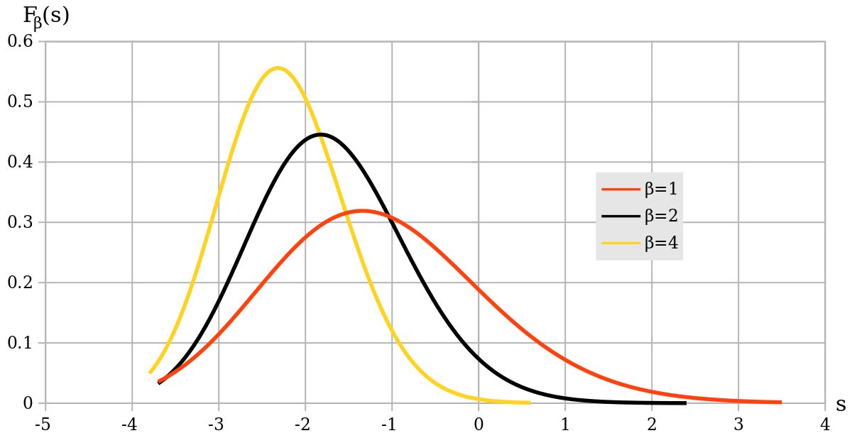
Figure 1: The Tracy-Widom distribution [12]

The main conclusion is that the Tracy-Widom distribution $F_{1}$ provides a usable numerical approximation to the null distribution of the largest principal component from Gaussian data even for quite moderate values of n and p. In particular, we have the following simple approximate rules of thumb:

• About $83\%$ of the distribution is less than $\mu_{np}=(\sqrt{n-1}+\sqrt{p})^{2}$

• About $95\%$ and $99\%$ lie below $\mu_{np}+\sigma_{np}$ and $\mu_{np}+2\sigma_{np}$ respectively

3 Method

We can monitor the empirical value of $\sigma_{np}$ in time from data. However, our method focuses on $\sigma_{\lambda}$, the standard deviation of the explanatory power for the first eigenvalue in $2\times 2$ matrices, $\frac{\lambda_{1}}{\lambda_{1}+\lambda_{2}}$, instead of just $\lambda_{1}-\lambda_{2}$ as with $\sigma_{np}$. This allows us to deal with a measure with empirical sense for the method. With extreme values of $\sigma_{\lambda}$ indicating deviations from the Tracy-Widom distribution $F_{1}$ which implies asymptotically independence versus structural time (causal) relationships. In Algorithm 1 we present the method for any dataset.

Data: Set of M causal variables candidates $X\in\mathbb{R}^{M}$, effect variable candidate $Y\in\mathbb{R}$, window $w$ for correlations, and $\max lag$ for the maximum lag for the Tracy-Widom distribution

Result: For each causal candidate variable, series $\sigma_{\lambda}[0,\dots,N]$.

for $0\leq k\leq N$ do

       $X=X[k-w\colon k,\colon]$;   $X=(X-mean(X))/std(X)$

       $Y=Y[k-w\colon k,\colon]$;   $Y=(Y-mean(Y))/std(Y)$

       for $1\leq j\leq M$ do

             for $0\leq i\leq\max lag$ do

                   $X[\colon,j]=X[\colon,j].shift(period=i)$

                   $X^{\prime}[j]=[Y[\colon],X[\colon,j]]^{T}$

                   $PCA[j]=PCA(X^{\prime}[j])$

                   $V[j,i]=\frac{\lambda_{1}}{\lambda_{1}+\lambda_{2}}$

                  

             end for

            $\sigma_{\lambda}[k,j]=std(V[1,\dots,\max lag;j])$

            

       end for

      

end for

Algorithm 1 Structural time dependence indicator ($\sigma_{\lambda}$)

In Figure 2, we show the average of the $\sigma_{\lambda}$ for 10 i.i.d time series generated from a Normal distribution. For this, Algorithm 1 is applied to sets of 2 different time-series. In Figure 3, we compare the average values of $\sigma_{\lambda}$ for the i.i.d series from the previous case with the average values for Algorithm 1 applied to time series variables from a financial dataset. The hypothesis can be simply verified from data as for independent time series the values of the indicator $\sigma_{\lambda}$ are much smaller than the values for time series with structural relationships.

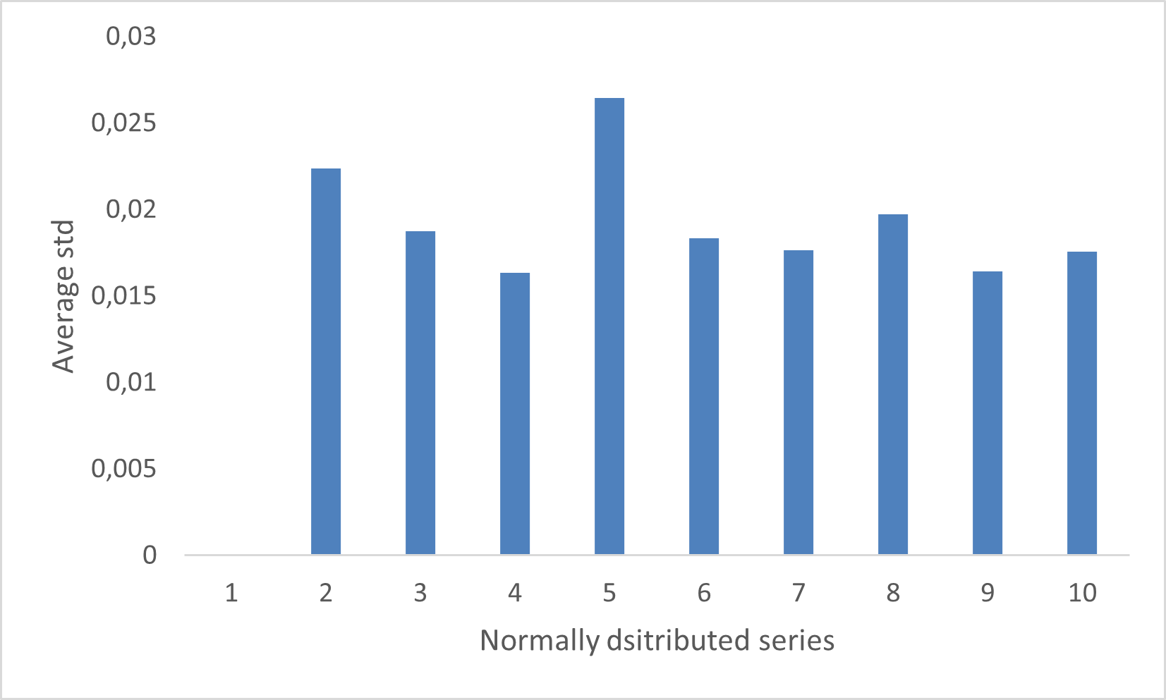
Figure 2: Average of $\sigma_{\lambda}$ for different lags for 10 i.i.d time series generated from a Normal distribution (400 time stamps)

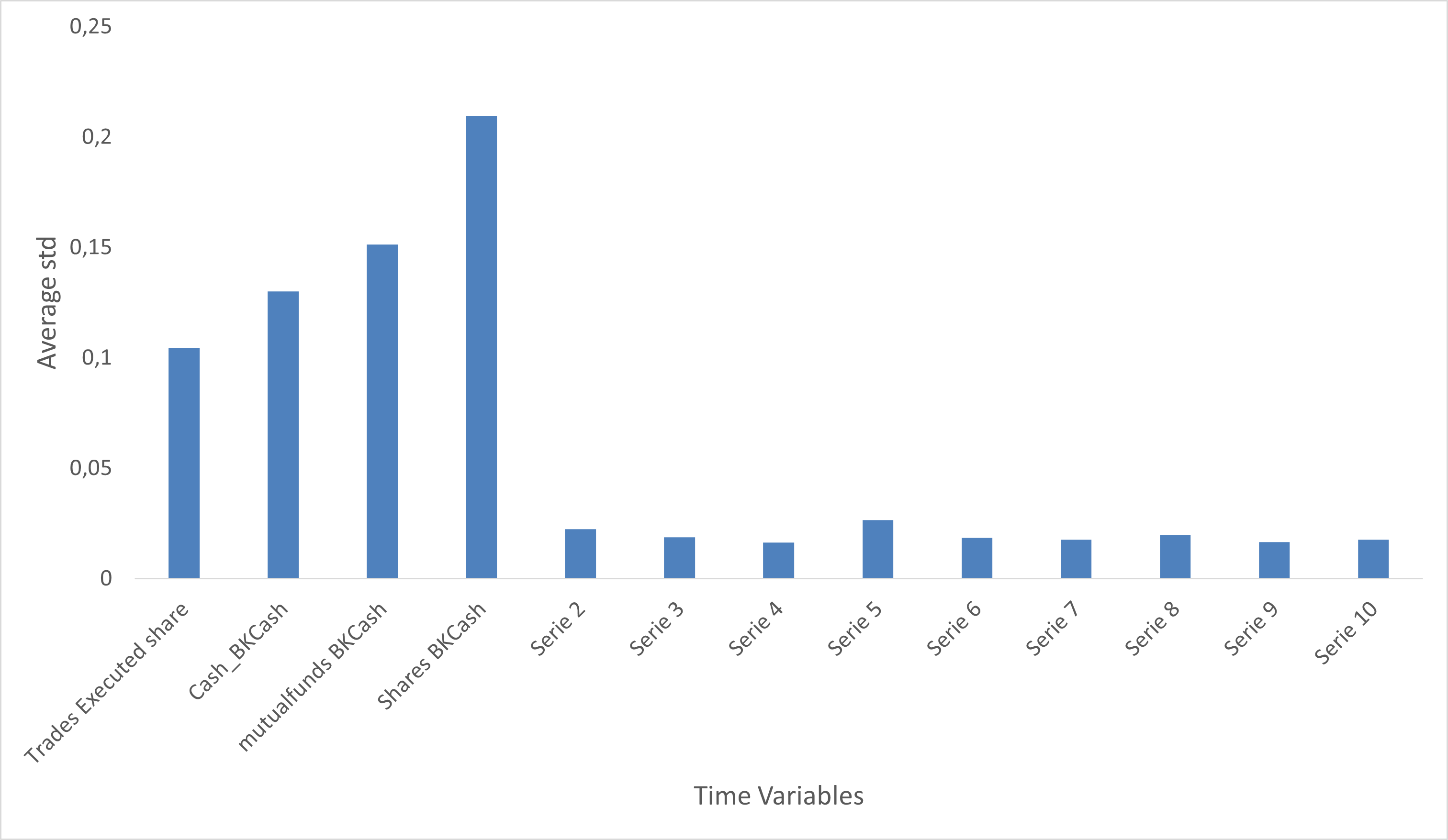
Figure 3: Average of $\sigma_{\lambda}$ for different lags. Causal candidates variables with greatest average $\sigma_{\lambda}$ vs i.i.d variables cases from Normal distribution (400 time stamps sample)

4 Experiments

For the experiments, we analyse daily brokerage activities with time series data of 15000 clients approximately. Our goal is to analyse the power of the structural temporal (causal) relationship between cash balance and other variables in time. Experiments are performed in cause-effect pairs with effect being cash balance, but for illustration we plot the results in thematic buckets. The buckets are:

• The account status includes the daily amount in account currency of open positions in different products including Shares, Bonds, Mutual Funds, CFDs, Derivatives, FX Spot and ETO.

• Bookkeeping cash includes all the daily cash movements in the account currency, both internal and external cash transactions, including the financial product that is the subject of the transaction.

• Trades Executes is focused in the daily buying and selling transaction activities in the account currency for all clients in all broker products.

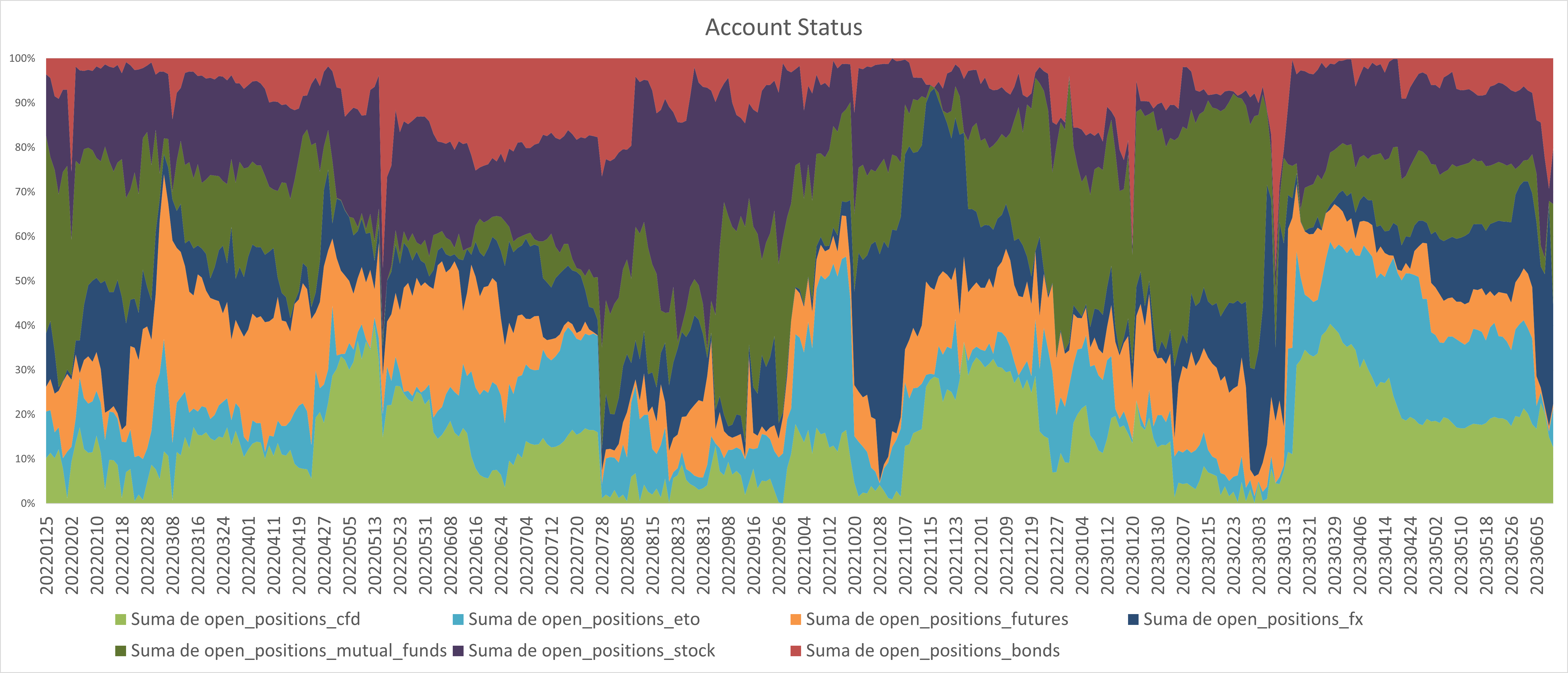
Figure 4: Account Status, value of $\sigma_{\lambda}$ for lag 2, cash balance vs broker securities open positions

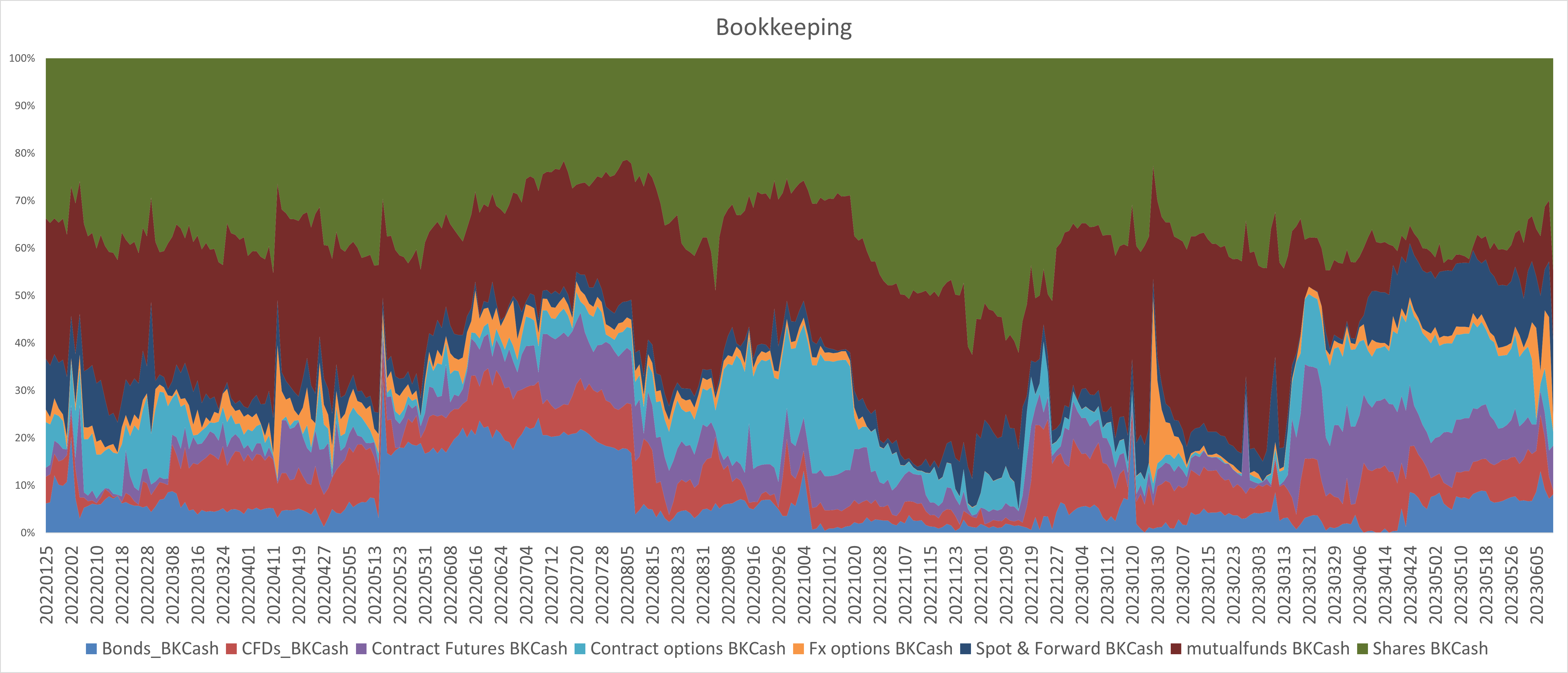
Figure 5: Bookkeeping cash, value of $\sigma_{\lambda}$ for lag 2, cash balance vs broker trading transactions

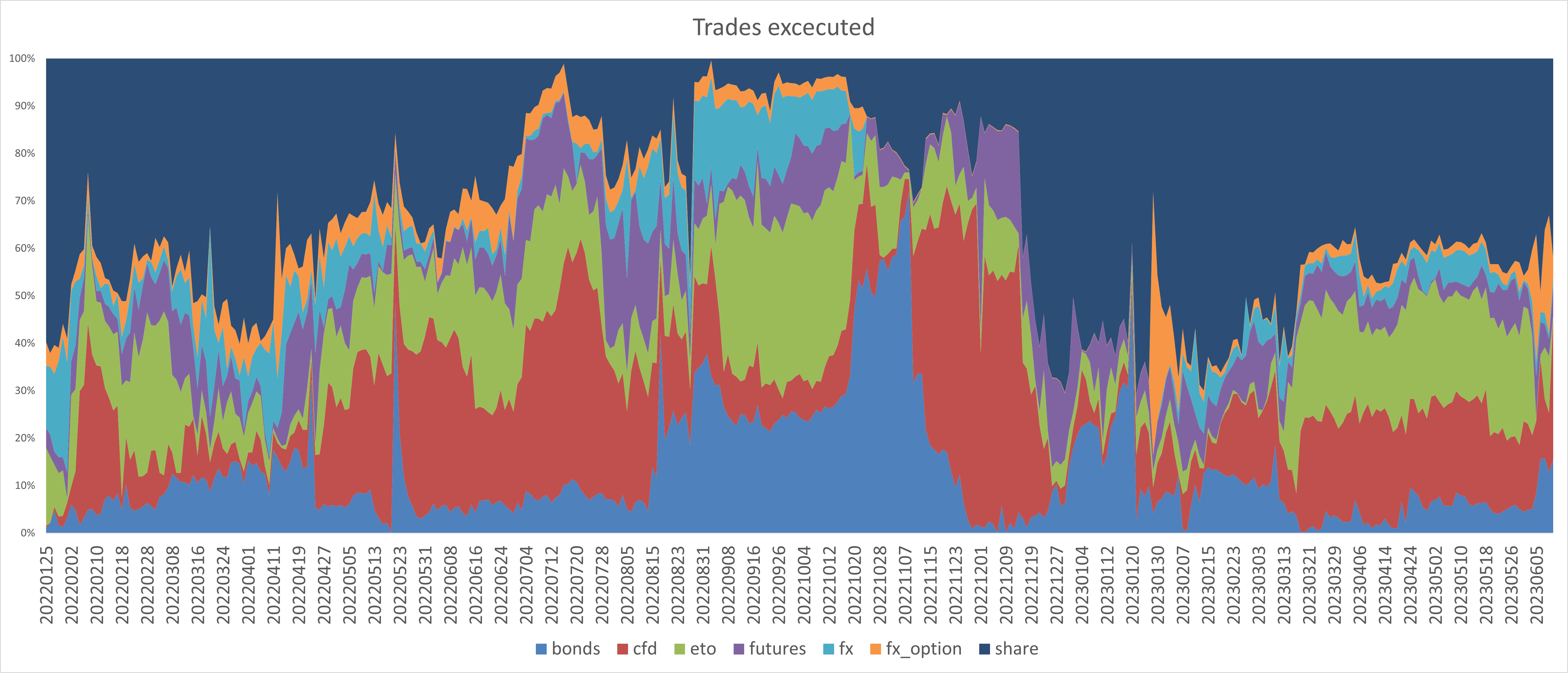
Figure 6: Broker trades executed vs cash balance, value of $\sigma_{\lambda}$ for lag 2

• From experiments we can see that account status bucket has more mixed results, with Mutual Funds from November 2022 until March 2023 holding majority. After that, the majority of cash movements could be explained by Stocks (Shares) (Figure 4).

• In the Bookkeeping cash bucket we see a defined pattern of the majority of cash transactions coming from shares activities. Until March 2023 this majority was shared with Mutual Funds however, this stopped from march on-wards and taking some importance the derivatives and FX products since March. The relationship is studied with respect to daily variations of cash balance gross amount (net outflows plus inflows) and not the total amount of flows (Figure 5).

• Finally, the trades executed bucket shows very similar behaviour than the Bookkeeping cash serving as validation point for our results (Figure 6). The reason why Mutual Funds are not in this picture is because the execution process is different for Mutual Funds, much of operations not having to be converted to cash. This could mean that, although Mutual Funds has been a product that at least historically until March 2023 has been responsible for the movement of cash balance of our clients (seen Bookkeeping), this has not been due to daily executions in funds from cash but in the form of internal and external transfer funds. With regards to trades executed, we can see that from June 2022 until December 2022 the relationships where mixed with shares not holding the majority. From December 2022 until now shares have hold the majority with some derivatives gaining importance since march.

In Figure 7, we show the average $\sigma_{\lambda}$ for lags 2 and 5 of the top candidates with greater values in the sample dataset (causal candidates). We perform the Granger causality test [13] with the sample dataset to compare results with our method. In Figures 8 and 9, we show the values for the logarithm of the inverse of the p-value for the Granger causality test for lags 2 and 5 respectively. We can see discrepancies between the Granger Causality test and our method, however our method is closer to the structural causal relationship based on empirical evidence from the dataset. In the case of the Granger test, the CFD product seems to be the one most causally related with the cash balance, in contrast to the product shares or stocks for our method. The issue with the Granger causality test is that is window based, which means that it depends on the sample time interval you choose without a dynamic sense of the causal relationships. On the other hand, a big structural relationship in one data point out of the full sample can bias the results. In contrast, our method is rolling window based, which means that is adaptive and able to capture changes in causal or structural relationships. It is less biased to causal point relationships focusing more on persistent dynamics. The CFDs business is highly correlated with the equity business, reason why the Granger causal test chooses CFDs against our method choosing Shares or stocks. However, our method is able to infer causality better in that, the Shares business is the biggest in size and flows and the CFDs business is much smaller. To measure true causal relationships between these flows, the time series and correlations are not necessary as the flow size matters, and our method is able to capture causality better, as it avoids window biases coming from extreme point values which are more related to correlation than to causal dynamics.

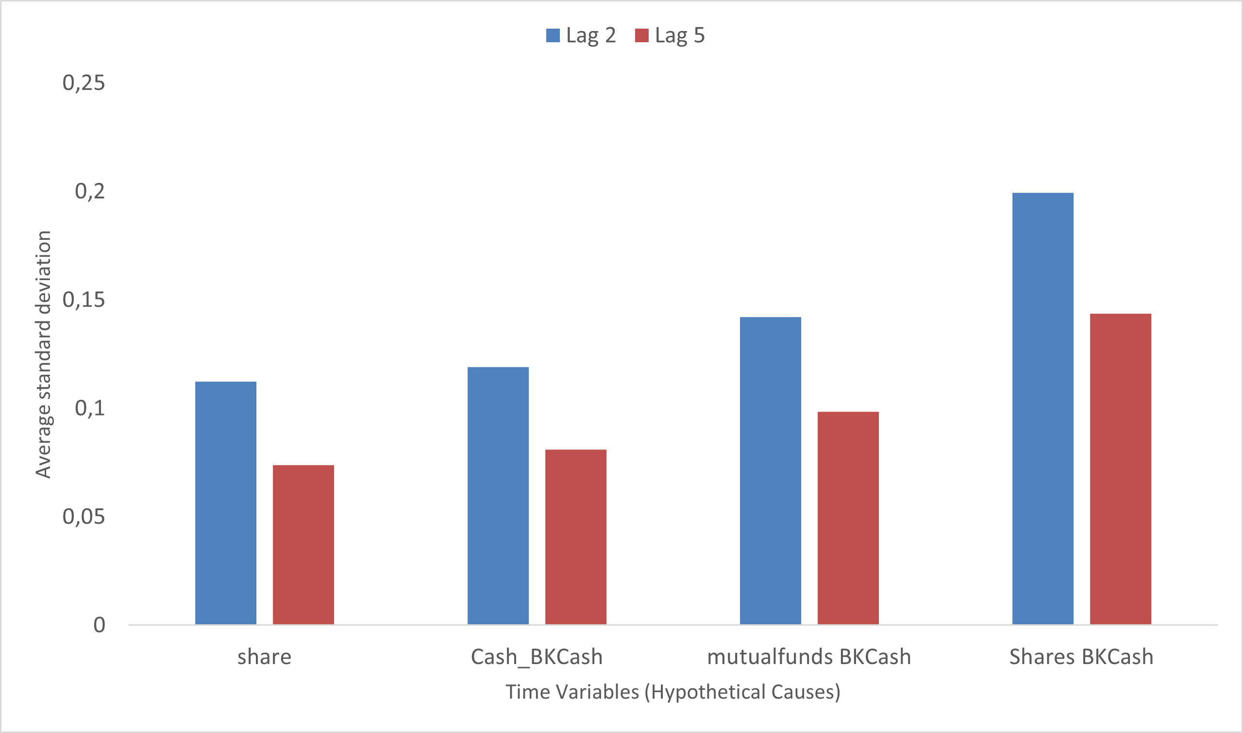
Figure 7: Average of the $\sigma_{\lambda}$ for lags 2 and 5 for different hypothetical causes (time series variables)

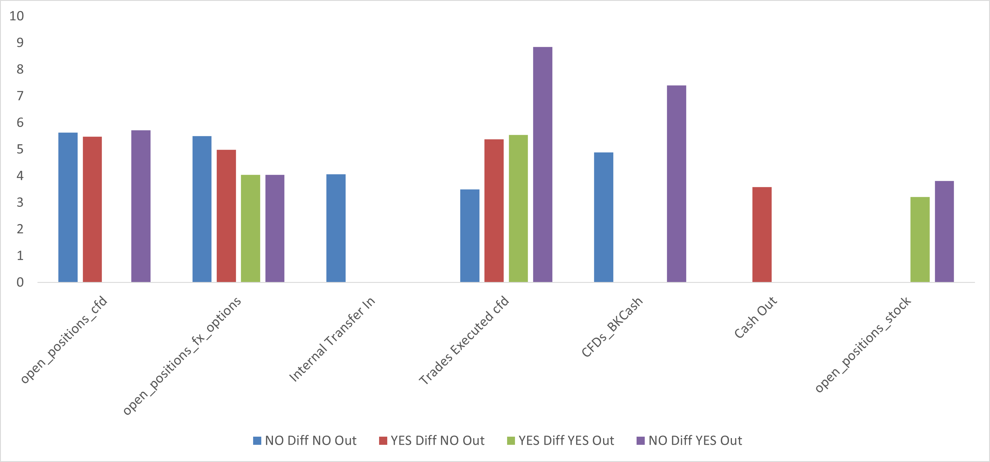
Figure 8: Granger Cause $\log(1/(p-value))$ values for different hypothetical causes (time series variables) and experiments with/without differentiation and outliers with lag=2

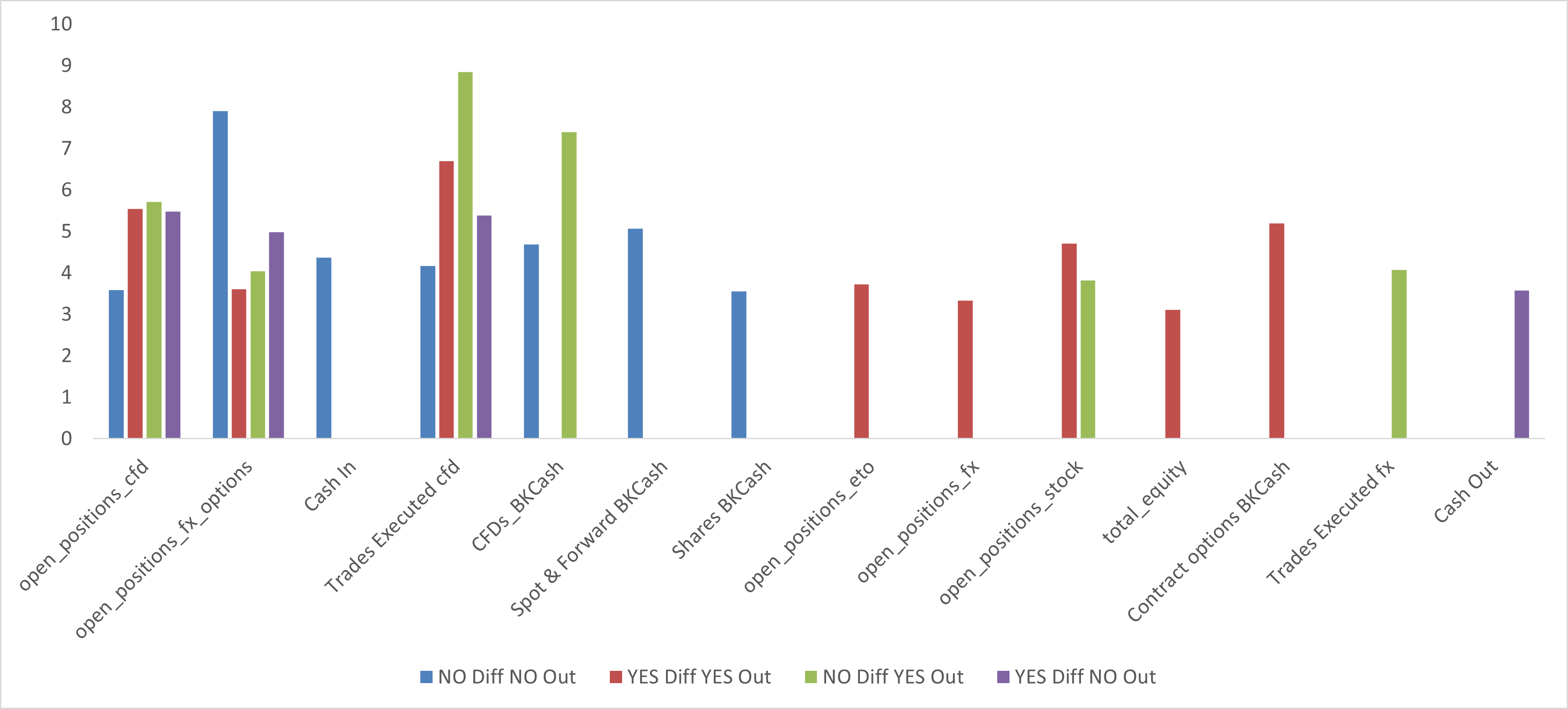
Figure 9: Granger Cause $\log(1/(p-value))$ values for different hypothetical causes (time series variables) and experiments with/without differentiation and outliers with lag=5

We can conclude that with greater lags, 5 or more, values only get smoother but patterns look the same (In Figure 10 we can see results for lag 10). This verifies the theoretical setup presented in this document in that, for greater lags the standard deviation of the explanatory power of their largest eigenvalue ($\sigma_{\lambda}$) is higher, and this implies a higher probability that the two variables deviate from independence based on the Tracy-Widom distribution towards a structured (causal) relationship.

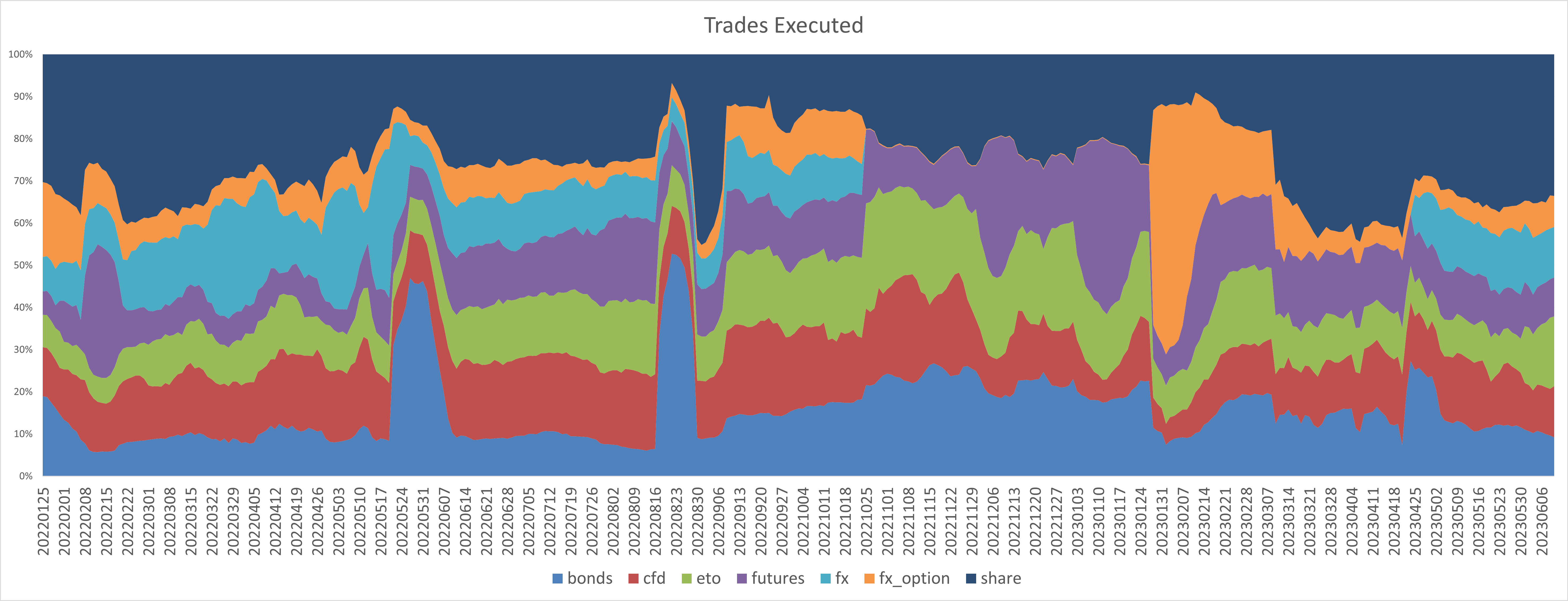
Figure 10: Broker trades executed vs cash balance, value of $\sigma_{\lambda}$ for lag 10

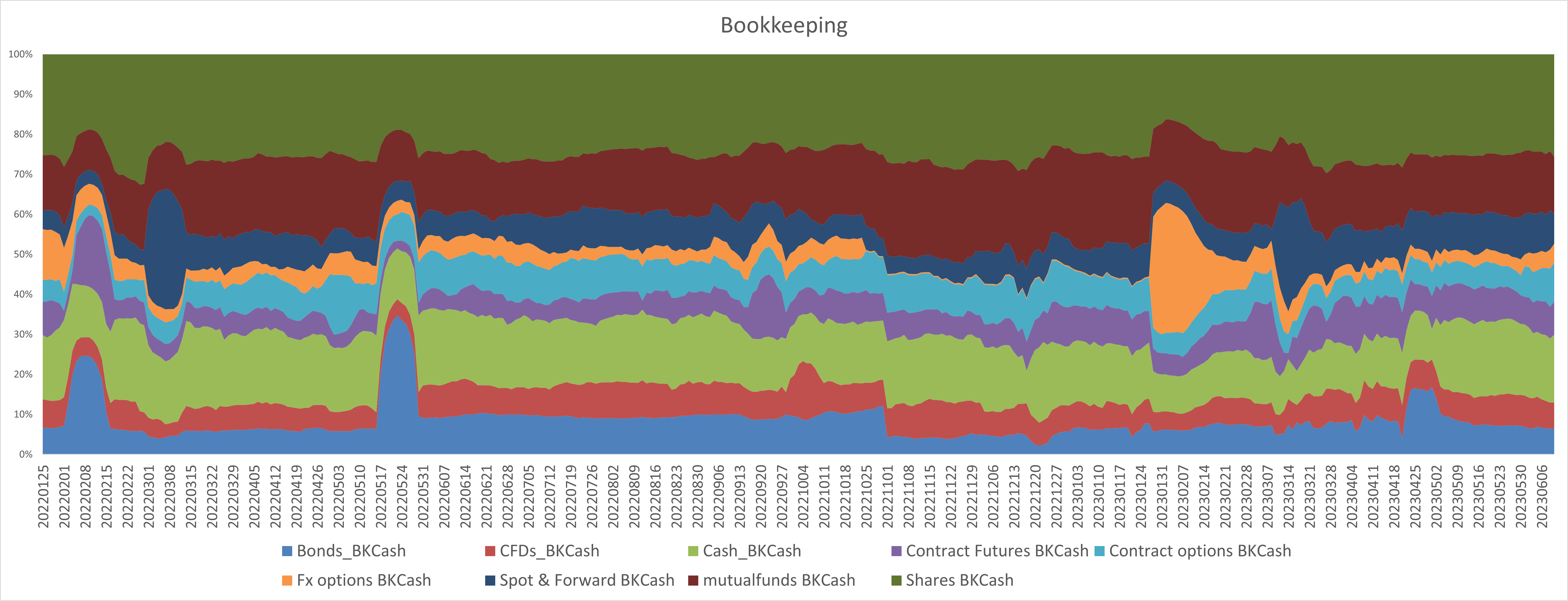
Figure 11: Bookkeeping cash, value of $\sigma_{\lambda}$ for lag 10, cash balance vs broker trading transactions

5 Conclusion

A systematic approach to measure and monitor structural relationships in time, which are related to causal relationships, is presented. The method is based on monitoring the time series of the standard deviation of the explanatory power of the first eigenvalue for multiple lags in lagged correlation matrices, which is related to the Tracy-Widom distribution from RMT. These matrices consist on $2\times 2$ correlation matrices between an hypothetical causal variable and the respective effect variable. The different time series for different causal variables given the same effect variable are compared. The method is simple and fast, allowing to avoid biases produced by other statistical tests such as Granger Causality test. The method is applied to analyse the structural or causal dependencies between daily monetary flows in a retail brokerage business. This allows practitioners to understand the causal dynamics between these flows being able to control for liquidity risk in banks or other financial institutions. The method can be applied to monitor causal or structural dependencies in time in any particular dataset. Extreme values of the indicator can serve for risk management or alpha signal purposes.

References

- [1] V A Marčenko and L A Pastur. Distribution of eigenvalues for some sets of random matrices. Mathematics of the USSR-Sbornik, 1(4):457, apr 1967.
- [2] David S. Dean and Satya N. Majumdar. Extreme value statistics of eigenvalues of gaussian random matrices. Phys. Rev. E, 77:041108, Apr 2008.
- [3] Eugene P. Wigner. Characteristic vectors of bordered matrices with infinite dimensions. Annals of Mathematics, 62(3):548–564, 1955.
- [4] Eugene P. Wigner. On the distribution of the roots of certain symmetric matrices. Annals of Mathematics, 67(2):325–327, 1958.
- [5] Waltraut J. Stein. How values adhere to facts: An outline of a theory*. The Southern Journal of Philosophy, 7(1):65–74, 1969.
- [6] Stuart Geman. A Limit Theorem for the Norm of Random Matrices. The Annals of Probability, 8(2):252 – 261, 1980.
- [7] Z. D. Bai. Methodologies in spectral analysis of large dimensional random matrices, a review. Statistica Sinica, 9(3):611–662, 1999.
- [8] Robb J. Muirhead. Aspects of multivariate statistical theory. In Wiley Series in Probability and Statistics, 1982.
- [9] A. G. Constantine. Some Non-Central Distribution Problems in Multivariate Analysis. The Annals of Mathematical Statistics, 34(4):1270 – 1285, 1963.
- [10] T. W. Anderson. Asymptotic Theory for Principal Component Analysis. The Annals of Mathematical Statistics, 34(1):122 – 148, 1963.
- [11] Robb J. Muirhead. Latent roots and matrix variates: A review of some asymptotic results. The Annals of Statistics, 6(1):5–33, 1978.
- [12] Wikipedia. Tracy–Widom distribution — Wikipedia, the free encyclopedia. http://en.wikipedia.org/w/index.php?title=Tracy%E2%80%93Widom%20distribution&oldid=1158407177, 2023. [Online; accessed 10-July-2023].
- [13] C. W. J. Granger. Investigating causal relations by econometric models and cross-spectral methods. Econometrica, 37(3):424–438, 1969.