Predicting Tuberculosis from Real-World Cough Audio Recordings and Metadata

Abstract

Tuberculosis (TB) is an infectious disease caused by the bacterium Mycobacterium tuberculosis and primarily affects the lungs, as well as other body parts. TB is spread through the air when an infected person coughs, sneezes, or talks. Medical doctors diagnose TB in patients via clinical examinations and specialized tests. However, coughing is a common symptom of respiratory diseases such as TB. Literature suggests that cough sounds coming from different respiratory diseases can be distinguished by both medical doctors and computer algorithms. Therefore, cough recordings associated with patients with and without TB seems to be a reasonable avenue of investigation. In this work, we utilize a very large dataset of TB and non-TB cough audio recordings obtained from the south-east of Africa, India, and the south-east of Asia using a fully automated phone-based application (Hyfe), without manual annotation. We fit statistical classifiers based on spectral and time domain features with and without clinical metadata. A stratified grouped cross-validation approach shows that an average Area Under Curve (AUC) of approximately $0.70\pm 0.05$ both for a cough-level and a participant-level classification can be achieved using cough sounds alone. The addition of demographic and clinical factors increases performance, resulting in an average AUC of approximately $0.81\pm 0.05$. Our results suggest mobile phone-based applications that integrate clinical symptoms and cough sound analysis could help community health workers and, most importantly, health service programs to improve TB case-finding efforts while reducing costs, which could substantially improve public health.

Keywords tuberculosis  $\cdot$ cough  $\cdot$ prediction  $\cdot$ audio  $\cdot$ machine learning  $\cdot$ deep learning

1 Introduction

Tuberculosis (TB) is one of the leading causes of death worldwide, with an estimated 1.5 million deaths in 2020 alone [1]. TB has a significant impact on economic development, has a disproportionate impact on vulnerable populations, and is increasingly due to drug resistant strains which are more difficult to treat. Thus, the eradication of TB is essential to save lives, reduce poverty, protect the most vulnerable, and safeguard against the spread of drug-resistant forms of the disease [2].

A major impediment to TB eradication is the difficulty in finding cases. Approximately $40\%$ of people with TB are not diagnosed or reported to public health authorities because of challenges in accessing health facilities or failure to be tested or treated when they do. The development of low-cost, non-invasive digital screening tools would help to address this challenge. Cough has traditionally been used to identify people who may have TB and to monitor treatment [3, 4, 5]. Advances in acoustic AI promises to passively detect and monitor cough and thus improve case finding [6, 7, 8, 9]. Furthermore, classification of coughs based on their sound may identify which individuals are most likely to have TB and thus help triage who should be prioritized for microbiological testing. Several previous studies have demonstrated the potential for cough sounds to be used to screen for TB [10, 11, 12, 13, 14, 15, 16, 17], though these were typically done in small samples and limited settings. Further development and evaluation of the diagnostic accuracy of AI algorithms for distinguishing tubercular from non-tubercular coughs are critical to move the field forward.

The CODA TB DREAM Challenge [18] is a major opportunity for advancing cough based diagnostics for TB. In brief, the Challenge collected data from people who presented to clinics across $7$ countries with new or worsening cough for at least $2$ weeks. Elicited coughs were recorded using the Hyfe Research app [19]. Individuals were then comprehensively evaluated for TB with molecular and culture testing of their sputa. The Challenge made this data publicly available so that AI experts could use it to develop and test algorithms to predict TB status using features extracted from elicited coughs, either in the presence or absence of demographic and clinical factors used routinely for TB screening. The Challenge released a training data set that could be used to develop diagnostic algorithms. Groups who complied with the constraints of the Challenge submitted these algorithms to SAGE who evaluated their performance using a hold-out data set. In contrast, because the authors were involved in the data collection and excluded from participating in the official challenge, in this work we exclusively used the publicly available training data to develop and test our diagnostic algorithms.

Specifically, we attempted to predict TB using the training dataset made available in the CODA TB DREAM challenge, including (a) cough audio recordings (Cough-only Experiment) and (b) demographic and clinical metadata along with cough audio recordings (Cough+Metadata Experiment). Clinical data includes a list of variables that are allowed to be used in the prediction model, such as age, sex, heart rate, temperature, and others. Well-known machine learning algorithms were used for both tasks. Cough audio recordings were modeled using low-level descriptors (LLDs), i.e. features extracted from audio signals and represent basic properties of the sound, such as its pitch, loudness, and timbre. Some common examples of LLDs in audio analysis include spectral features that describe the energy distribution of a specific part of the audio waveform, such as spectral centroid, flatness, spread, and others. On the other hand, spectrotemporal features describe the distribution of energy over time across different frequency bands. Examples of features in this category include Mel-frequency cepstral coefficients (MFCCs), linear prediction coefficients (LPCs), log-mel spectrograms, and chroma features[20]. Furthermore, temporal LLDs that describe time-domain characteristics of the audio signal, such as zero-crossing rate, energy, and amplitude envelope, are also used. Such feature sets have been successfully used in automatic cough detection [21, 22].

In Cough-only Experiment, we additionally used deep learning algorithms (two-dimensional convolutional neural networks - 2D-CNNs) [23] operating on spectrotemporal features obtained from the cough audio signals. Different convolutional architectures are trained on the spectrotemporal representations in a similar manner to neural networks trained on images for tasks such as object detection [24] and image segmentation [25]. In audio processing, a spectrotemporal representation is suitable as an image-like input, as proved in many works [26, 27, 28, 29]. Such approaches have also been successfully applied in cough recognition [30, 31]. In Cough+Metadata Experiment, the presence of metadata in tabular form led us to an approach that trains models jointly with metadata and cough audio features. For this, we used conventional ML models (not CNNs) that are able to handle tabular data well. Areas under Receiver Operating Curve (ROC-AUCs) are provided as performance metrics, for two reasons: (a) ROCs are a convenient way to assess the trade off between sensitivity and specificity when projecting the use of a diagnostic tool in screening versus confirmation use cases, and (b) AUC evaluates the ability of a classifier to prioritize positive instances over negative instances in terms of ranking, compared to other measures such as accuracy, which assesses the correct identification of true and false positives based on a specific decision threshold. AUC is considered a more inclusive measure of performance, regardless of the threshold chosen.

The rest of the paper is organized as follows: Section 2 presents the details of the dataset. Section 3 discusses our approach for Cough-only Experiment while Section 4 does the same for Cough+Metadata Experiment. Finally, Section 5 discusses the results and Section 6 concludes this work.

2 Dataset

The data are from health centers in $7$ countries (India, Philippines, South Africa, Uganda, Vietnam, Tanzania, Madagascar). The clinical research included the evaluation of all individuals who were 18 years of age or older and visited outpatient health centers for any health concern. Those who had a new or worsening cough that persisted for a minimum of two weeks were selected to participate in the study.

During the initial visit, a survey was conducted to gather standard demographic and clinical information from the participants. Additionally, samples of sputum were collected for tuberculosis TB testing. As part of the study, the participants were requested to cough, and the cough sounds were recorded using the Hyfe Research app. The app guides the participants with a countdown (3-2-1) and prompts them to cough, capturing approximately half a second of the "explosive" sounds within a five-second timeframe. This process is repeated five times. Cough sounds identified as coughs by the Hyfe cough prediction algorithm are included for analysis. It is important to note that the number of solicited coughs may vary for each participant depending on how many times they coughed during each five-second recording interval. Moreover, the act of producing a solicited cough may trigger additional coughing, so the cough files in this dataset comprise a combination of solicited and spontaneous coughs. The sampling frequency of all recordings is $44100$ Hz but the signals are sub-sampled for each experiment (more information in the following sections). In total, $9772$ sounds were analyzed. A statistical review of the dataset is illustrated in Table 1.

Table 1: Statistical review of the dataset.

Metric	TB+	TB-	Total
Participants	297	810	1107
Total coughs	2930	6842	9772
Average number of coughs/participant ($\pm$ std)	10.06 ($\pm$ 6.48)	8.65 ($\pm$ 5.15)	9.03 ($\pm$ 5.7)
Minimum number of coughs/participant	3	3	-
Maximum number of coughs/patient	50	37	-
Total duration of coughs (minutes)	24.41	57.01	81.43

Moreover, in Table 2 we present a list of demographic and clinical metadata used as features in Cough+Metadata experiment.

Table 2: Demographic and clinical data used as features in Cough+Metadata experiment.

Clinical or demographic datum	Description	Unit of measurement
Age	Age calculated as date of collection - date of birth if known. If date of birth is unknown, reported age at time of collection.	Years
Sex	Sex at birth reported by participant	Binary (male or female)
Height	The height of the participant	Centimeters
Weight	The weight of the participant	Kilograms
Reported duration of coughing	Self reported duration of current cough (days)	Days
Prior TB	Self reported status of whether the participant had or been told to have TB	Binary (yes or no)
Prior TB (Pulmonary)	Self reported status of whether the participant had or been told to have pulmonary TB	Binary (yes or no)
Prior TB (Extrapulmonary)	Self reported status of whether the participant had or been told to have extrapulmonary TB	Binary (yes or no)
Prior TB (Unknown)	Self reported status of whether the participant had or been told to have neither pulmonary nor extrapulmonary TB	Binary (yes or no)
Hemoptysis	Self reported status of whether the participant has ever coughed blood	Binary (yes or no)
Heart Rate	The heart rate of the participant measured at baseline	Beats per minute
Temperature	The temperature of the participant measured at baseline	Celsius
Smoke last week	Self reported status of whether the participant used combustible tobacco and/or vaping products in the last 7 days.	Binary (yes or no)
Fever	Self reported status of whether the participant had felt or experienced fever in the last 30 days.	Binary (yes or no)
Night sweats	Self reported status of whether the participant had experienced fever in the last 30 days.	Binary (yes or no)
Weight loss	Self reported status of whether the participant had experienced weight loss in the past 30 days.	Binary (yes or no)

3 Features

In this work we have utilized a series of audio features. The literature review suggests many different feature sets for compactly modeling sounds signals but most of these features were invented for audio, music, and speech signal use cases. Cough is a non-stationary signal, that is, it quickly changes over time. Thus we need to process it in short segments (the so-called frames) that are approximately stationary. Stationarity implies that temporal and spectral characteristics inside a frame do not significantly change. The length of each frame should be long enough to reliably estimate a feature set but short enough to ensure the measured features are representative of the whole frame. For these reasons, the usual frame length is around $20-50$ ms. For example, a $50$-ms window slides on the cough waveform with a step of $25$ ms (the so-called step or hop size or frame rate). This way, we have a $50\%$ overlap between successive frames. Finally, each frame is windowed (multiplied by a function in time that has desirable properties in the spectral domain) by a Hamming window. This process is illustrated in Fig. 1. However, this approach leads to a large number of features per audio signal. Statistical summarization is a convenient way to reduce their number.

3.1 Low Level Descriptors

To avoid the dimensionality curse [32, 33], we would like to focus on features that are relatively low in number but sufficiently representative of the cough audio signal. There seems to be an agreement that temporal and spectral features (jointly termed as acoustic features) combined are useful up to a certain level [34]. For our task we choose a set of LLDs consisting of temporal features like energy, Zero Crossing Rate, and Intensity, enriched by a more complex set of LLDs that includes Spectral measures (flux, entropy, 90% rolloff, centroid, spread), and spectrotemporal measures such as Mel-Frequency Cepstral Coefficients (MFCCs) and log-filterbank spectrograms.

We will now briefly discuss the selected acoustic features and their properties that make them suitable for our task. In what follows, we consider an audio frame $x[n]$ and a chosen windowing function $w[n]$ with support in $[n-N,n+N]$.

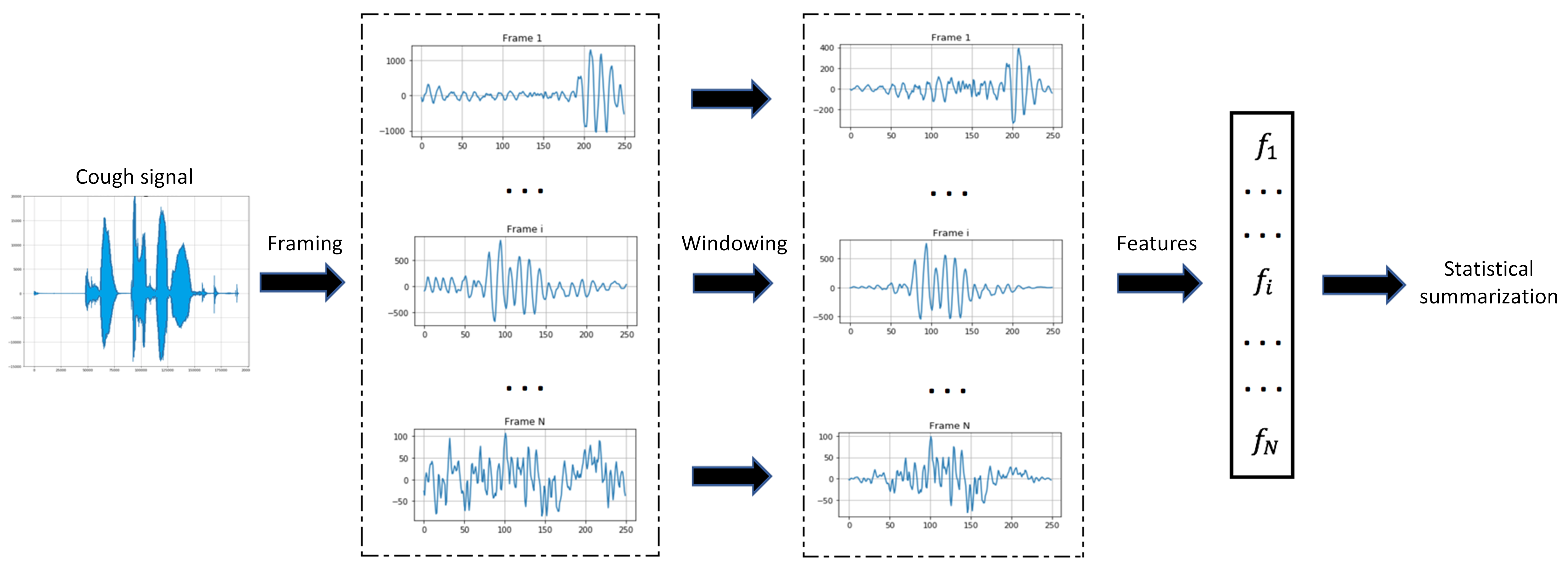
Figure 1: Feature Extraction Pipeline.

3.1.1 Temporal Features

1. Energy: the energy of a frame is a measure of the audio signals "size" or "strength", and is defined as

   $$E=\frac{1}{2N+1}\sum_{n=-\infty}^{+\infty}x[n]^{2}w^{2}[n]$$ (1)

2. Zero-crossing Rate: the ZCR provides some rough information about the frequency distribution of the speech signal and is defined as the number of times a signal crosses the horizontal (time) axis: a high frequency signal should have a high number of zero crossings while a low frequency signal should have a low number of zero crossings. ZCR denotes the rate of sign-changes of the signal during the duration of a particular frame. The mathematical definition of ZCR is

   $$ZCR=\frac{1}{2N+1}\sum_{n=-\infty}^{+\infty}\frac{1}{2}\left|\mathrm{sgn}(x[n])-\mathrm{sgn}(x[n-1])\right|x[n]w[n]$$ (2)

   where $\mathrm{sgn}[\cdot]$ is the signum function.

3. Intensity: the acoustic intensity of a sound is a physical quantity that can be defined as the average flow of energy (power) through a unit area measured in Watts per square meter. The human auditory system can detect a wide range of intensities, starting from $10^{-12}$ Watts per square meter and reaching up to $10$ Watts per square meter. These two extremes correspond to the threshold of hearing and the threshold of pain, respectively. Expressed in dB, the intensity of a signal $x[n]$ in air is defined as

   $$I=10\log_{10}\frac{1}{P_{0}}\left[\frac{1}{N}\sum_{n=-\infty}^{+\infty}(x[n]w[n])^{2}\right]$$ (3)

   where $P_{0}$ equals $2\times 10^{-5}$ Pa.

3.1.2 Spectral Features

1. Spectral Centroid: the spectral centroid (SC) is simply the center of gravity of the spectrum of a frame. It is computed considering the spectrum as a distribution which values are the frequencies and the probabilities to observe these frequencies are the normalized amplitude values. Let $X[k]$ be the N-point Fast Fourier Transform of the audio frame. Then the SC is defined as

   $$SC=\frac{\sum_{k=0}^{N-1}{kX[k]}}{\sum_{k=0}^{N-1}X[k]}$$ (4)

2. Spectral Spread: the spectral spread (SS) denotes the second central moment of the spectrum of the speech frame. The spectral spread describes the average deviation of the spectrum around its centroid, which is commonly associated with the bandwidth of the signal. Noise-like signals have usually a large spectral spread, while individual tonal sounds with isolated peaks will result in a low spectral spread. It is defined as

   $$SS=\sqrt{\frac{\sum_{k=0}^{N-1}(k-C)^{2}X[k]}{\sum_{k=0}^{N-1}X[k]}}$$ (5)

3. Spectral Roll-off: the 90%-spectral roll-off is the frequency so that 90% of the signal energy is contained below this frequency.

4. Spectral Entropy: the Spectral entropy (SE) of a signal is a measure of its spectral power distribution. The concept is based on the Shannon entropy, or information entropy, in information theory. The SE treats the signal’s normalized power distribution in the frequency domain as a probability distribution, and calculates the Shannon entropy of it. The Shannon entropy in this context is the spectral entropy of the signal. We can define the spectral entropy in terms of power spectrum and probability distribution of a signal. If $S[k]=|X[k]|^{2}$ is the power spectrum of an audio frame, then $P[k]$ is its probability distribution given by

   $$P[k]=\frac{S[k]}{\sum_{i=0}^{N-1}S[i]}$$ (6)

   Finally, the SE is given by

   $$SE=-\frac{\sum_{m=1}^{N}P[m]\log_{2}P[m]}{\log_{2}N}$$ (7)

5. Spectral Flux: the spectral flux (SF) is a measure of how quickly the power spectrum of a signal is changing, calculated by comparing the power spectrum for one frame against the power spectrum from the previous frame. More precisely, it is usually calculated as the 2-norm (also known as the Euclidean distance) between the two normalized spectra. If $X_{t}[k]$ is the normalized power spectrum of frame $t$, then SF can be calculated as

   $$SF[k]=\left(\sum_{k=b_{1}}^{k=b_{2}}|X_{t}[k]-X_{t-1}[k]|^{P}\right)^{1/P}$$ (8)

   where $b_{1}$ and $b_{2}$ are the band edges, in frequency bins, over which we calculate the SF. Usually, $b_{1}=0$ and $b_{2}=N$, and $P=2$.

3.1.3 Spectrotemporal features

1. Log-mel spectrogram: The log-mel spectrogram is a specific type of spectrogram that combines two transformations: the Mel scale and the logarithmic compression. To create a log-mel spectrogram, the audio signal is first divided into short overlapping frames. Then, the Fourier transform is applied to each frame, resulting in a spectrogram. Next, the spectrogram is transformed to the mel scale using a filterbank that converts linear frequency values to mel scale values. This mel scale is defined as

   $$Mel(f)=2595\log\left(1+\frac{f}{700}\right)$$ (9)

   and is a perceptual scale of pitches judged by listeners to be equal in distance from one another. The log-mel spectrogram provides a concise representation of the audio signal that captures both frequency and temporal information.

2. Mel-frequency Cepstral Coefficients: Similarly to the log-mel spectrogram, Mel Frequency Cepstral Coefficients (MFCCs) model the spectral energy distribution in a perceptually meaningful way, that is, MFCCs is a cepstral representation where the frequency bands are not linear but distributed according to the mel scale. Following computation of log-mel spectrogram, the Discrete Cosine Transform (DCT) is applied on the list of mel-log powers, as if it were a signal. The MFCCs are the amplitudes of the resulting signal.

Parameters for generating all features are shown in Table 3 and an example of TB vs non-TB cough recordings, downsampled to $22050$ Hz, along with their corresponding spectrotemporal representations is depicted in Figure 2.

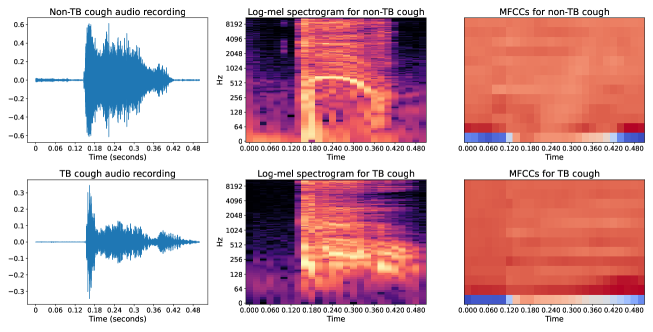
Figure 2: Audio recordings, log-mel spectrograms, and mel-frequency cepstral coefficients for two cough sounds, one from a TB patient (upper three panels), and one from a healthy patient (lower three panels).

For standard ML models that require vectorized inputs, a set of statistics will be applied on these LLDs in order to summarize features from all frames of the audio signal. Let $v=\{x_{1},x_{2},x_{3},\cdots,x_{N}\}$ denote a sample LLD consisting of $N$ values. We define:

1. mean: the average value of an LLD

   $$\hat{x}=\frac{1}{N}\sum_{n=1}^{N}x_{n}$$ (10)

2. standard deviation: measures the amount of variation or dispersion of an LLD

   $$s=\sqrt{\frac{1}{N-1}\sum_{n=1}^{N}(x_{n}-\hat{x})}$$ (11)

3. skewness: measures the asymmetry of the sample distribution of an LLD about its mean

   $$b_{1}=\frac{\frac{1}{N}\sum_{n=1}^{N}(x_{n}-\hat{x})^{3}}{\left[\frac{1}{N-1}\sum_{n=1}^{N}(x_{n}-\hat{x})^{2}\right]^{3/2}}$$ (12)

4. kurtosis: measures the "tailedness" of the sample distribution of an LLD

   $$g_{2}=\frac{(N+1)N}{(N-1)(N-2)(N-3)}\cdot\frac{\sum_{n=1}^{N}(x_{n}-\hat{x})^{4}}{\left[\sum_{n=1}^{N}(x_{n}-\hat{x})^{2}\right]^{2}}-3\frac{(N-1)^{2}}{(N-2)(N-3)}$$ (13)

and these will be the final features for each audio signal. Reasons for such a selection are ease of implementation, either directly or by open-source software, robustness, and relevance to the task.

Table 3: Feature extraction parameters.

Parameters for temporal and spectral features
Frame Size	Hop Size	FFT size
$0.05$ s	$0.025$ s	$1024$
Number of Features	Window Type	Sampling Frequency
$62$ per frame	Hanning	$16000$
Parameters for spectrotemporal features
Frame Size	Hop Size	FFT size
$0.04$ s	$0.02$ s	$2048$
Number of Filters or Coefficients	Window Type	Sampling Frequency
$128$ or $13$	Hanning	$22050$

4 Experiments

Implementations are carried out in Python [35], (v. 3.9), using LibROSA [36] (v. 0.9.2), Tensorflow [37] (v. 2.10), and Sci-kit Learn APIs [38] (v. 1.22), while mathematical details can be found in [39, 23]. A list of machine learning models and their hyperparameters (tuned or fixed) are shown in Table 4. All classifiers are used for both experiments except for CNNs, which are only utilized in the Cough-Only experiment.

Table 4: Machine learning models with their hyperparameters.

Algorithm	Hyperparameters (constant and tuned)
Logistic Regression (LR)	Solver: LBFGS Penalty: L2 C: tuned from $10^{-5}$ to $1.0$
Support Vector Machine (SVM)	C: tuned from $0.01$ to $5$ $\gamma$: tuned from $10^{-1}$ to $10^{-5}$
Multi-Layer Perceptron (MLP)	$\alpha$: tuned from $10^{-5}$ to $1.0$ Hidden layer size: $5$ Neuron number: tuned from $256$ up to $4$ per layer, in decreasing order Solver: Adam Learning rate: $0.001$ Activation: ReLU
Random Forest (RF)	Estimators: tuned from $100$ to $500$ Maximum number of features: tuned between square root and log2 Maximum depth: tuned between $4,6$, and $8$ Split criterion: tuned between Gini and Entropy
AdaBoost (AB)	Number of estimators: tuned from $10$ to $500$ Learning rate: tuned from $10^{-4}$ to $1.0$
CNN (Cough-Only experiment)	Convolution layers depth: tuned from $2,3$ and $4$ Filter size: [$16,32$], [$16,32,64$], [$16,32,64,128$] (first to last layer) Kernel size = $3\times 3$ Batch Normalization: tuned between yes and no (in between convolution and activation layers) Pooling: tuned between Max and Average Dropout: tuned between $0.25$ and $0.5$ (between dense layers) Activation: ReLU Number of dense Layers: $3$ Neuron number in dense layers: [$1024,256,128$] (first to last layer)

4.1 Cough-only Experiment

In the first experiment, TB prediction should be based on audio cough sounds only. Given the amount of available recordings ($9772$ files), deep learning approaches (CNNs) are also suitable for the classification task, along with conventional machine learning algorithms. The latter use high-dimensional vectors of temporal and spectral features as mentioned in Section 3, while CNNs use spectrotemporal representations of cough sounds as input features. A $10$-fold stratified grouped cross-validation (CV) was selected to examine model performance. The proposed CV scheme ensures that coughs from each participant were either in the train set or the test set (and not in both). Different CNN-based architectures are tested but the one shown in Fig. 3 is the one with the best average AUC results. Cough predictions are also averaged per participant.

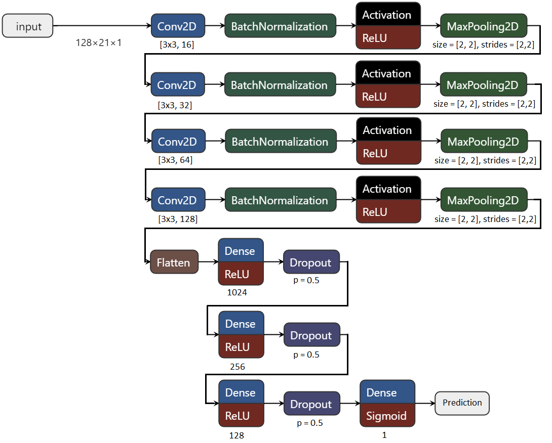
Figure 3: Best CNN architecture. $[MxN,L]$ under each Conv 2D block denote the filter size and the number of filters, respectively. $p=0.5$ under each Dropout block denotes the dropout probability while "size" and "strides" are parameters of the MaxPooling layer. Finally, numbers under Dense layers provide the number of neurons for each layer.

Regarding training, a batch size of $32$ was chosen along with a number of $40$ epochs for training, a number small enough to prevent overfitting. Approaches with a validation set resulted in slightly worse performance, probably due to reducing the training set size. When training a model, it is often useful to lower the learning rate as the training progresses. We choose the Cosine Decay with restarts [40] scheduler that applies a cosine decay function with restarts to an optimizer step, given a provided initial learning rate (set to $0.0001$). It requires a step value (set to $4000$) to compute the decayed learning rate. The selected optimizer was Adam [41] with a binary cross-entropy loss function.

In Figure 4 we present a boxplot of AUCs averaged over a $10$-fold cross-validation, assessing both isolated cough sounds and aggregated per participant.

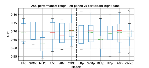
Figure 4: Cough-only experiment: boxplots of AUC values for all models. Left: per-cough assessment. Right: per-participant assessment. Red solid and green dashed lines denote mean and median value, respectively. For model abbreviations, see Table 4.

It should be noted that while the CNN outperforms other methods on average in isolated cough classification (AUC $0.70\pm 0.05$), when coughs are aggregated, a simple Logistic Regression achieves a higher average AUC ($0.69\pm 0.07$).

4.2 Cough+Metadata Experiment

In this experiment, we decided to jointly train a model on both the demographic and clinical metadata and the cough audio features. Since training 2-dimensional spectrotemporal data jointly with tabular data (metadata) is feasible but not straightforward, log-mel spectrograms and MFCCs were flattened to a 1-dimensional vector and concatenated to the rest of features in a tabular form.

In this section, we briefly present the classification pipeline we follow in this experiment. Features are extracted, stacked, statistically summarized, and fed to the classifiers as inputs. Feature scaling is performed whenever necessary. We use stratified $5$-fold cross-validation to tune hyperparameters. Final predictions are made on several hold-out test sets, defined by a stratified, grouped $10$-fold cross-validation split. Hyperparameters were tuned in a nested stratified grouped $5$-fold cross-validation.

In Figure 5 we present a boxplot of AUCs for our $10$-fold CV, assessing both isolated cough sounds and aggregated per participant.

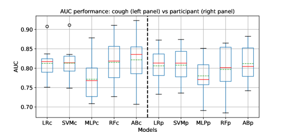
Figure 5: Cough+Metadata experiment: boxplots of AUC values for all models. Left: per-cough assessment. Right: per-participant assessment. Red solid and green dashed lines denote median and mean value, respectively. For model abbreviations, see Table 4.

An ensemble model, AdaBoost, achieves an average AUC of $0.82\pm 0.05$ and an average AUC of $0.81\pm 0.04$ is obtained per cough sound and per participant, respectively.

5 Discussion

Figures 4 and 5 show that clinical and demographic data increase average AUC performance in both cough-based and participant-based classification. More specifically, in Cough-only experiment, none of the conventional ML methods showed a mean or median AUC greater than $0.70$ on a cough-basis classification. On the contrary, the CNN model achieved a mean and median AUC just above $0.70$. On a participant-basis classification, all models performed better on average, suggesting that aggregating probabilities might be beneficial to the prediction system. In Cough+Metadata experiment, AUC distributions are less spread out and both the average and median AUC is well above $0.80$ for all models but MLPs. It is interesting to note that Adaptive Boosting (AB) performs best on average in single cough classification but similarly to simpler models (LR, SVM) when aggregating cough probabilities. This behavior is consistent in other models as well, indicating that weighted averaging of probabilities might worth exploring. Overall, one may conclude that Multi-Layer Perceptrons (MLPs) seem to perform worst in all cases and Logistic Regression (LR), a simple, fast, and well-known statistical model performs quite well compared to more advanced models such as Adaptive Boosting (AdaBoost) and ensemble learning methods such as Random Forests (RFs).

6 Conclusions and Future Work

In this work, we present Hyfe’s approach for diagnosing TB based solely on the publicly available training data from the CODA DREAM Challenge. We demonstrate the potential of both deep learning approaches and conventional features from audio processing as predictors for tuberculosis, along with standard demographic and clinical metadata. Results are encouraging, especially for models trained on both audio and tabular data. To our knowledge, this is the first study that compares machine learning techniques on such a diverse, large, automatically collected dataset of cough audio recordings. Importantly, our results on Cough+Metadata experiment are particularly relevant to TB control programs given the complexity and poor performance of conventional sputum microscopy [42]. If confirmed in larger community-based studies, our results suggest that the accuracy of cough sounds is sufficient for triaging which coughing patients should be prioritized for definitive TB diagnostic evaluation. This effort was not exhaustive and there are many improvements and alternatives which might further improve the audio analysis, starting from enriching the feature set and up to selecting different classifiers and feature selection schemes that have not been discussed in this work. In addition, there remain questions such as the optimal number of features, the most appropriate features that can model cough sounds adequately, the best classifier in terms of complexity, convergence speed, and accuracy, and the parameters of the analysis, among others. Moreover, the dataset used in his study provides a baseline dataset for researchers and engineers interested in developing statistical learning methods for TB prediction. These preliminary results suggest that mobile phone-based apps that integrate clinical symptoms and cough sound analysis could help community health workers to identify TB patients. If integrated into digital health systems [43, 44] of low-resource countries with a high burden of TB, such as Nikshay [45, 46, 47] in India, such devices would also allow TB control programs to better understand the epidemiology and clinical management of those suspected of having TB.

Acknowledgments

The datasets used for the analyses described were contributed by Dr. Adithya Cattamanchi at USCF and Dr. Simon Grandjean Lapierre at University of Montreal and were generated in collaboration with researchers at Stellenbosch University (PI Grant Theron), Walimu (PIs William Worodria and Alfred Andama); De La Salle Medical and Health Sciences Institute (PI Charles Yu), Vietnam National Tuberculosis Program (PI Nguyen Viet Nhung), Christian Medical College (PI DJ Christopher), Centre Infectiologie Charles Merieux Madagascar (PIs Mihaja Raberahona & Rivonirina Rakotoarivelo), and Ifakara Health Institute (PIs Issa Lyimo & Omar Lweno) with funding from the U.S. National Institutes of Health (U01 AI152087), The Patrick J. McGovern Foundation and Global Health Labs.

References

- [1] Global tuberculosis report. Technical report, World Health Organization, 2021.
- [2] Alberto Matteelli, Adrian Rendon, Simon Tiberi, Seif Al-Abri, Constantia Voniatis, Anna Cristina C. Carvalho, Rosella Centis, Lia D’Ambrosio, Dina Visca, Antonio Spanevello, and Giovanni Battista Migliori. Tuberculosis elimination: where are we now? European Respiratory Review, 27(148), 2018.
- [3] Robert G Loudon and Sharon K Spohn. Cough frequency and infectivity in patients with pulmonary tuberculosis. American Review of Respiratory Disease, 99(1):109–111, 1969.
- [4] Richard D Turner and Graham H Bothamley. Cough and the transmission of tuberculosis. The Journal of infectious diseases, 211(9):1367–1372, 2015.
- [5] G Fochsen, K Deshpande, V Diwan, A Mishra, VK Diwan, and A Thorson. Health care seeking among individuals with cough and tuberculosis: a population-based study from rural India. The International Journal of Tuberculosis and Lung Disease, 10(9):995–1000, 2006.
- [6] SS Birring, T Fleming, S Matos, AA Raj, DH Evans, and ID Pavord. The leicester cough monitor: preliminary validation of an automated cough detection system in chronic cough. European Respiratory Journal, 31(5):1013–1018, 2008.
- [7] Cuong Pham. MobiCough: real-time cough detection and monitoring using low-cost mobile devices. In Intelligent Information and Database Systems: 8th Asian Conference, pages 300–309. Springer, 2016.
- [8] Daniyal Liaqat, Salaar Liaqat, Jun Lin Chen, Tina Sedaghat, Moshe Gabel, Frank Rudzicz, and Eyal de Lara. Coughwatch: Real-world cough detection using smartwatches. In 2021 IEEE International Conference on Acoustics, Speech and Signal Processing (ICASSP), pages 8333–8337. IEEE, 2021.
- [9] Liang Zhu, Trung Dũng Hà, Yi-Huan Chen, Haiyu Huang, and Pai-Yen Chen. A passive smart face mask for wireless cough monitoring: A harmonic detection scheme with clutter rejection. IEEE Transactions on Biomedical Circuits and Systems, 16(1):129–137, 2022.
- [10] Rahul Pathri, Shekhar Jha, Samarth Tandon, and Suryakanth GangaShetty. Acoustic epidemiology of pulmonary tuberculosis (TB) & Covid19 leveraging AI/ML. medRxiv, 2022.
- [11] Madhurananda Pahar, Marisa Klopper, Byron Reeve, Rob Warren, Grant Theron, and Thomas Niesler. Automatic cough classification for tuberculosis screening in a real-world environment. Physiological Measurement, 42(10):105014, 2021.
- [12] G. H. R Botha, G. Theron, R. M. Warren, M. Klopper, K. Dheda, P. D. van Helden, and T. R. Niesler. Detection of tuberculosis by automatic cough sound analysis. Physiological Measurement, 39(4):045005, 2018.
- [13] Brian H Tracey, Germán Comina, Sandra Larson, Marjory Bravard, José W López, and Robert H Gilman. Cough detection algorithm for monitoring patient recovery from pulmonary tuberculosis. In 2011 International Conference of the IEEE Engineering in Medicine and Biology Society, pages 6017–6020. IEEE, 2011.
- [14] Madhurananda Pahar, Marisa Klopper, Byron Reeve, Rob Warren, Grant Theron, Andreas Diacon, and Thomas Niesler. Automatic tuberculosis and covid-19 cough classification using deep learning. In 2022 International Conference on Electrical, Computer and Energy Technologies (ICECET), pages 1–9, 2022.
- [15] Madhurananda Pahar, Grant Theron, and Thomas Niesler. Automatic tuberculosis detection in cough patterns using NLP-style cough embeddings. In 2022 International Conference on Engineering and Emerging Technologies (ICEET), pages 1–6, 2022.
- [16] Geoffrey S Frost, Grant Theron, and Thomas R. Niesler. TB or not TB? Acoustic cough analysis for tuberculosis classification. In International Conference of Speech Communication Association, 2022.
- [17] Madhurananda Pahar, Igor Miranda, Andreas Diacon, and Thomas Niesler. Automatic non-invasive cough detection based on accelerometer and audio signals. Journal of Signal Processing Systems, 94(8):821–835, 2022.
- [18] SAGE Bionetworks. CODA TB DREAM challenge. https://www.synapse.org/#!Synapse:syn31472953/wiki/619711, 2023.
- [19] Hyfe Inc. Hyfe AI - detect and quantify cough. https://www.hyfe.ai/, 2023.
- [20] Meinard Müller. Fundamentals of Music Processing. Springer International Publishing, 2015.
- [21] Renard Xaviero Adhi Pramono, Syed Anas Imtiaz, and Esther Rodriguez-Villegas. Automatic cough detection in acoustic signal using spectral features. In 2019 International Conference of the IEEE Engineering in Medicine and Biology Society (EMBC), pages 7153–7156, 2019.
- [22] Prad Kadambi, Abinash Mohanty, Hao Ren, Jaclyn Smith, Kevin McGuinnes, Kimberly Holt, Armin Furtwaengler, Roberto Slepetys, Zheng Yang, Jae-sun Seo, Junseok Chae, Yu Cao, and Visar Berisha. Towards a wearable cough detector based on neural networks. In 2018 IEEE International Conference on Acoustics, Speech and Signal Processing (ICASSP), pages 2161–2165, 2018.
- [23] Ian J. Goodfellow, Yoshua Bengio, and Aaron Courville. Deep Learning. MIT Press, Cambridge, MA, USA, 2016.
- [24] Zhong-Qiu Zhao, Peng Zheng, Shou-tao Xu, and Xindong Wu. Object detection with deep learning: A review. IEEE Transactions on Neural Networks and Learning Systems, 30(11):3212–3232, 2019.
- [25] Liang-Chieh Chen, George Papandreou, Iasonas Kokkinos, Kevin Murphy, and Alan L Yuille. Deeplab: Semantic image segmentation with deep convolutional nets, atrous convolution, and fully connected CRFs. IEEE Transactions on Pattern Analysis and Machine Intelligence, 40(4):834–848, 2017.
- [26] Jianfeng Zhao, Xia Mao, and Lijiang Chen. Speech emotion recognition using deep 1d & 2d cnn lstm networks. Biomedical signal processing and control, 47:312–323, 2019.
- [27] Ossama Abdel-Hamid, Abdel-rahman Mohamed, Hui Jiang, Li Deng, Gerald Penn, and Dong Yu. Convolutional neural networks for speech recognition. IEEE/ACM Transactions on audio, speech, and language processing, 22(10):1533–1545, 2014.
- [28] Shawn Hershey, Sourish Chaudhuri, Daniel PW Ellis, Jort F Gemmeke, Aren Jansen, R Channing Moore, Manoj Plakal, Devin Platt, Rif A Saurous, Bryan Seybold, et al. Cnn architectures for large-scale audio classification. In 2017 IEEE International Conference on Acoustics, Speech and Signal Processing (ICASSP), pages 131–135. IEEE, 2017.
- [29] S Vishnupriya and K Meenakshi. Automatic music genre classification using convolution neural network. In 2018 international conference on computer communication and informatics (ICCCI), pages 1–4. IEEE, 2018.
- [30] Quan Zhou, Jianhua Shan, Wenlong Ding, Chengyin Wang, Shi Yuan, Fuchun Sun, Haiyuan Li, and Bin Fang. Cough recognition based on mel-spectrogram and convolutional neural network. Frontiers in Robotics and AI, 8, 2021.
- [31] Filipe Barata, Kevin Kipfer, Maurice Weber, Peter Tinschert, Elgar Fleisch, and Tobias Kowatsch. Towards device-agnostic mobile cough detection with convolutional neural networks. In 2019 IEEE International Conference on Healthcare Informatics (ICHI), pages 1–11, 2019.
- [32] Essam Debie and Kamran Shafi. Implications of the curse of dimensionality for supervised learning classifier systems: Theoretical and empirical analyses. Pattern Analysis & Applications, 22(2):519–536, 2019.
- [33] Eamonn Keogh and Abdullah Mueen. Curse of Dimensionality, pages 314–31. Springer US, Boston, MA, 2017.
- [34] Geoffroy Peeters. A large set of audio features for sound description (similarity and classification) in the cuidado project. CUIDADO Ist Project Report, 54(0):1–25, 2004.
- [35] Guido Van Rossum and Fred L Drake Jr. Python reference manual. Centrum voor Wiskunde en Informatica Amsterdam, 1995.
- [36] Brian McFee, Colin Raffel, Dawen Liang, Daniel PW Ellis, Matt McVicar, Eric Battenberg, and Oriol Nieto. librosa: Audio and music signal analysis in python. In Proceedings of the 14th python in science conference, volume 8, 2015.
- [37] Martín Abadi, Paul Barham, Jianmin Chen, Zhifeng Chen, Andy Davis, Jeffrey Dean, Matthieu Devin, Sanjay Ghemawat, Geoffrey Irving, Michael Isard, et al. TensorFlow: a system for Large-Scale machine learning. In 12th USENIX symposium on operating systems design and implementation (OSDI 16), pages 265–283, 2016.
- [38] F. Pedregosa, G. Varoquaux, A. Gramfort, V. Michel, B. Thirion, O. Grisel, M. Blondel, P. Prettenhofer, R. Weiss, V. Dubourg, J. Vanderplas, A. Passos, D. Cournapeau, M. Brucher, M. Perrot, and E. Duchesnay. Scikit-learn: Machine learning in Python. Journal of Machine Learning Research, 12:2825–2830, 2011.
- [39] Trevor Hastie, Robert Tibshirani, and Jerome Friedman. The Elements of Statistical Learning. Springer Series in Statistics. Springer New York Inc., New York, NY, USA, 2001.
- [40] Ilya Loshchilov and Frank Hutter. SGDR: Stochastic gradient descent with warm restarts. Learning, 10:3.
- [41] Diederik P. Kingma and Jimmy Ba. Adam: A method for stochastic optimization. Computing Research Repository, abs/1412.6980, 2014.
- [42] P.D.O. Davies and M. Pai. The diagnosis and misdiagnosis of tuberculosis. The International Journal of Tuberculosis and Lung Disease, 12(11):1226–1234, 2008.
- [43] Ntwali Placide Nsengiyumva, Benjamin Mappin-Kasirer, Olivia Oxlade, Mayara Bastos, Anete Trajman, Dennis Falzon, and Kevin Schwartzman. Evaluating the potential costs and impact of digital health technologies for tuberculosis treatment support. European Respiratory Journal, 52(5), 2018.
- [44] Marc Mitchell and Lena Kan. Digital technology and the future of health systems. Health Systems & Reform, 5(2):113–120, 2019.
- [45] Reema Arora, Ashwini Khanna, Nandini Sharma, Vishal Khanna, Kalpita Shringarpure, and Soundappan Kathirvel. Early implementation challenges in electronic referral and feedback mechanism for patients with tuberculosis using Nikshay–a mixed-methods study from a medical college TB referral unit of Delhi, India. Journal of Family Medicine and Primary Care, 10(4):1678, 2021.
- [46] Rajesh Kumar, Khalid Umer Khayyam, Neeta Singla, Tanu Anand, Sharath Burugina Nagaraja, Karuna D Sagili, and Rohit Sarin. Nikshay Poshan Yojana (NPY) for tuberculosis patients: Early implementation challenges in Delhi, India. Indian Journal of Tuberculosis, 67(2):231–237, 2020.
- [47] Surup Dey, Arathi P Rao, Ashwini Kumar, and Prakash Narayanan. Awareness & utilization of NIKSHAY and perceived barriers for tuberculosis case notification among the private practitioners in Udupi district, Karnataka. Indian Journal of Tuberculosis, 67(1):15–19, 2020.