Nature of the Schmid transition in a resistively shunted Josephson junction

Abstract

We study the phase diagram of a resistively shunted Josephson junction (RSJJ) in the framework of the boundary sine-Gordon model. Using the non-perturbative functional renormalization group (FRG) we find that the transition is not controlled by a single fixed point but by a line of fixed points, and compute the continuously varying critical exponent $\nu$. We argue that the conductance also varies continuously along the transition line. In contrast to the traditional phase diagram of the RSJJ —an insulating ground state when the shunt resistance $R$ is larger than $R_{q}=h/(2e)^{2}$ and a superconducting one when $R<R_{q}$— the FRG predicts the transition line in the plane $(\alpha,E_{J}/E_{C})$ to bend in the region $\alpha=R_{q}/R<1$ but we cannot discard the possibility of a vertical line at $\alpha=1$ ($E_{J}$ and $E_{C}$ denote the Josephson and charging energies of the junction, respectively). Our results regarding the phase diagram and the nature of the transition are compared with Monte Carlo simulations and numerical renormalization group results.

I Introduction.

Although the resistively shunted Josephson junction (RSJJ) [1] is one of the best-studied examples of dissipative quantum systems [2], its basic properties are still a matter of debate. Since the seminal work of Schmid and Bulgadaev (SB) on the quantum Brownian particle in a periodic potential (a problem that can be mapped on the RSJJ) [3, 4], the conventional view is that the junction is insulating when the shunt resistance $R$ is larger than the quantum of resistance $R_{q}=h/q^{2}$ ($q=2e$ is the Cooper pair charge) and superconducting when $R<R_{q}$ [5, 6, 7, 1] but for a long time there has been little experimental evidence [8, 9, 10, 11]. In a recent experiment no sign of the expected insulating phase was observed and the very existence of the dissipative quantum phase transition at $R=R_{q}$ has been questioned [12, 13, *Murani21], whereas the observation of the Schmid transition has been reported in another experiment [15]. On the other hand, using both the numerical renormalization group (NRG) and the functional renormalization group (FRG), it has been shown that when $\alpha=R_{q}/R<1$ an insulating-superconducting transition can be induced by varying the ratio $E_{J}/E_{C}$ between the Josephson coupling energy and the charging energy [16, 17], but these conclusions have been questioned [18, *Masuki22a].

In this paper, we reconsider the superconductor-insulator transition in a RSJJ, as shown in Fig. 1, where the Josephson junction is shunted by both a resistance and a capacitance [20]. The RSJJ can be described in the framework of the boundary sine-Gordon model originally studied by SB and defined by the Euclidean (imaginary-time) action [21]

$$S[\varphi]={} \frac{1}{2}\sum_{\omega_{n}}\left(\frac{\alpha}{2\pi}|\omega_{n}|+\frac{\omega_{n}^{2}}{2E_{C}}\right)|\varphi(i\omega_{n})|^{2}$$

$$-E_{J}\int_{0}^{\beta}d\tau\cos\varphi(\tau),$$ (1)

where $E_{J}$ is the Josephson coupling energy, $E_{C}=q^{2}/2C_{J}$ the charging energy and $C_{J}$ the capacitance of the junction. The field $\varphi$, which stands for the superconducting order parameter phase difference across the junction, is a noncompact variable which satisfies periodic boundary conditions in imaginary time, $\varphi(0)=\varphi(\beta)$, and $\omega_{n}=2n\pi T$ ($n$ integer) is a bosonic Matsubara frequency. $\beta=1/T$ is the inverse temperature and we consider only the zero-temperature limit $\beta\to\infty$ (we set $\hbar=k_{B}=1$ throughout the paper). We assume a ultraviolet (UV) frequency cutoff $W$. The action (1) also describes a quantum Brownian particle in one dimension with coordinate $\varphi$ and mass $m=1/2E_{C}$ moving in a periodic potential ($\eta=\alpha/2\pi$ is then the friction coefficient in the classical limit) [3, 4, 6], and a Luttinger liquid in presence of an impurity (with $K=1/\alpha$ the Luttinger parameter) or a weak link (with $K=\alpha$) [22, 23, 24].

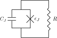
Figure 1: Resistively (and capacitively) shunted Josephson junction (RSJJ). The capacitance $C_{J}$ determines the charging energy $E_{C}=(2e)^{2}/2C_{J}$ of the junction while the transparency of the tunnel barrier and the superconducting gap set the Josephson coupling energy $E_{J}$.

We study the boundary sine-Gordon model (1) in the framework of the nonperturbative FRG [25, 26, 27], an approach which has proven very successful for the $(1+1)$-dimensional sine-Gordon model [28, 29]. We find that the transition is not controlled by a single fixed point but by a line of fixed points, and compute the continuously varying critical exponent $\nu$ associated with the relevant direction about the fixed point. These results qualitatively agree with the Monte Carlo simulations of Werner and Troyer (WT) who showed that the correlation function $\chi(\tau)=\langle e^{iq\varphi(\tau)}e^{-iq\varphi(0)}\rangle$ ($|q|\leq 1/2$) exhibits continuously varying critical exponents along the transition line [30, 31]. Recent NRG calculations also imply that the transition line is a line of fixed points [16]. Although no precise calculations are performed, we argue that the conductance varies continuously along the transition line.

Unlike the traditional phase diagram of the RSJJ, where the transition between the insulating and superconducting phases is located at $\alpha=1$, the FRG predicts the transition line in the plane $(\alpha,E_{J}/E_{C})$ to bend in the region $\alpha=R_{q}/R<1$. The FRG is however not reliable in the limit $\alpha\to 0$ since it predicts a phase transition at a finite value of $E_{J}/E_{C}$ while in the absence of dissipation the ground state of the model (1) is known to be insulating. This leads us to propose two possible scenarios for the Schmid transition. In the first one, the transition line is vertical and located at $\alpha=1$, as in the traditional phase diagram and in agreement with the Monte Carlo simulations of WT. In the second one, the transition line bends in the region $\alpha<1$, as in the FRG and NRG calculations [16, 17], but eventually the critical value of $E_{J}/E_{C}$ diverges as $\alpha\to 0$.

On the other hand we compute the phase mobility $\mu(\omega)$ (i.e. the mobility of the Brownian particle) related to the admittance $Y(\omega)=q^{2}/\mu(\omega)$ of the RSJJ. The dc mobility $\mu=\lim_{\omega\to 0}\mu(\omega)$ vanishes in the superconducting phase, and is equal to the mobility $\mu_{0}=2\pi/\alpha=1/\eta$ of the free particle in the insulating phase. The frequency dependence of the mobility in the superconducting phase is correctly obtained only for $\alpha\gtrsim 2$; when $1\leq\alpha\lesssim 2$, the FRG fails to capture the instantons connecting neighboring minima of the periodic potential. This does not prevent us to obtain the low-frequency behavior of the RSJJ; in the insulating phase $Y(\omega\to 0)=1/R$ whereas $Y(\omega)$ is purely inductive at low frequencies in the superconducting phase. However the effective inductance is not determined by the “coherence”, i.e. the expectation value $\langle\cos\varphi\rangle$, which in fact remains nonzero in the insulating phase. We compare our results for $\langle\cos\varphi\rangle$ and $\langle\cos(\varphi/2)\rangle$ with results obtained from integrability methods and Monte Carlo simulations [32, 31].

II FRG formalism.

Following the standard strategy of the nonperturbative functional renormalization group (FRG) we add to the action an infrared regulator term [25, 26, 27],

$$\Delta S_{k}[\varphi]=\frac{1}{2}\sum_{\omega_{n}}R_{k}(i\omega_{n})\varphi(-i\omega_{n})\varphi(i\omega_{n}),$$ (2)

which suppresses fluctuation modes whose frequency is smaller than the (running) frequency $k$, i.e. $|\omega_{n}|\lesssim k$, but leaves unaffected those with $|\omega_{n}|\gtrsim k$. The cutoff function is written in the form

$$R_{k}(i\omega_{n})=\frac{\alpha}{2\pi}|\omega_{n}|r\left(\frac{|\omega_{n}|}{k}\right)+Z_{2,k}\omega_{n}^{2}r\left(\frac{\omega_{n}^{2}}{k^{2}}\right),$$ (3)

where $Z_{2,k}=\frac{1}{2\pi}\int_{0}^{2\pi}d\phi\,Z_{2,k}(\phi)$ is the field average of the function $Z_{2,k}(\phi)$ defined in Eq. (8) and $r(x)=4(1-x)^{2}/x\,\Theta(1-x)$. Including the second term in (3) allows us to consider the limit $\alpha\to 0$. The partition function

$${\cal Z}_{k}[J]=\int{\cal D}[\varphi]\,e^{-S[\varphi]-\Delta S_{k}[\varphi]+\int_{0}^{\beta}d\tau\,J\varphi}$$ (4)

thus becomes $k$ dependent. The expectation value of the field is given by

$$\phi(\tau)=\frac{\delta\ln{\cal Z}_{k}[J]}{\delta J(\tau)}=\langle\varphi(\tau)\rangle.$$ (5)

The scale-dependent effective action

$$\Gamma_{k}[\phi]=-\ln{\cal Z}_{k}[J]+\int_{0}^{\beta}d\tau\,J\phi-\Delta S_{k}[\phi]$$ (6)

is defined as a slightly modified Legendre transform which includes the subtraction of $\Delta S_{k}[\phi]$. Assuming that for $k=k_{\rm in}$ the fluctuations are completely frozen by the term $\Delta S_{k_{\rm in}}$, which is the case when $k_{\rm in}\gg\min(W,E_{C})$, $\Gamma_{k_{\rm in}}[\phi]=S[\phi]$. On the other hand, the effective action of the original model (1) is given by $\Gamma_{k=0}[\phi]$ since $R_{k=0}$ vanishes. The nonperturbative FRG approach aims at determining $\Gamma_{k=0}$ from $\Gamma_{k_{\rm in}}$ using Wetterich’s equation [33, 34, 35]

$$\partial_{t}\Gamma_{k}[\phi]=\frac{1}{2}{\rm Tr}\Bigl{\{}\partial_{t}R_{k}\bigl{(}\Gamma_{k}^{(2)}[\phi]+R_{k}\bigr{)}^{-1}\Bigr{\}},$$ (7)

where $\Gamma_{k}^{(2)}$ is the second-order functional derivative of $\Gamma_{k}$ and $t=\ln(k/k_{\rm in})$ a (negative) RG “time”.

II.1 FE₂ expansion

In the frequency expansion to second order (FE₂) [36], the scale-dependent effective action is approximated by

$$\Gamma_{k}[\phi]={} \frac{Z_{1}}{2}\sum_{\omega_{n}}|\omega_{n}|\phi(-i\omega_{n})\phi(i\omega_{n})$$

$$+\int_{0}^{\beta}d\tau\left[\frac{1}{2}Z_{2,k}(\phi)({\partial_{\tau}}\phi)^{2}+U_{k}(\phi)\right]$$ (8)

with initial conditions

$$Z_{1}=\frac{\alpha}{2\pi},\quad Z_{2,k_{\rm in}}(\phi)=\frac{1}{2E_{C}},\quad U_{k_{\rm in}}(\phi)=-E_{J}\cos\phi.$$ (9)

The effective potential $U_{k}(\phi)$ is given by the effective action when the field $\phi(\tau)\equiv\phi$ is time independent: $\Gamma_{k}[\phi]=\beta U_{k}(\phi)$. We anticipate the fact that $Z_{1}$ is not renormalized and therefore remains equal to its initial value. The zeroth-order harmonic of $Z_{2,k}(\phi)$ and the first-order harmonic of $U_{k}(\phi)$ can be seen as renormalized values of the coupling constants $1/2E_{C}$ and $E_{J}$, respectively, but the flow equation generates higher-order harmonics.

In practice, one introduces the dimensionless quantities

$$\tilde{U}_{k}(\phi)=\frac{U_{k}(\phi)}{k},\qquad\tilde{Z}_{2,k}(\phi)=kZ_{2,k}(\phi),$$ (10)

which ensure that the zero-temperature quantum phase transition between the superconducting and insulating phases corresponds to a fixed point of the flow equations. The latter, which are given in Appendix A, must be solved numerically.

II.2 Mobility and admittance

In addition to the effective potential $U_{k}(\phi)$, whose RG flow indicates whether the RSJJ is insulating or superconducting, a fundamental quantity is the mobility $\mu(i\omega_{n})=|\omega_{n}|G(i\omega_{n})$ of the quantum Brownian particle, i.e. its average (long-time) velocity when it is subjected to an external force. Since the phase propagator $G_{k}(i\omega_{n},\phi)=1/\Gamma^{(2)}_{k}(i\omega_{n},\phi)$ is given by the inverse of the two-point vertex, whose most general expression reads $\Gamma_{k}^{(2)}(i\omega_{n},\phi)=Z_{1}|\omega_{n}|+\Delta_{k}(i\omega_{n},\phi)+U^{\prime\prime}_{k}(\phi)$ (for a time-independent field), the scale-dependent mobility reads

$$\mu_{k}(i\omega_{n})=\frac{|\omega_{n}|}{\frac{\alpha}{2\pi}|\omega_{n}|+\Delta_{k}(i\omega_{n},0)+U^{\prime\prime}_{k}(0)}.$$ (11)

We consider the vanishing field configuration $\phi=0$ since this corresponds to the minimum of the effective potential for any $k>0$. In the FE₂, the self-energy $\Delta_{k}$ is approximated by its lowest-order derivative expansion, i.e. $\Delta_{k}(i\omega_{n},\phi)=Z_{2,k}(\phi)\omega_{n}^{2}$. To obtain the frequency-dependent mobility $\mu(\omega)$ in real time, one must first take the limit $k\to 0$ and perform the analytic continuation $i\omega_{n}\to\omega+i0^{+}$; the dc mobility is then given by $\mu=\mu(\omega\to 0)$. In the FE₂, the determination of $\Delta_{k}(i\omega_{n},\phi)$ is however valid only in the limit $|\omega_{n}|\ll k$ —for the same reason that the derivative expansion in the $\varphi^{4}$ theory is valid only in the small-momentum limit $|{\bf p}|\ll k$ [27]— and setting $k\to 0$ followed by $\omega\to 0$ (or $\omega_{n}\to 0$) is not, at least in principle, possible. We shall see how Eq. (11) can nevertheless be used to obtain useful information about the mobility.

When the RSJJ is biased by an infinitesimal external time-dependent current $I(t)$, the mobility determines the induced voltage $V(t)$ across the junction [1], i.e. the admittance

$$Y(\omega)=\frac{I(\omega)}{V(\omega)}=\frac{q^{2}}{\mu(\omega)}$$ (12)

for a sinusoidal current.

III The Schmid transition

In this section, we discuss the phase diagram obtained from the FRG approach and the nature of the transition between the superconducting and insulating phases. We compare our findings with the traditional view of the SB transition and previous numerical results. We also comment on some differences with the FRG results of Masuki et al. [16, 17].

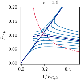
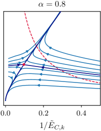
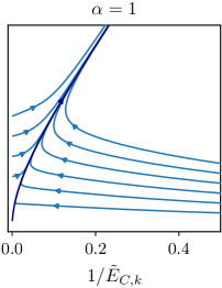
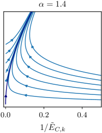
Figure 2: Flow diagram projected on the $(1/\tilde{E}_{C,k},\tilde{E}_{J,k}$) plane, where $1/2\tilde{E}_{C,k},$ and $\tilde{E}_{J,k}$ denote the zeroth- and first-order harmonics of $\tilde{Z}_{2,k}(\phi)$ and $\tilde{U}_{k}(\phi)$, respectively ($\alpha=0.6,0.8,1,1.4$ from left to right). The red point shows the fixed point obtained by solving $\partial_{k}\tilde{U}_{k}(\phi)=\partial_{k}\tilde{Z}_{2,k}(\phi)=0$. The red dashed lines, showing the effective initial conditions of the flow $(1/\tilde{E}_{C,W}=W/E_{C},\tilde{E}_{J,W}=E_{J}/W)$ at fixed $E_{J}/E_{C}=0.02$ when $W$ is varied [37], indicate that a smaller bandwidth $W$ favors the superconducting phase.

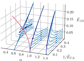
Figure 3: Flow diagram projected on the $(1/\tilde{E}_{C,k},\tilde{E}_{J,k})$ plane for $\alpha=0.6$, $1$ and $1.4$. The line of critical fixed points for $\alpha<1$ is shown in red.

III.1 Phase diagram

Typical flow trajectories, shown in Figs. 2 and 3, are in agreement with previous results by Masuki et al. [16, 17]. When $\alpha>1$, there is a (repulsive) trivial fixed point $\tilde{U}^{\prime}(\phi)=\tilde{Z}_{2}(\phi)=0$ and all RG trajectories with initial condition $\tilde{E}_{J,k_{\rm in}}=E_{J}/k_{\rm in}>0$ flow to the strong coupling limit where both the effective potential $\tilde{U}^{\prime}(\phi)$ and $\tilde{Z}_{2}(\phi)$ flow to infinity [38]: The system is in the superconducting phase. When $\alpha<1$, in addition to the trivial fixed point $\tilde{U}^{\prime}(\phi)=\tilde{Z}_{2}(\phi)=0$, which is now attractive, we find a critical fixed point $(\tilde{U}^{*}{}^{\prime}(\phi),\tilde{Z}_{2}^{*}(\phi))$, so that the trajectories can flow to either the trivial fixed point or the strong-coupling limit depending on the initial conditions at scale $k=k_{\rm in}$. Thus the system can be either superconducting ($\tilde{U}_{k}^{\prime},\tilde{Z}_{2,k}\to\infty$ for $k\to 0$) or insulating ($\tilde{U}_{k}^{\prime},\tilde{Z}_{2,k}\to 0$).

The location of the critical fixed point as $\alpha$ varies can be obtained by solving the equations $\partial_{k}\tilde{U}_{k}^{\prime}(\phi)=\partial_{k}\tilde{Z}_{2,k}(\phi)=0$ (Fig. 4). When $\alpha\to 0$, the action (1) corresponds to the one-dimensional sine-Gordon model and describes a frictionless quantum particle in a one-dimensional periodic potential. Since all quantum states of the particle are extended, the ground state should be insulating in that limit, whatever the value of $E_{C}$ and $E_{J}$. The existence of a fixed point at a finite value $\tilde{E}_{J}^{*}/\tilde{E}_{C}^{*}$ when $\alpha=0$ is a known artifact of the FRG-FE₂ approach to the one-dimensional sine-Gordon model [39]. In the limit $\alpha\to 0$, we expect the fixed point (shown by a red dot in Fig. 4) to move to infinity, i.e. $\tilde{E}_{J}^{*}/\tilde{E}_{C}^{*}\to\infty$ [40].

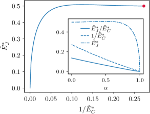
Figure 4: Location of the critical fixed point in the plane $(1/\tilde{E}_{C}^{*},\tilde{E}_{J}^{*})$ as $\alpha$ varies. The inset shows $1/\tilde{E}_{C}^{*}$ and $\tilde{E}_{J}^{*}$ vs $\alpha$. Near $\alpha=1$, $1/\tilde{E}_{C}^{*}\sim 1-\alpha$ and $\tilde{E}_{J}^{*}\sim\sqrt{1-\alpha}$. The red point shows the (spurious) fixed point obtained when $\alpha=0$ (see text for a discussion).

The phase diagram as a function of the bare parameters of the model is shown in Fig. 5. We find a transition between an insulating and a superconducting phase in the region $\alpha<1$. In the large bandwidth limit $W/E_{C}\gg 1$, the transition line depends only on the ratio $E_{J}/E_{C}$ and starts with an infinite slope: $(E_{J}/E_{C})_{\rm crit}\sim(1-\alpha)^{0.5}$ when $\alpha\to 1^{-}$. The transition line then bends towards the region $\alpha<1$, a direct consequence of the existence of the line of critical fixed points shown in Fig. 4. The finite value of $(E_{J}/E_{C})_{\rm crit}$ in the limit $\alpha\to 0$ is due to $\tilde{E}_{J}^{*}$ remaining finite; if $\tilde{E}_{J}^{*}\to\infty$ when $\alpha\to 0$ (as it should be, see the previous discussion) the RSJJ is insulating whatever the value of the Josephson energy $E_{J}$. Two possible scenarios are shown in Fig. 5 (bottom panel). The first one is a vertical transition line located at $\alpha=1$, as in the traditional picture of the Schmid transition and in agreement with the Monte Carlo simulations of WT in the large bandwidth limit $W\gg E_{C}$ who find that the transition occurs at $\alpha=1.00(2)$ at least up to $E_{J}/E_{C}\sim 0.5$ [30, 41]. In this scenario, the presence of the spurious fixed point at $\alpha=0$ invalidates the entire transition line obtained in the FE₂, the only vestige of the true transition line being the vertical tangent at $\alpha=1$. In the second scenario, the spurious fixed point at $\alpha=0$ invalidates the FE₂ result for $\alpha\ll 1$ but the obtained transition line is correct in a finite interval near $\alpha=1$. The NRG results of Masuki et al. [16] also yield a transition line that bends in the region $\alpha<1$ but with two qualitative differences with the FRG results reported here: The transition line exhibits a vanishing slope near $\alpha=1$ and a reentrance of the superconducting phase at small $\alpha$ (which is hard to reconcile with the known phase diagram of the one-dimensional sine-Gordon model ($\alpha=0$), see the discussion above).

Moving away from the large bandwidth limit, at fixed $E_{C}$, favors the superconducting phase as shown in Fig. 2: Decreasing $W$ will always change the initial conditions of the flow so as to make the system superconducting. Thus $(E_{J}/E_{C})_{\rm crit}$ decreases when $W$ is lowered. As shown in the inset of Fig. 5, we find that the transition persists in the limit $W/E_{C}\to 0$ since $(E_{J}/W)_{\rm crit}$ remains finite. This differs from the conclusion of Ref. [16] that a nonzero value of $1/E_{C}$ is necessary to have a transition for $\alpha<1$.

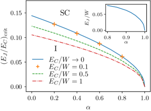
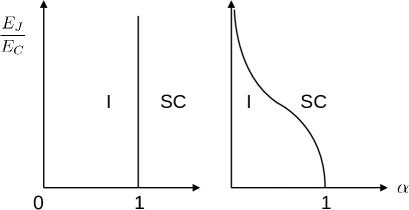
Figure 5: (Top) Zero-temperature phase diagram of the RSJJ as a function of the bare parameters of the model ($\alpha$, $E_{J}$, $1/E_{C}$ and $W$) showing the insulating (I) and superconducting (SC) phases. The transition line depends only on the ratio $E_{J}/E_{C}$ when $W\gg E_{C}$. The inset shows the phase diagram for $W/E_{C}=0.01$. As explained in the text, the existence of a transition at a finite value $(E_{J}/E_{C})_{\rm crit}$ when $\alpha\to 0$ is an artifact of the FE₂. (Bottom) Two possible scenarios for the Schmid transition taking into account the absence of transition in the limit $\alpha\to 0$.

III.2 Critical behavior

III.2.1 Critical exponent $\nu$

The functions $\tilde{U}^{*}{}^{\prime}(\phi)$ and $\tilde{Z}^{*}_{2}(\phi)$ at the fixed point controlling the phase transition are shown in Fig. 6 for $\alpha=0.8$. The RG eigenvalue $1/\nu$ associated with the relevant perturbation, shown in Fig 7, is determined by linearizing the flow about the fixed point.

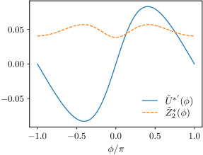
Figure 6: Fixed-point functions $\tilde{U}^{*}{}^{\prime}(\phi)$ and $\tilde{Z}^{*}_{2}(\phi)$ for $\alpha=0.8$.

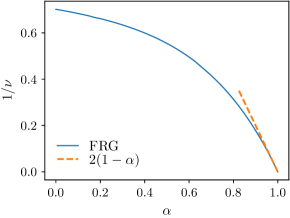
Figure 7: Critical exponent $\nu$ vs $\alpha$. The dashed (red) line shows the result $1/\nu=2(1-\alpha)$ valid near $\alpha=1$.

Near $\alpha=1$, the critical fixed point is close to the Gaussian fixed point and can be analyzed from perturbation theory. We use the harmonic expansion $\tilde{U}_{k}(\phi)=\sum_{n=0}^{\infty}\tilde{u}_{n,k}\cos(n\phi)$ and $\tilde{Z}_{2k}(\phi)=\sum_{n=0}^{\infty}\tilde{z}_{n,k}\cos(n\phi)$, and expand the flow equations in powers of $\epsilon=1-1/\alpha$. When $\epsilon\to 0$, the flow of $\tilde{u}_{1,k}$ is initially much slower than the flow of all other coupling constants. After a transient regime, the values of $\tilde{u}_{n\neq 1,k}$ and $\tilde{z}_{n,k}$ are determined by $\tilde{u}_{1,k}$ alone and all RG trajectories collapse on a single line, as shown in Figs. 2 and 3 for the trajectories projected on the plane $(\tilde{z}_{0},\tilde{u}_{1})$. The flow along this line is determined by the beta function

$$\partial_{t}\tilde{u}_{1,k}=\left(\frac{1}{\alpha}-1\right)\tilde{u}_{1,k}+{\cal F}\tilde{u}_{1,k}^{3},$$ (13)

where ${\cal F}$ is a complicated combination of threshold functions (see Appendix B for detail). Note that this beta function is not exact (to order $\tilde{u}^{3}_{1,k}$) since it relies on the FE₂ expansion.

Linearizing the flow equation (13) about its nontrivial fixed point $\tilde{u}_{1}^{*}=[(\alpha-1)/\alpha{\cal F}]^{1/2}$ yields the critical exponent $1/\nu=2(1-\alpha)+{\cal O}((1-\alpha)^{2})$, regardless of the value of ${\cal F}$. Only the sign of ${\cal F}$ matters (assuming ${\cal F}$ to be nonzero) since it determines whether the fixed point $\tilde{u}_{1}^{*}$ exists when $\alpha<1$ or $\alpha>1$. The fixed point is repulsive if $\alpha<1$ ($1/\nu>0$) and attractive if $\alpha>1$ ($1/\nu<0$), in agreement with the trivial fixed point $\tilde{u}_{1}=0$ being attractive if $\alpha<1$ and repulsive if $\alpha>1$. A numerical evaluation yields ${\cal F}<0$ thus indicating that the nontrivial fixed point exists when $\alpha<1$.

In their Monte Carlo simulations [30], WT also observed that the transition is not controlled by a single fixed point, but rather by a line of critical points: By considering the correlation function $\langle e^{iq\varphi(\tau)}e^{-iq\varphi(0)}\rangle$ ($|q|\leq 1/2$), they obtained continuously varying exponents along the transition line, in full agreement with the FRG analysis, see Sec. III.2.2.The NRG calculations of Masuki et al. also predict the Schmid transition to be controlled by a line of fixed points [16].

The bending of the transition line in the region $\alpha<1$ clearly simplifies the study of the critical behavior. For a vertical transition line at $\alpha=1$, one would expect the cubic term ${\cal F}$ and all higher-order terms in the beta function (13) to vanish, in order to ensure that the transition line is a fixed line. There are various claims in the literature that the cubic term ${\cal F}$ in the beta function vanishes although no detailed calculations seem to have been reported [5, 6]. Interestingly, a nonzero cubic term was found by Bulgadaev in his original paper [4]. In the FE₂ expansion, the vanishing of the beta function to all orders at $\alpha=1$ is made impossible by the (spurious) fixed point at $\alpha=0$, which is at the origin of the transition line in the region $\alpha<1$.

Note that in the scenario where the line of fixed points and the transition line are vertical, $1/\nu$ vanishes since the beta function $\partial_{t}\tilde{u}_{1,k}=(1/\alpha-1)\tilde{u}_{1,k}$ is identically zero for $\alpha=1$. The situation is different for the exponent $\gamma$ discussed in the following section.

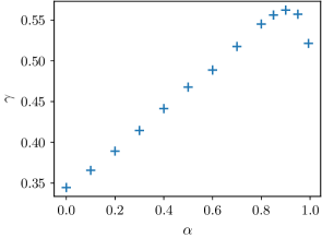
Figure 8: Critical exponent $\gamma$ associated with the correlation function $\chi(\tau)$ [Eq. (14)].

III.2.2 Correlation function $\langle e^{\frac{i}{2}\varphi(\tau)}e^{-\frac{i}{2}\varphi(0)}\rangle$

Following WT [30, 31], we consider the correlation function

$$\chi(\tau)=\langle e^{\frac{i}{2}\varphi(\tau)}e^{-\frac{i}{2}\varphi(0)}\rangle.$$ (14)

The computation of its Fourier transform $\chi_{k}(i\omega_{n})$ for $i\omega_{n}=0$ is discussed in Appendix C. At criticality we find that $\chi_{k}(i\omega_{n}=0)\sim 1/k^{1-\gamma}$ diverges with some exponent $1-\gamma$. By dimensional analysis, we then obtain $\chi_{k=0}(i\omega_{n})\sim 1/|\omega_{n}|^{1-\gamma}$ and

$$\chi_{k=0}(\tau)\sim\frac{1}{|\tau|^{\gamma}}.$$ (15)

The exponent $\gamma$ is shown in Fig. 8. The limiting value $\gamma\simeq 0.5$ when $\alpha\to 1$ (i.e. $E_{J}\to 0$) agrees with the result of Lukyanov and Werner obtained from integrability methods [31]. We note however that $\gamma$ exhibits a maximum for $\alpha\sim 0.9$ while they obtain a strictly monotonous exponent along the transition line.

The qualitative agreement between our results and those of Lukyanov and Werner (except for the maximum near $\alpha\sim 0.9$) suggests that our determination of the exponent $\gamma$ along the transition line is correct even in the scenario where the transition line is vertical.

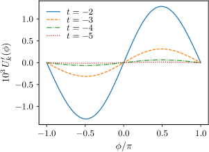
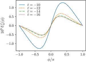
Figure 9: $U_{k}^{\prime}(\phi)=k\tilde{U}^{\prime}_{k}(\phi)$ vs $t=\ln k$ in the insulating (top) and superconducting (bottom) phases. $E_{*}=\lim_{k\to 0}U^{\prime\prime}_{k}(0)$ vanishes in the former case but is finite in the latter as shown in Fig. 10. [$E_{J}=10^{-2}E_{C}$, $W\to\infty$, $\alpha=0.6$ (top) $\alpha=1.4$ (bottom).]

III.2.3 Mobility and conductance

At the fixed point, $Z_{2,k}(\phi)=\tilde{Z}_{2,k}(\phi)/k\to\tilde{Z}_{2}^{*}(\phi)/k$ for $k\to 0$ whereas $U_{k}(\phi)=k\tilde{U}_{k}(\phi)\to 0$. The divergence of $Z_{2,k}(\phi)$ is not a problem since $Z_{2,k}(\phi)\omega_{n}^{2}$ remains finite in the domain of validity of the FE₂ ($|\omega_{n}|\ll k$). It indicates however that the $\omega_{n}^{2}$ dependence of the self-energy $\Delta_{k}(i\omega_{n},\phi)$ is not preserved by the RG flow in the regime $k\ll|\omega_{n}|$ and one expects $\Delta_{k=0}(i\omega_{n},\phi)\sim|\omega_{n}|$ at low energies. Heuristically one can obtain this result by stopping the flow of $Z_{2,k}(\phi)$ at $k\sim|\omega_{n}|$ since one expects $\omega_{n}$ to play the role of an infrared cutoff when computing the two-point vertex $\Gamma^{(2)}_{k}(i\omega_{n},\phi)$. Assuming $\Delta_{k=0}(i\omega_{n},0)=C|\omega_{n}|$, with $C$ a function of $\alpha$, one then deduces from (11) that at the Schmid transition the dc mobility

$$\mu=\frac{1}{\frac{\alpha}{2\pi}+C}$$ (16)

takes a nontrivial (i.e. different from 0 and $2\pi/\alpha$) value that depends only on $\alpha$. As a result, the dc conductance ${\cal G}=q^{2}/\mu$ also takes a nontrivial value. The FE₂ does not allow us to determine the value of the $\alpha$-dependent constant $C$ but a more refined approximation scheme, e.g. the Blaizot–Mendez-Galain–Wschebor approximation [42, 43, 44], would yield the whole frequency dependence of the self-energy (regardless of the value of $|\omega_{n}|/k$) and thus the mobility $\mu$ and conductance ${\cal G}$ along the transition line.

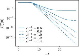
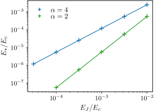
Figure 10: (Top) $U^{\prime\prime}_{k}(0)$ vs $t=\ln k$ for various values of $\alpha$ and $E_{J}=0.01$, $1/E_{C}=0.02$. $E_{*}=\lim_{k\to 0}U^{\prime\prime}_{k}(0)$ takes a nonzero value in the superconducting phase. (Bottom) $E_{*}$ vs $E_{J}$ in the superconducting phase. The solid lines show the power law behavior $E_{*}\sim E_{J}^{\alpha/(\alpha-1)}$.

IV Superconducting and insulating phases

In this section, we compute various observables in order to characterize the insulating and superconducting phases, and compare, when possible, with known results obtained from integrability methods and Monte Carlo simulations.

IV.1 RG flows

Figure 9 shows the flow of the function $U_{k}^{\prime}=k\tilde{U}_{k}^{\prime}$ in the insulating and superconducting phases. Although $U^{\prime}_{k=0}(\phi)=0$, as imposed by the periodicity and convexity of the effective potential [45], the behavior near $\phi=0$ is markedly different in each phase. In the insulating phase, $U^{\prime}_{k}(\phi)$ decreases with $k$ and $U_{k}^{\prime\prime}(\phi)\to 0$ for all $\phi$. On the other hand, in the superconducting phase $U^{\prime\prime}_{k}(\phi)$ reaches a nonzero value in the neighborhood of $\phi=0$. Although this neighborhood shrinks as $k\to 0$, this implies that $E_{*}=\lim_{k\to 0}U_{k}^{\prime\prime}(0)$ takes a nonzero value (Fig. 10); $U^{\prime\prime}_{k}(\phi)$ converges non-uniformally towards $U^{\prime\prime}_{k=0}(\phi)=0$ [46]. We conclude that the characteristic energy scale $E_{*}$ vanishes in the insulating phase but is nonzero in the superconducting phase where it varies as

$$E_{*}\sim E_{C}\left(\frac{E_{J}}{E_{C}}\right)^{\alpha/(\alpha-1)}$$ (17)

in the large bandwidth limit $W\gg E_{C}$, as shown in Fig. 10. When approaching the transition, $E_{*}$ vanishes with the exponent $\nu$, i.e. $E_{*}\sim(E_{J}-E_{J}^{(c)})^{\nu}$ if $E_{J}$ is varied at fixed $E_{C}$ (see Fig. 13).

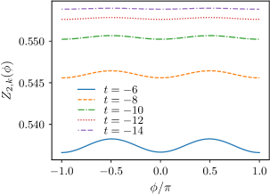
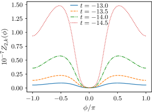
Figure 11: $Z_{2,k}(\phi)$ vs $t=\ln k$ in the insulating (top) and superconducting (bottom) phases. [$E_{J}=10^{-2}E_{C}$, $W\to\infty$, $\alpha=0.6$ (top) $\alpha=1.4$ (bottom)]

The function $Z_{2,k}(\phi)$ is shown in Fig. 11. While in the insulating phase $Z_{2,k}(\phi)$ becomes constant for $k\to 0$, in the superconducting phase it is strongly non-monotonous, with a form that is reminiscent of the $(1+1)$-dimensional sine-Gordon model [28], and takes large values. At intermediate stages of the flow, when $k\gg E_{*}$, we find that $-\partial_{t}\ln Z_{2,k}(0)\simeq 3-2/\alpha$ takes a $k$-independent value (Fig. 12), which indicates that the self-energy behaves as $\Delta_{k=0}(i\omega_{n})\sim|\omega_{n}|^{2/\alpha-1}$ when $|\omega_{n}|\gg E_{*}$. The flow of $Z_{2,k}(\phi)$ however always stops when $k\ll E_{*}$ and $Z_{2,k}(\phi)$ reaches a nonzero value, implying that the self-energy $\Delta_{k=0}(i\omega_{n},\phi)\sim\omega_{n}^{2}$ is a quadratic function of the frequency for $\omega_{n}\to 0$ (as in the insulating phase).

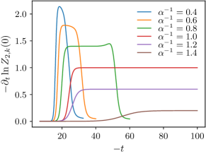
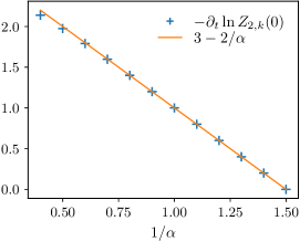
Figure 12: (Top) $-\partial_{t}\ln Z_{2,k}(0)$ vs $t=\ln k$. (Bottom) The value of $-\partial_{t}\ln Z_{2,k}(0)$ on the plateau (as shown in the top panel) vs $\alpha$. The system is in the superconducting phase for $\alpha\geq 1$, and in the insulating phase otherwise. [$E_{J}/E_{C}=2\cdot 10^{-5}$, $W\to\infty$.]

These results imply that the propagator can be written in the form

$$G_{k=0}(i\omega_{n})=\frac{1}{\frac{\alpha}{2\pi}|\omega_{n}|+E_{*}}$$ (18)

in the low-energy limit (neglecting the $\omega_{n}^{2}$ term). In the insulating phase the propagator $G_{k=0}$ is field independent whereas Eq. (18) holds for $\phi=0$ in the superconducting phase. Equation (18) is correct in the insulating phase (where $E_{*}=0$) and in the superconducting phase when $\alpha\gtrsim 2$; in the latter case the physics is dominated by small fluctuations of the phase about the minima of the periodic potential $-E_{J}\cos(\varphi)$. On the other hand, Equation (18) is not correct when $1\leq\alpha\lesssim 2$, a regime where transitions between neighboring minima (instantons) play a crucial role [47].

IV.2 Mobility and admittance

The real part of the mobility $\mu(\omega)=\mu^{\prime}(\omega)+i\mu^{\prime\prime}(\omega)$ is deduced from (18),

$$\mu^{\prime}(\omega)=\frac{\alpha}{2\pi}\frac{\omega^{2}}{\bigl{(}\frac{\alpha}{2\pi}\omega\bigr{)}^{2}+E^{2}_{*}}.$$ (19)

Thus the dc mobility $\mu(\omega=0)$ is equal to $2\pi/\alpha=\mu_{0}$ in the insulating phase and vanishes in the superconducting phase (Fig. 13). However, the expression of the propagator (18) being incorrect when $1\leq\alpha\lesssim 2$, the frequency dependence of the mobility (19) is not correct in this regime and should vanish as

$$\mu^{\prime}(\omega)\sim|\omega|^{2\alpha-2}$$ (20)

when $\omega\to 0$ [48, 49, 50]. The behavior of the self-energy, $\Delta_{k}(i\omega_{n})\sim|\omega_{n}|^{2/\alpha-1}$, in the frequency range $|\omega_{n}|\gg E_{*}$ allows us to recover the perturbative (high-frequency) expansion of the mobility $\mu^{\prime}(\omega)=\mu_{0}-{\rm const}\,|\omega|^{2/\alpha-2}$ [23], but the FE₂ expansion fails to reproduce the low-energy behavior (20).

From (12), we deduce the low-frequency behavior of the admittance [51]

$$Y(\omega)=\left\{\begin{array}[]{ll}\dfrac{1}{R}&\mbox{ (I)},\\ \dfrac{1}{R}+\dfrac{i}{L_{\rm eff}(\omega+i0^{+})}&\mbox{ (SC)}.\end{array}\right.$$ (21)

Thus the junction has a vanishing transmission in the insulating phase (I) —the whole current flowing through the resistor— and behaves as an effective inductance $L_{\rm eff}=1/q^{2}E_{*}$ in the superconducting phase (SC). At the beginning of the flow (i.e. at the classical level), where $U_{k_{\rm in}}(\phi)=-E_{J}\cos\phi$, one finds the expected result $1/L_{{\rm eff},k_{\rm in}}=q^{2}U^{\prime\prime}_{k_{\rm in}}(0)=q^{2}E_{J}$. Note that the inductive response in the superconductive phase follows solely from the vanishing of the self-energy for $\omega_{n}\to 0$, i.e. $\Delta_{k}(i\omega_{n}=0,\phi)=0$. The value of $E_{*}=\lim_{k\to 0}U^{\prime\prime}_{k}(0)$, and whether it vanishes or not, however requires to solve the FRG flow equations.

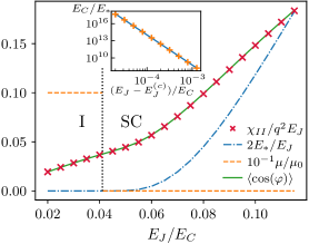
Figure 13: Energy scale $E_{*}$, dc mobility $\mu=\mu(\omega=0)$, coherence $\langle\cos\varphi\rangle$ and current-current correlation function $\chi^{R}_{II}(0)$ vs $E_{J}$ in the large bandwidth limit $W/E_{C}\to\infty$ for $\alpha\simeq 0.909$. The transition, indicated by the black dotted vertical line, occurs for $E_{J}^{(c)}/E_{C}\simeq 0.0432$. The inset shows the divergence of $1/E_{*}$ in the superconducting phase as the transition is approached. The blue line is a fit $1/E_{*}\sim(E_{J}-E_{J}^{(c)})^{-\nu}$ with the exponent $\nu\simeq 5.3$ obtained from the linearized flow equations (Fig. 4, bottom panel).

IV.3 Coherence and current-current correlation function

The expectation value $\langle\cos\varphi\rangle$ is computed by adding to the action a time-independent external complex source $h$. The effective potential $U_{k}(\phi,h^{*},h)$ is then a function of $\phi$, $h^{*}$ and $h$ and $\langle\cos\varphi\rangle=-U^{(1,0)}(0)$ where $U^{(1,0)}(\phi)=\partial_{h^{*}}U(\phi,h^{*},h)|_{h^{*}=h=0}$ (see Appendix C for details). Contrary to the NRG result of Ref. [16], we find that the coherence $\langle\cos\varphi\rangle$ never vanishes, although it becomes very small in the insulating phase (see the inset in Fig. 14), and does not allow one to discriminate between the superconducting and insulating ground states of the RSJJ (Fig. 13). One cannot discard the possibility that a more accurate description of the superconducting phase in the range $1\leq\alpha\lesssim 2$, taking into account the instantons connecting neighboring minima of the periodic potential (see the discussion at the end of the previous section), would give a vanishing coherence in the neighboring of $\alpha=1$, but such a scenario seems rather unlikely.

If we expand the potential $U^{(1,0)}(\phi)=\sum_{n=0}^{\infty}u_{n}^{(1,0)}\cos(n\phi)$ in circular harmonics, we observe that in the insulating phase (where we would naively expect the coherence to vanish since the effective potential is irrelevant), the nonzero value of $U^{(1,0)}(0)$ is entirely due to the zeroth-order harmonic amplitude $u_{0}^{(1,0)}$ so that the nonzero value of the coherence comes from the dependence of the free energy on the external source $h$. Even though the Josephson coupling is irrelevant in the insulating phase, the coherence cannot be simply computed from the Gaussian action obtained by setting $E_{J}=0$ (in which case one would find $\langle\cos\varphi\rangle=0$), we must keep track of the contribution of the high-energy modes to the free energy and its dependence on the external source $h$.

Because of the U(1) invariance of the action (1), i.e. the invariance in the shift $\varphi(\tau)\to\varphi(\tau)+a$ of the field by an arbitrary constant, the coherence is related to the current-current correlation function $\chi^{R}_{II}(\omega)$ (with $I=qE_{J}\sin\varphi$ the current through the junction) by [52]

$$q^{2}E_{J}\langle\cos\varphi\rangle-\chi^{R}_{II}(\omega=0)=0,$$ (22)

which is the analog of the $f$-sum rule in electron systems with $q^{2}E_{J}\langle\cos\varphi\rangle$ playing the role of the diamagnetic term. This relation is well satisfied by the FRG results (Fig. 13).

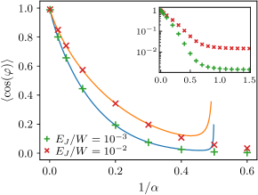
Figure 14: Expectation value $\langle\cos\varphi\rangle$ vs $\alpha$ in the superconducting phase when $1/E_{C}=0$. The lines show the exact result obtained from integrability methods [32].

The free energy $f=-\frac{1}{\beta}\ln{\cal Z}$ of the boundary sine-Gordon model is known exactly in the superconducting phase when $\alpha>2$ and $1/E_{C}=0$ [32]. Using $\langle\cos\varphi\rangle=-\partial f/\partial E_{J}$, one obtains

$$\langle\cos\varphi\rangle=\frac{\Gamma\left(\frac{\alpha-2}{2\alpha-2}\right)\Gamma\left(\frac{1}{2\alpha-2}\right)}{2\pi^{3/2}\left(1-\frac{1}{\alpha}\right)\frac{E_{J}}{2bW}}\left(\frac{\pi E_{J}}{2bW\Gamma(1/\alpha)}\right)^{\alpha/(\alpha-1)}.$$ (23)

Note that a finite UV cutoff $W$ is necessary to make the boundary sine-Gordon model well defined when $1/E_{C}=0$. $b$ is a scale factor depending on the implementation of the UV cutoff; for a hard cutoff, $b=e^{\gamma}/2$ with $\gamma$ the Euler constant [28]. Figure 14 shows that the FRG reproduces the exact result (23) with a very good accuracy.

Finally we discuss the expectation value $\langle\cos(\varphi/2)\rangle$, whose exact expression has been conjectured by Fateev et al. in the case $1/E_{C}=0$ and $W<\infty$ (see Eq. (3) in Ref. [32]). It has also been computed by Lukyanov and Werner in the case $1/E_{C}>0$ and $W\to\infty$ [31]. Figure 15 shows a comparison with the FRG results. In both cases ($1/E_{C}=0$, $W<\infty$ and $1/E_{C}>0$, $W\to\infty$), there is a good agreement for $\alpha\gtrsim 2$, which shows that the FE₂ is fully (quantitatively) reliable for these values of $\alpha$. However the agreement deteriorates as $\alpha$ approaches one, again a sign that the FE₂ is not reliable in the range $1\leq\alpha\lesssim 2$.

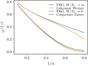
Figure 15: Expectation value $\langle\cos(\varphi/2)\rangle$ in the superconducting phase obtained from the FRG and compared with the conjecture of Fateev et al. [32] in the case $1/E_{C}=0$, $W<\infty$, and the Monte Carlo simulations of Lukyanov and Werner [31] in the case $1/E_{C}>0$, $W\to\infty$.

V Conclusion

Our FRG study of the RSJJ has met with mixed success. On the one hand, it clearly shows that the Schmid transition is not controlled by a single fixed point but by a line of critical fixed points, in agreement with the conclusions of Werner, Troyer and Lukyanov based on Monte Carlo simulations and integrability methods [30, 31]. The same conclusion can be drawn from the NRG calculations of Masuki et al. [16].

On the other hand there are strong discrepancies regarding the location of the transition line in the plane $(\alpha,E_{J}/E_{C})$. In the large bandwidth limit $W/E_{C}\gg 1$, Werner and Troyer find a vertical line located at $\alpha=1$ with an accuracy of 2% (so that the transition can only be induced by varying $\alpha$), the NRG indicates that the transition line is curved in the region $\alpha<1$ in a concave way (except for a surprising reentrance of the superconducting phase at small $\alpha$), whereas the FRG gives a convex transition line which starts with an infinite slope at $\alpha=1$. As already pointed out, the FRG fails in the limit $\alpha\to 0$ and its prediction for the location of the transition line may not be reliable even in the vicinity of $\alpha=1$. These disagreements clearly call for further studies, in particular numerical. The FRG also fails to capture the correct frequency dependence of the mobility in the superconducting phase when $1\leq\alpha\lesssim 2$.

These two shortcomings —the spurious phase transition at $\alpha=0$ and the inability to capture the frequency dependence of the mobility when $1\leq\alpha\lesssim 2$— can be ascribed to the failure of the FRG in describing the instantons between neighboring minima of the periodic potential. This is in sharp contrast with the $(1+1)$ sine-Gordon model where a derivative expansion of the effective action to second order is sufficient to compute the mass of the solitons and the lowest-lying breather (soliton-antisoliton bound state) with high accuracy [28]. The description of topological defects is an open issue in the FRG approach. Aside from the topological excitations of the $(1+1)$-dimensional sine-Gordon model, the FRG provides us with a good description of the vortices and the Berezinskii-Kosterlitz-Thouless transition in the two-dimensional O(2) model [53, 54, 55], but a good description of the kinks in the one-dimensional Ising has still not been achieved [56, 57]. Whether or not the FRG approach, used here in combination with a second-order frequency expansion, can be improved in order to describe the instantons of the boundary sine-Gordon model is an open issue.

The discrepancies between the various theoretical and numerical approaches could in principle be settled by future experiments. By determining the location of the transition line one could distinguish between the two scenarios proposed in Fig. 5. We have provided a detailed prediction of this location near $\alpha=1$, as a function of $W$ and $E_{C}$, in the scenario where the transition line bends in the region $\alpha<1$ (top panel in Fig. 5), which could be checked in finite-frequency measurements of a RSJJ [12, 15].

Appendix A Flow equations

The flow equations of $U_{k}(\phi)$ and $Z_{2,k}(\phi)$ are obtained by relating these two quantities to the two-point vertex

$$\Gamma_{k}^{(2)}(i\omega_{n},\phi)=Z_{1}|\omega_{n}|+Z_{2,k}(\phi)\omega_{n}^{2}+U_{k}^{\prime\prime}(\phi)$$ (24)

in a time-independent field $\phi(\tau)=\phi$. Thus we have

$$\begin{split}\partial_{t}U_{k}^{\prime\prime}(\phi)&=\partial_{t}\Gamma_{k}^{(2)}(0,\phi),\\ \partial_{t}Z_{2,k}(\phi)&=\partial_{t}\frac{\Gamma_{k}^{(2)}(i\omega_{1},\phi)-\Gamma_{k}(0,\phi)}{\omega_{1}^{2}}\end{split}$$ (25)

where $\omega_{1}=2\pi T$ and we use a discrete frequency derivative for $Z_{2,k}(\phi)$. $\Gamma_{k}^{(2)}$ satisfies the flow equation

$$\partial_{t}\Gamma_{k}^{(2)}(i\omega_{\nu},\phi)={} \sum_{\omega_{n}}\partial_{t}R_{k}(i\omega_{n})\biggl{\{}-\frac{1}{2}G_{k}(i\omega_{n},\phi)^{2}\Gamma_{k}^{(4)}(i\omega_{\nu},-i\omega_{\nu},i\omega_{n},-i\omega_{n},\phi)$$

$$+G_{k}(i\omega_{n},\phi)^{2}\Gamma_{k}^{(3)}(i\omega_{\nu},i\omega_{n},-i\omega_{n+\nu},\phi)G_{k}(i\omega_{n+\nu},\phi)\Gamma_{k}^{(3)}(-i\omega_{\nu},i\omega_{n+\nu},-i\omega_{n},\phi)\biggr{\}},$$ (26)

where all quantities are evaluated in a time-independent field $\phi$. In the limit $T\to 0$, the Matsubara frequency becomes a continuous variable and the discrete sums can be replaced by integrals. Likewise the discrete derivative in (25) becomes a standard derivative. However, the propagator $G_{k}(i\omega_{n})$ being a non-analytic function of $\omega_{n}$, care must be taken when taking the derivative wrt $\omega_{\nu}^{2}$ of the rhs of (26) since a naive expansion in $\omega_{\nu}$ of the integrand may give wrong results [58, 59].

The flow equations for the dimensionless functions defined in (10) read

$$\partial_{t}\tilde{U}^{\prime\prime}_{k}={} -\tilde{U}^{\prime\prime}_{k}+2l_{2}^{3}\tilde{U}_{k}^{\prime\prime\prime}\tilde{Z}_{2,k}^{\prime}+l_{0}^{3}\tilde{U}^{\prime\prime\prime}_{k}{}^{2}-\frac{1}{2}l_{0}^{2}\tilde{U}^{(4)}_{k}+l_{4}^{3}\tilde{Z}_{2,k}^{\prime}{}^{2}-\frac{1}{2}l_{2}^{2}\tilde{Z}_{2,k}^{\prime\prime},$$ (27)

$$\partial_{t}\tilde{Z}_{2,k}={} \tilde{Z}_{2,k}+\frac{1}{2\tilde{\omega}_{1}^{2}}\Bigl{\{}2l_{0}^{2,1}(i\tilde{\omega}_{1})[\tilde{U}_{k}^{\prime\prime\prime}+\tilde{\omega}_{1}^{2}\tilde{Z}_{2,k}^{\prime}]^{2}+4\tilde{\omega}_{1}l_{1}^{2,1}(i\tilde{\omega}_{1})\tilde{U}_{k}^{\prime\prime\prime}\tilde{Z}_{2,k}^{\prime}+4l_{2}^{2,1}(i\tilde{\omega}_{1})\tilde{U}_{k}^{\prime\prime\prime}\tilde{Z}_{2,k}^{\prime}-4l_{2}^{3}\tilde{U}_{k}^{\prime\prime\prime}\tilde{Z}_{2,k}^{\prime}-2l_{0}^{3}\tilde{U}_{k}^{\prime\prime\prime}{}^{2}$$

$$+4\tilde{\omega}_{1}^{3}l_{1}^{2,1}(i\tilde{\omega}_{1})\tilde{Z}_{2,k}^{\prime}{}^{2}+6\tilde{\omega}_{1}^{2}l_{2}^{2,1}(i\tilde{\omega}_{1})\tilde{Z}_{2,k}^{\prime}{}^{2}-l_{0}^{2}\tilde{\omega}_{1}^{2}\tilde{Z}_{2,k}^{\prime\prime}+4\tilde{\omega}_{1}l_{3}^{2,1}(i\tilde{\omega}_{1})\tilde{Z}_{2,k}^{\prime}{}^{2}+2l_{4}^{2,1}(i\tilde{\omega}_{1})\tilde{Z}_{2,k}^{\prime}{}^{2}-2l_{4}^{3}\tilde{Z}_{2,k}^{\prime}{}^{2}\Bigr{\}},$$ (28)

where $\tilde{\omega}_{n}=\omega_{n}/k=2\pi n\tilde{T}$ with $\tilde{T}=1/\tilde{\beta}=T/k$ the dimensionless temperature. The prime, double prime, etc., denote derivatives wrt $\phi$. We have introduced the threshold functions

$$\begin{split}l_{p}^{m}={}&\frac{1}{\tilde{\beta}}\sum_{{\tilde{\omega}_{n}}}\dot{\tilde{R}}_{k}(i{\tilde{\omega}_{n}})\tilde{G}_{k}(i{\tilde{\omega}_{n}},\phi)^{m}|{\tilde{\omega}_{n}}|^{p},\\ l_{p}^{m_{1},m_{2}}(i{\tilde{\omega}_{\nu}})={}&\frac{1}{\tilde{\beta}}\sum_{{\tilde{\omega}_{n}}}\dot{\tilde{R}}_{k}(i{\tilde{\omega}_{n}})\tilde{G}_{k}(i{\tilde{\omega}_{n}},\phi)^{m_{1}}\tilde{G}_{k}(i\tilde{\omega}_{n+\nu},\phi)^{m_{2}}{\tilde{\omega}_{n}}^{p}\end{split}$$ (29)

and the dimensionless cutoff function and its time derivative,

$$\tilde{R}_{k}(i{\tilde{\omega}_{n}}) =\frac{R_{k}(i\omega_{n})}{k}=\frac{\alpha}{2\pi}|{\tilde{\omega}_{n}}|r(|{\tilde{\omega}_{n}}|)+kZ_{2,k}{\tilde{\omega}_{n}}^{2}r({\tilde{\omega}_{n}}^{2}),$$ (30)

$$\dot{\tilde{R}}_{k}(i{\tilde{\omega}_{n}}) =\frac{\partial_{t}R_{k}(i\omega_{n})}{k}=-\frac{\alpha}{2\pi}{\tilde{\omega}_{n}}^{2}r^{\prime}(|{\tilde{\omega}_{n}}|)-2kZ_{2,k}{\tilde{\omega}_{n}}^{4}r^{\prime}({\tilde{\omega}_{n}}^{2})+k\partial_{t}Z_{2,k}{\tilde{\omega}_{n}}^{2}r({\tilde{\omega}_{n}}^{2}),$$ (31)

where

$$\tilde{G}_{k}(i{\tilde{\omega}_{n}},\phi)=kG_{k}(i\omega_{n},\phi)=\frac{1}{\frac{\alpha}{2\pi}|{\tilde{\omega}_{n}}|+\tilde{Z}_{2}(\phi){\tilde{\omega}_{n}}^{2}+\tilde{U}_{k}^{\prime\prime}(\phi)+\tilde{R}_{k}(i{\tilde{\omega}_{n}})}$$ (32)

is the dimensionless propagator in a time-independent field $\phi(\tau)=\phi$. In the zero-temperature limit, the Matsubara sums in (29) become integrals over the continuous variable ${\tilde{\omega}}$,

$$\frac{1}{\tilde{\beta}}\sum_{{\tilde{\omega}_{n}}}\to\int_{-\infty}^{\infty}\frac{{\tilde{\omega}}}{2\pi}\qquad(T\to 0).$$ (33)

To alleviate the notations, we do not write explicitly the dependence of the threshold functions on $k$, $\tilde{Z}_{2,k}(\phi)$ and $\tilde{U}^{\prime\prime}_{k}(\phi)$.

For $\tilde{Z}_{2,k}(\phi)=\tilde{U}_{k}^{\prime\prime}(\phi)=0$ and in the limit $T\to 0$,

$$\bar{l}_{0}^{2}=l_{0}^{2}|_{\tilde{Z}_{2,k}=\tilde{U}^{\prime\prime}_{k}=0}=\int_{-\infty}^{\infty}\frac{d{\tilde{\omega}}}{2\pi}\dot{\tilde{R}}_{k}(i{\tilde{\omega}})\tilde{G}_{k}(i{\tilde{\omega}})^{2}=-\frac{2}{\alpha}\int_{0}^{\infty}d{\tilde{\omega}}\frac{r^{\prime}({\tilde{\omega}})}{[1+r({\tilde{\omega}})]^{2}}=\frac{2}{\alpha}.$$ (34)

The threshold function $\bar{l}_{0}^{2}$ is universal, i.e. independent of the cutoff function $R_{k}$, provided that $r(0)=\infty$ and $r(\infty)=0$.

Appendix B Perturbation theory from truncated flow equations

We use the flow equations to reconstruct the perturbation theory near $\alpha=1$ where the critical point is close to the Gaussian fixed point. In a first step, we approximate $U_{k}(\phi)$ and $Z_{2,k}(\phi)$ by retaining only the coupling constants that are nonzero for the initial condition at $k=k_{\rm in}$, i.e.

$$U_{k}(\phi)=-E_{J,k}\cos\phi,\qquad Z_{2,k}(\phi)=\frac{1}{2E_{C,k}}.$$ (35)

Anticipating that the fixed point values $1/\tilde{E}_{C}^{*}$ and $\tilde{E}_{J}^{*}$ of the dimensionless coupling constants $1/\tilde{E}_{C,k}=k/E_{C,k}$ and $\tilde{E}_{J,k}=E_{J,k}/k$ are of order $\epsilon=1/\alpha-1$ and $\sqrt{\epsilon}$, respectively, we include in the flow equations all terms up to order $\epsilon^{3/2}$. To do so, one must expand the threshold functions as follows,

$$l_{p}^{m}=\bar{l}_{p}^{m}-m\bigl{[}\tilde{U}_{k}^{\prime\prime}(\phi)\bar{l}_{p}^{m+1}+\tilde{Z}_{2,k}(\phi)\bar{l}_{p+2}^{m+1}\bigr{]}+\frac{1}{2}(m^{2}+m)\tilde{U}_{k}^{\prime\prime}(\phi)^{2}\bar{l}_{p}^{m+2},$$ (36)

where $\bar{l}_{p}^{m}=l_{p}^{m}|_{\tilde{U}^{\prime\prime}_{k}=\tilde{Z}_{2,k}=0}$. For simplicity, we consider here the cutoff function $R_{k}(i{\tilde{\omega}_{n}})=(\alpha/2\pi)|{\tilde{\omega}_{n}}|r(|{\tilde{\omega}_{n}}|)$. This yields the flow equations

$$\begin{split}k\partial_{k}\frac{1}{\tilde{E}_{C,k}}&=\frac{1}{\tilde{E}_{C,k}}+\bar{l}_{0}^{2,1}{}^{\prime}\tilde{E}_{J,k}^{2},\\ k\partial_{k}\tilde{E}_{J,k}&=\tilde{E}_{J,k}\left(-1+\frac{1}{\alpha}\right)-\frac{1}{2}\bar{l}_{2}^{3}\frac{\tilde{E}_{J,k}}{\tilde{E}_{C,k}}+\frac{3}{8}\bar{l}_{0}^{4}\tilde{E}_{J,k}^{3},\end{split}$$ (37)

where

$$\bar{l}_{p}^{m_{1},m_{2}}{}^{\prime}=\left\{\begin{array}[]{ll}\lim_{{\tilde{\omega}}\to 0}\dfrac{\bar{l}_{p}^{m_{1},m_{2}}(i{\tilde{\omega}})-\bar{l}_{p}^{m_{1}+m_{2}}}{{\tilde{\omega}}^{2}}=\partial_{{\tilde{\omega}}^{2}}\bar{l}_{p}^{m_{1},m_{2}}(i{\tilde{\omega}})\Bigl{|}_{{\tilde{\omega}}=0}&(p\mbox{ even}),\\ \lim_{{\tilde{\omega}}\to 0}\dfrac{\bar{l}_{p}^{m_{1},m_{2}}(i{\tilde{\omega}})}{{\tilde{\omega}}}=\partial_{{\tilde{\omega}}}\bar{l}_{p}^{m_{1},m_{2}}(i{\tilde{\omega}})\Bigl{|}_{{\tilde{\omega}}=0}&(p\mbox{ odd}),\end{array}\right.$$ (38)

using $\bar{l}_{p}^{m_{1},m_{2}}(i{\tilde{\omega}}=0)=\bar{l}_{p}^{m_{1}+m_{2}}$ (0) for $p$ even (odd). We denote by $\bar{l}_{p}^{m_{1},m_{2}}(i{\tilde{\omega}})$ the function $l_{p}^{m_{1},m_{2}}(i{\tilde{\omega}})$ in the limit $\tilde{U}_{k}^{\prime\prime}=\tilde{Z}_{2,k}=0$. The parameters $\bar{l}_{2}^{3}>0$, $\bar{l}_{0}^{4}>0$ and $\bar{l}_{0}^{2,1}{}^{\prime}<0$ in (37) are real numbers whose values depend on the function $r$ discriminating between low ($|\omega_{n}|\lesssim k$) and high ($|\omega_{n}|\gtrsim k$) frequency modes.

When $\alpha\to 1$, the running of the variable $1/\tilde{E}_{C,k}$ is initially much faster than that of $\tilde{E}_{J,k}$; after a transient regime the value of $1/\tilde{E}_{C,k}$ is entirely determined by the value of $\tilde{E}_{J,k}$,

$$\frac{1}{\tilde{E}_{C,k}}=-\bar{l}_{0}^{2,1}{}^{\prime}\tilde{E}_{J,k}^{2}.$$ (39)

In other words, all RG trajectories in the $(1/\tilde{E}_{C,k},\tilde{E}_{J,k})$ plane collapse on a single line as shown in Figs. 2 and 3: For a general discussion of this “large-river effect”, see Refs. [60, 61]. The flow equation on that line is deduced from (37) and (39),

$$k\partial_{k}\tilde{E}_{J,k}=\tilde{E}_{J,k}\left(-1+\frac{1}{\alpha}\right)+\left(\frac{3}{8}\bar{l}_{0}^{4}+\frac{1}{2}\bar{l}_{2}^{3}\bar{l}_{0}^{2,1}{}^{\prime}\right)\tilde{E}_{J,k}^{3}.$$ (40)

We thus obtain the nontrivial fixed point

$$\tilde{E}_{J}^{*}=\biggl{(}\frac{8(\alpha-1)/\alpha}{4\bar{l}_{2}^{3}\bar{l}_{0}^{2,1}{}^{\prime}+3\bar{l}_{0}^{4}}\biggr{)}^{1/2},\qquad\frac{1}{\tilde{E}_{C}^{*}}=-\frac{8\bar{l}_{0}^{2,1}{}^{\prime}(\alpha-1)/\alpha}{4\bar{l}_{2}^{3}\bar{l}_{0}^{2,1}{}^{\prime}+3\bar{l}_{0}^{4}}.$$ (41)

Depending on the sign of $4\bar{l}_{2}^{3}\bar{l}_{0}^{2,1}{}^{\prime}+3\bar{l}_{0}^{4}$, this fixed point exists for $\alpha>1$ or $\alpha<1$. Linearizing the flow equation (40) yields the critical exponent

$$\frac{1}{\nu}=2\left(\frac{1}{\alpha}-1\right)\quad\mbox{for}\quad\alpha\to 1.$$ (42)

The same result can be obtained by linearizing Eqs. (37) about the fixed point (41).

To ensure that Eq. (42) is correct one should also consider the coupling constants that are not included in the ansatz (35). We thus use the harmonic expansion

$$\tilde{U}_{k}(\phi)=\sum_{n=0}^{\infty}\tilde{u}_{n,k}\cos(n\phi),\qquad\tilde{Z}_{2k}(\phi)=\sum_{n=0}^{\infty}\tilde{z}_{n,k}\cos(n\phi)$$ (43)

and expand the flow equations in powers of $\epsilon=1/\alpha-1$. In addition to (36) one must expand the threshold function

$$l_{p}^{m_{1},m_{2}}(i{\tilde{\omega}_{\nu}})={} \bar{l}_{p}^{m_{1},m_{2}}(i{\tilde{\omega}_{\nu}})-m_{1}\bigl{[}\tilde{U}_{k}^{\prime\prime}(\phi)\bar{l}_{p}^{m_{1}+1,m_{2}}(i{\tilde{\omega}_{\nu}})+\tilde{Z}_{2,k}(\phi)\bar{l}_{p+2}^{m_{1}+1,m_{2}}(i{\tilde{\omega}_{\nu}})\bigr{]}+\frac{1}{2}(m_{1}^{2}+m_{1})\tilde{U}_{k}^{\prime\prime}(\phi)^{2}\bar{l}_{p}^{m_{1}+2,m_{2}}(i{\tilde{\omega}_{\nu}})$$

$$-m_{2}\bigl{[}\tilde{U}_{k}^{\prime\prime}(\phi)\bar{l}_{p}^{m_{1},m_{2}+1}(i{\tilde{\omega}_{\nu}})+\tilde{Z}_{2,k}(\phi)\bar{l}_{p+2}^{m_{1},m_{2}+1}(i{\tilde{\omega}_{\nu}})\bigr{]}+\frac{1}{2}(m_{2}^{2}+m_{2})\tilde{U}_{k}^{\prime\prime}(\phi)^{2}\bar{l}_{p}^{m_{1},m_{2}+2}(i{\tilde{\omega}_{\nu}})$$

$$+m_{1}m_{2}\tilde{U}_{k}^{\prime\prime}(\phi)^{2}\bar{l}_{p}^{m_{1}+1,m_{2}+1}(i{\tilde{\omega}_{\nu}}).$$ (44)

Near the fixed point, $\tilde{u}_{1,k}={\cal O}(\sqrt{\epsilon})$, $\tilde{z}_{0,k},\tilde{z}_{2,k},\tilde{u}_{n>1,k}={\cal O}(\epsilon)$ and $\tilde{z}_{n\neq 0,2,k}={\cal O}(\epsilon^{3/2})$. Using the fact that the running of $\tilde{u}_{1,k}$ is initially much slower than the other variables, after a transient regime we find

$$\begin{split}\tilde{z}_{0,k}&=-\frac{1}{2}\bar{l}_{0}^{2,1}{}^{\prime}\tilde{u}^{2}_{1,k},\\ \tilde{z}_{1,k}&=-\frac{\alpha}{4(1+\alpha)}\bigl{[}32\bar{l}_{0}^{2,1}{}^{\prime}\tilde{u}_{2,k}+\bigl{(}\bar{l}_{0}^{2,2}{}^{\prime}+2\bar{l}_{0}^{3,1}{}^{\prime}\bigr{)}\tilde{u}_{1,k}^{2}-8\bigl{(}\bar{l}_{1}^{2,1}{}^{\prime}+\bar{l}_{2}^{2,1}{}^{\prime}\bigr{)}\tilde{z}_{2,k}\bigr{]}\tilde{u}_{1,k},\\ \tilde{z}_{2,k}&=\frac{\alpha}{2(4+\alpha)}\bar{l}_{0}^{2,1}{}^{\prime}\tilde{u}^{2}_{1,k},\\ \tilde{u}_{2,k}&=\frac{\alpha}{4(\alpha-4)}\bigl{(}\bar{l}_{0}^{3}\tilde{u}_{1,k}^{2}-2\bar{l}_{2}^{2}\tilde{z}_{2,k}\bigr{)}\end{split}$$ (45)

to leading order in $\epsilon$, and

$$\partial_{t}\tilde{u}_{1,k}=\left(\frac{1}{\alpha}-1\right)\tilde{u}_{1,k}+\frac{1}{8}\bigl{\{}3\bar{l}_{0}^{4}\tilde{u}_{1,k}^{3}+2[8\bar{l}_{0}^{3}\tilde{u}_{2,k}-2\bar{l}_{2}^{3}(2\tilde{z}_{0,k}+\tilde{z}_{2,k})]\tilde{u}_{1,k}-4\bar{l}_{2}^{2}\tilde{z}_{1,k}\bigr{\}}$$ (46)

including all terms of order $\epsilon^{3/2}$. Equations (45) and (46) lead to (13), where ${\cal F}$ is a complicated combination of the threshold functions $\bar{l}_{p}^{m}$ and $\bar{l}_{p}^{m_{1},m_{2}}{}^{\prime}$.

Appendix C Current-current correlation function and coherence

To compute the expectation value $\langle\cos\varphi\rangle$ and the zero-frequency limit of the current-current correlation function $\chi_{II}(i\omega_{n})$, one must introduce a time-independent external complex source $h$ in the action (1), i.e. consider

$$S-\int_{0}^{\beta}d\tau\bigl{(}h^{*}e^{i\varphi(\tau)}+he^{-i\varphi(\tau)}\bigr{)}.$$ (47)

In the FE₂ the effective action takes the form (8) where however the functions $Z_{2,k}(\phi,h^{*},h)$ and $U_{k}(\phi,h^{*},h)$ depend on $h^{*}$ and $h$. We can now use

$$\begin{gathered}\langle\cos\varphi\rangle=\frac{1}{\beta}\frac{\partial\ln{\cal Z}(h^{*},h)}{\partial h}\biggl{|}_{h^{*}=h=0},\\ \chi_{II}(i\omega_{n}=0)=-\frac{q^{2}E_{J}^{2}}{4\beta}\left(\frac{\partial^{2}}{\partial h^{*}{}^{2}}+\frac{\partial^{2}}{\partial h^{2}}-2\frac{\partial^{2}}{\partial h^{*}\partial h}\right)\ln{\cal Z}(h^{*},h)\Bigl{|}_{h^{*}=h=0},\end{gathered}$$ (48)

where ${\cal Z}(h^{*},h)$ is the partition function obtained from (47). These equations can be rewritten in terms of the effective potential $U(\phi,h^{*},h)\equiv U_{k=0}(\phi,h^{*},h)$ and $G(i\omega_{n},\phi)\equiv G_{k=0}(i\omega_{n},\phi)$ [62],

$$\langle\cos\varphi\rangle={} -U^{(1,0)}(0),$$ (49)

$$\chi_{II}(i\omega_{n}=0)={} -\frac{q^{4}E_{J}^{2}}{4}\Bigl{\{}-U^{(2,0)}(0)-U^{(0,2)}(0)+2U^{(1,1)}(0)$$

$$+G(0,0)\bigl{[}U^{(1,0)}{}^{\prime}(0)^{2}+U^{(0,1)}{}^{\prime}(0)^{2}-2U^{(1,0)}{}^{\prime}(0)U^{(0,1)}{}^{\prime}(0)\bigr{]}\Bigr{\}},$$ (50)

where we use the notation $U^{(i,j)}(\phi)=\partial^{i}_{h^{*}}\partial^{j}_{h}U(\phi)|_{h^{*}=h=0}$ and the prime denotes a derivation with respect to $\phi$. $U^{(i,j)}(\phi)$ can be obtained from the flow equations of $U_{k}^{(i,j)}(\phi)$ (which we do not show here).

A similar method can be used to obtain the expectation value $\langle\cos(\varphi/2)\rangle$ as well as $\chi(i\omega_{n}=0)$ where $\chi(\tau)=\langle e^{\frac{i}{2}\varphi(\tau)}e^{-\frac{i}{2}\varphi(0)}\rangle$.

References

- Schön and Zaikin [1990] G. Schön and A. D. Zaikin, “Quantum coherent effects, phase transitions, and the dissipative dynamics of ultra small tunnel junctions,” Phys. Rep. 198, 237 (1990).
- Caldeira and Leggett [1983] A. O. Caldeira and A. J. Leggett, “Quantum tunnelling in a dissipative system,” Ann. Physics 149, 374 (1983).
- Schmid [1983] A. Schmid, “Diffusion and localization in a dissipative quantum system,” Phys. Rev. Lett. 51, 1506 (1983).
- Bulgadaev [1984] S. Bulgadaev, “Phase diagram of a dissipative quantum system,” JETP Lett. 39, 315 (1984).
- Guinea et al. [1985] F. Guinea, V. Hakim, and A. Muramatsu, “Diffusion and localization of a particle in a periodic potential coupled to a dissipative environment,” Phys. Rev. Lett. 54, 263 (1985).
- Fisher and Zwerger [1985] M. P. A. Fisher and W. Zwerger, “Quantum Brownian motion in a periodic potential,” Phys. Rev. B 32, 6190 (1985).
- C. Aslangul et al. [1987] C. Aslangul, N. Pottier, and D. Saint-James, “Quantum Brownian motion in a periodic potential: a pedestrian approach,” J. Phys. France 48, 1093 (1987).
- Yagi et al. [1997] R. Yagi, S. Kobayashi, and Y. Ootuka, “Phase Diagram for Superconductor-Insulator Transition in Single Small Josephson Junctions with Shunt Resistor,” J. Phys. Soc. Japan 66, 3722 (1997).
- Penttilä et al. [1999] J. S. Penttilä, Ü. Parts, P. J. Hakonen, M. A. Paalanen, and E. B. Sonin, ““Superconductor-Insulator Transition” in a Single Josephson Junction,” Phys. Rev. Lett. 82, 1004 (1999).
- Penttilä et al. [2001] J. S. Penttilä, P. J. Hakonen, E. B. Sonin, and M. A. Paalanen, “Experiments on dissipative dynamics of single Josephson junctions,” J. Low Temp. Phys. 125, 89 (2001).
- Kuzmin et al. [1991] L. S. Kuzmin, Yu. V. Nazarov, D. B. Haviland, P. Delsing, and T. Claeson, “Coulomb blockade and incoherent tunneling of Cooper pairs in ultrasmall junctions affected by strong quantum fluctuations,” Phys. Rev. Lett. 67, 1161 (1991).
- Murani et al. [2020] A. Murani, N. Bourlet, H. le Sueur, F. Portier, C. Altimiras, D. Esteve, H. Grabert, J. Stockburger, J. Ankerhold, and P. Joyez, “Absence of a Dissipative Quantum Phase Transition in Josephson Junctions,” Phys. Rev. X 10, 021003 (2020).
- Hakonen and Sonin [2021] P. J. Hakonen and E. B. Sonin, “Comment on “Absence of a Dissipative Quantum Phase Transition in Josephson Junctions”,” Phys. Rev. X 11, 018001 (2021).
- Murani et al. [2021] A. Murani, N. Bourlet, H. le Sueur, F. Portier, C. Altimiras, D. Esteve, H. Grabert, J. Stockburger, J. Ankerhold, and P. Joyez, “Reply to “Comment on ‘Absence of a Dissipative Quantum Phase Transition in Josephson Junctions”’,” Phys. Rev. X 11, 018002 (2021).
- Kuzmin et al. [2023] R. Kuzmin, N. Mehta, N. Grabon, R. A. Mencia, A. Burshtein, M. Goldstein, and V. E. Manucharyan, “Observation of the Schmid-Bulgadaev dissipative quantum phase transition,” (2023), arXiv:2304.05806 [quant-ph] .
- Masuki et al. [2022a] K. Masuki, H. Sudo, M. Oshikawa, and Y. Ashida, “Absence versus Presence of Dissipative Quantum Phase Transition in Josephson Junctions,” Phys. Rev. Lett. 129, 087001 (2022a).
- Yokota et al. [2023] T. Yokota, K. Masuki, and Y. Ashida, “Functional-renormalization-group approach to circuit quantum electrodynamics,” Phys. Rev. A 107, 043709 (2023).
- Sépulcre et al. [2022] T. Sépulcre, S. Florens, and I. Snyman, “Comment on ”Absence versus Presence of Dissipative Quantum Phase Transition in Josephson Junctions”,” (2022), arXiv:2210.00742 .
- Masuki et al. [2022b] K. Masuki, H. Sudo, M. Oshikawa, and Y. Ashida, “Reply to ‘Comment on ”Absence versus Presence of Dissipative Quantum Phase Transition in Josephson Junctions”’,” (2022b), arXiv:2210.10361 [cond-mat.mes-hall] .
- not [a] Such a model is also referred to as the resistively and capacitively shunted junction (RCSJ) model.
- not [a] Note that in Ref. [16], the boundary sine-Gordon model is understood as the model defined by the action (1) with .
- Kane and Fisher [1992a] C. L. Kane and M. P. A. Fisher, “Transport in a one-channel Luttinger liquid,” Phys. Rev. Lett. 68, 1220 (1992a).
- Kane and Fisher [1992b] C. L. Kane and Matthew P. A. Fisher, “Transmission through barriers and resonant tunneling in an interacting one-dimensional electron gas,” Phys. Rev. B 46, 15233 (1992b).
- not [b] For the Luttinger liquid in the presence of an impurity, the finite value of is due to the finite range of the impurity potential.
- Berges et al. [2002] J. Berges, N. Tetradis, and C. Wetterich, “Non-perturbative renormalization flow in quantum field theory and statistical physics,” Phys. Rep. 363, 223 (2002).
- Delamotte [2012] B. Delamotte, “An Introduction to the Nonperturbative Renormalization Group,” in Renormalization Group and Effective Field Theory Approaches to Many-Body Systems, Lecture Notes in Physics, Vol. 852, edited by A. Schwenk and J. Polonyi (Springer Berlin Heidelberg, 2012) pp. 49–132.
- Dupuis et al. [2021] N. Dupuis, L. Canet, A. Eichhorn, W. Metzner, J. M. Pawlowski, M. Tissier, and N. Wschebor, “The nonperturbative functional renormalization group and its applications,” Phys. Rep. 910, 1 (2021).
- Daviet and Dupuis [2019] R. Daviet and N. Dupuis, “Nonperturbative functional renormalization-group approach to the sine-Gordon model and the Lukyanov-Zamolodchikov conjecture,” Phys. Rev. Lett. 122, 155301 (2019).
- Jentsch et al. [2022] P. Jentsch, R. Daviet, N. Dupuis, and S. Floerchinger, “Physical properties of the massive Schwinger model from the nonperturbative functional renormalization group,” Phys. Rev. D 105, 016028 (2022).
- Werner and Troyer [2005] P. Werner and M. Troyer, “Efficient simulation of resistively shunted Josephson junctions,” Phys. Rev. Lett. 95, 060201 (2005).
- Lukyanov and Werner [2007] S. L. Lukyanov and P. Werner, “Resistively shunted Josephson junctions: quantum field theory predictions versus Monte Carlo results,” J. Stat. Mech. Theory Exp. 2007, P06002–P06002 (2007).
- Fateev et al. [1997] V. Fateev, S. Lukyanov, A. B. Zamolodchikov, and Al. B. Zamolodchikov, “Expectation values of boundary fields in the boundary sine-Gordon model,” Phys. Lett. B 406, 83 (1997).
- Wetterich [1993] C. Wetterich, “Exact evolution equation for the effective potential,” Phys. Lett. B 301, 90 (1993).
- Ellwanger [1994] U. Ellwanger, “Flow equations for point functions and bound states,” Z. Phys. C 62, 503 (1994).
- Morris [1994] T. R. Morris, “The exact renormalization group and approximate solutions,” Int. J. Mod. Phys. A 09, 2411 (1994).
- not [c] The frequency expansion in (8) is not a derivative expansion since the Fourier transform of () is nonlocal in time.
- not [d] Although we initiate the flow at , the renormalization of and is weak when varies between and (when ) and , .
- not [e] We consider rather than since the field-independent part of is always relevant.
- Nándori et al. [2014] I. Nándori, I. G. Márián, and V. Bacsó, “Spontaneous symmetry breaking and optimization of functional renormalization group,” Phys. Rev. D89, 047701 (2014).
- not [f] Note that this does not imply that a non-dissipative JJ is insulating. In the absence of dissipation, a JJ must be described by a compact phase variable and the ground state of the model defined by the action (1) is then superconducting in agreement with experimental observations. Only in the presence of dissipation does the phase variable decompactify [63], thus justifying the model considered in the manuscript when .
- not [f] Notice that Werner and Troyer’s definition of differs from ours by a factor : .
- Blaizot et al. [2006] J.-P. Blaizot, R. Méndez-Galain, and N. Wschebor, “A new method to solve the non-perturbative renormalization group equations,” Phys. Lett. B 632, 571 (2006).
- Benitez et al. [2009] F. Benitez, J.-P. Blaizot, H. Chaté, B. Delamotte, R. Méndez-Galain, and N. Wschebor, “Solutions of renormalization group flow equations with full momentum dependence,” Phys. Rev. E 80, 030103(R) (2009).
- Benitez et al. [2012] F. Benitez, J.-P. Blaizot, H. Chaté, B. Delamotte, R. Méndez-Galain, and N. Wschebor, “Nonperturbative renormalization group preserving full-momentum dependence: Implementation and quantitative evaluation,” Phys. Rev. E 85, 026707 (2012).
- not [g] Since the effective action is not the Legendre transform of the free energy when (due to the subtraction of in (6), the effective potential must be periodic but, unless , is not necessary convex.
- not [h] In practice it is difficult to obtain the convexity of the potential, i.e., for all , the vanishing of as .
- Guinea et al. [1995] F. Guinea, G. Gómez Santos, M. Sassetti, and M. Ueda, “Asymptotic Tunnelling Conductance in Luttinger Liquids,” Europhys. Lett. 30, 561 (1995).
- Enss et al. [2005] T. Enss, V. Meden, S. Andergassen, X. Barnabé-Thériault, W. Metzner, and K. Schönhammer, “Impurity and correlation effects on transport in one-dimensional quantum wires,” Phys. Rev. B 71, 155401 (2005).
- Meden et al. [2008] V. Meden, S. Andergassen, T. Enss, H. Schoeller, and K. Schönhammer, “Fermionic renormalization group methods for transport through inhomogeneous luttinger liquids,” New J. Phys. 10, 045012 (2008).
- Freyn and Florens [2011] A. Freyn and S. Florens, “Numerical Renormalization Group at Marginal Spectral Density: Application to Tunneling in Luttinger Liquids,” Phys. Rev. Lett. 107, 017201 (2011).
- not [i] The fact that an inductance has the admittance , rather than , as with the usual electrical engineering convention, follows from our convention for Fourier transforms.
- Safi and Joyez [2011] I. Safi and P. Joyez, “Time-dependent theory of nonlinear response and current fluctuations,” Phys. Rev. B 84, 205129 (2011).
- Gräter and Wetterich [1995] M. Gräter and C. Wetterich, “Kosterlitz-Thouless Phase Transition in the Two Dimensional Linear Model,” Phys. Rev. Lett. 75, 378–381 (1995).
- Gersdorff and Wetterich [2001] G. v. Gersdorff and C. Wetterich, “Nonperturbative renormalization flow and essential scaling for the Kosterlitz-Thouless transition,” Phys. Rev. B 64, 054513 (2001).
- Jakubczyk et al. [2014] P. Jakubczyk, N. Dupuis, and B. Delamotte, “Reexamination of the nonperturbative renormalization-group approach to the Kosterlitz-Thouless transition,” Phys. Rev. E 90, 062105 (2014).
- Rulquin et al. [2016] C. Rulquin, P. Urbani, G. Biroli, G. Tarjus, and M. Tarzia, “Nonperturbative fluctuations and metastability in a simple model: from observables to microscopic theory and back,” J. Stat. Mech. Theory Exp. 2016, 023209 (2016).
- Farkaš et al. [2023] Lucija Nora Farkaš, Gilles Tarjus, and Ivan Balog, “Approach to the lower critical dimension of the theory in the derivative expansion of the functional renormalization group,” (2023), arXiv:2307.03578 .
- Balog et al. [2014] I. Balog, G. Tarjus, and M. Tissier, “Critical behaviour of the random-field Ising model with long-range interactions in one dimension,” J. Stat. Mech: Theory Exp. 2014, P10017 (2014).
- not [j] The propagator being singular at (in the zero-temperature limit where becomes a continuous variable), one must split the frequency integral between different intervals where the integrand is regular before expanding in powers of the external frequency .
- Bagnuls and Bervillier [2001a] C. Bagnuls and C. Bervillier, “Exact renormalization equations: an introductory review,” Phys. Rep. 348, 91 (2001a).
- Bagnuls and Bervillier [2001b] C. Bagnuls and C. Bervillier, “Exact renormalization group equations and the field theoretical approach to critical phenomena,” Int. J. Mod. Phys. A 16, 1825 (2001b).
- not [k] See Refs. 64, 65 for a similar calculation.
- Morel and Mora [2021] T. Morel and C. Mora, “Double-periodic Josephson junctions in a quantum dissipative environment,” Phys. Rev. B 104, 245417 (2021).
- Rose et al. [2015] F. Rose, F. Léonard, and N. Dupuis, “Higgs amplitude mode in the vicinity of a -dimensional quantum critical point: A nonperturbative renormalization-group approach,” Phys. Rev. B 91, 224501 (2015).
- Rose and Dupuis [2017] F. Rose and N. Dupuis, “Nonperturbative functional renormalization-group approach to transport in the vicinity of a -dimensional O()-symmetric quantum critical point,” Phys. Rev. B 95, 014513 (2017).