P3H-23-043, TTP23-024, ZU-TH 34/23
Towards $gg\to HH$ at next-to-next-to-leading order: light-fermionic three-loop corrections

Abstract

We consider light-fermion three-loop corrections to $gg\to HH$ using forward scattering kinematics in the limit of a vanishing Higgs boson mass, which covers a large part of the physical phase space. We compute the form factors and discuss the technical challenges. The approach outlined in this letter can be used to obtain the full virtual corrections to $gg\to HH$ at next-to-next-to-leading order.

1 Introduction

The simultaneous production of two Higgs bosons is a promising process to obtain information about their self-coupling in the scalar sector of the Standard Model and beyond. Its study will be of primary importance after the high-luminosity upgrade of the Large Hadron Collider and thus it is important that there are precise predictions from the theory side.

The cross section for Higgs boson pair production is dominated by the gluon-fusion process, which is loop-induced [1]. Thus, at next-to-leading (NLO) order the virtual corrections require the computation of two-loop four-point function with massive internal top quarks. There are numerical results which take into account the full dependence of all mass scales [2, 3, 4]. Furthermore, there are a number of analytic approximations which are valid in various limits, which cover different parts of the phase space. Particularly appealing approaches have been presented in Refs. [5, 6] where the expansion around the forward-scattering kinematics has been combined with the high-energy expansion and it has been shown that the full phase space can be covered. Thus, these results are attractive alternatives to computationally expensive purely numerical approaches.

Beyond NLO, current results are based on expansions for large top quark masses. Results in the infinite-mass limit are available at NNLO [7, 8, 9] and N³LO [10, 11] and finite $1/m_{t}$ corrections have been considered at NNLO in Refs. [12, 13, 14].

In Ref. [15] the renormalization scheme dependence on the top quark mass has been identified as a major source of uncertainty of the NLO predictions. In general, such uncertainties are reduced after including higher-order corrections, i.e., virtual corrections at NNLO including the exact dependence on the top quark mass. This requires the computation of $2\to 2$ scattering amplitudes at three-loop order with massive internal quarks; this is a highly non-trivial problem. Current analytic and numerical methods are not sufficient to obtain results with full dependence on all kinematic variables, as is already the case at two loops. However, after an expansion in the Mandelstam variable $t$ (see Refs. [5, 16, 6]) and the application of the “expand and match” [17, 18] method to compute the master integrals, one obtains semi-analytic results which cover a large part of the phase space. Such a result allows the study of the renormalizations scheme dependence at three-loop order. In this letter we outline a path to the three-loop calculation and present first results for the light-fermionic corrections.

Let us briefly introduce the kinematic variables describing the $2\to 2$ process, with massless momenta $q_{1}$ and $q_{2}$ in the initial state and massive momenta $q_{3}$ and $q_{4}$ in the final state. It is convenient to introduce the Mandelstam variables as

$$s=(q_{1}+q_{2})^{2}\,,\qquad t=(q_{1}+q_{3})^{2}\,,\qquad u=(q_{1}+q_{4})^{2}\,,$$ (1)

where all momenta are incoming. For $gg\to HH$ we have

$$q_{1}^{2}=q_{2}^{2}=0\,,\qquad q_{3}^{2}=m_{H}^{2}\,,\qquad q_{4}^{2}=m_{H}^{2}\,,$$ (2)

and the transverse momentum of the final-state particles is given by

$$p_{T}^{2} = \frac{u\,t-m_{H}^{4}}{s}\,.$$ (3)

For Higgs boson pair production one can identify two linearly independent Lorentz structures

$$A_{1}^{\mu\nu} = g^{\mu\nu}-{\frac{1}{q_{12}}q_{1}^{\nu}q_{2}^{\mu}}\,,$$

$$A_{2}^{\mu\nu} = g^{\mu\nu}+\frac{1}{{p_{T}^{2}}q_{12}}\left(q_{33}q_{1}^{\nu}q_{2}^{\mu}-2q_{23}q_{1}^{\nu}q_{3}^{\mu}-2q_{13}q_{3}^{\nu}q_{2}^{\mu}+2q_{12}q_{3}^{\mu}q_{3}^{\nu}\right)\,,$$ (4)

where $q_{ij}=q_{i}\cdot q_{j}$, which allows us to introduce two form factors in the amplitude

$${\cal M}^{ab} = \varepsilon_{1,\mu}\varepsilon_{2,\nu}{\cal M}^{\mu\nu,ab}\,\,=\,\,\varepsilon_{1,\mu}\varepsilon_{2,\nu}\delta^{ab}X_{0}s\left(F_{1}A_{1}^{\mu\nu}+F_{2}A_{2}^{\mu\nu}\right)\,.$$ (5)

Here $a$ and $b$ are adjoint colour indices and $X_{0}=G_{F}/2\sqrt{2}\times T_{F}\alpha_{s}(\mu)/(2\pi)$ with $T_{F}=1/2$. $G_{F}$ is Fermi’s constant and $\alpha_{s}(\mu)$ is the strong coupling constant evaluated at the renormalization scale $\mu$. We write the perturbative expansion of the form factors as

$$F = F^{(0)}+\left(\frac{\alpha_{s}(\mu)}{\pi}\right)F^{(1)}+\left(\frac{\alpha_{s}(\mu)}{\pi}\right)^{2}F^{(2)}+\cdots\,,$$ (6)

and decompose $F_{1}$ and $F_{2}$ into “triangle” and “box” form factors

$$F_{1}^{(k)} = \frac{3m_{H}^{2}}{s-m_{H}^{2}}F^{(k)}_{\rm tri}+F^{(k)}_{\rm box1}\,,$$

$$F_{2}^{(k)} = F^{(k)}_{\rm box2}\,.$$ (7)

In this notation $F^{(k)}_{\rm box1}$ and $F^{(k)}_{\rm box2}$ contain both one-particle irreducible and reducible contributions. The latter appear for the first time at two-loop order; exact results for the so-called “double-triangle” contributions can be found in [19].

Analytic results for the leading-order form factors are available from [1, 20] and the two-loop triangle form factor has been computed in Refs. [21, 22, 23]. The main focus of this letter is on the light-fermionic contribution to the three-loop quantities $F^{(2)}_{\rm box1}$ and $F^{(2)}_{\rm box2}$ for $t=0$ and $m_{H}=0$. Expansions around the large top quark mass limit of $F^{(2)}_{\rm tri}$, $F^{(2)}_{\rm box1}$ and $F^{(2)}_{\rm box2}$ can be found in Ref. [13] and results for $F^{(2)}_{\rm tri}$ valid for all $s/m_{t}^{2}$ have been computed in Refs. [24, 25, 26, 27].

We decompose the three-loop form factors as

$$F^{(2)} = n_{l}T_{F}F^{(2),n_{l}}\,\,=\,\,n_{l}T_{F}\left(C_{F}F^{FL}+C_{A}F^{AL}\right)+\ldots\,,$$ (8)

where the ellipses stand for further colour factors which we do not consider here. Sample Feynman diagrams contributing to $F^{FL}$ and $F^{AL}$ are shown in Fig. 1.

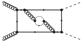
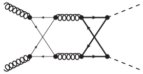
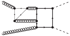
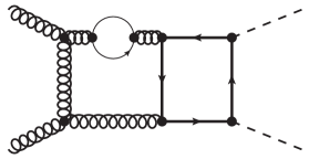
Figure 1: Sample Feynman diagrams. Curly lines denote gluons, dashed ones Higgs bosons, while thin (thick) lines are massless (top) quarks.

In this letter we consider $t=0$ and $m_{H}=0$, i.e. the leading term in an expansion around $t\to 0$ and $m_{H}\to 0$. This constitutes a crude approximation, however, in a large part of the phase space it contributes a major part of the corrections. For example, choosing $t=0$ and $m_{H}=0$ at two loops (NLO), at a transverse momentum of $p_{T}=100$ GeV the form factor $F_{\rm box1}$ deviates from its exact value by at most 30%, depending on the value of $\sqrt{s}$ considered. This means that more than two thirds of the form factor value are covered by the $t=0$, $m_{H}=0$ approximation. Furthermore, we concentrate on the one-particle irreducible contributions. We note that $F_{\rm box2}$ vanishes for $t=0$. More details are given below in Section 3.

We present here results for the light-fermionic (“$n_{l}$”) terms and show that this approach can be used to obtain the three-loop virtual corrections to $gg\to HH$. The remaining contributions contain many more integral topologies and more complicated integrals, which have to be integration-by-parts (IBP) reduced to master integrals.

In the next section we outline the techniques used for the calculations and discuss the results in Section 3. In Section 4 we conclude and provide an outlook for the computation of the full corrections.

2 Technical Details

The basic philosophy of our calculation has already been outlined in Ref. [6], where the two-loop amplitude for $gg\to HH$ has been considered in the small-$t$ and high-energy limit and it has been shown that the combination of both expansions covers the whole phase-space. The starting point for both expansions is the amplitude expressed in terms of the same master integrals which are obtained from a reduction problem which involves the dimensional variables $s$, $t$ and $m_{t}$. Using currently available tools such a reduction is not possible at three loops. To avoid such an IBP reduction, one can try to expand the unreduced amplitude in the respective limit. The high-energy expansion is obtained via a complicated asymptotic expansion which involves a large number of different regions. On the other hand, the limit $t\to 0$ leads to a simple Taylor expansion which can be easily realized at the level of the integrands. Furthermore, the expansion around forward-scattering kinematics covers a large part of the physically relevant phase space [5].

Our computation begins by generating the amplitude with qgraf [28], and then using tapir [29] and exp [30, 31] to map the diagrams onto integral topologies and convert the output to FORM [32] notation. The diagrams are then computed with the in-house “calc” setup, to produce an amplitude in terms of scalar Feynman integrals. These tools work together to provide a high degree of automation. We perform the calculation for general QCD gauge parameter which drops out once the amplitude is expressed in terms of master integrals. This is a welcome check for our calculation.

The scalar integrals can be Taylor expanded in $m_{H}$ at this point, as done at two loops in Refs. [33, 34, 6], however at three loops in this letter we keep only the leading term in this expansion, i.e., set $m_{H}=0$.

The next step is to expand the amplitude around the forward kinematics ($t\to 0$) at the integrand level. This is implemented in FORM by introducing $q_{\delta}=q_{1}+q_{3}$ in the propagators and expanding in $q_{\delta}$ to the required order. Note that $q_{\delta}^{2}=t$. After treating the tensor integrals, where $q_{\delta}$ appears contracted with a loop momentum, we need to perform a partial-fraction decomposition to eliminate linearly dependent propagators. The partial fractioning rules are produced automatically by tapir when run with the forward kinematics ($q_{3}=-q_{1}$) specified. Note that although for the present publication we compute the “$t=0$ contribution”, we must properly expand in $q_{\delta}$ to produce the amplitude to order $t^{0}$ due to inverse powers of $t$ appearing in the projectors. These inverse powers ultimately cancel in the final result. This procedure yields amplitudes for $F_{\rm box1}$ and $F_{\rm box2}$ in terms of scalar Feynman integrals which belong to topologies which depend only on $s$ and $m_{t}$ (and not on $t$).

At this point the amplitudes are written in terms of 60 integral topologies, however these are not all independent; they can be reduced to a smaller set by making use of loop-momentum shifts and identification of common sub-sectors. In one approach we find these rules with the help of LiteRed [36], which identifies a minimal set of 28 topologies. In a second approach we use Feynson [37] to generate these maps and end up with 53 topologies. The difference in the number of topologies is due to LiteRed mapping topology sub-sectors, while we used Feynson only at the top level. When considering the full amplitude, i.e., not just the light-fermionic corrections, only the Feynson approach is feasible for performance reasons. It is also possible to use Feynson to find sub-sector mappings, which we will also use when considering the full amplitude (which is written initially in terms of 522 integral topologies).

The amplitude is now ready for a reduction to master integrals using Kira [38] and FireFly [39, 40]. The most complicated integral topology took about a week on a 16-core node, using around 500GB of memory. After minimizing the final set of master integrals across the topologies with Kira, we are left with 177 master integrals to compute. Comparing results obtained via the LiteRed and Feynson topology-mapping approaches reveals one additional relation within this set which is missed by Kira, however, we compute the set of 177 master integrals which was first identified.

To compute the master integrals, we first establish a system of differential equations w.r.t. $x=s/m_{t}^{2}$. Boundary conditions are provided in the large-$m_{t}$ ($x\to 0$) limit: we prepare the three-loop integrals in the forward kinematics, and pass them to exp which automates the asymptotic expansion in the limit that $m_{t}^{2}\gg s$. This leads to three-loop vacuum integrals, as well as products of one- and two-loop vacuum integrals with two- and one-loop massless $s$-channel $2\to 1$ integrals, respectively. This expansion leads to tensor vacuum integrals, which our “calc” setup can compute up to rank 10. We compute the first two expansion terms in $s/m_{t}^{2}$ for each of the 177 master integrals. To fix the boundary constants for the differential equations we only need about half of the computed coefficients; the rest serve as consistency checks.

The differential equations are then used to produce 100 expansion terms for the forward-kinematics master integrals in the large-$m_{t}$ limit which we use to compute $F_{\rm box1}$. Since these results are analytic in the large-$m_{t}$ limit we can compare with the results obtained in Ref. [13] in the limit $t=0$, and find agreement.

The final step is to use the “expand and match” approach [17, 18] to obtain “semi-analytic” results which cover the whole $s$ range. Note that this approach properly takes into account the threshold effects at the point $s=4m_{t}^{2}$. “Semi analytic” means that our final results consist of expansions around a set of $x$ values, where the expansion coefficients are available only numerically. Starting from the (analytic) expansion around $x=0$, each expansion provides numeric boundary conditions to fix the coefficients of the subsequent expansion. Each expansion is only ever evaluated within its radius of convergence.

3 Three-loop light-fermionic contributions to $F_{\rm box1}$

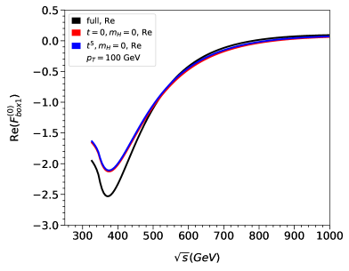
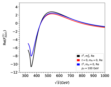
Figure 2: The real part of $F_{\rm box1}$ at one and two loops, for $p_{T}=100$ GeV. The $t=0$, $m_{H}=0$ approximation is shown in red, and the $t^{5},m_{H}=0$ approximation in blue. At one loop we compare with the exact result with full $m_{H}$ and $t$ dependence, in black. At two loops, in lieu of an exact result, we compare with the $t^{5},m_{H}^{4}$ approximation, in black.

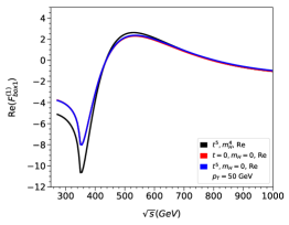
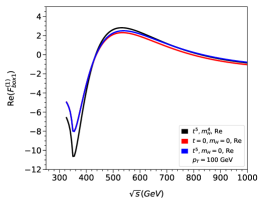
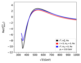
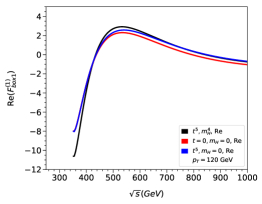
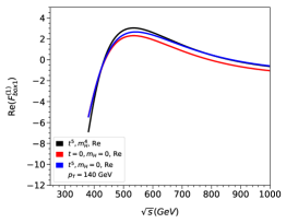
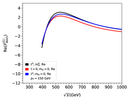
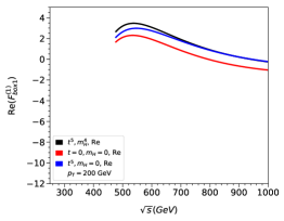
Figure 3: Two-loop results for various values of $p_{T}$. The meaning of the curves is described in the caption to Fig. 2. Note that the red curves are independent of $p_{T}$ and thus they are identical in all panels.

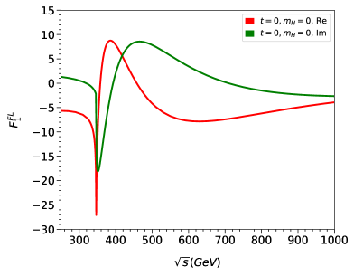
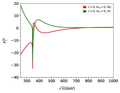
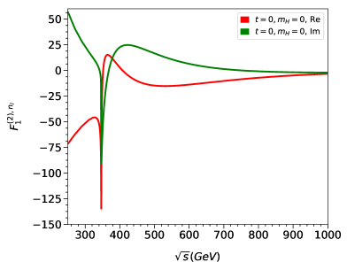
Figure 4: Real (red) and imaginary (green) parts of $F_{\rm box1}^{FL}$, $F_{\rm box1}^{AL}$ and $F_{\rm box1}^{(2),n_{l}}$ as a function of $\sqrt{s}$.

In this section we present the light-fermionic three-loop corrections to the form factor $F_{\rm box1}$ for Higgs boson pair production. We note again that in our $t=0,m_{H}=0$ approximation, $F_{\rm box2}$ vanishes; we observe this after IBP reduction and writing the result in terms of the minimal set of master integrals.

We obtain the renormalized form factors after the renormalization of the parameters $\alpha_{s}$ and $m_{t}$ and the wave functions of the gluons in the initial state. We then express our results in terms of $\alpha_{s}^{(5)}$ and treat the remaining infrared divergences following Ref. [41]. This leads to finite results for $F_{\rm box1}$. In the following we present numerical results. For the top quark and Higgs boson masses, we use the values $m_{t}=173.21$ GeV and $m_{H}=125.1$ GeV.

Let us first discuss the one- and two-loop results. In Fig. 2 we show the real part of $F_{\rm box1}$ for $p_{T}=100$ GeV. In red, we show the approximation that we use at three loops, i.e., $t=0$ and $m_{H}=0$. In black, we show curves with the full dependence on $t$ and $m_{H}$. At one loop this is the fully exact result, but at two loops this is an expansion to order $t^{5}$ and $m_{H}^{4}$; we have shown in Ref. [6] that this provides an extremely good approximation of the (unknown) fully exact result. We observe that the $t=0$, $m_{H}=0$ curves approximate the “exact” results with an accuracy of about 30% in the region below about $\sqrt{s}=500$ GeV. For higher energies the approximation works better.

In Fig. 2 we also show blue curves which include expansion terms up to $t^{5}$, but still only the leading term in the $m_{H}$ expansion. These curves lie very close to the red $t=0$, $m_{H}=0$ curves, which show that for $p_{T}\approx 100$ GeV it is more important to incorporate additional terms in the $m_{H}$ expansion than in the $t$ expansion. For higher values of $p_{T}$ we expect that higher $t$ expansion terms become more important. This can be seen in Fig. 3 where results of the two-loop form factor are shown for various values of $p_{T}$. The panels also show that a large portion of the cross section is covered by the $t=0$ approximation, even for $p_{T}=200$ GeV where, for lower values of $\sqrt{s}$, about 50% are captured by the red curve.

In Fig. 4 we show the new results obtained in this letter. The plots show both the real (in red) and imaginary (in green) parts of the light-fermionic part of $F_{\rm box1}$, both separated into the $C_{F}$ and $C_{A}$ colour factor contributions, and their combination. We observe a strong variation of the form factor around the top quark pair threshold region. This behaviour is not caused by a loss of precision of our semi-analytic expansions around this threshold; indeed $F_{\rm box1}$ is finite in the limit $s\to 4m_{t}^{2}$, however whereas at two loops we observe leading logarithmic contributions which go like $v\log{v}$, where $v=\sqrt{1-4m_{t}^{2}/s}$, at three loops we find an additional power of $\log{v}$ which is responsible for the large variation around this point.

The numerical value of the light-fermionic contribution to $F_{\rm box1}$ at three-loops exceeds the size of the two-loop form factor by almost an order of magnitude. Although this is compensated by the additional factor of $\alpha_{s}/\pi$, this hints at sizeable three-loop corrections. However, for a final conclusion, the remaining diagrams need to be computed. The full computation will also allow a study of the top quark mass scheme dependence. These issues will be addressed in a future publication.

4 Conclusions

The computation of three-loop corrections to $2\to 2$ scattering processes with massive internal particles is a technically challenging task. Currently-available techniques are most likely not sufficient to obtain analytic or numerical results without applying any approximation. In this letter we apply the ideas of Refs. [5, 16, 6] to $gg\to HH$ and show that three-loop corrections can be obtained. We concentrate on the light-fermionic three-loop contributions which is a well-defined and gauge-invariant subset. The obtained results are valid for $t=0$ and $m_{H}=0$ which approximates the full result to 30% or better for $p_{T}\approx 100$ GeV.

The approach outlined in this letter can also be used to compute the remaining colour factor contributions, which are needed to study the overall impact of the three-loop virtual corrections and also the top quark mass renormalization scheme dependence.

In addition to the remaining colour factors, we ultimately aim to compute the $t^{1}\,m_{H}^{2}$ approximation which would address the 30% error discussed in Section 3, improve the approximation for higher values of $p_{T}$, and provide a non-zero value for $F_{\rm box2}$. To compute these terms will require significantly more CPU time and, most likely, improvements to IBP reduction software in order to efficiently reduce the large numbers of integrals produced by the expansions.

References

- [1] E. W. N. Glover and J. J. van der Bij, Nucl. Phys. B 309 (1988), 282-294
- [2] S. Borowka, N. Greiner, G. Heinrich, S. P. Jones, M. Kerner, J. Schlenk, U. Schubert and T. Zirke, Phys. Rev. Lett. 117 (2016) no.1, 012001 [erratum: Phys. Rev. Lett. 117 (2016) no.7, 079901] [arXiv:1604.06447 [hep-ph]].
- [3] S. Borowka, N. Greiner, G. Heinrich, S. P. Jones, M. Kerner, J. Schlenk and T. Zirke, JHEP 10 (2016), 107 [arXiv:1608.04798 [hep-ph]].
- [4] J. Baglio, F. Campanario, S. Glaus, M. Mühlleitner, M. Spira and J. Streicher, Eur. Phys. J. C 79 (2019) no.6, 459 [arXiv:1811.05692 [hep-ph]].
- [5] L. Bellafronte, G. Degrassi, P. P. Giardino, R. Gröber and M. Vitti, JHEP 07 (2022), 069 doi:10.1007/JHEP07(2022)069 [arXiv:2202.12157 [hep-ph]].
- [6] J. Davies, G. Mishima, K. Schönwald and M. Steinhauser, JHEP 06 (2023), 063 [arXiv:2302.01356 [hep-ph]].
- [7] D. de Florian and J. Mazzitelli, Phys. Rev. Lett. 111 (2013), 201801 [arXiv:1309.6594 [hep-ph]].
- [8] D. de Florian and J. Mazzitelli, Phys. Lett. B 724 (2013), 306-309 [arXiv:1305.5206 [hep-ph]].
- [9] J. Grigo, K. Melnikov and M. Steinhauser, Nucl. Phys. B 888 (2014), 17-29 [arXiv:1408.2422 [hep-ph]].
- [10] L. B. Chen, H. T. Li, H. S. Shao and J. Wang, Phys. Lett. B 803 (2020), 135292 [arXiv:1909.06808 [hep-ph]].
- [11] L. B. Chen, H. T. Li, H. S. Shao and J. Wang, JHEP 03 (2020), 072 [arXiv:1912.13001 [hep-ph]].
- [12] J. Grigo, J. Hoff and M. Steinhauser, Nucl. Phys. B 900 (2015), 412-430 [arXiv:1508.00909 [hep-ph]].
- [13] J. Davies and M. Steinhauser, JHEP 10 (2019), 166 [arXiv:1909.01361 [hep-ph]].
- [14] J. Davies, F. Herren, G. Mishima and M. Steinhauser, JHEP 01 (2022), 049 [arXiv:2110.03697 [hep-ph]].
- [15] J. Baglio, F. Campanario, S. Glaus, M. Mühlleitner, J. Ronca and M. Spira, Phys. Rev. D 103 (2021) no.5, 056002 [arXiv:2008.11626 [hep-ph]].
- [16] G. Degrassi, R. Gröber, M. Vitti and X. Zhao, JHEP 08 (2022), 009 doi:10.1007/JHEP08(2022)009 [arXiv:2205.02769 [hep-ph]].
- [17] M. Fael, F. Lange, K. Schönwald and M. Steinhauser, SciPost Phys. Proc. 7 (2022), 041 [arXiv:2110.03699 [hep-ph]].
- [18] M. Fael, F. Lange, K. Schönwald and M. Steinhauser, Phys. Rev. D 106 (2022) no.3, 034029 [arXiv:2207.00027 [hep-ph]].
- [19] G. Degrassi, P. P. Giardino and R. Gröber, Eur. Phys. J. C 76 (2016) no.7, 411 [arXiv:1603.00385 [hep-ph]].
- [20] T. Plehn, M. Spira and P. M. Zerwas, Nucl. Phys. B 479 (1996), 46-64 [erratum: Nucl. Phys. B 531 (1998), 655-655] [arXiv:hep-ph/9603205 [hep-ph]].
- [21] R. Harlander and P. Kant, JHEP 12 (2005), 015 [arXiv:hep-ph/0509189 [hep-ph]].
- [22] C. Anastasiou, S. Beerli, S. Bucherer, A. Daleo and Z. Kunszt, JHEP 01 (2007), 082 [arXiv:hep-ph/0611236 [hep-ph]].
- [23] U. Aglietti, R. Bonciani, G. Degrassi and A. Vicini, JHEP 01 (2007), 021 [arXiv:hep-ph/0611266 [hep-ph]].
- [24] J. Davies, R. Gröber, A. Maier, T. Rauh and M. Steinhauser, Phys. Rev. D 100 (2019) no.3, 034017 [erratum: Phys. Rev. D 102 (2020) no.5, 059901] [arXiv:1906.00982 [hep-ph]].
- [25] J. Davies, R. Gröber, A. Maier, T. Rauh and M. Steinhauser, PoS RADCOR2019 (2019), 079 [arXiv:1912.04097 [hep-ph]].
- [26] R. V. Harlander, M. Prausa and J. Usovitsch, JHEP 10 (2019), 148 [erratum: JHEP 08 (2020), 101] [arXiv:1907.06957 [hep-ph]].
- [27] M. L. Czakon and M. Niggetiedt, JHEP 05 (2020), 149 doi:10.1007/JHEP05(2020)149 [arXiv:2001.03008 [hep-ph]].
-
[28]
P. Nogueira,
J. Comput. Phys. 105 (1993), 279-289;
http://cfif.ist.utl.pt/~paulo/qgraf.html. - [29] M. Gerlach, F. Herren and M. Lang, Comput. Phys. Commun. 282 (2023), 108544 [arXiv:2201.05618 [hep-ph]].
- [30] R. Harlander, T. Seidensticker and M. Steinhauser, Phys. Lett. B 426 (1998) 125 [hep-ph/9712228].
- [31] T. Seidensticker, hep-ph/9905298.
- [32] B. Ruijl, T. Ueda and J. Vermaseren, [arXiv:1707.06453 [hep-ph]].
- [33] J. Davies, G. Mishima, M. Steinhauser and D. Wellmann, JHEP 03 (2018), 048 [arXiv:1801.09696 [hep-ph]].
- [34] J. Davies, G. Mishima, M. Steinhauser and D. Wellmann, JHEP 01 (2019), 176 [arXiv:1811.05489 [hep-ph]].
- [35] F. Herren, “Precision Calculations for Higgs Boson Physics at the LHC - Four-Loop Corrections to Gluon-Fusion Processes and Higgs Boson Pair-Production at NNLO,” PhD thesis, 2020, KIT.
- [36] R. N. Lee, J. Phys. Conf. Ser. 523 (2014), 012059 [arXiv:1310.1145 [hep-ph]].
-
[37]
V. Magerya,
“Semi- and Fully-Inclusive Phase-Space Integrals at Four Loops,”
Dissertation, University of Hamburg, 2022.
https://github.com/magv/feynson. - [38] J. Klappert, F. Lange, P. Maierhöfer and J. Usovitsch, Comput. Phys. Commun. 266 (2021), 108024 [arXiv:2008.06494 [hep-ph]].
- [39] J. Klappert, S. Y. Klein and F. Lange, Comput. Phys. Commun. 264 (2021), 107968 [arXiv:2004.01463 [cs.MS]].
- [40] J. Klappert and F. Lange, Comput. Phys. Commun. 247 (2020), 106951 [arXiv:1904.00009 [cs.SC]].
- [41] S. Catani, Phys. Lett. B 427 (1998), 161-171 [arXiv:hep-ph/9802439 [hep-ph]].