CHEX-MATE: CLUster Multi-Probes in Three Dimensions (CLUMP-3D)

Galaxy clusters are the products of structure formation through myriad physical processes that affect their growth and evolution throughout cosmic history. As a result, the matter distribution within galaxy clusters, or their shape, is influenced by cosmology and astrophysical processes, in particular the accretion of new material due to gravity. We introduce an analysis method to investigate the three-dimensional triaxial shapes of galaxy clusters from the Cluster HEritage project with XMM-Newton – Mass Assembly and Thermodynamics at the Endpoint of structure formation (CHEX-MATE). In this work, the first paper of a CHEX-MATE triaxial analysis series, we focus on utilizing X-ray data from XMM-Newton and Sunyaev-Zel’dovich (SZ) effect maps from Planck and Atacama Cosmology Telescope (ACT) to obtain a three dimensional triaxial description of the intracluster medium (ICM) gas. We present the forward modeling formalism of our technique, which projects a triaxial ellipsoidal model for the gas density and pressure to compare directly with the observed two dimensional distributions in X-rays and the SZ effect. A Markov chain Monte Carlo is used to estimate the posterior distributions of the model parameters. Using mock X-ray and SZ observations of a smooth model, we demonstrate that the method can reliably recover the true parameter values. In addition, we apply the analysis to reconstruct the gas shape from the observed data of one CHEX-MATE galaxy cluster, PSZ2 G313.33+61.13 (Abell 1689), to illustrate the technique. The inferred parameters are in agreement with previous analyses for that cluster, and our results indicate that the geometrical properties, including the axial ratios of the ICM distribution, are constrained to within a few percent. With much better precision than previous studies, we thus further establish that Abell 1689 is significantly elongated along the line of sight, resulting in its exceptional gravitational lensing properties.

1 Introduction

Galaxy clusters are useful probes of structure formation, astrophysical processes such as shocks and feedback from active galactic nuclei, and cosmology (Davis et al., 1985; Voit, 2005; Allen et al., 2011; Kravtsov & Borgani, 2012; Markevitch & Vikhlinin, 2007; McNamara & Nulsen, 2007). For instance, they are fundamental to the science goals of numerous ongoing and upcoming large survey projects such as eROSITA (Predehl et al., 2021), Euclid (Euclid Collaboration et al., 2019), and Rubin Observatory (Ivezić et al., 2019). In order to maximize the scientific reach of such programs, particularly with regard to cosmological parameter constraints, it is crucial to accurately characterize the ensemble average physical properties of galaxy clusters along with the intrinsic scatter relative to these averages (e.g., Lima & Hu, 2005; Zhan & Tyson, 2018; Euclid Collaboration et al., 2019). One such example are the scaling relations used to connect global galaxy cluster observables to underlying halo mass (Rozo & Rykoff, 2014; Mantz et al., 2016; Pratt et al., 2019). While these scaling relations are generally sensitive to a range of astrophysical processes (e.g., Ansarifard et al., 2020), some observables, including the gravitational weak lensing measurements often used to determine absolute mass, have deviations from average relations that are dominated by projection effects related to asphericity and orientation (Meneghetti et al., 2010; Becker & Kravtsov, 2011).

CHEX-MATE (CHEX-MATE Collaboration et al., 2021) is an effort to provide a more accurate understanding of the population of galaxy clusters at low-$z$ and high mass, particularly in the context of cosmology and mass calibration, including the shape of their matter distributions and the effects of the baryonic physics on their global properties. The project is based on a 3 Msec XMM-Newton program to observe 118 galaxy clusters, containing two equal-sized sub-samples selected from the Planck all-sky SZ effect survey. The CHEX-MATE Tier-1 and Tier-2 samples each include 61 galaxy clusters with four overlapping clusters and represent a volume-limited ($0.05<z\leq 0.2$) sample in the local universe and mass-limited ($M_{500}\geq 7.25\times 10^{14}\leavevmode\nobreak\ \textrm{M}_{\odot}$) sample of the most massive objects in the universe, respectively. The X-ray observing program has recently been completed, and initial results from the analyses of these data along with publicly available SZ data have already been published (Campitiello et al., 2022; Oppizzi et al., 2022; Bartalucci et al., 2023).

We utilize triaxial modeling techniques (e.g., Limousin et al., 2013) to investigate the three-dimensional mass distribution within the CHEX-MATE galaxy clusters to infer their intrinsic properties. This approach is motivated by two reasons: (1) Three-dimensional triaxial shapes provide a better approximation of galaxy clusters than spherical models, and the parameters, such as mass, obtained from such an analysis have lower levels of bias and intrinsic scatter (Becker & Kravtsov, 2011; Khatri & Gaspari, 2016); (2) A correlation between the triaxial shape of the dark matter (DM) halo and its formation history has been established in simulations (e.g., Ho et al., 2006; Lau et al., 2021; Stapelberg et al., 2022), suggesting that triaxial shape measurements can provide a powerful probe of cosmology independent of other techniques currently in use. For instance, some lensing-based shape measurements have found good agreement with $\Lambda$CDM predictions (Oguri et al., 2010; Chiu et al., 2018), while a recent multi-probe triaxial analysis suggests a $\simeq 2\sigma$ discrepancy between the observed and predicted minor to major axial ratio distributions (Sereno et al., 2018). This discrepancy could indicate that clusters formed more recently than predicted. Alternatively, elevated merger rates (Despali et al., 2017), a reduced influence of baryons on the dark matter (Suto et al., 2017) or enhanced feedback (Kazantzidis et al., 2004) could also explain the observed cluster shapes. CHEX-MATE offers a uniform selection of galaxy clusters with consistent measurements of ICM density and temperature. This clean, well-characterized selection with a large sample size ($\sim\!80$ clusters excluding major mergers; Campitiello et al. 2022) will enable a robust cosmological measurement of the triaxial shape distribution.

For our analysis, we adopted the CLUster Multi-Probes in Three Dimensions (CLUMP-3D; Sereno et al., 2017, 2018; Chiu et al., 2018; Sayers et al., 2021) project and implemented significant updates to the modeling package. CLUMP-3D incorporates multiwavelength data from X-ray (surface brightness and spectroscopic temperature), mm-wave (SZ surface brightness), and optical (gravitational lensing) observations, which are the projected observables. Then, it assumes triaxial distributions of the ICM gas and matter density profiles. Taking advantage of the different dependencies of the X-ray and SZ signals on the gas density and temperature, they probe the line-of-sight extent of the ICM, and gravitational lensing data probes the projected matter distribution. In particular, the X-ray emission observed from the ICM is proportional to the line-of-sight integral of the squared electron density ($n_{e}$) multiplied by the X-ray cooling function, $\Lambda$, represented as $S_{X}\propto\int n^{2}_{e}\Lambda dl$. Meanwhile, the detected SZ signal is proportional to the line-of-sight integral of the product of electron density and temperature ($T_{e}$), denoted as $B_{\textrm{SZ}}\propto\int n_{e}T_{e}dl$. Given that the ICM temperature ($T_{X}$) can be spectroscopically measured using X-ray observations, the line-of-sight elongation ($\triangle l$) can subsequently be determined through the combination of these three measurements as $\triangle l\sim(B^{2}_{\textrm{SZ}}\Lambda)/(S_{X}T^{2}_{X})$. Assuming co-alignement of the triaxial axes of the ICM and dark matter distributions, while still allowing for different axial ratios for the two quantities, our multi-probe analysis can thus constrain the three-dimensional shapes of galaxy clusters. CLUMP-3D was introduced in Sereno et al. (2017), where the authors inferred the triaxial matter and gas distribution of the galaxy cluster MACS J1206.2$-$0847. The technique built upon similar methods developed to constrain cluster morphology (e.g., Sereno & Umetsu, 2011; Sereno et al., 2012). Then, it was applied to measure the shapes of the Cluster Lensing And Supernova survey with Hubble (CLASH; Postman et al., 2012) clusters, to probe the ensemble-average three-dimensional geometry (Sereno et al., 2018; Chiu et al., 2018) as well as the radial profile of the non-thermal pressure fraction (Sayers et al., 2021). These results demonstrated the potential of the three-dimensional triaxial shape measurement technique, but they were relatively imprecise due to the sample size, data quality, and systematics related to cluster selection. Thus, the much larger CHEX-MATE galaxy cluster sample, with a well understood selection function and more uniform and higher quality X-ray data, will provide improved statistics and more robust constraints on the shape measurements.

In this paper, we demonstrate several improvements to the original CLUMP-3D formalism while modeling the ICM distributions observed by XMM-Newton, Planck, and ground-based SZ data from ACT. As detailed below, we have implemented a fully two-dimensional analysis of the X-ray temperature (Lovisari et al., 2023) and SZ data, whereas the original CLUMP-3D only treated the X-ray surface brightness (SB) in two dimensions while using one-dimensional azimuthally-averaged profiles of both the X-ray spectroscopic temperatures and the SZ effect data. In addition, we now model the ICM gas density and pressure instead of its density and temperature. This allows us to fit the data with fewer parameters, thus accelerating the model fitting process. Additionally, we fully rewrote the code in Python to facilitate future public release of the package. In Sec. 2, we summarize the triaxial analysis formalism and describe the model fitting method. In Sec. 3, we introduce the X-ray and SZ data from our program and apply the technique to a CHEX-MATE galaxy cluster. In a subsequent paper, we will include gravitational lensing constraints in a manner that also builds upon, and improves, the existing CLUMP-3D technique. With these X-ray, SZ effect, and gravitational lensing data, we will be able to model the triaxial distributions of both the ICM and the dark matter. Throughout this study, we adopt a $\Lambda$CDM cosmology characterized by $H_{0}=70\leavevmode\nobreak\ \textrm{km}\leavevmode\nobreak\ \textrm{s}^{-1}\leavevmode\nobreak\ \textrm{Mpc}^{-1}$, $\Omega_{\textrm{m}}=0.3$, and $\Omega_{\Lambda}=0.7$. $E(z)$ represents the ratio of the Hubble constant at redshift $z$ to its present value, $H_{0}$, and $h_{70}=H_{0}/(100\leavevmode\nobreak\ \textrm{s}^{-1}\leavevmode\nobreak\ \textrm{Mpc}^{-1})/0.7$.

2 Triaxial Analysis: Formalism and the Model fit

While the mathematical description of a triaxial geometry for astronomical objects and their physical profiles has been introduced in previous studies (e.g., Stark, 1977; Binggeli, 1980; Binney, 1985; Oguri et al., 2003; De Filippis et al., 2005; Corless & King, 2007; Sereno et al., 2010, 2012, 2018), these works lack consistency in their notation. To prevent confusion, we present our mathematical formalism for triaxial modeling in this section. We then describe our model fitting procedure and the implementation of the fitting algorithm in our software package.

As this paper focuses on the analysis method to study ICM distributions, we do not include the gravitational lensing data in our fits. Future works in this series will expand our formalism to include total mass density profiles constrained by gravitational lensing measurements. For instance, in the case of a Navarro–Frenk–White (NFW; Navarro et al., 1997) profile the gravitational lensing analysis requires two additional parameters–total mass ($M_{200}$) and concentration ($c_{200}$)–assuming that the gas and matter distributions are co-aligned along the ellipsoidal axes. This assumption is well supported by a 2D weak-lensing and X-ray analysis of 20 high-mass galaxy clusters (Umetsu et al., 2018), as well as by cosmological hydrodynamical simulations (Okabe et al., 2018).

2.1 Geometry and Projection

To connect the intrinsic cluster geometry to the projected properties observed in the plane of the sky, we assume a triaxial ellipsoidal model for the gas distribution, where the thermodynamic profiles of the ICM are represented as a function of $\zeta$, the ellipsoidal radius. In the intrinsic coordinate system of the ellipsoid $(x_{1},x_{2},x_{3})$, it is defined as:

$$\zeta^{2}=\frac{x^{2}_{1}}{q^{2}_{1}}+\frac{x^{2}_{2}}{q^{2}_{2}}+x^{2}_{3},$$ (1)

where $q_{1}$ and $q_{2}$ are minor-to-major and intermediate-to-major axial ratios, respectively ($0<q_{1}\leq q_{2}\leq 1$). Given a semi-major axis of the ellipsoid $l_{s}$, the volume of the ellipsoid is $(4\pi/3){l^{3}_{s}}q_{1}q_{2}$. The ellipsoid becomes a prolate shape if $q_{1}=q_{2}\leq 1$ and an oblate shape if $q_{1}\leq q_{2}=1$.

Figure 1 illustrates the geometry of the ellipsoid and the involved coordinate systems. It is essential to note that the axes defining the ICM model may not align with the observer’s frame. To relate the ellipsoid’s intrinsic coordinate system ($x^{\text{\tiny int}}_{1}$, $x^{\text{\tiny int}}_{2}$, $x^{\text{\tiny int}}_{3}$) to the observer’s coordinate frame ($x^{\text{\tiny obs}}_{1}$, $x^{\text{\tiny obs}}_{2}$, $x^{\text{\tiny obs}}_{3}$), we employ three Euler angles. These angles describe the relationship between the two coordinate systems: (1) the angle between $x^{\text{\tiny int}}_{3}$, aligned with the major axis of the ellipsoid, and $x^{\text{\tiny obs}}_{3}$, which lies along the observer’s line-of-sight ($\theta$), (2) the angle between $x^{\text{\tiny int}}_{1}$ and the line of nodes ($\varphi$), and (3) the angle between $x^{\text{\tiny obs}}_{1}$ and the line of nodes ($\psi$). The line of nodes is the intersection of the $x^{\text{\tiny int}}_{1}$-$x^{\text{\tiny int}}_{2}$ plane and the $x^{\text{\tiny obs}}_{1}$-$x^{\text{\tiny obs}}_{2}$ plane, and it is aligned with the vector $x^{\text{\tiny int}}_{3}\times x^{\text{\tiny obs}}_{3}$.

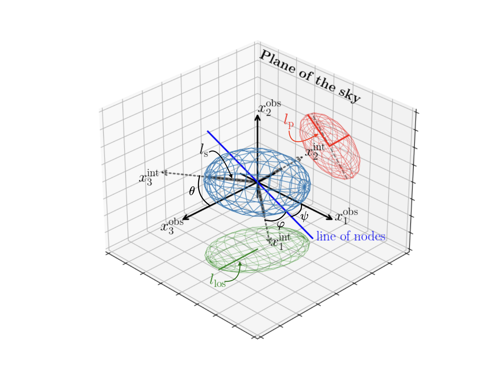
Figure 1: This figure depicts the triaxial ellipsoid model and the coordinate systems used in the triaxial analysis. The intrinsic coordinate system of the ellipsoid is denoted by dotted grey arrows ($x^{\text{\tiny int}}_{1}$, $x^{\text{\tiny int}}_{2}$, and $x^{\text{\tiny int}}_{3}$), where $x^{\text{\tiny int}}_{3}$ represents the major axis. The black arrows ($x^{\text{\tiny obs}}_{1}$, $x^{\text{\tiny obs}}_{2}$, and $x^{\text{\tiny obs}}_{3}$) correspond to the observer’s coordinate system, where $x^{\text{\tiny obs}}_{3}$ is aligned with the observer’s line-of-sight. In other words, an observer views the ellipsoid in the $-x^{\text{\tiny obs}}_{3}$ direction. The three Euler angles ($\theta$, $\varphi$, $\psi$) characterize the intrinsic coordinate system of the ellipsoid in relation to the observer’s coordinate system. The blue line represents the line of nodes, which is the intersection of the $x^{\text{\tiny int}}_{1}$-$x^{\text{\tiny int}}_{2}$ plane and the $x^{\text{\tiny obs}}_{1}$-$x^{\text{\tiny obs}}_{2}$ plane, and it is aligned with the vector $x^{\text{\tiny int}}_{3}\times x^{\text{\tiny obs}}_{3}$. The red ellipse denotes the projection of the ellipsoid on the sky plane, with $l_{\textrm{p}}$ representing its semi-major axis. The black dashed line on the ellipse shows the projected major axis of the ellipsoid on the sky plane. The green ellipse is the projection of the ellipsoid onto the plane that is perpendicular to the sky plane, and $l_{\text{\tiny los}}$ is the half size of the ellipse along the observer line-of-sight. See also Figs. 2. and 3. in Sereno et al. (2012).

We can derive the geometric properties of the projected ellipse from the intrinsic parameters of the ellipsoid when it is projected onto the plane from any direction. These properties encompass the semi-major axis of the projected ellipse $l_{\textrm{p}}$, its ellipticity $\epsilon$, the orientation of the ellipse in the plane of the sky $\theta_{\epsilon}$, and the elongation parameter $e_{\parallel}$. The projected profiles are expressed as a function of $\xi$, the elliptical radius of the ellipse in the plane of the sky.

The ellipticity of the projected ellipse ($\epsilon$) is

$$\epsilon=1-q_{\textrm{p}},$$ (2)

where $q_{\textrm{p}}$ is the minor-to-major axial ratio of the observed projected isophote ($q_{\textrm{p}}\leq 1$), which is the inverse of $e_{\textrm{p}}$ used in Sereno et al. (2012), and

$$q_{\textrm{p}}=\sqrt{\frac{j+l-\sqrt{(j-l)^{2}+4k^{2}}}{j+l+\sqrt{(j-l)^{2}+4k^{2}}}},$$ (3)

where

$$j = \frac{1}{2}\left[\left(\frac{1}{q^{2}_{1}}+\frac{1}{q^{2}_{2}}\right)-\frac{\sin^{2}\theta\cos^{2}\psi\left(q^{2}_{1}+q^{2}_{2}-2\right)}{q^{2}_{1}q^{2}_{2}}+\left(\frac{1}{q^{2}_{1}}-\frac{1}{q^{2}_{2}}\right)\left\{\cos 2\varphi\left(\cos^{2}\theta\cos^{2}\psi-\sin^{2}\psi\right)-\cos\theta\sin 2\varphi\sin 2\psi\right\}\right],$$

$$k = \frac{1}{4q^{2}_{1}q^{2}_{2}}\left[2\cos\theta\left(q^{2}_{1}-q^{2}_{2}\right)\cos 2\psi\sin 2\varphi+\left\{\sin^{2}\theta\left(q^{2}_{1}+q^{2}_{2}-2\right)+\left(1+\cos^{2}\theta\right)\left(q^{2}_{1}-q^{2}_{2}\right)\cos 2\varphi\right\}\sin 2\psi\right],$$ (4)

$$l = \frac{1}{2}\left[\left(\frac{1}{q^{2}_{1}}+\frac{1}{q^{2}_{2}}\right)-\frac{\sin^{2}\theta\sin^{2}\psi\left(q^{2}_{1}+q^{2}_{2}-2\right)}{q^{2}_{1}q^{2}_{2}}+\left(\frac{1}{q^{2}_{1}}-\frac{1}{q^{2}_{2}}\right)\left\{\cos 2\varphi\left(\cos^{2}\theta\sin^{2}\psi-\cos^{2}\psi\right)+\cos\theta\sin 2\varphi\sin 2\psi\right\}\right].$$

It is worth noting that the expressions of $j$, $k$, and $l$ in Stark (1977) and Binggeli (1980) differ from those presented above, as they assumed $\psi=0$, using only two angles to align the major ellipsoidal axis with the observer’s line-of-sight. However, a coordinate transformation requiring $\psi$ is necessary to align the remaining axes.

The orientation angle in the plane of the sky of the projected ellipse is

$$\theta_{\epsilon}=\tan^{-1}\left(\frac{l-j+\sqrt{(j-l)^{2}+4k^{2}}}{2k}\right),$$ (5)

and the elongation parameter of the ellipsoid is

$$e_{\parallel}\equiv\frac{l_{\textrm{los}}}{l_{\textrm{p}}}=\sqrt{\frac{q_{\textrm{p}}}{q_{1}q_{2}}}f^{-3/4},$$ (6)

where

$$f=\sin^{2}\theta\left[\left(\frac{\sin\varphi}{q_{1}}\right)^{2}+\left(\frac{\cos\varphi}{q_{2}}\right)^{2}\right]+\cos^{2}\theta.$$ (7)

The elongation parameter, $e_{\parallel}$, represents the ratio of the size of the ellipsoid along the observer’s line-of-sight to the major axis of the projected ellipse in the sky plane, providing a measure of the three dimensional geometry of the triaxial ellipsoid model of the ICM. In the gas analysis presented in Sereno et al. (2012), the orientation angle ($\theta_{\epsilon}$; represented as $\epsilon$ by Sereno et al. 2012) was determined from the X-ray map, while the elongation parameter (represented as $e_{\triangle}$, which is equivalent to $1/e_{\parallel}$) was estimated from the combined X-ray and SZ analysis. Later, Sereno et al. (2017) simultaneously constrained the individual Euler angles by treating the axial ratios and three angles as free parameters.

Then, the semi-major axis of the projected ellipse becomes

$$l_{\textrm{p}} = \frac{l_{s}}{e_{\parallel}\sqrt{f}}$$ (8)

$$= l_{s}\sqrt{\frac{q_{1}q_{2}}{q_{\textrm{p}}}}f^{1/4},$$ (9)

and the projected length scales $l_{s}$ and $l_{\textrm{los}}$ are related by the elongation parameter, that is,

$$l_{\textrm{los}}=l_{s}/\sqrt{f}.$$ (10)

In the plane of the sky, an elliptical radius $\xi$ becomes

$$\xi^{2}=\left(x^{2}_{1}+\frac{x^{2}_{2}}{q^{2}_{\textrm{p}}}\right)\left(\frac{l_{s}}{l_{\textrm{p}}}\right)^{2}$$ (11)

(Sereno et al., 2010).

Finally, three-dimensional volume density can be projected onto the sky plane by utilizing the geometric parameters,

$$F_{\text{\tiny 2D}}(\xi;l_{\textrm{p}},p_{i}) = \frac{2}{\sqrt{f}}\int_{\xi}^{\infty}F_{\text{\tiny 3D}}(\zeta;l_{s},p_{i})\frac{\zeta}{\sqrt{\zeta^{2}-\xi^{2}}}d\zeta,$$ (12)

$$F_{\text{\tiny 2D}}(x_{\xi};l_{\textrm{p}},p_{i}) = 2l_{\textrm{p}}e_{\parallel}\int_{x_{\xi}}^{\infty}F_{\text{\tiny 3D}}(x_{\zeta};l_{s},p_{i})\frac{x_{\zeta}}{\sqrt{x^{2}_{\zeta}-x^{2}_{\xi}}}dx_{\zeta},$$ (13)

where $x_{\zeta}=\zeta/l_{s}$, $x_{\xi}=\xi/l_{\textrm{p}}$, and $p_{i}$ are the parameters describing the intrinsic density profile (Stark, 1977; Sereno, 2007; Sereno et al., 2010). Using this projection, we calculate the SZ and X-ray maps on the sky plane from the three-dimensional ellipsoidal distribution of the ICM profiles and fit the model to the data. We describe the analytic profiles ($F_{\text{\tiny 3D}}$) for the physical quantities related to the direct observables ($F_{\text{\tiny 2D}}$) in the next section.

2.2 Electron Density and Pressure Profiles

We use smooth analytic functions of the electron density and pressure profiles to describe the thermodynamics and spatial distribution of the ICM, and then use these functions to compute observable quantities, such as the SZ effect map, the X-ray SB map, and the X-ray temperature map. The model lacks the ability to effectively constrain small-scale structures that deviate from its assumptions. However, the three-dimensional description of the profiles provides a better approximation compared to spherical models. After accounting for instrumental effects, such as the point spread function (PSF), these model maps are then compared to the observed data. The original CLUMP-3D package, as detailed in Sereno et al. (2017), instead assumed smooth analytic functions for the gas density and temperature (Vikhlinin et al., 2006; Baldi et al., 2012). However, because the presence (or not) of a cool core alters the overall shape of the temperature profile (e.g., Pratt et al., 2007), the analytic function needs to be sufficiently flexible to allow for either a decrease or increase in temperature at small radii. Pressure profiles are more regular in their global shape (e.g., Arnaud et al., 2010), and therefore a simpler function with fewer free parameters can be used to describe the ICM. Thus, our overall model can be more easily constrained than the one used by Sereno et al. (2017). Table 1 lists the model parameters used in our gas analysis, including the geometric parameters described in the previous section.

The electron density profile is described as

$$n_{e}(\zeta)=n_{0}\left(\frac{\zeta}{\zeta_{c}}\right)^{-\eta_{e}}\left[1+\left(\frac{\zeta}{\zeta_{c}}\right)^{2}\right]^{-3\beta_{e}/2+\eta_{e}/2}\left[1+\left(\frac{\zeta}{\zeta_{t}}\right)^{3}\right]^{-\gamma_{e}/3},$$ (14)

where $n_{0}$ is the central electron density, $\zeta_{c}$ is the core radius, and $\zeta_{t}$ is the tidal radius ($\zeta_{t}$ $>$ $\zeta_{c}$). ($\beta_{e}$, $\eta_{e}$, $\gamma_{e}$) represent the power law exponent of the electron density distribution for the intermediate, inner, and external slope of the profile, respectively (Vikhlinin et al., 2006; Ettori et al., 2009). The electron pressure profile is modeled using a generalized NFW (gNFW) profile (Navarro et al., 1996; Nagai et al., 2007; Arnaud et al., 2010). It is described as

$$\frac{P_{e}(x)}{P_{500}}=\frac{P_{0}}{(c_{500}x)^{\gamma_{p}}[1+(c_{500}x)^{\alpha_{p}}]^{(\beta_{p}-\gamma_{p})/\alpha_{p}}},$$ (15)

where $x=\zeta/R_{500}$, ($\gamma_{p}$, $\alpha_{p}$, $\beta_{p}$) describes the power law exponent for the central ($r\ll r_{\text{\tiny s}}$), intermediate ($r\sim r_{\text{\tiny s}}\!=\!R_{500}/c_{500}$), and outer ($r\gg r_{\text{\tiny s}}$) regions, and the characteristic pressure is

$$P_{500}=1.65\times 10^{-3}E(z)^{8/3}\times\left[\frac{M_{500}}{3\times 10^{14}h^{-1}_{70}M_{\odot}}\right]^{2/3}h^{2}_{70}\leavevmode\nobreak\ \textrm{keV}\leavevmode\nobreak\ \textrm{cm}^{-3}.$$ (16)

The expressions for $P_{500}$ provided in Nagai et al. (2007) and Arnaud et al. (2010) represent the gas pressure and the electron pressure, respectively. We opt to use the electron pressure formulation from the latter. In order to convert the electron pressure, $P_{e}$, into gas pressure, it is necessary to incorporate both the mean molecular weight and the mean molecular weight per free electron into the calculations. As noted by Nagai et al. (2007), strong degeneracies between the pressure profile parameters generally prevent meaningful constraints when all are varied (see also Battaglia et al., 2012). For our baseline fits, we thus fix the values of $c_{500}$ and $\gamma_{p}$ to 1.4 and 0.3 as in Sayers et al. (2023). In addition, because $\beta_{p}$ characterizes the pressure profile in the outer regions, it may not be well-constrained depending on the map size chosen for the actual fit. For the demonstration of our approach using actual CHEX-MATE data in Sec. 3, we restrict the map size of the X-ray and SZ observational data to within $R_{500}$ to mask out potential spurious signal at large radii that do not originate from a target cluster, and therefore an external constraint on the value of $\beta_{p}$ is required. In such cases, we use a value that depends on the mass and redshift, given by

$$\beta_{p}=5.495\left(\frac{M_{500}}{10^{15}\leavevmode\nobreak\ \textrm{M}_{\odot}}\right)^{0.15}\left(1+z\right)^{0.02}.$$ (17)

This relation is derived from a combined X-ray and SZ analysis of galaxy clusters with a redshift range of $0.05\leq z\leq 0.60$ and mass range of $4\times 10^{14}\leq M_{500}\leq 30\times 10^{14}\textrm{M}_{\odot}$ (Sayers et al., 2023). This fit is thus valid for the mass and redshift ranges of the CHEX-MATE clusters, with Tier-1 covering $0.05<z<0.2$ and $2\times 10^{14}<M_{500}<9\times 10^{14}\textrm{M}_{\odot}$, and Tier-2 encompassing $z<0.6$ and $M_{500}>7.25\times 10^{14}\textrm{M}_{\odot}$.

Table 1: The Gas Model Parameters

Parameter	Units	Description	Default Prior
Geometrical Parameters of a Triaxial Ellipsoid (Eqs. 1 and 2.1)
$q_{\text{\tiny ICM,1}}$		Minor-to-major axial ratio of the ICM distribution	$\mathcal{U}(0,1)$
$q_{\text{\tiny ICM,2}}$		Intermediate-to-major axial ratio of the ICM distribution	$\mathcal{U}(q_{\text{\tiny ICM,1}},1)$
$\cos\theta$		Cosine of the inclination angle of the ellipsoid major axis	$\mathcal{U}(0,1)$
$\varphi$	deg	Second Euler angle	$\mathcal{U}$ (-$\pi/2$, $\pi/2$)
$\psi$	deg	Third Euler angle	$\mathcal{U}$ (-$\pi/2$, $\pi/2$)
Electron Density Profile (Eq. 24)
$n_{0}$	cm-3	Central scale density of the distribution of electrons	$\mathcal{U}(10^{-6},10)$
$\zeta_{c}$	kpc	Ellipsoidal core radius of the gas distribution	$\mathcal{U}(0,10^{3})$
$\zeta_{t}$	Mpc	Ellipsoidal truncation radius of the gas distribution ($\zeta_{t}>\zeta_{c}$)	$\mathcal{U}$ ($\zeta_{c}/10^{3}$, 3)
$\beta_{e}$		Slope of the gas distribution (in the intermediate region)	$\mathcal{U}(0,3)$
$\eta_{e}$		Slope of the gas distribution (inner)	$\mathcal{U}(0,1)$
$\gamma_{e}$		Slope of the gas distribution (outer)	$\mathcal{U}(0,5)$
Gas Pressure Profile (Eq. 15)
$P_{0}$		Normalization for the gNFW pressure profile	$\mathcal{U}(0,10^{2})$
$c_{500}$		Pressure profile concentration ($r\sim r_{\text{\tiny s}}=R_{500}/c_{500}$)	$\delta(1.4)$
$\gamma_{p}$		Slope parameter for central region ($r\ll r_{\text{\tiny s}}$)	$\delta(0.3)$
$\alpha_{p}$		Slope parameter for intermediate region ($r\sim r_{\text{\tiny s}}$)	$\mathcal{U}(0,5)$
$\beta_{p}$		Slope parameter for outer region ($r\gg r_{\text{\tiny s}}$)	$\mathcal{U}(0,15)$

2.3 Sunyaev-Zel’dovich Effect and X-ray Observables

In this section, we summarize the observables associated with the SZ effect and the X-ray emissivity, and explain their relationship to the electron density and pressure profiles introduced earlier. The SZ effect is characterized by the Compton-$y$ parameter, which is proportional to the integrated electron pressure along the line-of-sight.

$$y\equiv\frac{\sigma_{\text{\tiny T}}}{m_{e}c^{2}}\int_{\parallel}P_{e}dl=\frac{\sigma_{\text{\tiny T}}k_{\text{\tiny B}}}{m_{e}c^{2}}\int_{\parallel}n_{e}T_{e}dl,$$ (18)

where $\sigma_{\textrm{T}}$ is the Thomson cross-section, $k_{B}$ is the Boltzmann constant, $n_{e}$ is the electron number density, and $T_{e}$ is the electron temperature. The X-ray observations are primarily sensitive to the surface brightness,

$$\textrm{SB}=\frac{1}{4\pi(1+z)^{3}}\int_{\parallel}n^{2}_{e}\Lambda_{\text{\tiny eff}}(T_{e},Z)dl$$ (19)

(Reese et al., 2010), of the ICM due to thermal Bremsstrahlung, where the cooling function $\Lambda_{\text{\tiny eff}}(T_{e},Z)$ quantifies the thermal radiation emitted from a fully ionized plasma due to collisions, taking into account the relative abundance of each chemical element. It can be calculated using software such as XSPEC (Arnaud, 1996). We use a pre-calculated table and interpolate the value in the temperature ($T_{e}$)–metallicity ($Z$) space during the model computation. To calculate the emissivity, the instrument response within the chosen energy band [0.7–1.2] keV and the Galactic hydrogen column density must be taken into account, as explained in Bartalucci et al. (2023), which describes the details of the data analysis used to produce the SB maps. In our software, we perform the calculation using the Python package pyproffit (Eckert et al., 2020).

The XMM-Newton data can also be used to derive projected temperature maps of ICM via spectroscopic fits (Lovisari et al., 2023). Within our model, we approximate this spectroscopic temperature based on the formalism of Mazzotta et al. (2004) as follows:

$$T_{\text{\tiny sp}}=\frac{\int WT_{e}dV}{\int WdV}\leavevmode\nobreak\ \textrm{keV};\leavevmode\nobreak\ W=\frac{n^{2}_{e}}{T^{3/4}_{e}},$$ (20)

which is valid for Bremsstrahlung ($T_{e}\geq$ 3 keV).

The SZ and X-ray observables (Eqs. 18 and 19) are modeled as projections of the three-dimensional profiles parameterized by the ellipsoidal radius $\zeta$ (or $x_{\zeta}$). The three-dimensional volume density of the models, $F_{\text{\tiny 3D}}(x_{\zeta};l_{s},p_{i})$, can be written analytically, and the two-dimensional maps are calculated following Eq. 12. The model Compton-$y$ parameter is

$$y_{\text{\tiny model}}(x_{\xi};l_{\text{\tiny p}},p_{i})=\left(2l_{\text{\tiny p}}e_{\parallel}\right)\left(\frac{\sigma_{\text{\tiny T}}}{m_{e}c^{2}}\right)\int_{x_{\xi}}^{\infty}P_{e}(x_{\zeta})\frac{x_{\zeta}}{\sqrt{x^{2}_{\zeta}-x^{2}_{\xi}}}dx_{\zeta},$$ (21)

where

$$P_{e}(x_{\zeta})=\frac{P_{0}P_{500}}{\left(c_{500}x_{\zeta}\frac{l_{s}}{R_{500}}\right)^{\gamma_{p}}\left[1+\left(c_{500}x_{\zeta}\frac{l_{s}}{R_{500}}\right)^{\alpha_{p}}\right]^{(\beta_{p}-\gamma_{p})/\alpha_{p}}}\leavevmode\nobreak\ \textrm{keV cm}^{-3}.$$ (22)

This integration can be computationally expensive, depending on the size of the map. To expedite the calculation, we create a linearly-spaced sample of the (normalized) elliptical radius $x_{\xi}$ and interpolate the integration results while generating a model map. We apply the same technique in the X-ray observable calculation. Lastly, we convolve the model map with the appropriate PSF shape (e.g., a 7′ FWHM Gaussian map in the case of Planck and 1.6′ FWHM in the case of ACT, see Fig. 2).

Similarly, the X-ray SB (Eq. 19) model becomes

$$\textrm{SB}_{\text{\tiny model}}(x_{\xi};l_{\text{\tiny p}},p_{i})=\left(2l_{\text{\tiny p}}e_{\parallel}\right)\frac{1}{4\pi(1+z)^{3}}\int_{x_{\xi}}^{\infty}n^{2}_{e}(x_{\zeta})\Lambda_{\text{\tiny eff}}\left(T_{e}(x_{\zeta}),Z(x_{\zeta})\right)\frac{x_{\zeta}}{\sqrt{x^{2}_{\zeta}-x^{2}_{\xi}}}dx_{\zeta},$$ (23)

where

$$n_{e}(x_{\zeta})=n_{0}\left(x_{\zeta}\frac{l_{s}}{\zeta_{c}}\right)^{-\eta_{e}}\left[1+\left(x_{\zeta}\frac{l_{s}}{\zeta_{c}}\right)^{2}\right]^{-3\beta_{e}/2+\eta_{e}/2}\left[1+\left(x_{\zeta}\frac{l_{s}}{\zeta_{t}}\right)^{3}\right]^{-\gamma_{e}/3},$$ (24)

and the electron temperature is

$$T_{e}(x_{\zeta})=\frac{P_{e}(x_{\zeta})}{n_{e}(x_{\zeta})k_{B}}.$$ (25)

We use a radius-dependent metallicity profile $Z(x_{\zeta})$ obtained from the X-COP galaxy cluster samples (Ghizzardi et al., 2021) for calculating the cooling function.

Upon generating the model, instrumental responses are incorporated to facilitate a direct comparison between the model and the data. For the XMM-Newton X-ray maps, the sky background in the [0.7–1.2] keV band ($2.49\times 10^{-4}$ cts/s/arcmin²; Bartalucci et al. 2023) is considered. Specifically, we adopted the sky and particle background measured by the European Photon Imaging Camera (EPIC; Strüder et al., 2001; Turner et al., 2001) M2 CCD in the [0.5-2] keV band and converted it for the [0.7–1.2] keV band. After adding the sky background, the vignetting is applied. Subsequently, the resulting map is convolved with a Gaussian profile to account for the PSF. The nominal PSF of XMM-Newton can be can be closely represented using a Gaussian function with a 6″ FWHM. However, the actual FWHM of the PSF is dependent on the angle relative to the optical axis, and combining images from different cameras could potentially deteriorate the final PSF. Therefore, we follow the convention of Bartalucci et al. (2023) and assume the Gaussian has a FWHM of 10″. The line-of-sight integration of the observed quantities described above is performed to a depth of 10 Mpc in radius.

To summarize, the observational data used in our analysis includes two dimensional images of the SZ signal, X-ray SB, and X-ray temperature. Then, we use our triaxial model to generate analogous images based on the model parameters delineated in Table 1. The observed and model-generated images can then be directly compared to facilitate our fitting process, and the method employed for this fitting procedure is elaborated upon in the following section.

2.4 Fitting Formalism

The $\chi^{2}$ statistic is used to define the likelihood of the model. We use emcee (Foreman-Mackey et al., 2013), a Python-based affine-invariant ensemble Markov Chain Monte-Carlo (MCMC; Goodman & Weare, 2010) package, for the model fitting process. By performing MCMC sampling (Hogg & Foreman-Mackey, 2018), we determine the posterior distribution of the parameters that describe the triaxial model. When conducting a model fit with the data, we occasionally need to adjust the scale parameter of the stretch move within the affine-invariant ensemble sampling algorithm implemented in the package to enhance performance (Huijser et al., 2015).

We define the $\chi^{2}$ functions for our analysis below, which are based on two-dimensional maps of the SZ and X-ray data rather than the original one-dimensional radial profiles used in the CLUMP-3D method presented in Sereno et al. (2017). The $\chi^{2}$ function for the two-dimensional SZ map is

$$\chi^{2}_{\text{\tiny SZ}}=\sum_{i,j=1}^{N_{\text{\tiny y}}}\Bigl{[}y_{i}-\hat{y}_{i}\Bigr{]}\Bigl{(}C^{-1}_{\text{\tiny SZ}}\Bigr{)}_{ij}\Bigl{[}y_{j}-\hat{y}_{j}\Bigr{]},$$ (26)

where $\hat{y}_{i}$ is the model Compton-$y$ within a pixel, and ${y}_{i}$ is the observed value. To deal with the correlated noise in the SZ data, we use the inverse of the uncertainty covariance matrix ($C^{-1}_{\text{\tiny SZ}}$). Similarly, The $\chi^{2}$ function for the X-ray temperature map becomes

$$\chi^{2}_{\text{\tiny T}}=\sum_{i=1}^{N_{\text{\tiny T}}}\left(\frac{T_{\text{\tiny sp},i}-\hat{T}_{\text{\tiny sp},i}}{\delta T_{\text{\tiny sp},i}}\right)^{2},$$ (27)

where $\hat{T}_{\text{\tiny sp},i}$ is the model spectroscopic temperature within a pixel, and ${T}_{\text{\tiny sp},i}$ is the observed value with uncertainty $\delta T_{\text{\tiny sp},i}$.

For the X-ray SB, we employ a dual approach. We use a two-dimensional model fit within the circular region that encloses 80% of the emission and one-dimensional analysis for the outside region where the background and the source emission is comparable and signal-to-noise ratio is relatively low. In the exterior region, we compute azimuthal medians in annular bins to mitigate biases in measuring X-ray SB caused by gas clumping, as suggested by Eckert et al. (2015). While our current analysis solely uses the two-dimensional map of X-ray temperature, in future work we intend to implement an approach that is fully consistent with our treatment of the X-ray SB to also mitigate local deviations from homogeniety in the X-ray temperature data (Lovisari et al., 2023). Then, the combined likelihood becomes

$$\chi^{2}_{\text{\tiny SB}}=\chi^{2}_{\text{\tiny SB,1D}}+\chi^{2}_{\text{\tiny SB,2D}}$$ (28)

where

$$\chi^{2}_{\text{\tiny SB,1D}}=\sum_{i=1}^{N_{\text{\tiny SB,1D}}}\left(\frac{S_{\text{\tiny X,1D},i}-\hat{S}_{\text{\tiny X,1D},i}}{\delta S_{X,1D,i}}\right)^{2},$$ (29)

and

$$\chi^{2}_{\text{\tiny SB,2D}}=\sum_{i=1}^{N_{\text{\tiny SB,2D}}}\left(\frac{S_{\text{\tiny X,2D},i}-\hat{S}_{\text{\tiny X,2D},i}}{\delta S_{\text{\tiny X,2D},i}}\right)^{2},$$ (30)

where $\hat{S}_{\text{\tiny X},i}$ is the model SB, and $S_{\text{\tiny X},i}$ and $\delta_{S,i}$ are obtained from the observational data. We currently employ SB measurements and the corresponding error for our 2D analysis assuming Gaussian statistics. This should be a valid assumption, as we define regions with sufficiently large photon counts (i.e., $\geq 20$). However, the formally correct approach is to use the Cash statistic, which accounts for Poisson fluctuations in the photon counts (Cash, 1979). Fits using the Cash statistic for photon counting in the low count regime will be explored in future works.

Finally, the total $\chi^{2}$ statistic becomes

$$\chi^{2}_{\text{\tiny X+SZ}}=\chi^{2}_{\text{\tiny SZ}}+\chi^{2}_{\text{\tiny T}}+\chi^{2}_{\text{\tiny SB}},$$ (31)

and the MCMC is used to sample $\chi^{2}_{\text{\tiny X+SZ}}$ within the parameter space near the best fit.

2.5 Parameter Estimation with Mock Data

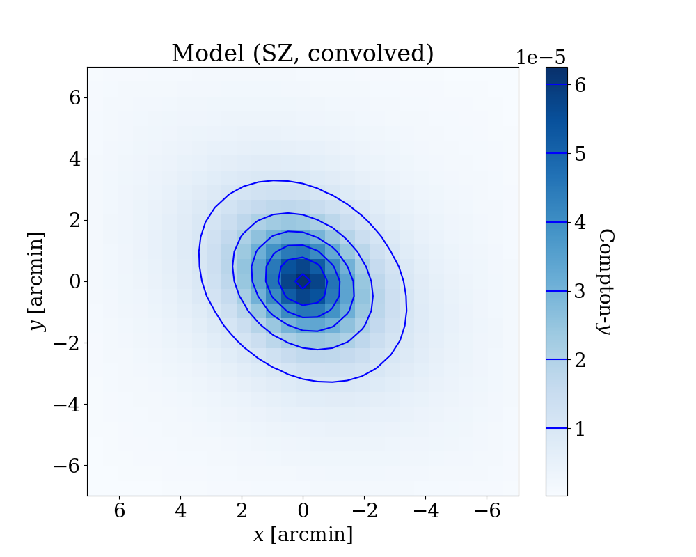
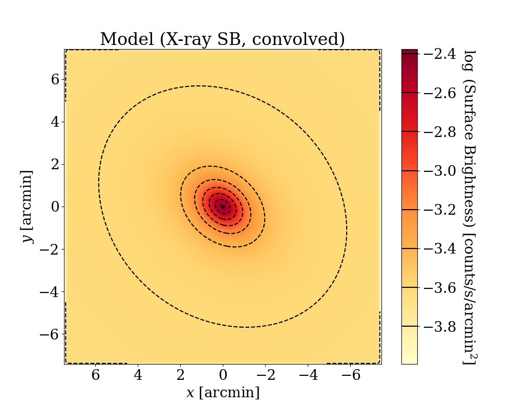
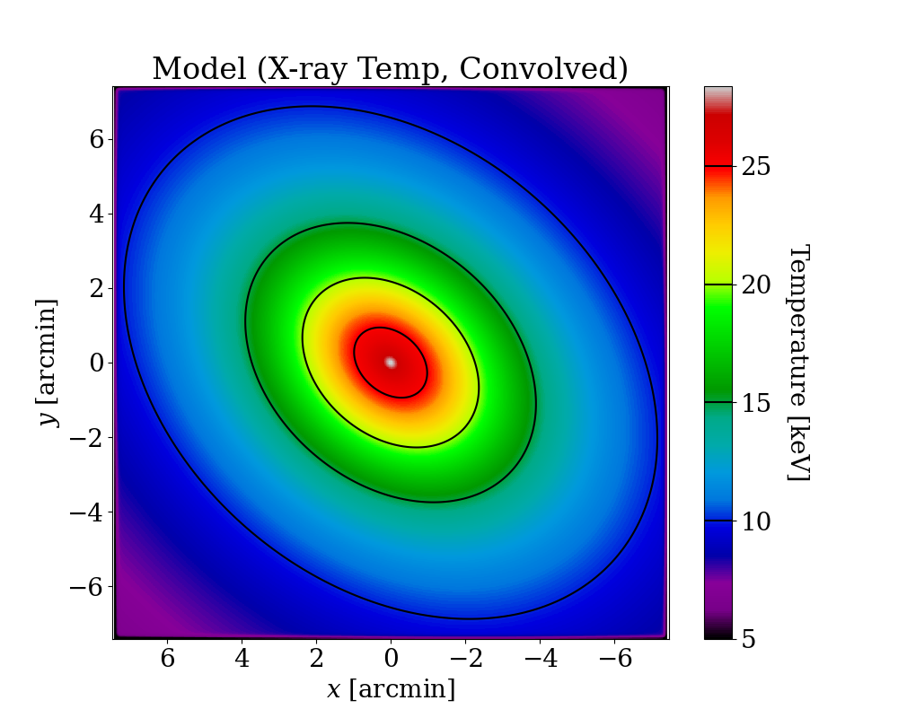
Figure 2: The projected, PSF-convolved SZ model map (left). PSF convolved, X-ray surface brightness (middle) and temperature (right) maps. The contours for the models are overlaid to improve the visual representation of the maps. The simulated PSFs used for the SZ and X-ray maps correspond to 7′ and 10″ FWHM, respectively. To ensure accurate PSF convolution, we bin the pixels in the maps such that the FWHM of each instrument’s PSF is covered by at least three pixels.

To validate the accuracy of our model fitting algorithm, we conduct a full analysis using mock observations of a galaxy cluster described by our model from known input parameter values. Using the model parameters outlined in Table 1, we generate model SZ, X-ray SB and temperature maps, incorporating the instrument PSF response. For this test, we assume the mock cluster has the following characteristics: $z=0.18$, $M_{500}=8.8\times 10^{14}\textrm{M}_{\odot}$, $R_{500}=7.4$′. Additionally, we take the following values for the geometric configuration and electron density and pressure parameters, with $(q_{\text{\tiny ICM,1}},q_{\text{\tiny ICM,2}},\cos\theta,\varphi,\psi)=(0.6,0.75,0.8,-25,60)$, $(n_{0},\zeta_{\text{\tiny c}},\zeta_{t},\beta_{e},\eta_{e},\gamma_{e})=(0.002,175,1.5,0.6,0.3,1.8)$, $P_{0},\alpha_{p}=(10.0,1.0)$. In this case, $e_{\parallel}$ = 1.02.

Figure 3: Posterior distributions estimated from our MCMC for a mock observation generated from a smooth model. Green vertical lines in each plot indicate the input parameters used to generate the mock observation maps, while the red vertical lines represent the median value from the accepted MCMC samples. The values displayed above each histogram show the median of the distribution, along with the 1$\sigma$ (68.3%) credible region, which is indicated by dashed vertical lines in every plot. Additionally, the solid black line in the 2D distributions encloses the 68% credible region for the parameter pairs. As highlighted by Vikhlinin et al. (2006) and Nagai et al. (2007), there exists a correlation among the model parameters related to the ICM radial profiles, and individual parameter values exhibit degeneracy. However, our objective is to ascertain smooth analytic functions that accurately represent the electron density and pressure profiles, thereby providing a comprehensive description of the ICM thermodynamics.

The model maps generated with the input parameters are presented in Fig. 2. For each pixel based on its coordinates within the observed map, we calculate the observables projected onto the two-dimensional sky plane (Sec. 2.3). Then, instrumental effects, including the PSF response, are applied. As we discuss in the next section, our baseline analysis of the observed data uses the combined Planck and ACT SZ effect map (Aiola et al., 2020), and we assume a PSF with a FWHM of 1.6′. To ensure adequate angular sampling of the PSF, we require a maximum pixel size equal to the FWHM divided by three.

In addition, we incorporated noise into each mock observation. Using the error maps for the observed data, we randomly sampled Gaussian noise distributions for the SZ, X-ray SB, and X-ray temperature maps, respectively. Figure 3 shows the posterior distribution of the parameters from our fit to this mock observation. The posterior distributions indicate that we can accurately recover most of the varied parameter values within the expected deviations due to noise fluctuations. Thus, our fitting methodology is able to reliably determine the underlying shape and thermodynamics of the observed mock galaxy cluster.

The use of both SZ and X-ray data in our analysis allows us to measure the three-dimensional geometry of the ICM distribution by constraining the elongation parameter (Sec. 2.1), since the two observational probes redundantly measure the thermodynamic properties of the gas along the line-of-sight. However, it should be noted that there may be degeneracies in determining cluster shape through this multi-probe approach depending on the relative orientation of the geometry, especially in inferring the geometric parameters of the 3D structure, as discussed in Sereno (2007). These degeneracies can cause bias in the recovered shape parameters along with multimodality in the posterior distributions. A further exploration of these degeneracies, in particular as they pertain to the observational data available for the CHEX-MATE sample, will be included in a subsequent paper in this series.

3 Application to CHEX-MATE Data

In this section, we introduce the X-ray and SZ data collected from our program. We apply the triaxial analysis technique to analyze a CHEX-MATE galaxy cluster PSZ2 G313.33+61.13 (Abell 1689), and the cluster serves as an illustrative example to demonstrate the method.

3.1 Data

Table 2 summarizes the SZ and X-ray data from CHEX-MATE available for our multiwavelength analysis of the ICM distribution. The foundation of our analysis is the 3 Msec XMM-Newton observing program CHEX-MATE (CHEX-MATE Collaboration et al., 2021), from which we have obtained two-dimensional X-ray SB and temperature maps produced using the Voronoi tessellation method (Cappellari & Copin, 2003; Diehl & Statler, 2006). The details of the image production are reported in Bartalucci et al. (2023) and Lovisari et al. (2023), and here we report briefly the main analysis steps.

Table 2: List of the X-ray and SZ observation data and instruments used for the analysis of PSZ2 G313.33+61.13.

Wavelength	Type	Instrument	Reference
X-ray	Surface brightness (SB)	XMM-Newton	Bartalucci et al. (2023)
X-ray	Temperature	XMM-Newton	Lovisari et al. (2023)
mm-wave	SZ $y$-map	Planck	Planck Collaboration et al. (2016b)
mm-wave	SZ $y$-map	ACT (ACTPol)	Madhavacheril et al. (2020)

The XMM-Newton observations of the clusters were obtained using the EPIC instrument (Strüder et al., 2001; Turner et al., 2001). To create the X-ray SB map, photon-count images in the [0.7-1.2] keV range were extracted from the data acquired using the MOS1, MOS2, and pn cameras on the instrument. The energy band was selected to optimize the contrast between the emission from the source and the background (Ettori et al., 2010). The images from all three cameras were combined to maximize the statistical significance while accounting for the energy-band responses. Additionally, the X-ray maps are instrumental-background subtracted and corrected for the exposure. Point sources are removed from the analysis (Ghirardini et al., 2019) by masking them with circular regions that appear as empty circular regions in the X-ray maps in Fig. 4. Furthermore, they are spatially binned to have at least 20 counts per bin using the Voronoi technique. X-ray temperature maps (Lovisari et al., 2023) were prepared in a similar manner for the data obtained in the [0.3-7] keV band, with background modeling (Lovisari & Reiprich, 2019) and spectral fitting performed. The fitting procedure to ascertain the temperature was done utilizing the XSPEC (Arnaud, 1996), which was employed to minimize the modified Cash statistics (Cash, 1979) with the assumption of Asplund et al. (2009) metallicity. Subsequently, Voronoi-binned maps were generated to achieve a high signal-to-noise ratio ($\sim$30) for each cell.

Planck SZ maps are available for all of the CHEX-MATE galaxy clusters by definition (Planck Collaboration et al., 2013; Pointecouteau et al., 2021). From these data we have generated a custom $y$-map using the Modified Internal Linear Component Algorithm (MILCA; Hurier et al., 2013) with an improved angular resolution of 7′ FWHM compared to the one publicly released by Planck with an angular resolution of 10′ FWHM (Planck Collaboration et al., 2016b). Also, ground-based SZ observations from cosmic microwave background (CMB) surveys, including the ACT and the South Pole Telescope (SPT; Bleem et al., 2022), as well as the Caltech Submillimeter Observatory (CSO)’s Bolocam galaxy cluster archive (Sayers et al., 2013), provide higher angular resolution data for a subset of CHEX-MATE clusters. Some of these ground-based data are currently publicly accessible, while others are slated for future release.

In this demonstration paper, we make use of the ACT SZ component-separated maps. The recent data release 4 (DR4) from the ACT provides component-separated maps, one of which is the SZ (Aiola et al., 2020; Madhavacheril et al., 2020). These maps were generated by analyzing data from a 2,100 square degree area of the sky, captured using the ACTPol receiver (Henderson et al., 2016) at 98 and 150 GHz. This data offers more than four times finer angular resolution compared to the Planck map. Then, the maps were jointly analyzed and combined with Planck data. Rather than using the noise estimate provided with these data, which is quantified as a two dimensional power spectral density, we instead follow an approach based on the recent analysis of similar joint ACT and Planck maps in Pointecouteau et al. (2021). Specifically, we randomly sample 10,000 maps, ensuring that their size aligns with that of the input SZ data, in the corresponding ACT region (for instance, the region designated as ‘BN’ for the cluster Abell 1689 analyzed in the next section). Then, we compute the covariance using these maps to estimate the noise covariance matrix. The resulting noise rms for the $y$-map is approximately $\sim 9\times 10^{-6}$ per 0.5′ square pixel, and the diagonal elements of the noise covariance matrix are shown along with the $y$-map in Fig. 4.

3.2 PSZ2 G313.33+61.13 (Abell 1689)

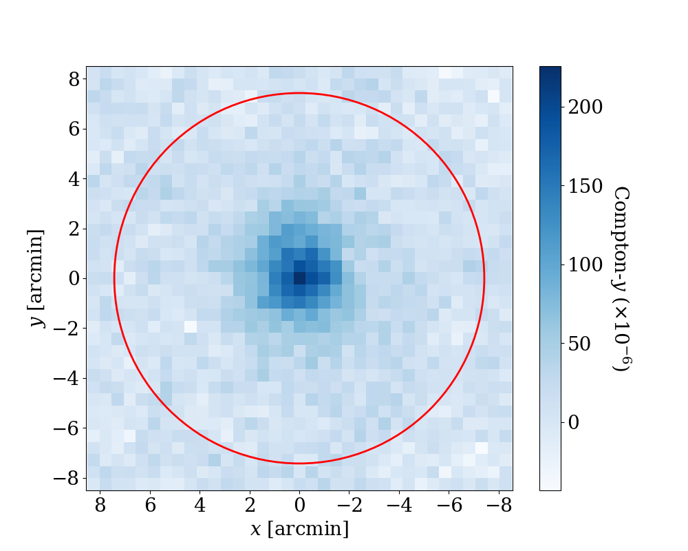
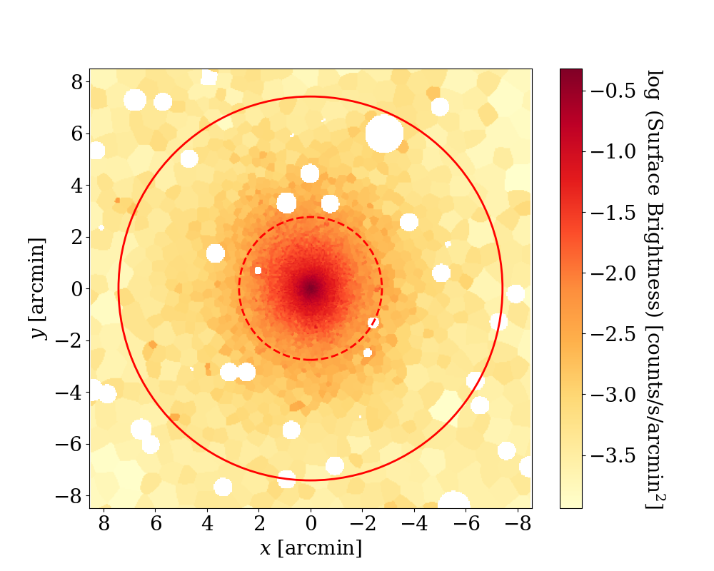
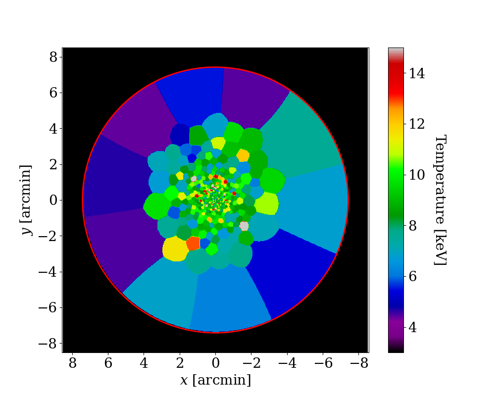
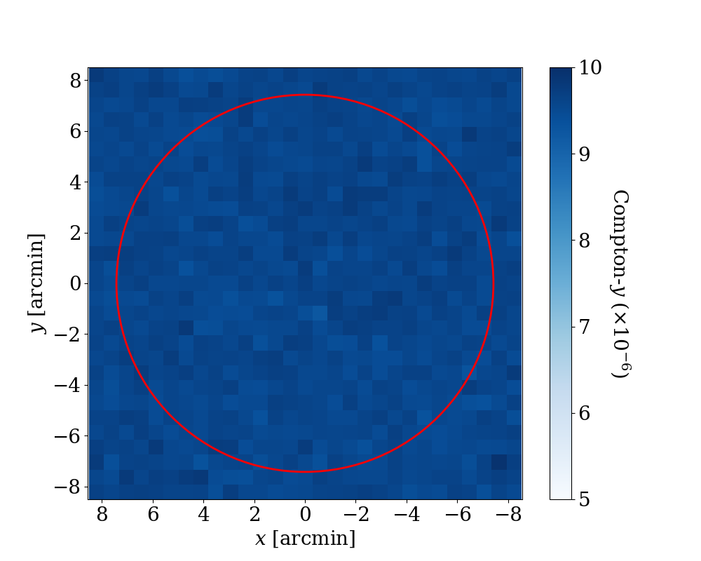
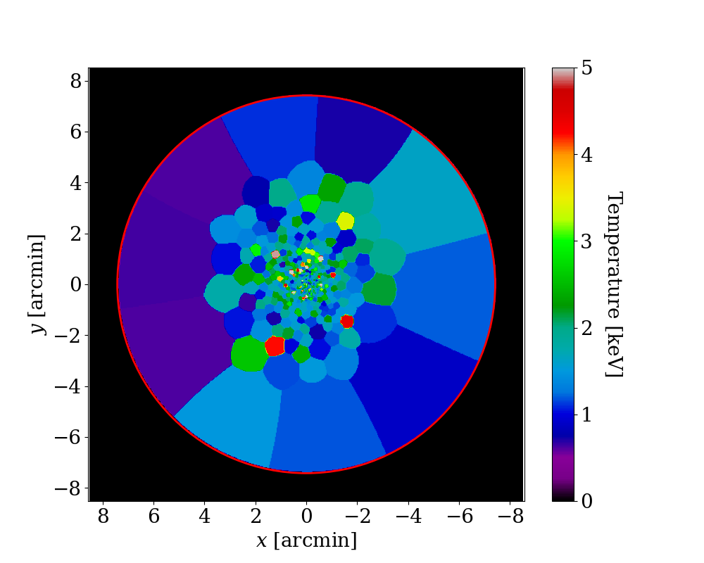
Figure 4: The SZ and X-ray maps of the CHEX-MATE galaxy cluster PSZ2 G313.33+61.13 (Abell 1689). The ACT Compton-$y$ map (top left) and its error (bottom left) map, the X-ray SB (top middle) and its error (bottom middle) map, and the X-ray temperature (top right) and its error (bottom right) map are shown. The ACT SZ map is one of the component-separated map products that were produced using the internal linear combination method and combined with data from the Planck (i.e., this is a joint map from ACT + Planck data, Madhavacheril et al. 2020). The X-ray maps are the data products of Bartalucci et al. (2023) and Lovisari et al. (2023). Bright point sources in the X-ray SB maps are indicated by white circles and masked in the analysis, and the same point-source regions are also removed from the spectral analysis to obtain the temperatures. The regions are excluded in the model fit. The X-ray SB maps are binned using a Voronoi algorithm to ensure an adequate number of photon counts per bin, with smaller bin sizes used in the central region where the count rates are higher. For the temperature maps, Voronoi binning was similarly applied using a fixed signal-to-noise ratio of 30 instead of a fixed number of counts, ensuring a roughly uniform statistical uncertainty per bin. In the X-ray and SZ maps, red circles indicate the two-dimensional map regions included in our analysis. We incorporate a circular region with a radius of $r=R_{500}$ around the galaxy cluster center for the SZ and the X-ray data by applying a circular mask to the maps, and the radius is shown as red circles. For this particular cluster, $R_{500}$ is equal to 7.42′ ($\sim$1.37 Mpc). In the X-ray SB and its corresponding error maps, red dashed circles represent the region that encompasses 80% of the emission in the SB map, which is where the 2D (inner region) and 1D analyses (outer region) are separated, and it is located at $r=2.58$′. We will explore and implement a comparable approach that integrates both 2D and 1D analysis techniques for temperature data, as described by Lovisari et al. (2023), in a forthcoming analysis.

Using the datasets described above, we demonstrate our fitting method for PSZ2 G313.33+61.13 (Abell 1689), which is a Tier-2 cluster in the CHEX-MATE sample located at $z=0.1832$ with a Planck SZ estimated mass of $M_{500}=8.77\times 10^{14}\textrm{M}_{\odot}$. We note the lensing mass measurement of the cluster is $\sim$70% higher than the Planck hydrostatic mass estimate; see Umetsu et al. (2015). We conducted a triaxial fit aligning the model center with the X-ray peak (Bartalucci et al., 2023). For a morphologically regular cluster, like Abell 1689, any deviations or offsets between the SZ and X-ray measurements are expected to have minimal impact on the overall model fit. The Planck + ACT SZ $y$-maps, along with the XMM-Newton X-ray SB and temperature maps, are shown in Fig. 4. Maps of the rms noise for each observable are also included, and indicate that the cluster is imaged at high signal to noise. This particular cluster was chosen for our demonstration because its triaxial shape has been well studied in the literature (Morandi et al., 2011; Sereno & Umetsu, 2011; Sereno et al., 2012; Umetsu et al., 2015). For example, Sereno et al. (2012) performed a gas-only analysis using radial profiles of the X-ray and SZ observations from Chandra, XMM-Newton  WMAP, along with various ground-based SZ facilities, and constrained the shape and orientation of the cluster’s triaxial model with $q_{\text{\tiny ICM,1}}=0.70\pm 0.15$, $q_{\text{\tiny ICM,2}}=0.81\pm 0.16$, and $\cos\theta=0.70\pm 0.29$. A subsequent study by Umetsu et al. (2015) presented a combined multiwavelength analysis that included lensing data, with the inferred ICM distribution being $q_{\text{\tiny ICM,1}}=0.60\pm 0.14$, $q_{\text{\tiny ICM,2}}=0.70\pm 0.16$. Their derived value of $\cos\theta$, obtained from the combined lensing and X-ray/SZ analysis, was found to be $0.93\pm 0.06$. The large $\cos\theta$ suggests that the major axis of the triaxial ellipsoid ($x^{\text{\tiny int}}_{3}$ in Fig. 1) is closely aligned with the observer’s line of sight.

Table 3: Parameters describing the triaxial geometry of PSZ2 G313.33+61.13 (Abell 1689)

$q_{\text{\tiny ICM,1}}$	$q_{\text{\tiny ICM,2}}$	$\cos\theta$	$e_{\parallel}$	Reference
$0.70\pm 0.15$	$0.81\pm 0.16$	$0.70\pm 0.29$	$1.68\pm 0.53$	Sereno et al. (2012)
$0.60\pm 0.14$	$0.70\pm 0.16$	$0.93\pm 0.06$	$1.16\pm 0.10$	Umetsu et al. (2015)
$0.65\pm 0.02$	$0.79\pm 0.02$	$\geq 0.96$	$1.24\pm 0.03$	This work

Figure 5: The posterior distribution of the model fit parameters for the galaxy cluster PSZ2 G313.33+61.13 obtained using SZ data from Planck and ACT, as well as X-ray data from XMM-Newton. The red vertical lines indicate the median value from the accepted MCMC samples, with values displayed along with their 68% credible regions above each histogram. Instead of the Euler angles $\varphi$ and $\psi$, we present $e_{\parallel}$, which is a function of five geometric parameters of a triaxial ellipsoid (Eq. 6).

Figure 5 shows the posterior of the model parameters that describe our triaxial fit of PSZ2 G313.33+61.13, using the data from Planck, ACT, and XMM-Newton. We find axial ratios of $q_{\text{\tiny ICM,1}}=0.65\pm 0.02$ and $q_{\text{\tiny ICM,2}}=0.79\pm 0.02$. These values are consistent with previous results, but an order of magnitude more precise (Table 3). Our fits indicate the major axis of Abell 1689 is almost perfectly aligned with the line of sight, with $\cos\theta\geq 0.96$ at 90% confidence. While previous works also indicated such an alignment, a much wider range of orientations were allowed in those fits. We note that our analysis only includes statistical uncertainties on the fit, and the uncertainty due to data calibration is not taken into account here. Also, as the elongation parameter (Eq. 6), which is the ratio of the size of the ellipsoid along the observed line-of-sight to the major axis of the projected ellipse in the sky plane, quantifies the 3D geometry of the triaxial ellipsoid model of the ICM. We thus present constraints on $e_{\parallel}$ rather than on $\varphi$ and $\psi$. The inferred $e_{\parallel}$ is well constrained in the fit to a value of $1.24\pm 0.03$ and is consistent with the gas analysis result of Sereno et al. (2012), who found $e_{\triangle}=0.66\pm 0.21$, which corresponds to $1.15\leq e_{\parallel}\leq 2.22$. Figure 6 shows the reconstructed SZ, X-ray SB and temperature maps of PSZ2 G313.33+61.13, incorporating the instrument response, generated using the recovered parameters from Fig. 5. The difference map, which is created by taking the input data and subtracting the reconstructed model from it, reveals that the majority of the pixels exhibit relative errors that are spread within a range of $\pm 4\sigma$ (Fig. 5). The residuals for the SZ, X-ray SB, and X-ray temperatures are distributed around zero. Their respective standard deviations are equivalent to $1.5\sigma$, $0.6\sigma$, and $1.1\sigma$ when fitted by a Gaussian.

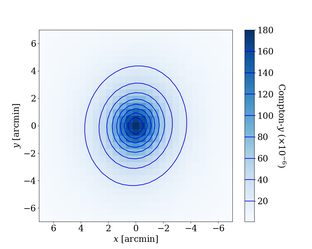
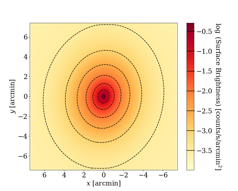
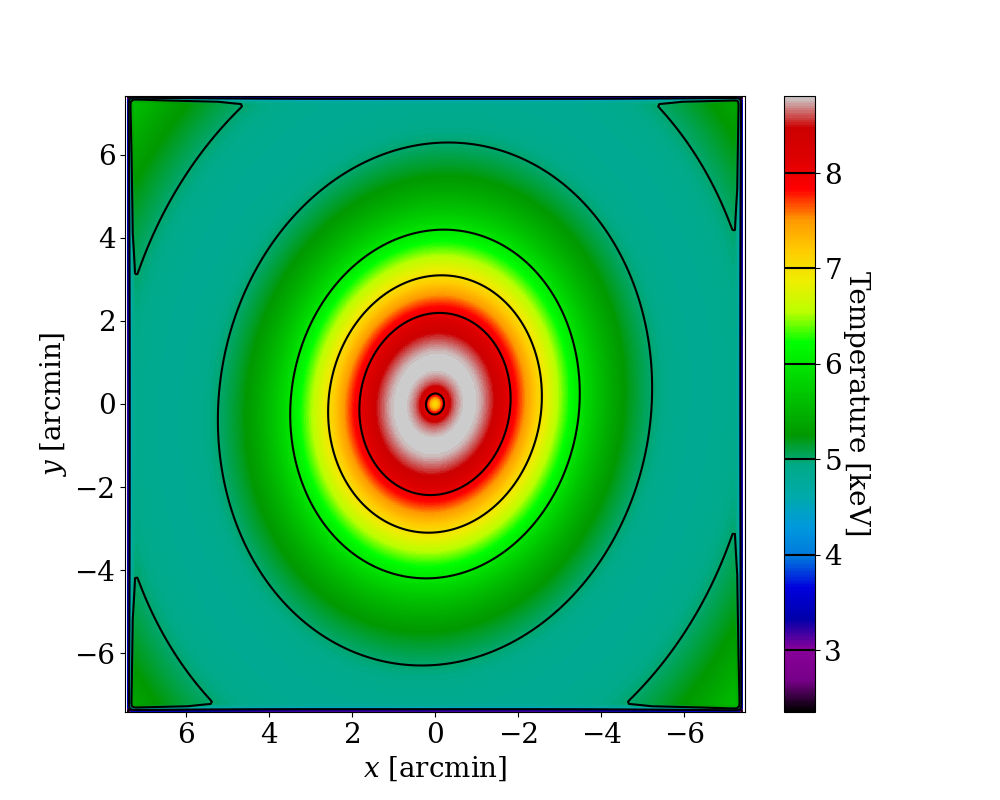
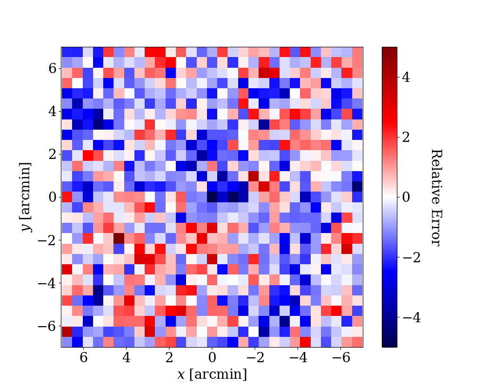
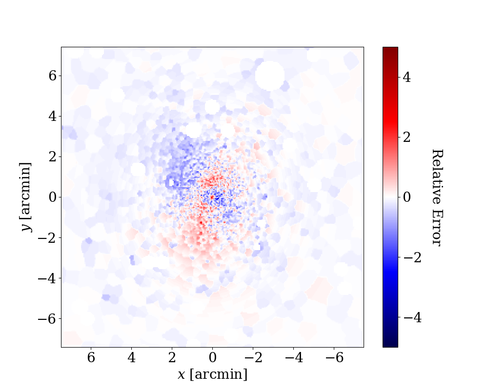
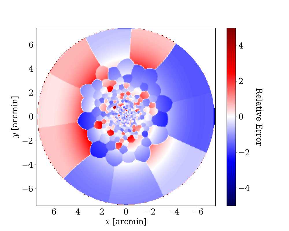
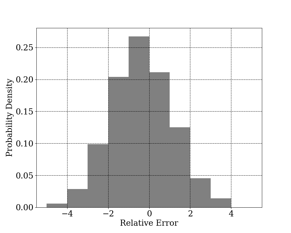
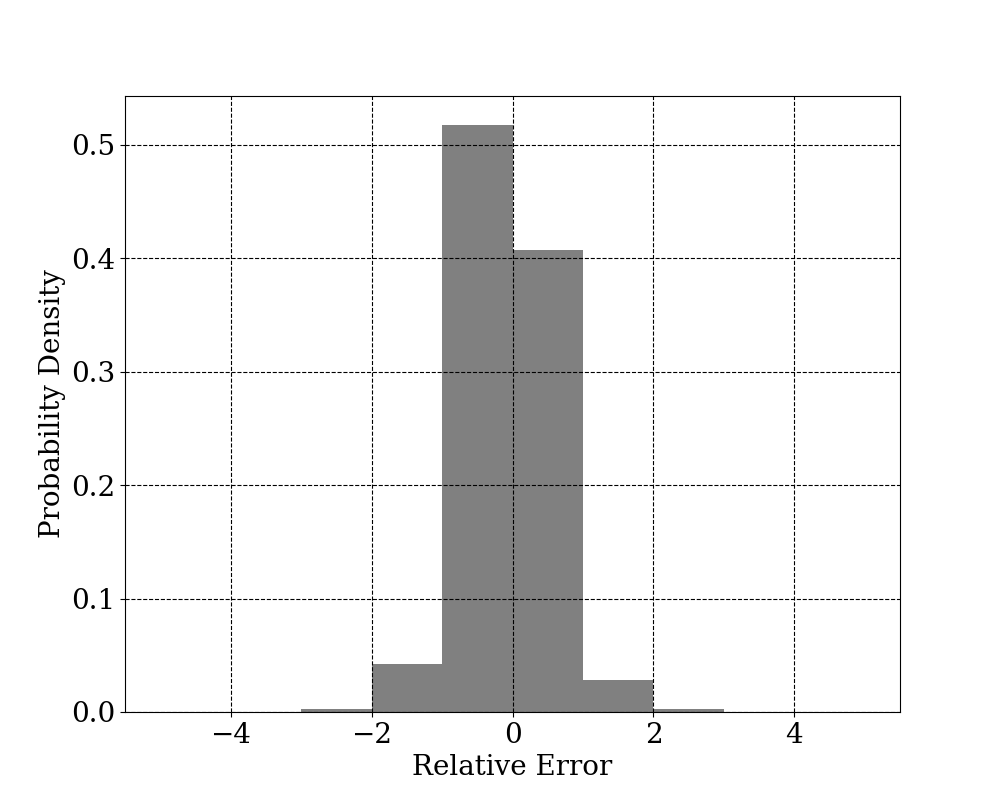
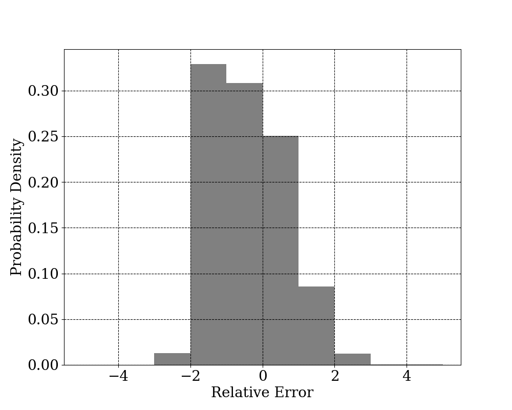
Figure 6: Reconstructed SZ and X-ray models of PSZ2 G313.33+61.13 generated using the recovered parameters from Fig. 5 (top). The difference between the observational data and the reconstructed model map above, in units of pixel-based error (middle). The histogram of the distribution of the relative error in the middle panels (bottom). The X-ray SB histogram takes into account both the residuals in the inner 2D region, which includes 80% of the emissions observed in the data, and the outer map region where we implemented 1D analysis using azimuthal medians (see Fig. 4). In all cases, the residuals are distributed within $\pm 4\sigma$ level compared to the error. When the relative errors of the SZ, X-ray SB, and X-ray temperature are modeled with a Gaussian fit, their standard deviations align with $1.5\sigma$, $0.6\sigma$, and $1.1\sigma$ respectively.

For comparison, we performed an additional X-ray + SZ fit using only the Planck SZ data, without incorporating the ground-based ACT data. We obtain posteriors that significantly deviate from our baseline fit with ACT data. We attribute this to the coarse angular resolution of Planck  which prevents it from resolving morphological features given the angular size of Abell 1689 at z=0.1832. To test this, we generated two sets of mock observations using the recovered parameters from our baseline fit to the observed data from both Planck and ACT (along with XMM-Newton). One mock was based on the properties of the $y$-map from Planck + ACT, while the other mimicked the $y$-map with only Planck SZ data, including the appropriate noise and PSF shape for each case. Our fit to the mock multiwavelength data with the Planck + ACT $y$-map yields recovered parameters closely aligned with the input model, suggesting these data can accurately recover the input ICM shape. In contrast, the second mock observation based on the Planck-only $y$-map produces a set of parameters significantly deviating from the input. This suggests that the SZ data from Planck alone are insufficient to reliably fit our triaxial model, at least for a galaxy cluster with this specific shape at this specific redshift. This confirms that our fit to observed data using the Planck-only $y$-map are likely biased. In a subsequent paper we will explore this issue in more detail, to better understand which types of galaxy clusters can (or cannot) be reliably reconstructed with the data available for CHEX-MATE.

Furthermore, in order to evaluate how the much higher overall signal to noise of the X-ray SB compared to the SZ and X-ray temperature impacts the results, we carried out an additional fit using the reduced $\chi^{2}$ for each of the three observables in order to weight them equally in the fit. The results of this fit indicate that there is only a minimal shift in the values of the derived geometric parameters based on this equal weighting of the three observables. Specifically, in the reduced $\chi^{2}$ fit, $q_{\text{\tiny ICM,1}}$ has a value of $0.70\pm 0.04$, $q_{\text{\tiny ICM,2}}$ is $0.78\pm 0.05$, and $e_{\parallel}$ stands at $1.22\pm 0.07$. We also attempted to account for fluctuations in the calibration uncertainty, which can be especially important for the temperature profile (e.g., Schellenberger et al., 2015; Wallbank et al., 2022). We conducted model fits by introducing an additional $\sim 10\%$ uncertainty of the temperature, but observed little changes in the parameters, with posteriors displaying similar levels of variation.

As we will illustrate in subsequent studies, the derived geometric parameters of the ICM distribution, such as the elongation that quantifies the 3D geometry, can be applied in conjunction with gravitational lensing measurements. For these fits, we will work under the assumption that the triaxial axes of the ICM and dark matter are coaligned, but with axial ratios that are allowed to vary. The lensing analysis becomes crucial for discerning the triaxial shapes of dark matter, circumventing the need to rely on hydrostatic equilibrium or simulation-based corrections. Consequently, a comprehensive multi-probe analysis facilitates a characterization of the total matter distribution, which is essential for precise lensing-based mass calibrations (Sereno et al., 2018), along with allowing for a determination of the distribution of non-thermal pressure support (Sayers et al., 2021).

4 Conclusions

We have improved a multi-probe analysis package to fit the three-dimensional ellipsoidal shapes of CHEX-MATE galaxy clusters. This package builds upon CLUMP-3D (Sereno et al., 2017), which was employed to analyze the triaxial shapes of CLASH clusters (Sereno et al., 2018; Chiu et al., 2018; Sayers et al., 2021). Specifically, we have made the following improvements: 1) we model 2D distributions of the SZ and X-ray temperature data, in contrast to the 1D azimuthally averaged profiles in these quantities used by Sereno et al. (2017), 2) we parametrize electron density and pressure rather than density and temperature, reducing the number of parameters and speeding up the fit, and 3) we have ported the code to Python to facilitate a future public release. For the two-dimensional map analyses, we have added the capability to include publicly available SZ data from ground-based CMB surveys such as ACT, in addition to the default Planck SZ maps.

We verified the triaxial analysis method through mock data analysis and applied it to the actual CHEX-MATE galaxy cluster, PSZ2 G313.33+61.13 (Abell 1689). The analysis effectively constrains the model geometry, in particular, at the few percent level for the axial ratios. Our results are consistent with previous analyses of Abell 1689 available in the literature. Specifically, we find axial ratios of $q_{\text{\tiny ICM,1}}=0.65\pm 0.02$, $q_{\text{\tiny ICM,2}}=0.79\pm 0.02$, and elongation parameter $e_{\parallel}=1.24\pm 0.03$. Compared to the similar gas-only analysis using X-ray and SZ data presented in Sereno et al. (2012), the axial ratios and elongation parameters in our study demonstrate a substantial improvement, with uncertainties an order of magnitude lower. This marked improvement is attributable to multiple factors: our use of deeper new XMM-Newton data not available to Sereno et al. (2012); our use of an XMM-Newton SB image rather than a shallower Chandra SB image; our use of much higher quality SZ data from Planck and ACT rather than from WMAP and SZA/OVRO/BIMA; and our improved analysis formalism making use of fully 2D images for all of the observables rather than a projected elliptically averaged profile of X-ray SB and temperature along with a single aperture photometric measurement of the SZ signal. Our results indicate that Abell 1689 has axial ratios typical of what is expected for the general population of galaxy clusters (Jing & Suto, 2002; Lau et al., 2011), but a remarkably close alignment between the major axis and the line of sight. This alignment has resulted in exceptional lensing properties of Abell 1689, such as an abundance of strong lensing features (e.g., Broadhurst et al., 2005; Limousin et al., 2007), one of the largest Einstein radii observed (47″, Coe et al., 2010), and an extremely large concentration for its mass when fitted to a spherically symmetric model ($c_{\textrm{vir}}=12.8^{+3.1}_{-2.4}$ or $c_{200}=10.2^{+2.6}_{-1.9}$, Umetsu et al., 2011; Umetsu, 2020). We thus conclude that there is nothing unusual about the triaxial shape of Abell 1689, other than its orientation. In addition, the estimated axial ratios of the cluster yield a triaxiality parameter $t=0.66$ (Franx et al., 1991). While the incorporation of lensing data is necessary for a direct quantitative comparison with DM axial ratios, the calculated $t$ classifies this halo as being close to the ‘prolate’ population that comprises $\sim\!80$% of the total cluster fraction in the DM only simulations (Vega-Ferrero et al., 2017). The integration of lensing data for a comprehensive multi-wavelength analysis, as well as the public release of the software and data products, will be addressed in subsequent papers of this series.