Anomalous Andreev Spectrum and Transport in Non-Hermitian Josephson Junctions

Abstract

We propose a phase-biased non-Hermitian Josephson junction (NHJJ) composed of two superconductors mediated by a short non-Hermitian link. We find that its Andreev spectrum as a function of phase difference exhibits Josephson gaps, i.e. finite phase windows, in which Andreev quasi-bound states do not exist. Remarkably, exceptional points emerge in the complex Andreev spectrum, constituting a particular spectral feature of NHJJs. Moreover, we propose complex supercurrents due to inelastic Cooper pair tunneling. At the exceptional points, the corresponding phase-biased supercurrent divergences. Our results illustrate that the Josephson effect is strongly affected by non-Hermitian physics.

Introduction.—In recent years, there has been growing interest in non-Hermitian systems Bender (2007); El-Ganainy et al. (2018); Ashida et al. (2020); Bergholtz et al. (2021); Okuma and Sato (2023). Non-Hermitian physics emerges in a variety of fields such as disordered systems Zyuzin and Zyuzin (2018); Papaj et al. (2019), correlated solids Yoshida et al. (2019); Nagai et al. (2020), and open or driven systems Makris et al. (2008); Guo et al. (2009); Rotter (2009); Nakagawa et al. (2018); Xiao et al. (2019); Li et al. (2019); Zhang and Gong (2020). Different from the Hermitian case, the eigenvalues of non-Hermitian systems are complex in general. The complex-valued nature of the spectrum gives rise to unique features such as exceptional points Dembowski et al. (2001); Berry (2004); Kawabata et al. (2019a), point gaps Kawabata et al. (2019b); Zhou and Lee (2019), and enriched topological phases Lee (2016); Yao and Wang (2018); Kunst et al. (2018); Gong et al. (2018). Many of these particular phenomena have been theoretically studied and experimentally observed Lee (2016); Yao and Wang (2018); Kunst et al. (2018); Gong et al. (2018); Zhou and Lee (2019); Kawabata et al. (2019b, a); Zhang et al. (2020); Okuma et al. (2020); Yao et al. (2018); Leykam et al. (2017); Shen et al. (2018); Yin et al. (2018); Yokomizo and Murakami (2019); Lee and Thomale (2019); Longhi (2019); Lee et al. (2019); Yamamoto et al. (2019); Borgnia et al. (2020); Budich and Bergholtz (2020); Yamamoto et al. (2021); Franca et al. (2022); Cayao and Black-Schaffer (2022); Jezequel and Delplace (2023); Qin et al. (2023); Guo et al. (2023); Cayao and Black-Schaffer (2023); Sun et al. (2023); Li et al. (2022); Kornich (2023); Zeuner et al. (2015); Ding et al. (2016); Xiao et al. (2020); Ozturk et al. (2021); Liang et al. (2022); Zhang et al. (2023); Liang et al. (2023); Xu et al. (2023). Whereas the research on characterizing novel non-Hermitian systems has achieved impressive progress, the impact of non-Hermiticity on quantum transport is largely unexplored despite some related efforts Zhu et al. (2016); Longhi (2017); Chen and Zhai (2018); Bergholtz and Budich (2019); Shobe et al. (2021); Michen and Budich (2022); Kornich and Trauzettel (2022); Sticlet et al. (2022); Geng et al. (2023); Isobe and Nagaosa (2023), especially for the cases involving superconductivity. For instance, an intriguing open question is how non-Hermiticity affects low-energy spectral features of superconducting systems and results in particular transport signatures.

The best settings to study superconducting transport are Josephson junctions (JJs). Generally, JJs consist of two superconductors separated by a (weak) link Likharev (1979); Beenakker (1992); Golubov et al. (2004); Tinkham (1996). Hermitian JJs have been extensively studied for decades. Phase-coherent quantum transport in Hermitian JJs gives rise to the dc Josephson effect: a phase-dependent supercurrent without voltage bias. In the short junction regime, the Josephson effect is entirely determined by the low-energy Andreev spectrum Furusaki (1999); Beenakker and van Houten (1991); Kwon et al. (2004); Fu and Kane (2009); Dolcini et al. (2015); Beenakker et al. (2013). When non-Hermiticity is introduced, we expect that the impact of non-Hermiticity on fundamental properties of JJs, such as the low-energy Andreev spectrum and the phase-biased supercurrent, is substantial. Moreover, it is also of high experimental relevance because JJs are always coupled to the environment and non-Hermitian parts of a Hamiltonian mimic certain aspects of this coupling.

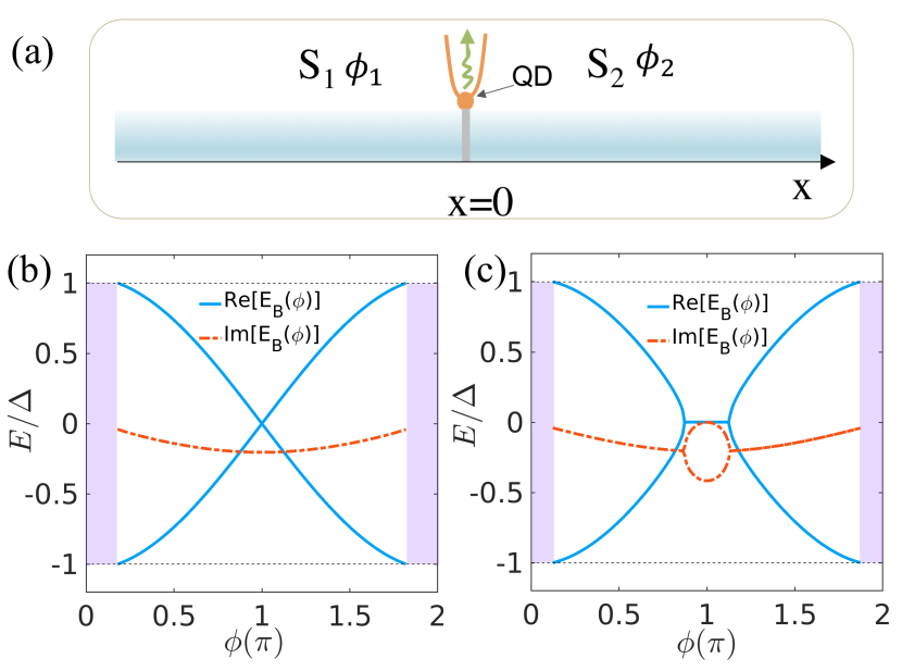
FIG. 1: (a) Sketch of a 1D NHJJ: two superconductors are connected by a short junction, which is coupled to the environment (a reservoir and a quantum dot (QD)). The QD is used to monitor the tunneling of quasiparticles between system and reservoir. The superconductors can either be of $s$-wave or $p$-wave type. The two superconductors possess a phase difference $\phi=\phi_{1}-\phi_{2}$. The wavy line indicates loss due to the coupling to the environment. (b) Complex Andreev spectrum as a function of $\phi$ within the superconducting gap $\Delta$ in the $s$-wave NHJJ. The purple regions indicate Josephson gaps. (c) Complex Andreev spectrum as a function of $\phi$ in the $p$-wave NHJJ. A pair of exceptional points appear, implying unique non-Hermitian spectral features. We choose $Z=0.2$ for the non-Hermitian barrier strength in (b) and (c).

In this work, we investigate the low-energy spectrum and transport properties of a short non-Hermitian Josephson junction (NHJJ). The proposed NHJJ is built up of two superconductors connected by a non-Hermitian barrier [Fig. 1(a)]. We discover that the Andreev spectrum becomes complex-valued and exhibits Josephson gaps [purple regions in Figs. 1(b) and 1(c)]. Due to the complex-valued nature of Andreev spectrum, the supercurrent becomes complex. Its imaginary part signifies the loss of quasiparticles due to inelastic Cooper pair tunneling. Remarkably, we find that the complex Andreev spectrum of $p$-wave NHJJs hosts a pair of exceptional points (EPs) [Fig. 1(c)]. At these EPs, the corresponding supercurrent diverges, promoting the sensitivity of JJs extensively. We also perform detailed tight-binding calculations to simulate experimental implementations of our proposal.

Effective non-Hermitian Hamiltonian of the NHJJ.—We consider a minimal one-dimensional (1D) NHJJ as sketched in Fig. 1(a). The junction is coupled to a fermionic environment, constituting an open quantum system. We derive an effective NH Hamiltonian description for this system from the Lindblad formalism under certain approximations Breuer and Petruccione (2002); Daley (2014); Minganti et al. (2019); Manzano (2020); Roccati et al. (2022) in the Supplemental Material (SM) Li2 (a). This results in an imaginary potential at the junction, i.e.

$$U(x)=-iV\delta(x),\ V>0,$$ (1)

representing the continuous loss of quasiparticles and coherence from the system into the environment Breuer and Petruccione (2002); Nazarov and Blanter (2006); Daley (2014); Minganti et al. (2019). The strength $V$ measures the magnitude of the loss.

The Bogoliubov-de Gennes (BdG) Hamiltonian to describe the NHJJ can be written as

$$\mathcal{H}_{\mathrm{BdG}}=\left(\begin{array}[]{cc}-\frac{\hbar^{2}\partial_{x}^{2}}{2m}-\mu+U(x)&\hat{\Delta}(x)\\ \hat{\Delta}^{\dagger}(x)&\frac{\hbar^{2}\partial_{x}^{2}}{2m}+\mu+U(x)\end{array}\right),$$ (2)

where $m$ is the effective mass of the electrons, $\mu$ the chemical potential, and $\hat{\Delta}(x)$ the pairing potential which can be either of $s$-wave or $p$-wave type. We argue that the particle-hole symmetry of the type $U\mathcal{H}_{\mathrm{BdG}}^{*}U^{-1}=-\mathcal{H}_{\mathrm{BdG}}$ is physically relevant in our model Li2 (a), where $U$ is a unitary matrix. Note that this particle-hole symmetry is labeled as $\mathrm{PHS}^{\dagger}$ in the literature Kawabata et al. (2019a, b). Considering the energy spectrum of the system, electron and hole excitations are described by the BdG equation $\mathcal{H}_{\mathrm{BdG}}\psi(x)=E\psi(x)$, where the eigenstate $\psi(x)=(u(x),v(x))^{T}$ is a mixture of electron and hole components, and $E$ is the excitation energy measured relative to the Fermi energy. The eigenenergy of $\mathcal{H}_{\mathrm{BdG}}$ always comes in pairs $E\longleftrightarrow-E^{*}$ under $\mathrm{PHS}^{\dagger}$.

Andreev quasi-bound states.—We now consider an $s$-wave NHJJ, in which the two superconductors are both of $s$-wave type. Without loss of generality, we assume that left and right superconductors have a constant pairing potential of the same magnitude but different phases, i.e., $\hat{\Delta}(x<0)=\Delta$ and $\hat{\Delta}(x>0)=\Delta e^{i\phi}$ where $\phi$ is the phase difference across the junction. We are interested in the low-energy bound states existing within the superconducting gap. We obtain such Andreev quasi-bound states in the NHJJ by solving the BdG equation with proper boundary conditions Furusaki and Tsukada (1991); Beenakker (1991). The bound states decay exponentially for $|x|\rightarrow\infty$ with a finite decay length $\lambda$. Therefore, the necessary condition for the existence of a bound state is given by $\mathrm{Re}(\lambda)>0$ with $\lambda=\frac{\hbar v_{F}}{\Delta}\frac{1}{\sqrt{1-E_{B}^{2}/\Delta^{2}}}$, where $v_{F}$ is the Fermi velocity.

The secular equation to determine the energy of Andreev quasi-bound state is Li2 (a)

$$(Z^{2}+1)+2iZ\sqrt{\Delta^{2}/E_{B}^{2}-1}=\Delta^{2}[Z^{2}+\cos^{2}(\frac{\phi}{2})]/E_{B}^{2}.$$ (3)

The strength parameter $Z$ for the NH barrier potential is defined as $Z\equiv\frac{mV}{\hbar^{2}k_{F}}$, where $k_{F}$ is the Fermi wavevector. Noticing the imaginary term $2iZ\sqrt{\Delta^{2}/E_{B}^{2}-1}$ in Eq. (3), the Andreev spectrum can be complex different from the Hermitian case Furusaki (1999); Beenakker and van Houten (1991); Kwon et al. (2004); Fu and Kane (2009); Dolcini et al. (2015); Beenakker et al. (2013). At $Z=0$, it reduces to the Kulik-Omel’yanchuk (KO) limit $E_{B}^{\pm}(\phi)=\pm\Delta\cos(\frac{\phi}{2})$ for a bare JJ Kulik and Omel’yanchuk (1975). For $Z\gg 1$, the spectrum becomes $E_{B}^{\pm}(\phi)=\pm\Delta$, merging with the continuum. The dimensionless parameter $Z$ can be estimated as $Z\sim\frac{\Gamma L}{\hbar v_{F}}$, where $\Gamma$ is the loss rate and $L$ is the junction length. Considering an experimental setup with feasible dimensions, $Z$ is estimated to be of the order of $Z\sim 10^{-1}$ . We focus on this experimentally relevant regime of $Z$ below.

At special values $\phi=2n\pi$ with integer $n$, a trivial solution $E_{B}^{\pm}(\phi=2n\pi)=\pm\Delta$ is possible, merging with the continuum. At $\phi=(2n+1)\pi$, we find that the Andreev spectrum is purely imaginary taking $E_{B}^{\pm}[(2n+1)\pi]=\frac{-iZ\Delta}{\sqrt{1-Z^{2}}}$, consistent with constraint on the spectrum from $\mathrm{PHS}^{\dagger}$. For general phase difference $\phi\in[\phi_{b},\phi_{t}]$, the secular equation implies

$$\frac{E_{B}^{\pm}(\phi)}{\Delta}=\frac{\pm\zeta\cos(\frac{\phi}{2})-iZ\sqrt{\sin^{2}(\frac{\phi}{2})-Z^{2}}}{1-Z^{2}},$$ (4)

with the sign function $\zeta=\mathrm{sgn}[\cos(\frac{\phi}{2})]$. We plot the corresponding Andreev spectrum in Fig. 1(b). The real part of the complex Andreev spectrum indicates the physical energy while its imaginary part characterizes a finite lifetime of quasiparticles traveling across the junction. The phase boundaries are $\phi_{b}\equiv 2n\pi+\phi_{0}(Z)$ and $\phi_{t}\equiv(2n+1)\pi-\phi_{0}(Z)$ with $\phi_{0}(Z)\equiv 2\arcsin(\sqrt{2}Z/\sqrt{1+Z^{2}})$. Note that Eq. (4) is only valid for $Z<1$. For $Z\geq 1$, there are no quasi-bound states in the junction anymore.

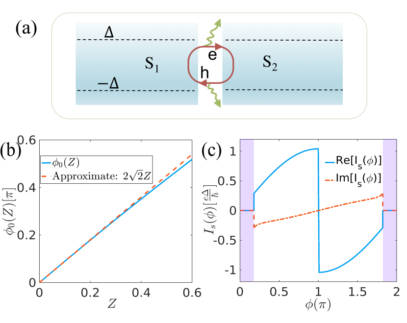
FIG. 2: (a) Sketch of inelastic Cooper pair tunneling. Transfer of Cooper pairs experiences possible decoherence and quasiparticles loss (wavy lines). (b) Josephson-gap phase boundary $\phi_{0}(Z)$ as a function of $Z$. (c) Complex supercurrents as a function of $\phi$ with $Z=0.2$.

Josephson gaps.—In general, the Andreev spectrum is a continuous function with respect to the phase difference $\phi$. However, we find that within a finite phase window $\Phi_{W}\equiv[2n\pi-\phi_{0}(Z),2n\pi+\phi_{0}(Z)]$ with $n\in\mathbb{Z}$, low-energy Andreev quasi-bound states are not allowed at all within the superconducting gap $\Delta$. We call such phase windows Josephson gaps. Its gap value is $2\phi_{0}(Z)=4\arcsin(\sqrt{2}Z/\sqrt{1+Z^{2}})$. For $Z\ll 1$, the Andreev spectrum can be approximated as $E_{B}^{\pm}(\phi_{0})\approx\Delta(\text{$\pm 1$}-iZ^{2})$ at the phase boundary $\phi_{0}(Z)$. The appearance of Josephson gaps can be understood as a consequence of the competition between phase-coherent transport of Cooper pairs across the junction and decoherence induced by the NH barrier . In the Hermitian case, due to phase coherence across the junction, quasiparticles move back and forth in the junction carrying the phase factor of superconductors imprinted by Andreev reflection Tinkham (1996); Nazarov and Blanter (2006); Golubov et al. (2004); Furusaki (1999). Andreev reflections lead to phase-coherent transport of Cooper pairs across the junction, i.e. the dc supercurrent. However, the NH mechanism in the NHJJ gives rise to loss of coherence and inelastic Andreev reflections [see Fig. 2(a) for a schematic] Nazarov and Blanter (2006); Daley (2014); Minganti et al. (2019). The magnitude of $Z$ determines the strength of decoherence. Hence, it is clear that the larger $Z$, the stronger is the coupling between system and environment. For phase differences $\phi\sim 0$ (mod $2\pi$) associated with a small supercurrent meaning a small number of transferred Cooper pairs, we observe Josephson gaps. This implies that phase-coherent transport of Cooper pairs is totally absent (thus no bound states). For larger supercurrents, i.e. larger phase differences, the pair breaking mechanism related to the barrier strength $Z$ is not sufficient to block the supercurrent. Nevertheless, decoherence modifies the supercurrent in this case. The Josephson-gap phase boundary $\phi_{0}(Z)$ depends on the value of $Z$. In Fig. 2(b), we plot the Josephson-gap phase boundary as a function of $Z$. It grows almost linearly with increasing $Z$. A numerical confirmation for the presence of Josephson gaps is presented in the SM Li2 (a).

Inelastic Cooper pair tunneling and complex supercurrent.—In (short) Hermitian JJs, the supercurrent originates from the coherent Cooper pair tunneling related to the Andreev spectrum Beenakker (1991, 1992); Furusaki (1999). In NHJJs, the Andreev spectrum becomes complex. The imaginary part of the Andreev spectrum indicates a finite lifetime of quasiparticles. Thus, the NH mechanism introduces loss of quasiparticles and decoherence during the Andreev reflection processes Breuer and Petruccione (2002); Nazarov and Blanter (2006); Daley (2014); Minganti et al. (2019) [see Fig. 2(a)], leading to inelastic Cooper pair tunneling  Devoret et al. (1990); Ingold and Nazarov (1994); Hofheinz et al. (2011); Westig et al. (2017); Grimm et al. (2019).

The supercurrent $I_{s}(\phi)$ can be obtained by taking the derivative of the free energy with respect to the phase difference $\phi$ Beenakker (1992). It leads to $I_{s}(\phi)=-\frac{2e}{\hbar}\sum_{n>0}\frac{dE_{n}(\phi)}{d\phi}$ with the Andreev spectrum $E_{n}(\phi)$ in Hermitian JJs Beenakker (1991, 1992). In NHJJ, the real part of the Andreev spectrum is the physical energy while the imaginary part corresponds to a finite lifetime of each eigenstate. The free energy in the ground state of NHJJs can be interpreted as the summation of real energy levels, broadened due to imaginary parts up to the Fermi energy Yamamoto et al. (2019). Following the same reasoning as in Hermitian JJs, we derive the supercurrent as $I_{s}(\phi)=-\frac{2e}{\hbar}\frac{d\mathrm{Re}[E_{B}^{+}(\phi)]}{d\phi}+i\frac{2e}{\hbar}\frac{d\mathrm{Im}[E_{B}^{+}(\phi)]}{d\phi}$ with $E_{B}^{+}(\phi)$ the complex Andreev spectrum. The real part $\mathrm{Re}[I_{s}(\phi)]$ represents the physical supercurrent flowing across JJs. The imaginary part $\mathrm{Im}[I_{s}(\phi)]$ stems from phase-dependent lifetimes of quasiparticles during inelastic Cooper pair tunneling. Thus, it is associated with the loss of quasiparticles from the JJ to the environment . Indeed, it is possible for either electrons or holes to escape the JJs after experiencing inelastic scattering at the NH barrier .

Explicitly for $s$-wave NHJJs, within the phase region $\phi\in[\phi_{b},\phi_{t}]$, the supercurrent reads

$$I_{s}(\phi)=\frac{\Delta e}{\hbar}\left(\frac{\zeta\sin(\frac{\phi}{2})}{1-Z^{2}}-i\frac{Z\sin(\phi)}{2(1-Z^{2})\sqrt{\sin^{2}(\frac{\phi}{2})-Z^{2}}}\right).$$ (5)

The supercurrent as a function of $\phi$ is plotted in Fig. 2(c). Within the Josephson gaps, there is no supercurrent flowing across the junction. The supercurrent exhibits a jump at the phase boundary $\phi_{0}(Z)$. In particular, the real part $\mathrm{Re}[I_{s}(\phi)]$ jumps from $0$ to $\sqrt{2}\Delta Z\frac{e}{\hbar}$ for $Z\ll 1$, at the Josephson gap phase boundaries $\phi_{0}(Z)$ (this jump is more pronounced in numerical simulations Li2 (a)). We note that imaginary currents in normal states have been employed to describe delocalized behavior or dissipation of eigenstates Hatano and Nelson (1996); Zhang et al. (2022a); Li et al. (2021), while to the best of our knowledge, a complex supercurrent has not been addressed before.

Exceptional points and divergent supercurrent.—Next, we analyze the properties of $p$-wave NHJJs, in which the two superconductors are both of $p$-wave type. The BdG Hamiltonian takes a similar form as in Eq. (2) but its pairing potential is changed to $p$-wave type as $\hat{\Delta}(x<0)=-i\Delta\partial_{x}/k_{F}$ and $\hat{\Delta}(x>0)=-i\Delta e^{i\phi}\partial_{x}/k_{F}$ Kwon et al. (2004); Li2 (a). In Hermitian $p$-wave JJs, there exists Majorana zero modes at $\phi=\pi$ Fu and Kane (2009). We find that Majorana zero modes also exist in presence of the NH environment Li2 (a). A similar conclusion has been drawn in normal metal-superconductor (NS) junctions San-Jose et al. (2016); Avila et al. (2019).

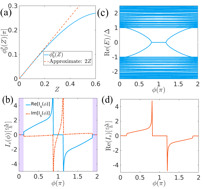
FIG. 3: (a) Josephson-gap phase boundary $\phi_{0}^{p}(Z)$ as a function of $Z$. (b) Complex supercurrent as a function of $\phi$ with $Z=0.2$. The supercurrent diverges at exceptional points. (c) Real energy spectra as a function of $\phi$ from a numerical simulation of the short $p$-wave NHJJ. The Andreev spectra within the superconducting gap host a pair of exceptional points, consistent with analytic results. (d) Real supercurrent derived from the Andreev spectra in (c). It shows sharp peaks and dips at exceptional points. For numerical simulations, we take parameters $m=1$, $\Delta=0.1$, $\mu=0.2$, $h_{z}=0.4,$ $\alpha=0.6$, $V=0.4$, and the junction length $L_{N}=1a$ with $a$ the lattice constant.

For the general solution of the Andreev spectrum, a secular equation is obtained as $(Z^{2}+1)+2iZ\sqrt{\Delta^{2}/E_{B}^{2}-1}=\Delta^{2}\cos^{2}(\frac{\phi}{2})/E_{B}^{2}$ for $p$-wave NHJJs Li2 (a). At $Z=0$, the Andreev spectrum reduces to $E_{B}^{\pm}(\phi)=\pm\Delta\cos(\frac{\phi}{2})$ Kwon et al. (2004). We focus on the regime of small $Z$ as before. In the phase region $\phi\in[\phi_{b}^{p},\phi_{t}^{p}]$, the general solution of the basic equation yields

$$\frac{E_{B}^{\pm}(\phi)}{\Delta}=\frac{\pm\sqrt{\cos^{2}(\frac{\phi}{2})-Z^{2}}-iZ\vartheta\sin(\frac{\phi}{2})}{1-Z^{2}}.$$ (6)

The bottom and top phase boundaries are defined as $\phi_{b}^{p}\equiv 2n\pi+\phi_{0}^{p}(Z)$ and $\phi_{t}^{p}\equiv(2n+1)\pi-\phi_{0}^{p}(Z)$ with $\phi_{0}^{p}(Z)=2\arcsin\left(Z\sqrt{\frac{1-Z^{2}}{1+Z^{2}}}\right)$, and the sign function is given by $\vartheta=\mathrm{sgn}[\sin(\frac{\phi}{2})]$. We plot the Andreev spectrum in $p$-wave NHJJs in Fig. 1(c). The spectrum is also complex, exhibiting Josephson gaps with a gap value of $2\phi_{0}^{p}(Z)$. In the limit $Z\ll 1$, the Josephson-gap phase boundary is $\phi_{0}^{p}(Z)\approx 2Z$ [Fig. 3(a)].

Remarkably, the complex Andreev spectrum hosts a pair of exceptional points (EPs) that are unique to NH systems. The EPs are located at two phases $\text{$\phi_{1}^{e}$}=2\arccos(Z)$ and $\phi_{2}^{e}=2\pi-2\arccos(Z)$ within $\phi\in[0,2\pi]$, as shown in Fig. 1(c) and Fig. 3(c). Their energy takes $E=(0,\frac{-iZ}{\sqrt{1-Z^{2}}})$, with zero real values. Between the two EPs, the real part of spectrum remains at zero. Therefore, the EPs can be controlled by tuning the parameter $Z$. The complex supercurrents carried by the Andreev spectrum are plotted in Fig. 3(b). Notably, the corresponding supercurrents diverge at the EPs. This results in giant supercurrents, which could be functionalized to sensors of the phase difference $\phi$. Note that the real part $\mathrm{Re}[I_{s}(\phi)]$ also vanishes between the two EPs.

Experimental implementation and numerical simulations.—Our proposal of NHJJ with the aforementioned main features is experimentally feasible, considering the advanced fabrication techniques of JJs. The $s$-wave JJs could, for instance, be built based on nanowire JJs Doh et al. (2005); Chang et al. (2015); Hays et al. (2018). The local loss at the junction may stem from the coupling of JJs to the environment with a dissipative lead Zhang et al. (2022b); Liu et al. (2022); Li2 (b). The $p$-wave superconductor can be fabricated by semiconductors with appreciable spin-orbit coupling, such as InAs and InSb, proximitized to $s$-wave superconductors Lutchyn et al. (2010); Oreg et al. (2010); Mourik et al. (2012); Alicea (2012); Aguado (2017); Lutchyn et al. (2018); Frolov et al. (2020). In the following, we provide more convincing evidence from numerical simulations.

The effective NH Hamiltonian for the $p$-wave NHJJ based on semiconductor nanowires is

$$H_{p}=(\frac{-\hbar^{2}\partial_{x}^{2}}{2m}-\mu-i\hbar\alpha\partial_{x}\sigma_{y})\tau_{z}+h_{z}\sigma_{z}+\Delta(x)\tau_{x}+U(x),$$ (7)

where $h_{z}$ is the Zeeman field and $\alpha$ is the Rashba spin-orbit coupling strength. $\Delta(x)$ denotes the proximity effect induced spin-singlet $s$-wave pairing potential. For numerical simulations, we discretize the effective NH Hamiltonian $H_{p}$ on a 1D lattice Li2 (a). In Fig. 3(c), we present the real part of the energy spectra. We find that the Andreev spectrum in the superconducting gap exhibits the main features of the $p$-wave NHJJ as predicted, such as EPs and Josephson gaps Li2 (a). The corresponding supercurrent $\mathrm{Re}[I_{s}(\phi)]$ associated with the Andreev spectrum is shown in Fig. 3(d). We observe that the supercurrent shows sharp peaks and dips at the EPs whereas it vanishes between the two EPs and within Josephson gaps, in good agreement with the previous analytic results.

Conclusion and discussion.—To summarize, we have studied the low-energy spectral features and transport properties of NHJJs. Our minimal model of NHJJs reveals anomalous NH physics emerging in JJs. We have introduced several conceptually new phenomena, such as Josephson gaps, EPs hosted by the complex Andreev spectrum, and divergent supercurrents at EPs, with no counterparts in the Hermitian case.

Our work extends the realm of the Josephson effect to NH physics and inspires potential applications: the NHJJ may function as a supercurrent switch by tuning the phase difference $\phi$ exploiting the presence of Josephson gaps Li2 (a). Moreover, the sensitive response of supercurrents at EPs may be functionalized in sensors Wiersig (2014); Chen et al. (2017); Budich and Bergholtz (2020). The impact of non-Hermiticity on other related phenomena, such as ac Josephson effect, Shapiro steps Tinkham (1996), JJ circuits Devoret and Schoelkopf (2013), and Josephson diode effect Ando et al. (2020), are interesting extensions of our work.

Note added.—Recently, we have noticed a related work on NHJJs Cayao and Sato (2023).

Supplemental material for “Anomalous Andreev Spectrum and Transport in Non-Hermitian Josephson Junctions”

Appendix S1 Non-Hermitian description of the model from the Lindblad formalism

In our setup, the Josephson junction is coupled to the environment. Hence, it is an open quantum system. In the following, we give an argument in which sense this system can be described by the effective non-Hermitian Hamiltonian employed for the description of non-Hermitian Josephson junction (NHJJ) in the main text. The Hamiltonian for the total quantum system is composed of three parts

$$H=H_{S}+H_{E}+H_{I},$$ (S1.1)

where $H_{S}$ is the system Hamiltonian, describing the Josephson junction without coupling to the environment. The degrees of freedom in the environment are described by the Hamiltonian $H_{E}$, and the interaction between system and environment is captured by $H_{I}$. The Hamiltonian of the system can be written in its eigenbasis as $H_{S}=\sum_{n_{s}}(\varepsilon_{n_{s}}-\mu_{s})C_{n_{s}}^{\dagger}C_{n_{s}}$ with eigenenergy $\varepsilon_{n_{s}}$ and eigenstate $|n_{s}\rangle$. Here, $C_{n_{s}}^{\dagger}$ ($C_{n_{s}}$) denotes creation (annihilation) operators of the system. They refer to the occupation of Andreev quasi-bound states. The fermionic environment is described by the Hamiltonian $H_{E}=\sum_{n_{e}}(\varepsilon_{n_{e}}-\mu_{e})C_{n_{e}}^{\dagger}C_{n_{e}}$. We assume that $\mu_{e}<\mu_{s}$, i.e. the chemical potential of the environment is smaller than that of the system. Note that the environment contains the quantum dot as well as the reservoir cf. Fig. S1. The quantum dot works as a monitor to control the tunneling of particles between the system and the reservoir, as we will elaborate on below. The coupling Hamiltonian is given by $H_{I}=\sum_{n_{e},n_{s}}V_{es}C_{n_{e}}^{\dagger}C_{n_{s}}+h.c.$. In general, the interaction term can be decomposed in a way $H_{I}=\sum_{i}S_{i}\otimes E_{i}$ where $S_{i}$ ($E_{i}$) is an operator acting on the system (the environment).

The Lindblad master equation yields the dynamics of the system in presence of dissipation due to the environment. The Lindblad master equation takes (Breuer and Petruccione, 2002; Daley, 2014; Manzano, 2020; Roccati et al., 2022)

$$\frac{d\rho_{S}}{dt} =-i[H_{S},\rho_{S}]+\sum_{m}\gamma(\hat{L}_{m}\rho_{S}\hat{L}_{m}^{\dagger}-\frac{1}{2}\{\hat{L}_{m}^{\dagger}\hat{L}_{m},\rho_{S}\}),$$ (S1.2)

where $\rho_{S}$ is the reduced density matrix of the system, $\hat{L}_{m}$ the Lindblad operator describing the dissipative dynamics (including decoherence and loss processes) occurring at a positive rate $\gamma$ (Daley, 2014). We can further rewrite the Lindblad master equation as

$$\frac{d\rho_{S}}{dt} =-i(H_{\mathrm{eff}}\rho_{S}-\rho_{S}H_{\mathrm{eff}}^{\dagger})+\sum_{m}\gamma\hat{L}_{m}\rho_{S}\hat{L}_{m}^{\dagger},$$

where $H_{\mathrm{eff}}=H_{S}-\frac{i}{2}\sum_{m}\gamma\hat{L}_{m}^{\dagger}\hat{L}_{m}.$ Note that the Lindblad operator $\hat{L}_{m}$ is obtained by tracing out the degrees of freedom from environment on the interaction term (Breuer and Petruccione, 2002). Considering $\mu_{e}<\mu_{s}$, we can assume that the energy modes of the environment coupled to the system are unoccupied (Daley, 2014). In this case, we have $\hat{L}_{m}=C_{m_{s}}.$

The dissipation term $-\frac{i}{2}\sum_{m}\gamma\hat{L}_{m}^{\dagger}\hat{L}_{m}$ describes continuous loss of coherence and energy of the system to the environment. Without the quantum-jump term (Yamamoto et al., 2019; Minganti et al., 2019; Roccati et al., 2022), we obtain the equation of motion

$$\frac{d\text{$\rho_{S}$}}{dt}=-i(H_{\mathrm{eff}}\rho_{S}-\rho_{S}H_{\mathrm{eff}}^{\dagger}),$$ (S1.3)

which is equivalent to work with an effective non-Hermitian Hamiltonian $H_{\mathrm{eff}}=H_{S}-\frac{i}{2}\sum_{m}\gamma\hat{L}_{m}^{\dagger}\hat{L}_{m}$ for describing the system of interest.

The quantum-jump term $\sum_{m}\gamma\hat{L}_{m}\rho_{S}\hat{L}_{m}^{\dagger}$ is related to the abrupt change of quantum trajectories (Minganti et al., 2019; Daley, 2014). The Lindblad operator takes $\hat{L}_{m}=C_{m_{s}}$ in our case. Consider a state $|m_{s}\rangle=|0,\cdots,n_{m},\cdots\rangle$ in the system $H_{s}$. Then the quantum-jump term $\gamma C_{m_{s}}|m_{s}\rangle\langle m_{s}|C_{m_{s}}^{\dagger}$ indicates the annihilation of an excitation in the state $|m_{s}\rangle$. This excitation escapes into the environment. To monitor the quantum-jump process, we assume an auxiliary quantum dot between the junction and the dissipative lead (connected to the reservoir), as shown in Fig. S1. Note that this setup can be experimentally realized (Deng et al., 2016). The quantum dot has a few energy levels. Hence, it is feasible to monitor its occupation e.g. by a nearby quantum point contact. By performing weak measurements and postselection techniques on the quantum dot (Naghiloo et al., 2019), it is possible to only consider those trajectories where no quantum jumps happen during finite time windows. The average over many such quantum trajectories describes the loss physics from the dissipation.

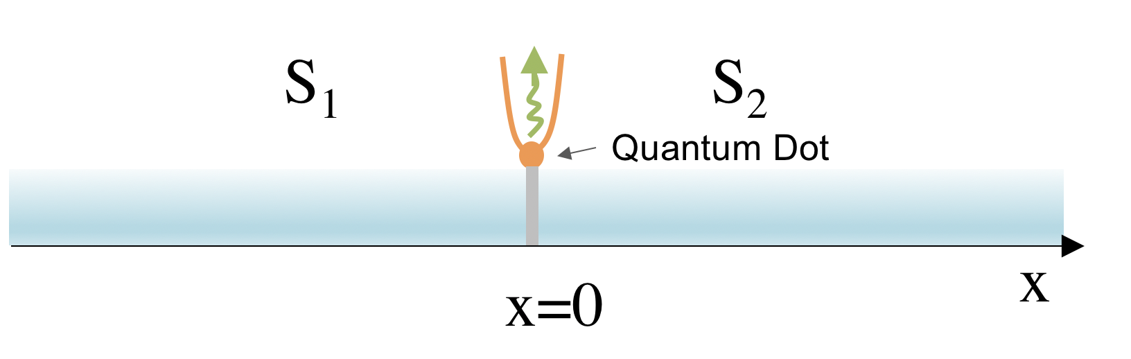
FIG. S1: Sketch of the junction coupled to the environment. There is a quantum dot between the junction and a reservoir.

To capture this loss physics of the system, we can employ a non-Hermitian potential at the junction as

$$U(x)=-iV\delta(x),\ V>0.$$ (S1.4)

This non-Hermitian potential mimics the loss of coherence and particles effectively (see the main text for more details). Therefore, we arrive at an effective non-Hermitian description of the system as

$$H_{\mathrm{NH}}=H_{S}-iV\delta(x).$$ (S1.5)

Appendix S2 Relevant particle-hole symmetry of the model

In this section, we analyze the particle-hole symmetry that is physically relevant from a general form. From a field operator perspective, the particle-hole symmetry (PHS) mixes creation operator $\Psi^{\dagger}$ and annihilation operator $\Psi$ in a way

$$C\Psi_{\alpha}C^{-1}=U_{\alpha\beta}\Psi_{\beta}^{\dagger},\ C\Psi_{\alpha}^{\dagger}C^{-1}=\Psi_{\alpha}U_{\alpha\beta}^{T},$$ (S2.1)

where $U$ represents a unitary matrix and $C$ denotes the PHS operator. A Hamiltonian $H=\Psi_{\alpha}^{\dagger}\mathcal{H}_{\alpha\beta}\Psi_{\beta}$ is particle-hole symmetric if $CHC^{-1}=H$. This implies that the first-quantized Hamiltonian transforms under PHS as

$$C\mathcal{H}^{T}C^{-1}=-\mathcal{H},$$ (S2.2)

where $T$ is the transpose operation. In the Hermitian case, $\mathcal{H}^{T}=\mathcal{H}^{*}$. While in the non-Hermitian case, $\mathcal{H}^{T}\neq\mathcal{H}^{*}$ in general. Thus, the PHS comes in two kinds as (Kawabata et al., 2019a):

$$U\mathcal{H}^{*}U^{-1} =-\mathcal{H},\ \text{$\mathrm{type}$\ I};$$

$$U\mathcal{H}^{T}U^{-1} =-\mathcal{H},\ \mathrm{\text{$\mathrm{type}$\ I}I.}$$ (S2.3)

In the presence of PHS, the excitation energy of $\mathcal{H}$ always comes in pairs. For the two types of PHSs above, the corresponding energy pairs are $E\longleftrightarrow-E^{*}$ for type I PHS and $E\longleftrightarrow-E$ for type II PHS, respectively.

To determine which one of the two types of PHS on $\mathcal{H}$ is physically more relevant, we further consider the constraint of PHS on Green’s function. On the one hand, the effective Hamiltonian $\mathcal{H}$ is directly related with the retarded Green’s function. Note that the poles of the retarded Green’s function yield the eigenvalues of the Hamiltonian, located in the lower half of the complex plane. On the other hand, the physical indication of the retarded Green’s function as a propagator is consistent with causality. The retarded Green’s function is defined in terms of field operators as $G_{\alpha\beta}^{R}(t)=-i\theta(t)\langle[\Psi_{\alpha}(t),\Psi_{\beta}^{\dagger}(0)]\rangle$, where $t$ is the time domain and $\theta(t)$ is a Heaviside step function. Considering PHS on field operators in Green’s function, it leads to

$$G_{\alpha\beta}^{R}(t) =-i\theta(t)\langle[\Psi_{\alpha}(t),\Psi_{\beta}^{\dagger}(0)]\rangle$$

$$=-i\theta(t)\langle C^{-1}C[\Psi_{\alpha}(t),\Psi_{\beta}^{\dagger}(0)]\rangle$$

$$=-i\theta(t)\langle C[\Psi_{\alpha}(t),\Psi_{\beta}^{\dagger}(0)]C^{-1}\rangle$$

$$=-U_{\alpha\gamma}^{*}\langle i\theta(t)[\Psi_{\gamma}^{\dagger}(0),\Psi_{\delta}(-t)]\rangle U_{\delta\beta}^{T}$$

$$=-U_{\alpha\gamma}^{*}G_{\gamma\delta}^{A}(-t)U_{\delta\beta}^{T}.$$ (S2.4)

By Fourier transformation and relating the retarded and advanced Green’s function by $[G_{\alpha\beta}^{R}(E)]^{*}=G_{\alpha\beta}^{A}(E)$, the retarded Green’s function fulfills

$$U^{\dagger}[G^{R}(E)]^{*}U=-G^{R}(-E).$$ (S2.5)

This PHS constraint on retarded Green’s function is consistent with type I PHS acting on $\mathcal{H}$: The eigenvalues of the system (poles of the Green’s function) reside on the same side of the complex plane $\mathrm{Im}[E]\leq 0$. In contrast, from the constraint of type II PHS acting on $\mathcal{H}$, eigenvalues distribute symmetrically in the upper and lower half of the complex plane. This symmetric eigenenergy distribution is not consistent with the eigenvalues obtained from the retarded Green’s function. Thus, it is not compatible with the requirement of causality. Therefore, we argue that type I PHS acting on $\mathcal{H}$ is physically more relevant to describe non-Hermitian systems. This type I PHS is employed in the main text and labeled as $\mathrm{PHS^{\dagger}}$.

Appendix S3 Solution of complex Andreev spectrum in $s$-wave case

In this section, we provide details for the solution of Andreev spectrum in $s$-wave NHJJs. The electron and hole excitations are described by the Bogoliubov-de Gennes (BdG) equation

$$\mathcal{H}_{\mathrm{BdG}}(x)\left(\begin{array}[]{c}u(x)\\ v(x)\end{array}\right) =E\left(\begin{array}[]{c}u(x)\\ v(x)\end{array}\right),$$ (S3.5)

where

$$\mathcal{H}_{\mathrm{BdG}}(x) =\left(\begin{array}[]{cc}-\frac{\hbar^{2}\partial_{x}^{2}}{2m}-\mu+U(x)&\hat{\Delta}(x)\\ \hat{\Delta}^{\dagger}(x)&\frac{\hbar^{2}\partial_{x}^{2}}{2m}+\mu+U(x)\end{array}\right),$$ (S3.8)

and

$$U(x) =-iV\delta(x),\ V>0.$$ (S3.9)

In the eigenstate $(u(x),v(x))^{T}$, the $u(x)$ represents electron-like components and the $v(x)$ represents hole-like components, respectively. $\hbar$ is the Planck constant. The pairing potential is introduced as

$$\Delta(x) =\begin{cases}\Delta,&x<0,\\ \Delta e^{i\phi},&x>0.\end{cases}$$ (S3.10)

In the following, we focus on the bound states within the superconducting gap. The wave function of a bound state decay exponentially for $|x|\rightarrow\infty$. Then, the trial wavefunction can be taken as

$$\psi_{B}(x)=\left(\begin{array}[]{c}u_{B}(x)\\ v_{B}(x)\end{array}\right)=\begin{cases}ae^{ik_{h}x}\left(\begin{array}[]{c}v_{0}\\ u_{0}\end{array}\right)+be^{-ik_{e}x}\left(\begin{array}[]{c}u_{0}\\ v_{0}\end{array}\right),&x<0;\\ ce^{ik_{e}x}\left(\begin{array}[]{c}u_{0}e^{i\phi/2}\\ v_{0}e^{-i\phi/2}\end{array}\right)+de^{-ik_{h}x}\left(\begin{array}[]{c}v_{0}e^{i\phi/2}\\ u_{0}e^{-i\phi/2}\end{array}\right),&x>0,\end{cases}$$ (S3.11)

where the parameters are defined as

$$\hbar k_{e} =\sqrt{2m(\mu+i\sqrt{\Delta^{2}-E^{2}})},\ k_{h}=k_{e}^{*},$$ (S3.12)

and

$$u_{0}^{2} =\frac{1}{2}\left(1+i\frac{\sqrt{\Delta^{2}-E^{2}}}{E}\right),\ v_{0}^{2}=\frac{1}{2}\left(1-i\frac{\sqrt{\Delta^{2}-E^{2}}}{E}\right).$$ (S3.13)

Note that $\frac{u_{0}}{v_{0}}=\frac{E+i\sqrt{\Delta^{2}-E^{2}}}{\Delta}=e^{i\theta}$ with $\theta\equiv\arccos(E/\Delta)$. The bound state has a decay length $\lambda$ given by $\lambda=\frac{\hbar v_{F}}{\Delta}\frac{1}{\sqrt{1-E^{2}/\Delta^{2}}}$. Therefore, the necessary condition for the existence of a bound state is $\mathrm{Re}(\lambda)>0$.

By enforcing continuity of the wave function $\psi_{B}(x=0)$ and the jump condition for the $\psi^{\prime}_{B}(x=0)$, we obtain

$$\psi_{B}(0+) =\psi_{B}(0-),$$

$$\psi^{\prime}_{B}(0+)-\psi^{\prime}_{B}(0-) =-\tau_{z}\frac{2imV}{\hbar^{2}}\psi_{B}(0-).$$ (S3.14)

Here, $\tau_{z}=\mathrm{diag}(1,-1)$ is a Pauli matrix. The secular equation is written as

$$\left(\begin{array}[]{cccc}v_{0}&u_{0}&-u_{0}e^{i\phi/2}&-v_{0}e^{i\phi/2}\\ u_{0}&v_{0}&-v_{0}e^{-i\phi/2}&-u_{0}e^{-i\phi/2}\\ -z_{1}v_{0}&z_{2}u_{0}&u_{0}e^{i\phi/2}&-v_{0}e^{i\phi/2}\\ -z_{2}u_{0}&z_{1}v_{0}&v_{0}e^{-i\phi/2}&-u_{0}e^{-i\phi/2}\end{array}\right)\left(\begin{array}[]{c}a\\ b\\ c\\ d\end{array}\right)=0,$$ (S3.15)

where we have defined

$$Z \equiv\frac{mV}{\hbar^{2}k_{F}},\ z_{1}\equiv 1-2Z,\ z_{2}\equiv 1+2Z.$$ (S3.16)

Note that we have used the approximation $k_{e}\approx k_{h}\approx k_{F}$. The determinant of this coefficient matrix needs to be zero to have nontrivial solutions for the coefficients $a,b,c$, and $d$. After a cumbersome calculation, we arrive at

$$u_{0}^{4}(Z+1)^{2}+v_{0}^{4}(Z-1)^{2}-2u_{0}^{2}v_{0}^{2}(Z^{2}+\cos\phi) =0.$$ (S3.17)

Using Eq. (S3.13), this yields the basic equation to determine Andreev spectrum as

$$(Z^{2}+1)+2Zi\sqrt{\frac{\Delta^{2}}{E^{2}}-1}=\frac{\Delta^{2}}{E^{2}}(Z^{2}+\cos^{2}\frac{\phi}{2}).$$ (S3.18)

Let us first discuss some special limits and present the general solutions later. We mainly focus on the regime $0<Z<1$. Note that there is no bound state when $Z>1$.

• For $\phi=2n\pi$, Eq. (S3.18) becomes

  $$(Z^{2}+1)+2Zi\sqrt{\frac{\Delta^{2}}{E^{2}}-1} =\frac{\Delta^{2}}{E^{2}}(Z^{2}+1).$$ (S3.19)

  Assuming $E\neq 0$, we obtain

  $$+2Zi\sqrt{\frac{\Delta^{2}}{E^{2}}-1} =(\frac{\Delta^{2}}{E^{2}}-1)(Z^{2}+1).$$ (S3.20)

  Defining $x\equiv\frac{\Delta^{2}}{E^{2}}-1$, we get $+2Zi\sqrt{x}=x(Z^{2}+1).$ It gives the trivial solution $E^{2}=\Delta^{2},$ corresponding to $x=0$. If $x\neq 0$, we analyze $-4Z^{2}=x(1+Z^{2})^{2}$ with the solution $E=\pm\Delta\sqrt{\frac{1+Z^{2}}{1-Z^{2}}}.$ This solution does not fulfill the condition of a bound state with $\mathrm{Re}(\lambda)>0.$

• When $\phi=(2n+1)\pi$, we have

  $$(Z^{2}+1)+2Zi\sqrt{\frac{\Delta^{2}}{E^{2}}-1} =\frac{\Delta^{2}}{E^{2}}Z^{2}.$$ (S3.21)

  It yields $E^{2}=\Delta^{2}\frac{Z^{2}}{Z^{2}-1}.$ For $0<Z<1$, the energy is purely imaginary $E=\frac{Z\Delta}{\pm i\sqrt{1-Z^{2}}}.$ If we substitute this result back into the original equation, we obtain $E=\frac{Z\Delta}{+i\sqrt{1-Z^{2}}}$ by fixing the sign convention of $\sqrt{-1}=i$. Therefore, only one branch of the imaginary energy is left.

• We now analyze general solution for arbitrary $\phi$. From the above discussion, we find that the energy $E$ can not vanish. Thus we define $\frac{\Delta^{2}}{E^{2}}\equiv\frac{1}{y}.$ Then, we obtain

  $$(Z^{2}+1)y+2Zi\sqrt{y(1-y)}=Z^{2}+\cos^{2}(\phi/2).$$ (S3.22)

  Defining $A\equiv(Z^{2}+1)$, $B\equiv Z^{2}+\cos^{2}(\phi/2)$, the equation can be simplified as

  $$(A^{2}-4Z^{2})y^{2}+(4Z^{2}-2AB)y+B^{2} =0.$$ (S3.23)

  Solving this equation leads to

  $$y =\frac{Z^{2}[Z^{2}-\sin^{2}(\phi/2)]+\cos^{2}(\phi/2)\pm 2Z\mathrm{sgn}(\cos(\phi/2))\cos(\phi/2)\sqrt{Z^{2}-\sin^{2}(\phi/2)}}{(1-Z^{2})^{2}}$$

  $$=\left(\frac{\mathrm{sgn}(\cos(\phi/2))\cos(\phi/2)\pm Z\sqrt{Z^{2}-\sin^{2}(\phi/2)}}{1-Z^{2}}\right)^{2}.$$ (S3.24)

  This expression can be rewritten as

  $$\frac{E}{\Delta}=\pm\frac{\mathrm{sgn}(\cos(\phi/2))\cos(\phi/2)\pm Z\sqrt{Z^{2}-\sin^{2}(\phi/2)}}{1-Z^{2}}.$$ (S3.25)

  At $Z$=0, it reduces to the Kulik-Omel’yanchuk (KO) limit $E_{B}^{\pm}(\phi)=\pm\Delta\cos(\phi/2)$ (Kulik and Omel’yanchuk, 1975). Considering further the necessary condition for a bound state $\mathrm{Re}(\lambda)>0$, this indicates

  $$\sin^{2}(\phi/2) >\frac{2Z^{2}}{1+Z^{{{}^{2}}}}.$$ (S3.26)

  From this condition, we determine the Josephson-gap phase boundary at

  $$\phi_{0}(Z)=2n\pi\pm 2\arcsin\left(\frac{\sqrt{2}Z}{\sqrt{1+Z^{2}}}\right), \ \ n\in\mathbb{Z}.$$ (S3.27)

  Therefore, the complex Andreev spectrum is given by

  $$\frac{E_{B}^{\pm}(\phi)}{\Delta}=\frac{\pm\zeta\cos[\phi/2]-iZ\sqrt{\sin^{2}(\phi/2)-Z^{2}}}{1-Z^{2}},\ \phi\in[\phi_{b},\phi_{t}],$$ (S3.28)

  where the bottom phase edge is $\phi_{b}\equiv 2n\pi+\phi_{0}(Z)$, the top phase edge is $\phi_{t}\equiv(2n+1)\pi-\phi_{0}(Z)$, and $\zeta=\mathrm{sgn}(\cos(\phi/2))$. If we look at the $\phi\sim 0$ with small $Z,$ $\phi_{0}(Z)\approx 2\sqrt{2}Z$. Then, the energy can be approximately obtained as

  $$E_{B}^{\pm}(\phi_{0})\approx\Delta(\text{$\pm 1$}-iZ^{2}).$$ (S3.29)

Appendix S4 Normal states transport with a non-Hermitian barrier

In this section, we calculate the normal states transport in the presence of a non-Hermitian barrier potential. The Hamiltonian in normal states is

$$H=\frac{\hbar^{2}k^{2}}{2m}-iV\delta(x),V>0.$$ (S4.1)

Then the scattering state at the two sides of barrier can be expressed as

$$\psi(x<0) =e^{ikx}+re^{-ikx},$$

$$\psi(x>0) =te^{ikx},$$ (S4.2)

where $r$ and $t$ are reflection and transmission amplitudes, respectively. Considering the continuity of wave functions and their derivatives, we obtain

$$\psi(x=0^{-}) =\psi(x=0^{+}),$$

$$\psi^{\prime}(x=0^{+}) -\psi^{\prime}(x=0^{-})=-i\frac{2mV}{\hbar^{2}}\psi(0).$$ (S4.3)

This equation leads to

$$1+r =t,\ \ t-1+r=-2Zt.$$ (S4.4)

Thus the transmission and reflection amplitudes are

$$t =\frac{1}{1+Z},\ \ r=\frac{-Z}{1+Z}.$$ (S4.5)

The corresponding transmission and reflection “probabilities” are

$$T =\frac{1}{(1+Z)^{2}},\ \ R=\frac{Z^{2}}{(1+Z)^{2}}.$$ (S4.6)

Note that $T+R=\frac{1+Z^{2}}{(1+Z)^{2}}<1$ when $Z>0$, which corresponds to the loss of quasiparticles to the environment due to the non-Hermitian barrier. In contrast, in the gain case, $T+R\geq 1$ in general. We note that the Andreev spectrum in NHJJs cannot be obtained by using the formula $E^{\pm}=\pm\Delta\sqrt{1-T_{N}\sin^{2}(\phi/2)}$ with this normal transmission $T_{N}$ (Beenakker, 1991).

Appendix S5 Complex supercurrent

In this section, we discuss the supercurrent carried by the complex Andreev spectrum. In Hermitian JJs, the supercurrent is obtained as

$$I_{s}(\phi)=\frac{2e}{\hbar}\frac{d\mathcal{F}(\phi)}{d\phi},$$ (S5.1)

where $\mathcal{F}(\phi)$ is the free energy of the system (Beenakker, 1991). We only consider the zero-temperature limit where the physics is determined by the ground state. This formalism leads to the supercurrent obtained as $I_{s}(\phi)=-\frac{2e}{\hbar}\sum_{n>0}\frac{dE_{n}(\phi)}{d\phi}$ from the Andreev spectrum $E_{n}(\phi)$. In NHJJ, the real part of the complex Andreev spectrum is the physical energy while the imaginary part corresponds to a finite lifetime of each eigenstate. The free energy of NHJJs can be interpreted as the summation of real energy levels, broadened due to imaginary parts up to the Fermi energy (Yamamoto et al., 2019). The free energy can in general be complex in non-Hermitian systems (Zhang et al., 2022a; Li et al., 2021). Following the same reasoning in Hermitian JJs, it is thus a reasonable to generalize the supercurrent as $I_{s}(\phi)=-\frac{2e}{\hbar}\frac{d\mathrm{Re}[E_{B}^{+}(\phi)]}{d\phi}+i\frac{2e}{\hbar}\frac{d\mathrm{Im}[E_{B}^{+}(\phi)]}{d\phi}$, where $E_{B}^{+}(\phi)$ is the complex Andreev spectrum. Substituting the explicit form of the complex Andreev spectrum, we find that the complex supercurrent in the $s$-wave NHJJ is given as

$$I_{s}(\phi)=\frac{\Delta e}{\hbar}\left[\frac{\zeta\sin(\phi/2)}{1-Z^{2}}-i\frac{Z\sin(\phi)}{2(1-Z^{2})\sqrt{\sin^{2}(\phi/2)-Z^{2}}}\right],\ \ \phi\in[\phi_{b},\phi_{t}].$$ (S5.2)

There is no supercurrent in the Josephson gaps.

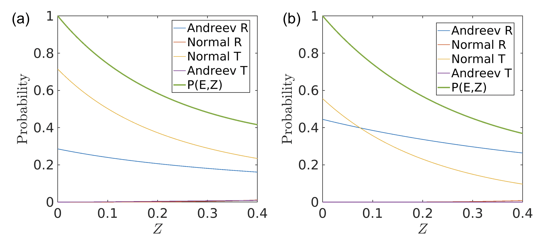
FIG. S2: Scattering probabilities as a function of $Z$. We chose $\phi=\frac{\pi}{2}$ in (a) and $\phi=\pi$ in (b). Other parameters are $\Delta=0.2$ and $E=0.3$.

Appendix S6 Quasiparticle loss due to non-Hermitian barrier scattering

In this section, we obtain the reflection amplitudes (Andreev reflection and the normal reflection) and tunneling amplitudes (crossed Andreev tunneling and the normal tunneling) of quasiparticles after scattering at the non-Hermitian barrier. We show explicitly the loss of quasiparticles from the junction to the environment due to non-Hermitian scatterings. Consider an electron-like quasiparticle that is propagating from the left side of the junction. The wave function can be written as

$$\psi(x)=\left(\begin{array}[]{c}u(x)\\ v(x)\end{array}\right)=\begin{cases}e^{ik_{e}x}\left(\begin{array}[]{c}u_{0}\\ v_{0}\end{array}\right)+A_{h-}e^{ik_{h}x}\left(\begin{array}[]{c}v_{0}\\ u_{0}\end{array}\right)+A_{e-}e^{-ik_{e}x}\left(\begin{array}[]{c}u_{0}\\ v_{0}\end{array}\right),&x<0;\\ A_{e+}e^{ik_{e}x}\left(\begin{array}[]{c}u_{0}e^{i\phi/2}\\ v_{0}e^{-i\phi/2}\end{array}\right)+A_{h+}e^{-ik_{h}x}\left(\begin{array}[]{c}v_{0}e^{i\phi/2}\\ u_{0}e^{-i\phi/2}\end{array}\right),&x>0.\end{cases}$$ (S6.1)

The coefficients are determined by the boundary conditions:

$$\psi(0+) =\psi(0-),$$ (S6.2)

$$\psi^{\prime}(0+)-\psi^{\prime}(0-) =-\tau_{z}\frac{2imV}{\hbar^{2}}\psi(0+).$$ (S6.3)

These boundary conditions can be rewritten as

$$\left(\begin{array}[]{cccc}v_{0}&u_{0}&-u_{0}e^{i\phi/2}&-v_{0}e^{i\phi/2}\\ u_{0}&v_{0}&-v_{0}e^{-i\phi/2}&-u_{0}e^{-i\phi/2}\\ v_{0}&-u_{0}&-z_{1}u_{0}e^{i\phi/2}&z_{2}v_{0}e^{i\phi/2}\\ u_{0}&-v_{0}&-z_{2}v_{0}e^{-i\phi/2}&z_{1}u_{0}e^{-i\phi/2}\end{array}\right)\left(\begin{array}[]{c}A_{h-}\\ A_{e-}\\ A_{e+}\\ A_{h+}\end{array}\right) =\left(\begin{array}[]{c}-u_{0}\\ -v_{0}\\ -u_{0}\\ -v_{0}\end{array}\right).$$ (S6.16)

By solving these linear equations, the four coefficients (Andreev reflection $A_{h-},$ normal reflection $A_{e-}$, normal tunneling $A_{e+}$, crossed Andreev tunneling $A_{h+}$) are obtained as

$$A_{h-} =-\frac{\Delta[E\sin^{2}\frac{\phi}{2}+\Omega(i\sin\frac{\phi}{2}\cos\frac{\phi}{2}-Z)]}{(Z^{2}+1)E^{2}-2Z\Omega E-\Delta^{2}(Z^{2}+\cos^{2}\frac{\phi}{2})},$$ (S6.17)

$$A_{e-} =-\frac{Z\Omega(Z\Omega-E)}{(Z^{2}+1)E^{2}-2Z\Omega E-\Delta^{2}(Z^{2}+\cos^{2}\frac{\phi}{2})},$$ (S6.18)

$$A_{e+} =-\frac{\Omega E(Z\cos\frac{\phi}{2}+i\sin\frac{\phi}{2})-\Omega^{2}(\cos\frac{\phi}{2}+iZ\sin\frac{\phi}{2})}{(Z^{2}+1)E^{2}-2Z\Omega E-\Delta^{2}(Z^{2}+\cos^{2}\frac{\phi}{2})},$$ (S6.19)

$$A_{h+} =\frac{\Delta\Omega Z\cos\frac{\phi}{2}}{(Z^{2}+1)E^{2}-2Z\Omega E-\Delta^{2}(Z^{2}+\cos^{2}\frac{\phi}{2})}.$$ (S6.20)

The parameter $\Omega$ is defined as $\Omega\equiv\sqrt{E^{2}-\Delta^{2}}$. The total scattering probability is defined as

$$P(E,Z)=\sum_{\eta=e/h,s=\pm}|A_{\eta s}|^{2}.$$ (S6.21)

In the Hermitian case, the probability is conserved at $P(E,Z=0)=1$. With nonzero $Z$, we find that the probability $P(E,Z)<1$, which indicates the loss of quasiparticles from the junction to the environment [as shown in Figs. S2(a) and S2(b)]. The probability $P(E,Z)$ decays continuously as increasing the strength of $Z$. Thus, the value of $Z$ measures the magnitude of loss.

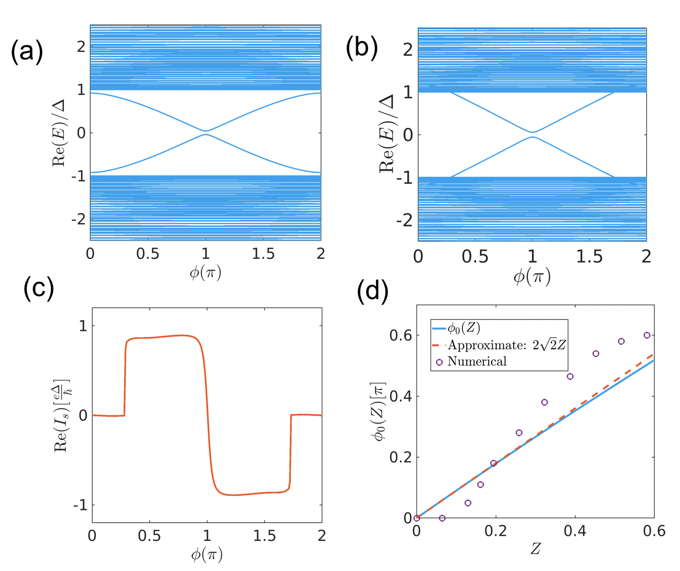
FIG. S3: Tight-binding simulations of the $s$-wave NHJJ with a finite length. (a) Energy spectra as a function of $\phi$ when the loss strength is zero, i.e. $V=0$ and $Z=0$. (b) Real part of energy spectra as a function of $\phi$ when the loss strength is $V=0.4$. (c) Real supercurrent as a function of $\phi$ obtained from corresponding energy spectra in panel (b). (d) Josephson-gap phase boundary $\phi_{0}(Z)$ as a function of $Z$. The circles indicate results extracted from numerical simulations. Other parameters: $m=1,$ $\Delta=0.2$, and $\mu=1.2$.

Appendix S7 Numerical simulations of the $s$-wave non-Hermitian Josephson junction

In this section, we present tight-binding simulations of the $s$-wave NHJJ. The effective Hamiltonian for the $s$-wave NHJJ is

$$H {}_{s}=\left(\begin{array}[]{cc}-\frac{\hbar^{2}\partial_{x}^{2}}{2m}-\mu+U(x)&\Delta(x)\\ \Delta^{*}(x)&\frac{\hbar^{2}\partial_{x}^{2}}{2m}+\mu+U(x)\end{array}\right).$$ (S7.3)

To perform tight-binding calculations, we discretize the Hamiltonian on a one-dimensional (1D) lattice. We take the long-wavelength limit approximation

$$k_{x} \rightarrow\frac{\sin(k_{x}a)}{a},$$

$$k_{x}^{2} \rightarrow 2\frac{1-\cos(k_{x}a)}{a^{2}}.$$ (S7.4)

The lattice constant is set at $a=1$. We divide the system to three parts: the left side and the right side are superconductors of length $L_{s}$, the middle is the normal part of length $L_{N}$. To mimic the loss at the junction, we set $L_{N}=1a$ and an on-site loss potential $-iV$. We take $L_{s}=100a$. The two superconductors have a paring potential $\Delta$ and a phase difference $\phi$.

Figure S3(a) plots energy spectra as a function of $\phi$ when the loss is absent at the junction, i.e. $V=0$ and $Z=0$. A pair of Andreev spectra appear in the superconducting gap, consistent with the result of a bare Josephson junction. Figure S3(b) shows the spectra as a function of $\phi$ when the loss potential is $V=0.4$. It clearly shows a Josephson gap, resembling the analytic results. Figure S3(c) plots the real supercurrent obtained from the Andreev spectra in Fig. S3(b). It is interesting to see that the supercurrent is almost zero within the Josephson gap while it takes nearly a constant otherwise.

To evaluate the phase boundary $\phi_{0}(Z)$, we need the value of $Z$. The parameter $Z$ is given by

$$Z =\frac{mV}{\hbar^{2}k_{F}}=\frac{mV}{\hbar\sqrt{2m\mu}}.$$ (S7.5)

The phase boundary is then obtained as

$$\phi_{0}(Z) =2\arcsin\left(\frac{\sqrt{2}Z}{\sqrt{1+Z^{2}}}\right).$$ (S7.6)

For the parameters used in Fig. S3(b), we find $Z=0.2825$ and $\phi_{0}(Z)=0.252\pi$. The calculated $\phi_{0}$ matches the numerically extracted value $\phi_{0}^{\mathrm{num}}\approx 0.275\pi$. Figure S3(d) presents the phase boundary $\phi_{0}(Z)$ as a function of $Z$. The numerically obtained $\phi_{0}^{\mathrm{num}}(Z)$ qualitatively fits the analytical results, despite some quantitative deviations.

Appendix S8 Solution of complex Andreev spectrum in $p$-wave case

In this section, we present the solution of Andreev spectrum the $p$-wave NHJJ. The BdG equation reads

$$\left(\begin{array}[]{cc}-\frac{\hbar^{2}\partial_{x}^{2}}{2m}-\mu+U(x)&\Delta\hat{k}_{x}/k_{F}\\ (\Delta\hat{k}_{x}/k_{F})^{\dagger}&\frac{\hbar^{2}\partial_{x}^{2}}{2m}+\mu+U(x)\end{array}\right)\left(\begin{array}[]{c}u(x)\\ v(x)\end{array}\right)=E\left(\begin{array}[]{c}u(x)\\ v(x)\end{array}\right).$$ (S8.1)

A At energy $E=0$

In the Hermitian $p$-wave Josephson junction, it is well-known that there exists Majorana zero modes at $\phi=\pi$. To check whether such zero-energy modes are allowed in non-Hermitian $p$-wave junction case, let us first assume $E=0$ in the above equation Eq. (S8.1). In this case, the basis function satisfies the relation $\left(\begin{array}[]{c}u(x)\\ v(x)\end{array}\right)\propto e^{ixk_{e/h}}\left(\begin{array}[]{c}u_{0}\\ v_{0}\end{array}\right)=e^{ixk_{e/h}}\left(\begin{array}[]{c}i\\ 1\end{array}\right)$. It is clear that this wavefunction represents a Majorana zero mode since the Majorana condition $(u,v)^{T}\propto(v^{*},u^{*})^{T}$ can be fulfilled. Next, substituting this wave function into the continuity condition at the junction, this leads to the secular equation

$$u_{0}^{4}(Z-1)^{2}+v_{0}^{4}(Z+1)^{2}+2u_{0}^{2}v_{0}^{2}(Z^{2}-\cos\phi)=0.$$ (S8.2)

This secular equation is valid at $\phi=\pi$ for the assumption $u_{0}=i$ and $v_{0}=1$. Therefore, the Majorana zero modes persist in the $p$-wave NHJJ.

B At energy $E\neq 0$

Following a similar procedure as in the $s$-wave case, we find the secular equation

$$(Z^{2}+1)+2iZ\sqrt{\frac{\Delta^{2}}{E^{2}}-1} =\frac{\Delta^{2}}{E^{2}}\cos^{2}(\phi/2).$$ (S8.3)

Let us first present results for special limits and afterwords the general solutions.

• Josephson phase $\phi=2n\pi$. The above equation becomes

  $$(Z^{2}+1)+2Zi\sqrt{\frac{\Delta^{2}}{E^{2}}-1} =\frac{\Delta^{2}}{E^{2}}.$$ (S8.4)

  Assume $E\neq 0$ to get

  $$+2Zi\sqrt{\frac{\Delta^{2}}{E^{2}}-1} =[\frac{\Delta^{2}}{E^{2}}-(Z^{2}+1)].$$ (S8.5)

  Defining $x\equiv\frac{\Delta^{2}}{E^{2}}-1$, which yields $-2Zi\sqrt{x}=(x-Z^{2})$. The final result is $E=\pm\frac{\Delta}{\sqrt{1-Z^{2}}}$, which does not fulfill the bound state condition $\mathrm{Re}(\lambda)>0$.

• At Josephson phase $\phi=(2n+1)\pi$, the above equation leads to

  $$(Z^{2}+1)+2Zi\sqrt{\frac{\Delta^{2}}{E^{2}}-1} =0.$$ (S8.6)

  When $0<Z<1$, the energy is purely imaginary with $E=\Delta\frac{\pm 2iZ}{1-Z^{2}}.$ Then, if we substitute this solution back to the original equation, we find $E=\Delta\frac{-2iZ}{1-Z^{2}}$ by fixing the sign convention $\sqrt{-1}=i$.

• General Josephson phase $\phi$. We notice that the energy $E$ cannot reach zero now. Thus we define $\frac{\Delta^{2}}{E^{2}}\equiv\frac{1}{y},$ and the equation is simplified to be

  $$(Z^{2}+1)y+2Zi\sqrt{y(1-y)}=\cos^{2}(\phi/2).$$ (S8.7)

  Define $A\equiv(Z^{2}+1)$, $B\equiv\cos^{2}(\phi/2)$ to obtain

  $$(A^{2}-4Z^{2})y^{2}+(4Z^{2}-2AB)y+B^{2} =0.$$ (S8.8)

  Thus, the general solution reads

  $$y =\frac{-2[Z^{2}\sin^{2}(\phi/2)+(Z^{2}-\cos^{2}(\phi/2))]\pm\sqrt{16Z^{2}\sin^{2}(\phi/2)[Z^{2}-\cos^{2}(\phi/2)]}}{2(A^{2}-4Z^{2})}$$

  $$=-\left(\frac{Z\mathrm{sgn}(\sin(\phi/2))\sin(\phi/2)\pm\sqrt{Z^{2}-\cos^{2}(\phi/2)}}{1-Z^{2}}\right)^{2}.$$ (S8.9)

  Finally, we arrive at the result

  $$\frac{E}{\Delta}=\pm i\frac{Z\mathrm{sgn}(\sin(\phi/2))\sin(\phi/2)\pm\sqrt{Z^{2}-\cos^{2}(\phi/2)}}{1-Z^{2}}.$$ (S8.10)

  At $Z=0$, we recover the well-known $p$-wave junction limit with $E=\pm\Delta\cos(\phi/2)$. To determine the Andreev spectrum, we consider the necessary condition for a bound state $\mathrm{Re}(\lambda)>0$, which indicates

  $$\sin^{2}(\phi/2) >\frac{Z^{2}(1-Z^{2})}{1+Z^{{{}^{2}}}}.$$ (S8.11)

  From this condition, we find the Josephson-gap phase boundary at

  $$\phi_{0}^{p}(Z)=2n\pi\pm 2\arcsin\left(Z\sqrt{\frac{1-Z^{2}}{1+Z^{2}}}\right),\ \ n\in\mathbb{Z}.$$ (S8.12)

  Therefore, the Andreev spectrum is given by

  $$\frac{E_{B}^{\pm}(\phi)}{\Delta}=\frac{\pm\sqrt{\cos^{2}(\frac{\phi}{2})-Z^{2}}-i\vartheta Z\sin(\frac{\phi}{2})}{1-Z^{2}},\ \phi\in[\phi_{b}^{p},\phi_{t}^{p}].$$ (S8.13)

  The bottom phase edge is $\phi_{b}^{p}\equiv 2n\pi+\phi_{0}^{p}(Z)$ and the top phase edge is $\phi_{t}^{p}\equiv(2n+1)\pi-\phi_{0}^{p}(Z)$. $\vartheta\equiv\mathrm{sgn}(\sin(\phi/2))$. At $\phi=\pi$, it gives a zero energy mode, consistent with the Majorana zero modes obtained above.

• If we focus on small $Z,$ it gives an approximation relation $\phi_{0}^{p}(Z)\approx 2Z$. At the phase boundary, the energy can be approximated as

  $$E_{B}^{\pm}(\phi_{0}^{p})\approx\Delta(\text{$\pm 1$}-iZ^{2}).$$ (S8.14)

  Interestingly, this value is the same as the one in the $s$-wave case.

• The spectrum shows exceptional points when $\cos^{2}(\frac{\phi}{2})-Z^{2}=0$, which gives $\phi_{e1}=2\arccos(Z)$ and $\phi_{e2}=2\pi-2\arccos(Z)$ in the interested region $[0,2\pi]$. At the exceptional points, two eigenvalue branches coalesce as one. This leads to the unusual behavior of supercurrent associated to the complex Andreev spectrum. The complex supercurrent in the $p$-wave NHJJ is obtained as

  $$I_{s}(\phi)= -\frac{2e}{\hbar}\frac{d\mathrm{Re}[E_{B}^{+}(\phi)]}{d\phi}+i\frac{2e}{\hbar}\frac{d\mathrm{Im}[E_{B}^{+}(\phi)]}{d\phi}$$

  $$= \begin{cases}\frac{\Delta e}{\hbar}&\left(\frac{\sin\phi}{2(1-Z^{2})\sqrt{\cos^{2}(\frac{\phi}{2})-Z^{2}}}-\frac{iZ\vartheta\cos(\frac{\phi}{2})}{1-Z^{2}}\right),\ \ \phi\in[0,\phi_{e1}]\cup[\phi_{e2},2\pi];\\ \frac{\Delta e}{\hbar}&\left(\frac{i\sin\phi}{2(1-Z^{2})\sqrt{Z^{2}-\cos^{2}(\frac{\phi}{2})}}-\frac{iZ\vartheta\cos(\frac{\phi}{2})}{1-Z^{2}}\right),\ \ \phi\in[\phi_{e1},\phi_{e2}].\end{cases}$$

Appendix S9 Numerical simulations of the $p$-wave non-Hermitian Josephson junctions

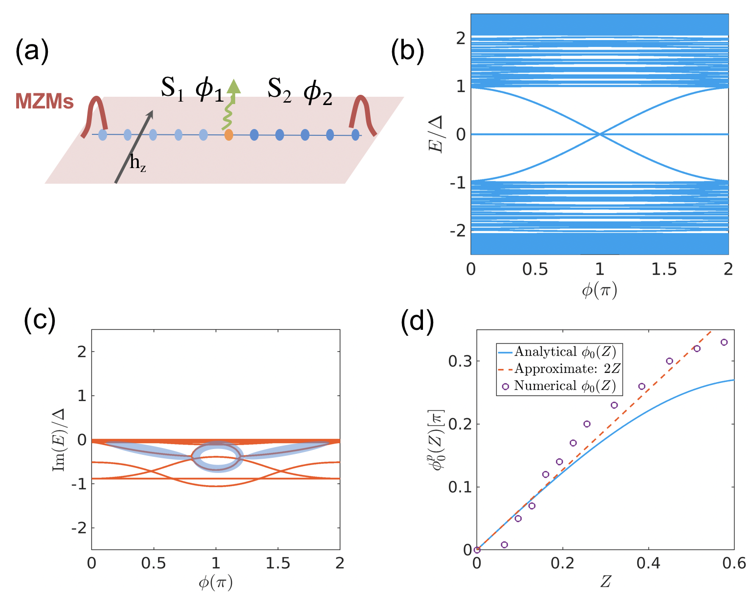
FIG. S4: Tight-binding simulations of the $p$-wave NHJJ with a finite length. (a) The Josephson junction is divided to three regions: the left side and the right side are superconductors of length $L_{s}$, the middle is the normal part of length $L_{N}=1a$ with an on-site loss potential $-iV$. We take $L_{s}=150a$. A Zeeman field with strength $h_{z}$ is applied to the whole region. In the topologically nontrivial phase, there is one Majorana zero mode (MZM) at each ends (red color). (b) Energy spectra as a function of $\phi$ when the loss strength is zero, i.e. $V=0$ and $Z=0$. (c) Imaginary energy spectra corresponding to Fig. 3(c) in the main text. Here $V=0.4$. (d) Josephson-gap phase boundary $\phi_{0}(Z)$ as a function of $Z$. The circles indicate results extracted from numerical simulations. Other parameters: $m=1,$ $\Delta=0.1$, $\mu=0.2$, $h_{z}=0.4$, and $\alpha=0.6$.

In this section, we present tight-binding simulations of the $p$-wave NHJJ. The $p$-wave superconductors can be engineered based on semiconductors by combing the ingredients of strong spin-orbit coupling, Zeeman field, and superconducting proximity effect (Lutchyn et al., 2010; Oreg et al., 2010). The Hamiltonian for the $p$-wave NHJJ based on semiconductor nanowires is

$$H {}_{p}=\left(-\frac{\hbar^{2}\partial_{x}^{2}}{2m}-\mu-i\hbar\alpha\partial_{x}\sigma_{y}\right)\tau_{z}+h_{z}\sigma_{z}+\Delta(x)\tau_{x}+U(x),$$ (S9.1)

where $\alpha$ is the spin-orbit coupling strength, $h_{z}$ is the Zeeman field. $\sigma$ and $\tau$ are Pauli matrices acting on spin and Nambu space, respectively. The topological phase appears under the condition $h_{z}>\sqrt{\Delta^{2}+\mu^{2}}$. There are MZMs at the end of the junction in topologically nontrivial phase [Figs. S4(a) and S4(b)]. To perform tight-binding calculations, we discretize the Hamiltonian $H_{s}$ on a 1D lattice in the same way as in the $s$-wave case above.

Figure S4(b) plots energy spectra when the loss potential is absent at the junction, i.e. $Z=0$. A pair of Andreev spectra cross at $\phi=\pi$. The Majorana zero modes at the two ends (MZMs) show no response to the change of phase difference $\phi$ thus stay at zero energy [Fig. S4(b)]. Note that in Fig. 3(c) of the main text, we neglect the zero-energy states in order to stress the feature of exceptional points. Figure S4(c) presents imaginary energy spectra corresponding to Fig. 3(c) of the main text. The part covered in shadowed region is consistent with the analytical analysis for quasi-bound states, while the additional states come from the continuum.

The numerically obtained $\phi_{0}^{\mathrm{num}}(Z)$ also qualitatively fits the analytical results. To evaluate the phase boundary $\phi_{0}^{p}(Z)$, we need to obtain the value of $Z$. Due to the spin-orbit coupling, the energy bands of semiconductor nanowires take

$$\epsilon_{\pm}(k_{x})=\frac{\hbar^{2}k_{x}^{2}}{2m}-\mu\pm\sqrt{\hbar^{2}\alpha^{2}k_{x}^{2}+h_{z}^{2}}$$ (S9.2)

The Fermi wavevector is approximated as

$$k_{F} =\frac{\sqrt{2}m}{\hbar}\sqrt{(\mu/m+\alpha^{2})+\sqrt{(\mu/m+\alpha^{2})^{2}+(h_{z}^{2}-\mu^{2})^{2}}}.$$ (S9.3)

The the Josephson-gap phase boundary is calculated by using the analytic formula $\phi_{0}^{p}(Z)=2\arcsin\left(Z\sqrt{\frac{1-Z^{2}}{1+Z^{2}}}\right).$ For the parameters used in Fig. 3(c) in the main text, we find $\phi_{0}^{p}=0.154\pi$. The calculated $\phi_{0}^{p}$ matches the numerically extracted value $\phi_{0}^{p,\mathrm{num}}\approx 0.126\pi$. Figure S4(d) shows the phase boundary $\phi_{0}^{p}(Z)$ as a function of $Z$. The numerically obtained $\phi_{0}^{\mathrm{num}}(Z)$ qualitatively fits the analytical results.

References

- Bender (2007) C. M. Bender, “Making sense of non-Hermitian Hamiltonians”, Rep. Prog. Phys. 70, 947 (2007).
- El-Ganainy et al. (2018) R. El-Ganainy, K. G. Makris, M. Khajavikhan, Z. H. Musslimani, S. Rotter, and D. N. Christodoulides, “Non-Hermitian physics and PT symmetry”, Nat. Phys. 14, 11 (2018).
- Ashida et al. (2020) Y. Ashida, Z. Gong, and M. Ueda, “Non-Hermitian physics”, Adv. Phys. 69, 249 (2020).
- Bergholtz et al. (2021) E. J. Bergholtz, J. C. Budich, and F. K. Kunst, “Exceptional topology of non-Hermitian systems”, Rev. Mod. Phys. 93, 015005 (2021).
- Okuma and Sato (2023) N. Okuma and M. Sato, “Non-Hermitian topological phenomena: A review”, Ann. Rev. Condens. Matter Phys. 14, 83 (2023).
- Zyuzin and Zyuzin (2018) A. A. Zyuzin and A. Y. Zyuzin, “Flat band in disorder-driven non-Hermitian Weyl semimetals”, Phys. Rev. B 97, 041203(R) (2018).
- Papaj et al. (2019) M. Papaj, H. Isobe, and L. Fu, “Nodal arc of disordered dirac fermions and non-Hermitian band theory”, Phys. Rev. B 99, 201107(R) (2019).
- Yoshida et al. (2019) T. Yoshida, R. Peters, N. Kawakami, and Y. Hatsugai, “Symmetry-protected exceptional rings in two-dimensional correlated systems with chiral symmetry”, Phys. Rev. B 99, 121101(R) (2019).
- Nagai et al. (2020) Y. Nagai, Y. Qi, H. Isobe, V. Kozii, and L. Fu, “Dmft reveals the non-Hermitian topology and fermi arcs in heavy-fermion systems”, Phys. Rev. Lett. 125, 227204 (2020).
- Makris et al. (2008) K. G. Makris, R. El-Ganainy, D. N. Christodoulides, and Z. H. Musslimani, “Beam dynamics in symmetric optical lattices”, Phys. Rev. Lett. 100, 103904 (2008).
- Guo et al. (2009) A. Guo, G. J. Salamo, D. Duchesne, R. Morandotti, M. Volatier-Ravat, V. Aimez, G. A. Siviloglou, and D. N. Christodoulides, “Observation of -symmetry breaking in complex optical potentials”, Phys. Rev. Lett. 103, 093902 (2009).
- Rotter (2009) I. Rotter, “A non-Hermitian hamilton operator and the physics of open quantum systems”, J. Phys. A: Math. Theor. 42, 153001 (2009).
- Nakagawa et al. (2018) M. Nakagawa, N. Kawakami, and M. Ueda, “Non-Hermitian Kondo effect in ultracold alkaline-earth atoms”, Phys. Rev. Lett. 121, 203001 (2018).
- Xiao et al. (2019) L. Xiao, K. Wang, X. Zhan, Z. Bian, K. Kawabata, M. Ueda, W. Yi, and P. Xue, “Observation of critical phenomena in parity-time-symmetric quantum dynamics”, Phys. Rev. Lett. 123, 230401 (2019).
- Li et al. (2019) J. Li, A. K. Harter, J. Liu, L. de Melo, Y. N. Joglekar, and L. Luo, “Observation of parity-time symmetry breaking transitions in a dissipative floquet system of ultracold atoms”, Nat. Commun. 10, 855 (2019).
- Zhang and Gong (2020) X. Zhang and J. Gong, “Non-Hermitian floquet topological phases: Exceptional points, coalescent edge modes, and the skin effect”, Phys. Rev. B 101, 045415 (2020).
- Dembowski et al. (2001) C. Dembowski, H.-D. Gräf, H. L. Harney, A. Heine, W. D. Heiss, H. Rehfeld, and A. Richter, “Experimental observation of the topological structure of exceptional points”, Phys. Rev. Lett. 86, 787 (2001).
- Berry (2004) M. V. Berry, “Physics of non-Hermitian degeneracies”, Czechoslovak Journal of Physics 54, 1039 (2004).
- Kawabata et al. (2019a) K. Kawabata, T. Bessho, and M. Sato, “Classification of exceptional points and non-Hermitian topological semimetals”, Phys. Rev. Lett. 123, 066405 (2019a).
- Kawabata et al. (2019b) K. Kawabata, K. Shiozaki, M. Ueda, and M. Sato, “Symmetry and topology in non-Hermitian physics”, Phys. Rev. X 9, 041015 (2019b).
- Zhou and Lee (2019) H. Zhou and J. Y. Lee, “Periodic table for topological bands with non-Hermitian symmetries”, Phys. Rev. B 99, 235112 (2019).
- Lee (2016) T. E. Lee, “Anomalous edge state in a non-Hermitian lattice”, Phys. Rev. Lett. 116, 133903 (2016).
- Yao and Wang (2018) S. Yao and Z. Wang, “Edge states and topological invariants of non-Hermitian systems”, Phys. Rev. Lett. 121, 086803 (2018).
- Kunst et al. (2018) F. K. Kunst, E. Edvardsson, J. C. Budich, and E. J. Bergholtz, “Biorthogonal bulk-boundary correspondence in non-Hermitian systems”, Phys. Rev. Lett. 121, 026808 (2018).
- Gong et al. (2018) Z. Gong, Y. Ashida, K. Kawabata, K. Takasan, S. Higashikawa, and M. Ueda, “Topological phases of non-Hermitian systems”, Phys. Rev. X 8, 031079 (2018).
- Zhang et al. (2020) K. Zhang, Z. Yang, and C. Fang, “Correspondence between winding numbers and skin modes in non-Hermitian systems”, Phys. Rev. Lett. 125, 126402 (2020).
- Okuma et al. (2020) N. Okuma, K. Kawabata, K. Shiozaki, and M. Sato, “Topological origin of non-Hermitian skin effects”, Phys. Rev. Lett. 124, 086801 (2020).
- Yao et al. (2018) S. Yao, F. Song, and Z. Wang, “Non-Hermitian Chern bands”, Phys. Rev. Lett. 121, 136802 (2018).
- Leykam et al. (2017) D. Leykam, K. Y. Bliokh, C. Huang, Y. D. Chong, and F. Nori, “Edge modes, degeneracies, and topological numbers in non-Hermitian systems”, Phys. Rev. Lett. 118, 040401 (2017).
- Shen et al. (2018) H. Shen, B. Zhen, and L. Fu, “Topological band theory for non-Hermitian Hamiltonians”, Phys. Rev. Lett. 120, 146402 (2018).
- Yin et al. (2018) C. Yin, H. Jiang, L. Li, R. Lü, and S. Chen, “Geometrical meaning of winding number and its characterization of topological phases in one-dimensional chiral non-Hermitian systems”, Phys. Rev. A 97, 052115 (2018).
- Yokomizo and Murakami (2019) K. Yokomizo and S. Murakami, “Non-bloch band theory of non-Hermitian systems”, Phys. Rev. Lett. 123, 066404 (2019).
- Lee and Thomale (2019) C. H. Lee and R. Thomale, “Anatomy of skin modes and topology in non-Hermitian systems”, Phys. Rev. B 99, 201103(R) (2019).
- Longhi (2019) S. Longhi, “Topological phase transition in non-Hermitian quasicrystals”, Phys. Rev. Lett. 122, 237601 (2019).
- Lee et al. (2019) J. Y. Lee, J. Ahn, H. Zhou, and A. Vishwanath, “Topological correspondence between Hermitian and non-Hermitian systems: Anomalous dynamics”, Phys. Rev. Lett. 123, 206404 (2019).
- Yamamoto et al. (2019) K. Yamamoto, M. Nakagawa, K. Adachi, K. Takasan, M. Ueda, and N. Kawakami, “Theory of non-Hermitian fermionic superfluidity with a complex-valued interaction”, Phys. Rev. Lett. 123, 123601 (2019).
- Borgnia et al. (2020) D. S. Borgnia, A. J. Kruchkov, and R.-J. Slager, “Non-Hermitian boundary modes and topology”, Phys. Rev. Lett. 124, 056802 (2020).
- Budich and Bergholtz (2020) J. C. Budich and E. J. Bergholtz, “Non-Hermitian topological sensors”, Phys. Rev. Lett. 125, 180403 (2020).
- Yamamoto et al. (2021) K. Yamamoto, M. Nakagawa, N. Tsuji, M. Ueda, and N. Kawakami, “Collective excitations and nonequilibrium phase transition in dissipative fermionic superfluids”, Phys. Rev. Lett. 127, 055301 (2021).
- Franca et al. (2022) S. Franca, V. Könye, F. Hassler, J. van den Brink, and C. Fulga, “Non-Hermitian physics without gain or loss: The skin effect of reflected waves”, Phys. Rev. Lett. 129, 086601 (2022).
- Cayao and Black-Schaffer (2022) J. Cayao and A. M. Black-Schaffer, “Exceptional odd-frequency pairing in non-Hermitian superconducting systems”, Phys. Rev. B 105, 094502 (2022).
- Jezequel and Delplace (2023) L. Jezequel and P. Delplace, “Non-Hermitian spectral flows and berry-chern monopoles”, Phys. Rev. Lett. 130, 066601 (2023).
- Qin et al. (2023) F. Qin, R. Shen, and C. H. Lee, “Non-Hermitian squeezed polarons”, Phys. Rev. A 107, L010202 (2023).
- Guo et al. (2023) C.-X. Guo, S. Chen, K. Ding, and H. Hu, “Exceptional non-abelian topology in multiband non-Hermitian systems”, Phys. Rev. Lett. 130, 157201 (2023).
- Cayao and Black-Schaffer (2023) J. Cayao and A. M. Black-Schaffer, “Bulk Bogoliubov fermi arcs in non-Hermitian superconducting systems”, Phys. Rev. B 107, 104515 (2023).
- Sun et al. (2023) J. Sun, C.-A. Li, S. Feng, and H. Guo, “Hybrid higher-order skin-topological effect in hyperbolic lattices”, (2023), arXiv:2305.19810 [cond-mat.mes-hall] .
- Li et al. (2022) C.-A. Li, B. Trauzettel, T. Neupert, and S.-B. Zhang, “Enhancement of second-order non-Hermitian skin effect by magnetic fields”, (2022), arXiv:2212.14691 [cond-mat.mes-hall] .
- Kornich (2023) V. Kornich, “Current-voltage characteristics of the N-I-PT-symmetric non-Hermitian superconductor junction as a probe of non-Hermitian formalisms”, arXiv:2302.14802 (2023).
- Zeuner et al. (2015) J. M. Zeuner, M. C. Rechtsman, Y. Plotnik, Y. Lumer, S. Nolte, M. S. Rudner, M. Segev, and A. Szameit, “Observation of a topological transition in the bulk of a non-Hermitian system”, Phys. Rev. Lett. 115, 040402 (2015).
- Ding et al. (2016) K. Ding, G. Ma, M. Xiao, Z. Q. Zhang, and C. T. Chan, “Emergence, coalescence, and topological properties of multiple exceptional points and their experimental realization”, Phys. Rev. X 6, 021007 (2016).
- Xiao et al. (2020) L. Xiao, T. Deng, K. Wang, G. Zhu, Z. Wang, W. Yi, and P. Xue, “Non-Hermitian bulk–boundary correspondence in quantum dynamics”, Nat. Phys. 16, 761 (2020).
- Ozturk et al. (2021) F. E. Ozturk, T. Lappe, G. Hellmann, J. Schmitt, J. Klaers, F. Vewinger, J. Kroha, and M. Weitz, “Observation of a non-Hermitian phase transition in an optical quantum gas”, Science 372, 88 (2021).
- Liang et al. (2022) Q. Liang, D. Xie, Z. Dong, H. Li, H. Li, B. Gadway, W. Yi, and B. Yan, “Dynamic signatures of non-Hermitian skin effect and topology in ultracold atoms”, Phys. Rev. Lett. 129, 070401 (2022).
- Zhang et al. (2023) Q. Zhang, Y. Li, H. Sun, X. Liu, L. Zhao, X. Feng, X. Fan, and C. Qiu, “Observation of acoustic non-Hermitian bloch braids and associated topological phase transitions”, Phys. Rev. Lett. 130, 017201 (2023).
- Liang et al. (2023) C. Liang, Y. Tang, A.-N. Xu, and Y.-C. Liu, “Observation of exceptional points in thermal atomic ensembles”, Phys. Rev. Lett. 130, 263601 (2023).
- Xu et al. (2023) G. Xu, X. Zhou, Y. Li, Q. Cao, W. Chen, Y. Xiao, L. Yang, and C.-W. Qiu, “Non-Hermitian chiral heat transport”, Phys. Rev. Lett. 130, 266303 (2023).
- Zhu et al. (2016) B. Zhu, R. Lü, and S. Chen, “-symmetry breaking for the scattering problem in a one-dimensional non-Hermitian lattice model”, Phys. Rev. A 93, 032129 (2016).
- Longhi (2017) S. Longhi, “Non-Hermitian bidirectional robust transport”, Phys. Rev. B 95, 014201 (2017).
- Chen and Zhai (2018) Y. Chen and H. Zhai, “Hall conductance of a non-Hermitian Chern insulator”, Phys. Rev. B 98, 245130 (2018).
- Bergholtz and Budich (2019) E. J. Bergholtz and J. C. Budich, “Non-Hermitian Weyl physics in topological insulator ferromagnet junctions”, Phys. Rev. Res. 1, 012003(R) (2019).
- Shobe et al. (2021) K. Shobe, K. Kuramoto, K.-I. Imura, and N. Hatano, “Non-Hermitian Fabry-Pérot resonances in a -symmetric system”, Phys. Rev. Res. 3, 013223 (2021).
- Michen and Budich (2022) B. Michen and J. C. Budich, “Mesoscopic transport signatures of disorder-induced non-Hermitian phases”, Phys. Rev. Res. 4, 023248 (2022).
- Kornich and Trauzettel (2022) V. Kornich and B. Trauzettel, “Andreev bound states in junctions formed by conventional and -symmetric non-Hermitian superconductors”, Phys. Rev. Res. 4, 033201 (2022).
- Sticlet et al. (2022) D. Sticlet, B. Dóra, and C. P. Moca, “Kubo formula for non-Hermitian systems and tachyon optical conductivity”, Phys. Rev. Lett. 128, 016802 (2022).
- Geng et al. (2023) H. Geng, J. Y. Wei, M. H. Zou, L. Sheng, W. Chen, and D. Y. Xing, “Nonreciprocal charge and spin transport induced by non-Hermitian skin effect in mesoscopic heterojunctions”, Phys. Rev. B 107, 035306 (2023).
- Isobe and Nagaosa (2023) H. Isobe and N. Nagaosa, “Anomalous Hall effect from a non-Hermitian viewpoint”, Phys. Rev. B 107, L201116 (2023).
- Likharev (1979) K. K. Likharev, “Superconducting weak links”, Rev. Mod. Phys. 51, 101 (1979).
- Beenakker (1992) C. W. J. Beenakker, “Three “universal” mesoscopic Josephson effects”, in Transport Phenomena in Mesoscopic Systems, edited by H. Fukuyama and T. Ando (Springer Berlin Heidelberg, Berlin, Heidelberg, 1992) pp. 235–253.
- Golubov et al. (2004) A. A. Golubov, M. Y. Kupriyanov, and E. Il’ichev, “The current-phase relation in Josephson junctions”, Rev. Mod. Phys. 76, 411 (2004).
- Tinkham (1996) M. Tinkham, Introduction to Superconductivity (Dover Publications, Inc., Garden City, New York, 1996).
- Furusaki (1999) A. Furusaki, “Josephson current carried by Andreev levels in superconducting quantum point contacts”, Superlattices Microst. 25, 809 (1999).
- Beenakker and van Houten (1991) C. W. J. Beenakker and H. van Houten, “Josephson current through a superconducting quantum point contact shorter than the coherence length”, Phys. Rev. Lett. 66, 3056 (1991).
- Kwon et al. (2004) H.-J. Kwon, K. Sengupta, and V. M. Yakovenko, “Fractional ac Josephson effect in p- and d-wave superconductors”, Eur. Phys. J. B 37, 349 (2004).
- Fu and Kane (2009) L. Fu and C. L. Kane, “Josephson current and noise at a superconductor/quantum-spin-hall-insulator/superconductor junction”, Phys. Rev. B 79, 161408(R) (2009).
- Dolcini et al. (2015) F. Dolcini, M. Houzet, and J. S. Meyer, “Topological Josephson junctions”, Phys. Rev. B 92, 035428 (2015).
- Beenakker et al. (2013) C. W. J. Beenakker, D. I. Pikulin, T. Hyart, H. Schomerus, and J. P. Dahlhaus, “Fermion-parity anomaly of the critical supercurrent in the quantum spin-hall effect”, Phys. Rev. Lett. 110, 017003 (2013).
- Breuer and Petruccione (2002) H. P. Breuer and F. Petruccione, The theory of open quantum systems (Oxford University Press, Great Clarendon Street, 2002).
- Daley (2014) A. J. Daley, “Quantum trajectories and open many-body quantum systems”, Adv. Phys. 63, 77 (2014).
- Minganti et al. (2019) F. Minganti, A. Miranowicz, R. W. Chhajlany, and F. Nori, “Quantum exceptional points of non-Hermitian hamiltonians and liouvillians: The effects of quantum jumps”, Phys. Rev. A 100, 062131 (2019).
- Manzano (2020) D. Manzano, “A short introduction to the lindblad master equation”, AIP Advances 10, 025106 (2020).
- Roccati et al. (2022) F. Roccati, G. M. Palma, F. Ciccarello, and F. Bagarello, “Non-Hermitian physics and master equations”, Open Syst. Inf. Dyn. 29, 2250004 (2022).
- Li2 (a) See Supplemental Material for details of (S1) non-Hermitian description of the model from the Lindblad formalism; (S2) relevant particle-hole symmetry of the model; (S3) solution of complex Andreev spectrum in s-wave case; (S4) the normal states transport with a non-Hermitian potential; (S5) the complex supercurrent; (S6) quasiparticle loss due to non-Hermitian barrier scattering; (S7) numerical simulations of the s-wave non-Hermitian Josephson junctions; (S8) the complex Andreev spectrum in p-wave case, and (S9) numerical simulations of the p-wave non-Hermitian Josephson junctions, which includes Refs. Daley (2014); Minganti et al. (2019); Manzano (2020); Kawabata et al. (2019a); Kulik and Omel’yanchuk (1975); Beenakker (1991); Roccati et al. (2022); Deng et al. (2016); Naghiloo et al. (2019); Breuer and Petruccione (2002); Lutchyn et al. (2010); Oreg et al. (2010); Zhang et al. (2022a); Li et al. (2021); Yamamoto et al. (2019) .
- Nazarov and Blanter (2006) Y. V. Nazarov and Y. M. Blanter, Quantum Transport: Introduction to Nanoscience (Cambridge University Press, 2006).
- Furusaki and Tsukada (1991) A. Furusaki and M. Tsukada, “Dc Josephson effect and andreev reflection”, Solid State Commun. 78, 299 (1991).
- Beenakker (1991) C. W. J. Beenakker, “Universal limit of critical-current fluctuations in mesoscopic Josephson junctions”, Phys. Rev. Lett. 67, 3836 (1991).
- Kulik and Omel’yanchuk (1975) I. O. Kulik and A. N. Omel’yanchuk, “Contribution to the microscopic theory of the Josephson effect in superconducting bridges”, JETP Lett. 21, 96 (1975).
- Note (1) If we assume meV (a typical energy scale of our setup), junction length nm, and Fermi velocity m/s, the parameter can be estimated as . Thus, is of the order of . The value of can in principle be tuned by junction length and loss rate by changing the coupling between JJ and environment.
- Note (2) This competition can be understood by comparing phase difference with the loss parameter .
- Devoret et al. (1990) M. H. Devoret, D. Esteve, H. Grabert, G.-L. Ingold, H. Pothier, and C. Urbina, “Effect of the electromagnetic environment on the Coulomb blockade in ultrasmall tunnel junctions”, Phys. Rev. Lett. 64, 1824 (1990).
- Ingold and Nazarov (1994) G.-L. Ingold and Y. V. Nazarov, in Single charge tunneling: Coulom Blockade Phenomena in Nanostructures, edited by H. Graber and M. H. Devoret (Plenum, Neeew York, 1994) p. 21.
- Hofheinz et al. (2011) M. Hofheinz, F. Portier, Q. Baudouin, P. Joyez, D. Vion, P. Bertet, P. Roche, and D. Esteve, “Bright side of the Coulomb blockade”, Phys. Rev. Lett. 106, 217005 (2011).
- Westig et al. (2017) M. Westig, B. Kubala, O. Parlavecchio, Y. Mukharsky, C. Altimiras, P. Joyez, et al., “Emission of nonclassical radiation by inelastic cooper pair tunneling”, Phys. Rev. Lett. 119, 137001 (2017).
- Grimm et al. (2019) A. Grimm, F. Blanchet, R. Albert, J. Leppäkangas, S. Jebari, D. Hazra, et al., “Bright on-demand source of antibunched microwave photons based on inelastic Cooper pair tunneling”, Phys. Rev. X 9, 021016 (2019).
- Note (3) The lifetime of quasiparticles becomes phase dependent. Thus, the magnitude of imaginary supercurrent indicates the response of quasiparticles loss as changing .
- Note (4) We find that the total scattering probability for an NH barrier, which means parts of quasiparticles escape into the environment from the JJ. More details can be found in the SM Li2 (a).
- Hatano and Nelson (1996) N. Hatano and D. R. Nelson, “Localization transitions in non-Hermitian quantum mechanics”, Phys. Rev. Lett. 77, 570 (1996).
- Zhang et al. (2022a) S.-B. Zhang, M. M. Denner, T. Bzdušek, M. A. Sentef, and T. Neupert, “Symmetry breaking and spectral structure of the interacting hatano-nelson model”, Phys. Rev. B 106, L121102 (2022a).
- Li et al. (2021) Q. Li, J.-J. Liu, and Y.-T. Zhang, “Non-Hermitian Aharonov-Bohm effect in the quantum ring”, Phys. Rev. B 103, 035415 (2021).
- San-Jose et al. (2016) P. San-Jose, J. Cayao, E. Prada, and R. Aguado, “Majorana bound states from exceptional points in non-topological superconductors”, Sci. Rep. 6, 21427 (2016).
- Avila et al. (2019) J. Avila, F. Peñaranda, E. Prada, P. San-Jose, and R. Aguado, “Non-Hermitian topology as a unifying framework for the Andreev versus Majorana states controversy”, Commun. Phys. 2, 133 (2019).
- Doh et al. (2005) Y.-J. Doh, J. A. van Dam, A. L. Roest, E. P. A. M. Bakkers, L. P. Kouwenhoven, and S. De Franceschi, “Tunable supercurrent through semiconductor nanowires”, Science 309, 272 (2005).
- Chang et al. (2015) W. Chang, S. M. Albrecht, T. S. Jespersen, F. Kuemmeth, P. Krogstrup, J. Nygård, and C. M. Marcus, “Hard gap in epitaxial semiconductor–superconductor nanowires”, Nat. Nanotechnol. 10, 232 (2015).
- Hays et al. (2018) M. Hays, G. de Lange, K. Serniak, D. J. van Woerkom, D. Bouman, P. Krogstrup, J. Nygård, A. Geresdi, and M. H. Devoret, “Direct microwave measurement of Andreev-bound-state dynamics in a semiconductor-nanowire Josephson junction”, Phys. Rev. Lett. 121, 047001 (2018).
- Zhang et al. (2022b) S. Zhang, Z. Wang, D. Pan, H. Li, S. Lu, Z. Li, et al., “Suppressing Andreev bound state zero bias peaks using a strongly dissipative lead”, Phys. Rev. Lett. 128, 076803 (2022b).
- Liu et al. (2022) D. Liu, G. Zhang, Z. Cao, H. Zhang, and D. E. Liu, “Universal conductance scaling of Andreev reflections using a dissipative probe”, Phys. Rev. Lett. 128, 076802 (2022).
- Li2 (b) The dissipative lead strongly affects the Andreev spectrum as shown in the experiment .
- Lutchyn et al. (2010) R. M. Lutchyn, J. D. Sau, and S. Das Sarma, “Majorana fermions and a topological phase transition in semiconductor-superconductor heterostructures”, Phys. Rev. Lett. 105, 077001 (2010).
- Oreg et al. (2010) Y. Oreg, G. Refael, and F. von Oppen, “Helical liquids and Majorana bound states in quantum wires”, Phys. Rev. Lett. 105, 177002 (2010).
- Mourik et al. (2012) V. Mourik, K. Zuo, S. M. Frolov, S. R. Plissard, E. P. A. M. Bakkers, and L. P. Kouwenhoven, “Signatures of Majorana fermions in hybrid superconductor-semiconductor nanowire devices”, Science 336, 1003 (2012).
- Alicea (2012) J. Alicea, “New directions in the pursuit of Majorana fermions in solid state systems”, Rep. Prog. Phys. 75, 076501 (2012).
- Aguado (2017) R. Aguado, “Majorana fermions in condensed matter”, Riv. Nuovo Cimento 40, 523 (2017).
- Lutchyn et al. (2018) R. M. Lutchyn, E. P. A. M. Bakkers, L. P. Kouwenhoven, P. Krogstrup, C. M. Marcus, and Y. Oreg, “Majorana zero modes in superconductor–semiconductor heterostructures”, Nat. Rev. Mater. 3, 52 (2018).
- Frolov et al. (2020) S. M. Frolov, M. J. Manfra, and J. D. Sau, “Topological superconductivity in hybrid devices”, Nat. Phys. 16, 718 (2020).
- Wiersig (2014) J. Wiersig, “Enhancing the sensitivity of frequency and energy splitting detection by using exceptional points: Application to microcavity sensors for single-particle detection”, Phys. Rev. Lett. 112, 203901 (2014).
- Chen et al. (2017) W. Chen, Ş. Kaya Özdemir, G. Zhao, J. Wiersig, and L. Yang, “Exceptional points enhance sensing in an optical microcavity”, Nature 548, 192 (2017).
- Devoret and Schoelkopf (2013) M. H. Devoret and R. J. Schoelkopf, “Superconducting circuits for quantum information: An outlook”, Science 339, 1169 (2013).
- Ando et al. (2020) F. Ando, Y. Miyasaka, T. Li, J. Ishizuka, T. Arakawa, Y. Shiota, T. Moriyama, Y. Yanase, and T. Ono, “Observation of superconducting diode effect”, Nature 584, 373 (2020).
- Deng et al. (2016) M. T. Deng, S. Vaitiekenas, E. B. Hansen, J. Danon,M. Leijnse, K. Flensbergg, J. Nygård, P. Krogstrup, and C. M. Marcus, “Majorana bound state in a coupled quantum-dot hybrid-nanowire system”, Science 354, 1557 (2016).
- Naghiloo et al. (2019) M. Naghiloo, M. Abbasi, Y. N. Joglekar, and K. W. Murch, “Quantum state tomography across the exceptional point in a single dissipative qubit”, Nat. Phys. 15, 1232 (2019).
- Cayao and Sato (2023) J. Cayao and M. Sato, “Non-Hermitian phase-biased Josephson junctions”, (2023), arXiv:2307.15472 [cond-mat.supr-con] .