Explicit mathematical epidemiology results on age renewal kernels and $R_{0}$ formulas are often consequences of the rank one property of the next generation matrix

Abstract

A very large class of ODE epidemic models (2) discussed in this paper enjoys the property of admitting also an integral renewal formulation, with respect to an “age of infection kernel” $a(t)$ which has a matrix exponential form (3.2). We observe first that a very short proof of this fact is available when there is only one susceptible compartment, and when its associated “new infections” matrix has rank one. In this case, $a(t)$ normalized to have integral 1, is precisely the probabilistic law which governs the time spent in all the “infectious states associated to the susceptible compartment”, and the normalization is precisely the basic replacement number. The Laplace transform (LT) of $a(t)$ is a generalization of the basic replacement number, and its structure reflects the laws of the times spent in each infectious state. Subsequently, we show that these facts admit extensions to processes with several susceptible classes, provided that all of them have a new infections matrix of rank one. These results reveal that the ODE epidemic models highlighted below have also interesting probabilistic properties.

[a]organization=Departement of Mathematics,University of Pau, city=Pau, postcode=64000, country=France,, addressline= avramf3@gmail.com, [b]organization=Departement of Mathematics,Ibn Tofail University, city=Kenitra, postcode=14000, country=Morocco,, addressline=rim.adenane9@gmail.com

[c]organization=School of Mathematics and Statistics, Shandong University, city= Weihai, postcode=264209, country= China,, addressline= LAMA, Univ Gustave Eiffel, UPEM, Univ Paris Est Creteil, France, dan.goreac@u-pem.fr

[d]organization=Department of mathematics and informatics, Polytechnic University of Bucharest, city=Boucharest, country=Romania, , addressline= andrei.halanay@upb.ro.

1 Introduction

Motivation. Mathematical epidemiology has one fundamental law, which identifies, under certain conditions [38], the threshold parameter $R_{0}$ for the stability of the disease free equilibrium as the Perron-Frobenius eigenvalue of the “next generation matrix” (NGM). Furthermore, explicit $R_{0}$ formulas are also available when the next generation matrix has rank one [6, 1]. It may be argued that this result is not that important, since just computing the eigenvalues of the next generation matrix with any symbolic CAS will reveal $R_{0}$. However, epidemiologic models whose NGM has rank one have a further important property which does not seem to be known well enough: it is the existence of probabilistic renewal kernels – see [15, 1], which may be associated to the times spent by infectious individuals in groups of several infectious states. This property is very important both since it applies to a very large proportion of the models used in applied studies of Covid-19, influenza, ILI (influenza like illnesses), etc., and since it suggests new ways of calibration –see below. Note that this result implies easily that of [6, 1], by integrating the renewal kernel. The lack of awareness for these two fundamental results motivated us to first review them here for the case of one susceptible compartment, and to provide extensions to the case of several susceptible classes. Note especially the formulas (5.8) and (5.7), which seem to be new.

A bird’s eye view of mathematical epidemiology. Mathematical epidemiology may be said to have started with the celebrated paper “A contribution to the mathematical theory of epidemics” [30] on the 1906 plague epidemic in Bombay, which introduced the SIR (susceptible-infected-recovered) model. Bacaer shows that better results can be obtained by adding compartments for rats and fleas [9, (7-11)], whose importance had been overlooked in the first study. In this spirit, each of the three fundamental compartments S,I,R, could be replaced by classes of several compartments, specific to each epidemics, to be revealed by further analyses.

The most fundamental aspect of mathematical epidemiology is the existence of at least two possible fixed states: the boundary “disease free equilibrium” (DFE), corresponding to the elimination of all compartments $\vec{\mathsf{i}}\;$ involving sickness, which may be easily found from the system of non-infectious equations with $\vec{\mathsf{i}}\;=0$, and the “endemic point” which replaces the DFE when elimination of the sickness is impossible (without intervention, such as quarantine, vaccination, etc…). Note this further induces a partition of all the coordinates and the equations into “infectious” (eliminable), and the others, or “non-infectious”. The non-infectious may further be divided into recovered (output compartments) and susceptible (input compartments). The latter are very important; for example, older individuals may be more susceptible than young ones, or viceversa, and therefore differentiating susceptibles into several groups may be crucial.

The most important result of mathematical epidemiology is the “basic reproduction number ” $\mathcal{R}$ threshold theorem concerning the stability of the DFE, already encountered in [30].

There are two flavors of mathematical epidemiology and two corresponding formulas for the basic reproduction number :

1. One, for ODE models, identifies $\mathcal{R}$, under conditions specified in [17, 38, 39], via a three-steps “next generation matrix” (NGM) procedure:

   1. computing a “pre-NGM” matrix which involves only the infectious equations,

   2. substituting into it the coordinates of the DFE, which is obtained using only non-infectious equations, and

   3. computing the spectral radius of the resulting NGM matrix.

2. The “non-Markovian/renewal” approach adds one further crucial aspect to mathematical epidemiology: the change in infectivity as function of age of the infection at the time when transmission took place (which was assumed to be exponentially distributed under the previous approach). This factor enters the model via an “age of infection kernel”, and the basic reproduction number  is computed as the integral of this kernel [17, 18].

The restriction to SIR models with next generation matrix of rank-one renders the connection between the two approaches very elementary and yields powerful explicit formulas – see (5.8) and (5.7) below.

Contents. Section 2 recalls the definition of SIR-PH-FA models. Section 3 computes the age of infection kernel for these models with one susceptible class, when the “new infections” matrix $B$ is of rank one. Section 4 provides examples. Section 5 provides an extension to the case of several susceptible compartments. Section 6 discusses the relation of rank one ODE epidemic models to the generalized linear chain trick (GLCT) formalism. Conclusions and further work are sketched in section 7.

2 SIR-PH-FA epidemic models

The SIR-PH (phase-type) epidemic models [35] are a particular case of the $(A,B)$ Arino-Brauer epidemic models studied in [3, 1], in which there is only one input class $\mathsf{s}$ (and, less importantly, only one output class ${\mathsf{r}}$). One may think of this class of models as of processes in which the class I has been replaced by a transient Markov chain, the time of transition of which models the law (distribution) of the total infectious period. The modeling of infectious laws more general than the exponential is an old concern in epidemiology– see for example  [22, 27] and references therein. Our concern is not only statistical, but also in identifying laws (principles) which hold for large classes of models. Assuming one input class allows decomposing the basic reproduction number  $\mathcal{R}$, defined as the expected number of secondary cases produced by a typical infectious individual during its time of infectiousness– see [24], which serves also as stability threshold of the DFE, as

$$\mathcal{R}=\mathsf{s}_{dfe}\mathcal{R},$$ (2.1)

where $\mathsf{s}_{dfe}$ is the number of susceptibles at the DFE. $\mathcal{R}$ is called basic replacement number (of one susceptible individual). These models include a large number of epidemic models, like for example for COVID and ILI (influenza like illnesses). After further ignoring certain quadratic terms for the varying population model [1], we arrive at a SIR-PH-FA model, defined by:

$$\vec{\mathsf{i}}\;^{\prime}(t) =\vec{\mathsf{i}}\;(t)\left[\mathsf{s}(t)\;B+A-Diag\left[{\mbox{\boldmath$\delta$}}+\Lambda{\mbox{\boldmath$1$}}\right]\right]:=\vec{\mathsf{i}}\;(t)\left[\mathsf{s}(t)B-V\right]$$

$$\mathsf{s}^{\prime}(t) =-\mathsf{s}(t)\vec{\mathsf{i}}\;(t){\mbox{\boldmath$\beta$}}+\Lambda-\left(\Lambda+\gamma_{s}\right)\mathsf{s}(t)+\gamma_{r}{\mathsf{r}}(t),$$

$$\beta =\begin{pmatrix}{\mbox{\boldmath$\beta$}}_{1}\\ \vdots\\ {\mbox{\boldmath$\beta$}}_{n}\end{pmatrix},\quad{\mbox{\boldmath$\beta$}}_{i}=(B{\mbox{\boldmath$1$}})_{i}=\sum_{j}B_{i,j},i=1,...,n$$

$${\mathsf{r}}^{\prime}(t) =\vec{\mathsf{i}}\;(t){\mbox{\boldmath$a$}}+\mathsf{s}(t)\gamma_{s}-(\gamma_{r}+\Lambda){\mathsf{r}}(t),\quad{\mbox{\boldmath$a$}}=(-A){\mbox{\boldmath$1$}}.$$ (2.2)

Here,

1. $\mathsf{s}(t)\in\mathbb{R_{+}}$ represents the set of individuals susceptible to be infected (the beginning state).

2. ${\mathsf{r}}(t)\in\mathbb{R_{+}}$ models recovered individuals (the end state).

3. $\gamma_{r}$ gives the rate at which recovered individuals lose immunity, and $\gamma_{s}$ gives the rate at which individuals are vaccinated (immunized). These two transfers connect directly the beginning and end states (or classes).

4. the row vector $\vec{\mathsf{i}}\;(t)\in\mathbb{R}^{n}$ represents the set of individuals in different disease states.

5. $\Lambda>0$ is the per individual death rate, and it equals also the global birth rate (this is due to the fact that this is a model for proportions).

6. $A$ is a $n\times n$ Markovian sub-generator matrix which describes transfers between the disease classes. Recall that a Markovian sub-generator matrix for which each off-diagonal entry $A_{i,j}$, $i\neq j$, satisfies $A_{i,j}\geq 0$, and such that the row-sums are non-positive, with at least one inequality being strict.

   The fact a Markovian sub-generator appears in our “disease equations” suggests that certain probabilistic concepts intervene in our deterministic model, and this is indeed the case–see below. Note also that typical epidemic models satisfy $A_{i,j}A_{j,i}=0$, $i\neq j$, and so this matrix may be arranged to be triangular.

7. ${\mbox{\boldmath$\delta$}}\in\mathbb{R_{+}}^{n}$ is a column vectors giving the death rates caused by the epidemic in the disease compartments. The matrix $-V$, which combines $A$ and the birth and death rates $\Lambda,{\mbox{\boldmath$\delta$}}$, is also a Markovian sub-generator.

8. $B$ is a $n\times n$ matrix (called sometimes “new infections” matrix). We will denote by $\beta$ the vector containing the sum of the entries in each row of $B$, namely, ${\mbox{\boldmath$\beta$}}=B{\mbox{\boldmath$1$}}$. Its components ${\mbox{\boldmath$\beta$}}_{i}$ represent the total force of infection of the disease class $i$, and $\mathsf{s}(t)\vec{\mathsf{i}}\;(t){\mbox{\boldmath$\beta$}}$ represents the total flux which must leave class $\mathsf{s}$. Finally, each entry $B_{i,j}$, multiplied by $\mathsf{s}$, represents the force of infection from the disease class $i$ onto class $j$, and our essential assumption below will be that $B_{i,j}=\beta_{i}\alpha_{j},$ i.e. that all forces of infection are distributed among the infected classes conforming to the same probability vector $\vec{\alpha}=(\alpha_{1},\alpha_{2},...,\alpha_{n})$.

Remark 1

The matrices $B$ and $-V$, intervene in the formulas related to the next generation matrix approach.

Remark 2

1. Note the factorization of the equation for the diseased compartments $\vec{\mathsf{i}}\;$, which ensures the existence of a fixed point where these compartments vanish, and implies a representation of $\vec{\mathsf{i}}\;$ in terms of $\mathsf{s}$:

   $$\vec{\mathsf{i}}\;(t)=\vec{\mathsf{i}}\;(0)e^{-tV+B\int_{0}^{t}s(\tau)d\tau}=\vec{\mathsf{i}}\;(0)e^{\left[-tId+BV^{-1}\int_{0}^{t}s(\tau)d\tau\right]V}.$$ (2.3)

   In this representation intervenes an essential character of our story, the matrix $BV^{-1},$ which is proportional to the next generation matrix $\mathsf{s}_{dfe}BV^{-1}$. A second representation (3.5) below will allow us to embed our models in the interesting class of distributed delay/renewal models, in the case when $B$ has rank one.

2. When $B={\mbox{\boldmath$\beta$}}\vec{\alpha},$ it holds by the Arino-Brauer formula [6] generalized in [1] that

   $$\mathcal{R}=\lambda_{PF}(\mathsf{s}_{dfe}BV^{-1})=\mathsf{s}_{dfe}\vec{\alpha}V^{-1}{\mbox{\boldmath$\beta$}},$$ (2.4)

   where $\lambda_{PF}$ denotes the Perron-Frobenius eigenvalue (positive eigenvalue of maximum modulus). Note the proof is very simple. The eigenvector must be $v={\mbox{\boldmath$\beta$}}$, and plugging $\beta$ in $\mathsf{s}_{dfe}{\mbox{\boldmath$\beta$}}\vec{\alpha}V^{-1}v=\mathcal{R}v$ yields ${\mbox{\boldmath$\beta$}}(\mathsf{s}_{dfe}\vec{\alpha}V^{-1}{\mbox{\boldmath$\beta$}})=\mathcal{R}{\mbox{\boldmath$\beta$}}$, and the result.

3. We added the FA (first approximation of an exact model for proportions) to the name of these models, following [1], to differentiate them from their version with demography.

3 Associated Markovian semi-groups, age of infection kernels, and an $\mathcal{R}$ formula for SIR-PH-FA models with one susceptible class and $B$ of rank one

We show here that when $B$ has rank one, SIR-PH-FA models have an associated explicit age of infection kernel, which allows in particular obtaining $R_{0}$ via an integral. We may say that rank one SIR-PH-FA epidemic models lie in the intersection of the ODE/Markovian and the non-Markovian/renewal models. Alternatively, they are precisely the renewal models with a matrix-exponential kernel. The equivalence of the two approaches in this simple context is proved concisely below; it may also be read between the lines of the wider scope papers [15, 19].

Our attention to this subject was drawn by formulas on [10, pg. 3] for the “distributed delay/renewal/age of infection kernels” for particular cases of the SIR and SEIR models. These authors assign as an exercise to extend their formulas to other models; it turned out later that determining which models to extend to was part of the exercise. Six years later the exercise was first solved by Champredon-Dushoff-Earn [14] for Erlang-Seir models. We provide below a further extension to the case of SIR-PH-FA models with $B$ of rank one – see also [15, Thm. 2.2], [19] for related results.

Proposition 1

Let $\widetilde{i}(t)=\vec{\mathsf{i}}\;(t){\mbox{\boldmath$\beta$}}$ denote the total force of infection of a SIR-PH-FA model (2) with one susceptible class, without loss of immunity, i.e. $\gamma_{r}=0$, so that $r(t)$ does not affect the rest of the system, and with $B={\mbox{\boldmath$\beta$}}\vec{\alpha}$ of rank one. Then

1. The solutions of the ODE system (2) satisfy also an integro-differential “SI system” of two scalar equations

   $$\begin{cases}\mathsf{s}^{\prime}(t)=\Lambda-\left(\Lambda+\gamma_{s}\right)\mathsf{s}(t)-\mathsf{s}(t)\widetilde{i}(t)\\ \widetilde{i}(t)=\vec{\mathsf{i}}\;(0)e^{-tV}{\mbox{\boldmath$\beta$}}+\int_{0}^{t}s(\tau)\widetilde{i}(\tau)a(t-\tau)d\tau,\end{cases}$$ (3.1)

   where

   $$a(\tau)=\vec{\alpha}e^{-\tau V}{\mbox{\boldmath$\beta$}},$$ (3.2)

   with $-V=A-\left(Diag\left[{\mbox{\boldmath$\delta$}}+\Lambda{\mbox{\boldmath$1$}}\right]\right)$ (it may be checked that this fits the formula on page 3 of [10] for SEIR when $\Lambda=0,\delta=0$).

2. The basic replacement number $\mathcal{R}$ has an integral representation

   $$\mathcal{R}=\int_{0}^{\infty}a(\tau)d\tau=\int_{0}^{\infty}\vec{\alpha}e^{-\tau V}{\mbox{\boldmath$\beta$}}d\tau=\vec{\alpha}\ V^{-1}\;{\mbox{\boldmath$\beta$}}.$$ (3.3)

Proof: 1. The non-homogeneous infectious equations may be transformed into an integral equation by applying the variation of constants formula. The first step is the solution of the homogeneous part. Denoting this by $\Gamma(t)$, it holds that

$$\overset{\rightarrow}{\Gamma}^{\prime}(t) =-\overset{\rightarrow}{\Gamma}(t)V\Longrightarrow\overset{\rightarrow}{\Gamma}(t)=\overset{\rightarrow}{\Gamma}(0)e^{t(-V)}.$$ (3.4)

The variation of constants formula implies then that $\vec{\mathsf{i}}\;(t)$ satisfies  the integral equation:

$$\vec{\mathsf{i}}\;(t)=\vec{\mathsf{i}}\;(0)e^{-tV}+\int_{0}^{t}\mathsf{s}(\tau)\vec{\mathsf{i}}\;(\tau)Be^{-(t-\tau)V}d\tau.$$ (3.5)

Now in the rank one case $B={\mbox{\boldmath$\beta$}}\vec{\alpha}$, and (3.5) becomes

$$\vec{\mathsf{i}}\;(t)=\vec{\mathsf{i}}\;(0)e^{-tV}+\int_{0}^{t}\mathsf{s}(\tau)\vec{\mathsf{i}}\;(\tau){\mbox{\boldmath$\beta$}}\vec{\alpha}e^{-(t-\tau)V}d\tau.$$ (3.6)

Finally, multiplying both sides on the right by $\beta$ yields the result.

2. By the “survival method” , $\mathcal{R}$ may be obtained by integrating $\Gamma(t)$ with $\Gamma(0)=\vec{\alpha}$. A direct proof is also possible by noting that all eigenvalues of the next generation matrix except one are $0$ [6, 1]. $\square$

Remark 3

When $\overset{\rightarrow}{\Gamma}(0)$ is a probability vector, (3.4) has the interesting probabilistic interpretation of the survival probabilities in the various components of the semigroup generated by the Metzler/Markovian sub-generator matrix $-V$ (which inherits this property from the phase-type generator $A$). Practically, $\overset{\rightarrow}{\Gamma}(t)$ will give the expected fractions of individuals who are still in each compartment at time $t$.

Remark 4

We may relate (3.6) to the age of infection equation of the distributed delay/renewal model, by noting that it holds that

$$\vec{\mathsf{i}}\;(t)=\int_{-\infty}^{t}s(\tau)\widetilde{i}(\tau)a(t-\tau)d\tau,$$ (3.7)

provided that $\widetilde{i}(\tau)$ on the interval $(-\infty,0]$ is $\frac{k}{s_{0}}\delta_{0}(\tau),$ where $\delta_{0}(\tau)$ denotes the generalized Dirac function, and that $\vec{\mathsf{i}}\;(0)=k\vec{\alpha}$. This second equation is related to [14, (2.7b),(2.8),(2.9)] and [10, (1)]. Equations like (3.7), called DD (distributed delay) equations appear already in the founding paper [30], which is quite natural. Indeed, if it were known that infections arise precisely $\tau_{0}$ units of time after a contact, then the second equation of the SI model would involve the Dirac kernel $a(\tau)=\delta_{\tau_{0}}(\tau)$. But, since the value of $\tau_{0}$ is never known, it is natural to replace the Dirac kernel by a continuous one.

Remark 5

1. The fact that DD systems can be approximated by ODE systems, by approximating the delay distribution via one of Erlang, and more generally, of matrix-exponential type, has long been exploited in the epidemic literature, under the name of ”linear chain trick” (which has roots in the Erlangization of queueing theory)– see for example  [40, 21, 41, 15, 12, 25, 5, 19] for recent contributions and further references. The opposite direction however, i.e. the solution of the exercise in [10] of identifying the kernels associated to ODE models, seems not to have been resolved in this generality, prior to our paper.

2. Finally, for DD models, normalizing the kernel by its integral $\mathcal{R}$ yields the density of the “intrinsic generating interval” for the age of infection [13, 14, 19]: $g(t)=\frac{a(t)}{\mathcal{R}}=\frac{\vec{\alpha}e^{-\tau V}{\mbox{\boldmath$\beta$}}}{\mathcal{R}}$ –see [14, (2.6)].

4 Examples

4.1 The S$I^{2}$R/SAIR/SEIR-FA epidemic model

We define the S$I^{2}$R/SAIR/SEIR-FA epidemic model [39, 36, 7, 33, 2] by:

Remark 6

1. The classic SEIR model is obtained when $\gamma_{1,r}=0=\delta$. This model maybe viewed as an “Erlangization” of the SIR model, in the sense described by the following definition.

   Definition 1

   a. A (generalized) Erlang row is a matrix row which has one negative element on the main diagonal, followed by its opposite to the right, and in which all the other elements are zero.

   b. A square matrix obtained by adding Erlang rows above a square matrix A, while extending the columns of A by 0’s, will be called an Erlangization of A.

   c. When the extension above involves rows with one negative element on the main diagonal, which is followed to the right by a positive element which is smaller in absolute value, and in which all the other elements are zero, will be called Coxianization. For example, the SI²R model is a Coxianization of the SIR model.

2. Erlangization and Coxianization are particular cases of the generalized linear chain trick – see [25] and the full version of this article. Probabilistically, they amount to preceding a compartment I by another compartment E, such that E may transit either to I or outside the infectious/Markovian classes.

This process has been called in previous papers under several names. Besides SEIR, used usually when $\beta_{1}=0$, but also with $\beta_{1}>0$ – see [39], we have also SITR [42] (when $b=\delta=\gamma_{r}=\gamma_{s}=0$).

The system (4.1) contains nine parameters, three of which $\delta,\gamma_{r}$ and $\gamma_{s}$ do not change much the essence of the problem, and are often omitted. It is an $(A,B)$ Arino-Brauer epidemic models with parameters $\vec{\alpha}=\begin{pmatrix}1&0\end{pmatrix},A=\begin{pmatrix}-\gamma_{1}&\gamma_{1,2}\\ 0&-\gamma_{2}\end{pmatrix},{\mbox{\boldmath$a$}}=(-A){\mbox{\boldmath$1$}}=\begin{pmatrix}\gamma_{1,r}\\ \gamma_{2}\end{pmatrix}$ and

$${\mbox{\boldmath$\beta$}}=\begin{pmatrix}\beta_{1}\\ \beta_{2}\end{pmatrix},\;\mbox{so}\;B=\begin{pmatrix}\beta_{1}&0\\ \beta_{2}&0\end{pmatrix},{\mbox{\boldmath$\delta$}}=\begin{pmatrix}0\\ \delta\end{pmatrix},V=\begin{pmatrix}\gamma_{1}+\Lambda&-\gamma_{1,2}\\ 0&{\gamma_{2}+\Lambda+\delta}\end{pmatrix}.$$

The Laplace transform of the age of infection kernel is:

$$\hat{a}(s) =\vec{\alpha}(sI+V)^{-1}{\mbox{\boldmath$\beta$}}=\beta_{1}\frac{1}{\left(b+\gamma_{1}+s\right)}+\beta_{2}\frac{\gamma_{1,2}}{(b+\gamma_{2}+\delta+s)\left(b+\gamma_{1}+s\right)},$$ (4.2)

and the Arino & al. formula yields $\mathcal{R}=\int_{0}^{\infty}a(\tau)d\tau=\frac{\beta_{1}(b+\gamma_{2}+\delta)+\gamma_{1,2}\beta_{2}}{(b+\gamma_{2}+\delta)\left(b+\gamma_{1}\right)}.$

Remark 7

Probabilistic interpretations of the matrix exponential. (4.2) confirms that the coefficients of $\beta_{i}$ in the delay kernel $a(t)$ are the components $\vec{\Gamma}_{1}(t),\vec{\Gamma}_{2}(t)$ of the semigroup starting from the first state $\vec{\Gamma}(t)=(1,0)e^{-tV}$, namely an exponential with parameter $b+\gamma_{1}$, corresponding to surviving in the exposed/asymptomatic period, and a hypoexponential survival function corresponding to surviving in the infectious state.

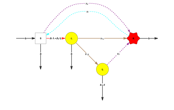
Figure 1: Chart flow of the SAIR model (4.1). The red edge corresponds to the entrance of susceptibles into the disease classes, the brown edges are the rate of the transition matrix V, and the cyan dashed lines correspond to the rate of loss of immunity. The remaining black lines correspond to the inputs and outputs of the birth and natural death rates, respectively, which are equal in this case.

4.2 A generealized SLAIR epidemic model

The SLAIR epidemic model [42, 8, 4] is defined by:

This is an $(A,B)$ Arino-Brauer epidemic models with parameters

The Laplace transform of the age of infection kernel is:

and the Arino & al. formula yields $\mathcal{R}=\frac{\beta_{3}\gamma_{\text{1,2}}\gamma_{\text{2,3}}+b\beta_{2}\gamma_{\text{1,2}}+\beta_{2}\gamma_{3}\gamma_{\text{1,2}}+b\beta_{3}\gamma_{\text{1,3}}+\beta_{3}\gamma_{2}\gamma_{\text{1,3}}}{\left(b+\gamma_{1}\right)\left(b+\gamma_{2}\right)\left(b+\gamma_{3}\right)}.$

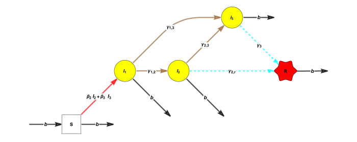
Figure 2: Chart flow of the SLAIR model (4.3).

5 Extension to several susceptible compartments and time-dependent inputs

We show here that SIR-PH epidemic models with two or more susceptible compartments may also satisfy  renewal type integro differential equations.

Consider the ODE model with $n$ infectious classes $\vec{\mathsf{i}}\;=(i_{1},i_{2},...,i_{n}),$ $2$ susceptible classes with arrivals $\Lambda_{1}(t),\Lambda_{1}(t)$, and total arrivals $\Lambda(t)=\Lambda_{1}(t)+\Lambda_{2}(t),$ defined by:

$$\mathsf{s}_{1}^{\prime}(t) =\Lambda_{1}(t)+\gamma_{r,1}{\mathsf{r}}(t)-\mathsf{s}_{1}(t)\left[\vec{\mathsf{i}}\;(t){{\mbox{\boldmath$\beta$}}_{1}}+\Lambda(t)+\gamma_{s}\right],\;\;{\mbox{\boldmath$\beta$}}_{1}=B_{1}{\mbox{\boldmath$1$}},$$

$$\mathsf{s}_{2}^{\prime}(t) =\Lambda_{2}(t)+\gamma_{r,2}{\mathsf{r}}(t)-\mathsf{s}_{2}(t)\left[\vec{\mathsf{i}}\;(t){{\mbox{\boldmath$\beta$}}_{2}}+\Lambda(t)+\gamma_{s}\right],\;\;{\mbox{\boldmath$\beta$}}_{2}=B_{2}{\mbox{\boldmath$1$}},$$

$$\vec{\mathsf{i}}\;^{\prime}(t) =\vec{\mathsf{i}}\;(t)\left[\mathsf{s}_{1}(t)\;B_{1}+\mathsf{s}_{2}(t)\;B_{2}+A-Diag\left(\Lambda(t){\mbox{\boldmath$1$}}+{\mbox{\boldmath$\delta$}}\right)\right]:=\vec{\mathsf{i}}\;(t)\;F(t)-\vec{\mathsf{i}}\;(t)V,$$

$${\mathsf{r}}^{\prime}(t) =\vec{\mathsf{i}}\;(t){\mbox{\boldmath$a$}}+(\mathsf{s}_{1}(t)+\mathsf{s}_{2}(t))\gamma_{s}-(\gamma_{r}+\Lambda(t)){\mathsf{r}}(t),\;{\mbox{\boldmath$a$}}=(-A){\mbox{\boldmath$1$}},$$ (5.1)

where we put $F(t)=\sum_{i}\mathsf{s}_{i}(t)B_{i},{\mbox{\boldmath$\delta$}}=\begin{pmatrix}\delta_{1}\\ \delta_{2}\\ \vdots\end{pmatrix},\gamma_{r}=\gamma_{r,1}+\gamma_{r,2}$. Note that

$$N(t)=\mathsf{s}_{1}(t)+\mathsf{s}_{2}(t)+{\mathsf{r}}(t)+\vec{\mathsf{i}}\;(t){\mbox{\boldmath$1$}}\text{ satisfies }\;N^{\prime}(t)=\Lambda(t)(1-N(t))-\vec{\mathsf{i}}\;(t){\mbox{\boldmath$\delta$}}.$$

Assume further that $B_{i}={\mbox{\boldmath$\beta$}}_{i}\vec{\alpha}_{i},i=1,2$, note the factorization

$$F(t)={{\mbox{\boldmath$\beta$}}}\begin{pmatrix}\mathsf{s}_{1}(t)&0\\ 0&\mathsf{s}_{2}(t)\end{pmatrix}{\vec{\alpha}},\text{ where }{\mbox{\boldmath$\beta$}}=\begin{pmatrix}{\mbox{\boldmath$\beta$}}_{1},&{\mbox{\boldmath$\beta$}}_{2}\end{pmatrix},{\vec{\alpha}}=\begin{pmatrix}\vec{\alpha}_{1}\\ \vec{\alpha}_{2}\end{pmatrix}$$ (5.2)

are $n\times 2$ and $2\times n$ matrices, respectively.

The variation of constants formula applied to (5) implies that $\vec{\mathsf{i}}\;(t)$ satisfies  the integral equation:

$$\vec{\mathsf{i}}\;(t) = \vec{\mathsf{i}}\;(0)e^{-tV}+\int_{0}^{t}\vec{\mathsf{i}}\;(\tau)F(\tau)e^{-(t-\tau)V}d\tau=\vec{\mathsf{i}}\;(0)e^{-tV}+\int_{0}^{t}\vec{\mathsf{i}}\;(t-\tau)F(t-\tau)e^{-\tau V}d\tau$$

$$: = \vec{\mathsf{i}}\;(0)e^{-tV}+\int_{0}^{t}\vec{\mathsf{i}}\;(t-\tau)\widetilde{K}(t,\tau)d\tau,\quad\widetilde{K}(t,\tau):=F(t-\tau)e^{-\tau V}.$$ (5.3)

We will call $\widetilde{K}(t,\tau)$ implicit kernel, to emphasize the fact that it depends still on the unknown $\mathsf{s}_{i}(t)$.

When $B_{i}={\mbox{\boldmath$\beta$}}_{i}\vec{\alpha}_{i},i=1,2$, putting $\widetilde{i}_{i}(t)=\vec{\mathsf{i}}\;(t){\mbox{\boldmath$\beta$}}_{i},i=1,2$ (5) becomes

$$\vec{\mathsf{i}}\;(t)=\vec{\mathsf{i}}\;(0)e^{-tV}+\int_{0}^{t}\left[\sum_{i=1}^{2}\mathsf{s}_{i}(\tau)\widetilde{i}_{i}(\tau)\vec{\alpha}_{i}e^{-(t-\tau)V}\right]d\tau.$$ (5.4)

Multiplying further by ${\mbox{\boldmath$\beta$}}_{k},k=1,2$ and putting

$$a_{i,j}(t)=\vec{\alpha}_{i}e^{-tV}{\mbox{\boldmath$\beta$}}_{j},i,j=1,2,$$ (5.5)

yields a system of two equations for $\widetilde{i}_{k}(t)=\vec{\mathsf{i}}\;(t){\mbox{\boldmath$\beta$}}_{k},k=1,2$:

$$\begin{cases}\widetilde{i}_{1}(t)=\vec{\mathsf{i}}\;(0)e^{-tV}{\mbox{\boldmath$\beta$}}_{1}+\int_{0}^{t}\left[\mathsf{s}_{1}(\tau)\widetilde{i}_{1}(\tau)a_{1,1}(t-\tau)+\mathsf{s}_{2}(\tau)\widetilde{i}_{2}(\tau)a_{2,1}(t-\tau)\right]d\tau\\ \widetilde{i}_{2}(t)=\vec{\mathsf{i}}\;(0)e^{-tV}{\mbox{\boldmath$\beta$}}_{2}+\int_{0}^{t}\left[\mathsf{s}_{1}(\tau)\widetilde{i}_{1}(\tau)a_{1,2}(t-\tau)+\mathsf{s}_{2}(\tau)\widetilde{i}_{2}(\tau)a_{2,2}(t-\tau)\right]d\tau\end{cases}$$ (5.6)

We may conclude that proposition 1 extends as follows:

Proposition 2

Consider a SIR-PH-FA model (5) with two susceptible classes with $B_{i}={\mbox{\boldmath$\beta$}}_{i}\vec{\alpha}_{i},i=1,2$, with constant input inflows $\Lambda_{1},\Lambda_{2}$, and which satisfies the conditions of [38]. Then, it holds that :

1. The solutions of (5) satisfy also an integro-differential system

   $$\begin{cases}\mathsf{s}_{1}^{\prime}(t)=\Lambda_{1}+\gamma_{r,1}{\mathsf{r}}(t)-\mathsf{s}_{1}(t)\left[\vec{\mathsf{i}}\;(t){{\mbox{\boldmath$\beta$}}_{1}}+\Lambda+\gamma_{s}\right],\;\;{\mbox{\boldmath$\beta$}}_{1}=B_{1}{\mbox{\boldmath$1$}},\\ \mathsf{s}_{2}^{\prime}(t)=\Lambda_{2}+\gamma_{r,2}{\mathsf{r}}(t)-\mathsf{s}_{2}(t)\left[\vec{\mathsf{i}}\;(t){{\mbox{\boldmath$\beta$}}_{2}}+\Lambda+\gamma_{s}\right],\;\;{\mbox{\boldmath$\beta$}}_{2}=B_{2}{\mbox{\boldmath$1$}},\\ {\mathsf{r}}^{\prime}(t)=\vec{\mathsf{i}}\;(t){\mbox{\boldmath$a$}}+(\mathsf{s}_{1}(t)+\mathsf{s}_{2}(t))\gamma_{s}-(\gamma_{r}+\Lambda){\mathsf{r}}(t),\;{\mbox{\boldmath$a$}}=(-A){\mbox{\boldmath$1$}}\\ \widetilde{i}(t)=\vec{\mathsf{i}}\;(0)e^{-tV}{\mbox{\boldmath$\beta$}}+\int_{0}^{t}\widetilde{i}(\tau)Diag(\mathsf{s}(\tau))a(t-\tau)d\tau,\end{cases}$$ (5.7)

   where $a(\tau)=\begin{pmatrix}\mathsf{s}_{i}(\tau)a_{i,j}(\tau)\end{pmatrix}_{i,j=1,2},\mathsf{s}(\tau)=(\mathsf{s}_{1}(\tau),\mathsf{s}_{2}(\tau))$.

2. There is a unique DFE, given by

   $$\mathsf{s}_{dfe}^{i}=\frac{\Lambda+\gamma_{s}}{\Lambda_{i}+\gamma_{r,i}\mathsf{r}_{dfe}},i=1,2,\;\mathsf{r}_{dfe}=\frac{\gamma_{s}}{\Lambda+\gamma_{r}+\gamma_{s}}=\frac{\gamma_{s}}{\sum_{i}\Lambda_{i}+\sum_{i}\gamma_{r,i}+\gamma_{s}}.$$

3. If ${\mbox{\boldmath$\beta$}}_{1},{\mbox{\boldmath$\beta$}}_{2}$ are independent, then the basic reproduction number  $\mathcal{R}$ is the Perron-Frobenius eigenvalue of the two by two matrix

   $$M_{D}:=\begin{pmatrix}\mathsf{s}_{dfe}^{1}\vec{\alpha}_{1}V^{-1}{\mbox{\boldmath$\beta$}}_{1}&\mathsf{s}_{dfe}^{1}\vec{\alpha}_{1}V^{-1}{\mbox{\boldmath$\beta$}}_{2}\\ \mathsf{s}_{dfe}^{2}\vec{\alpha}_{2}V^{-1}{\mbox{\boldmath$\beta$}}_{1}&\mathsf{s}_{dfe}^{2}\vec{\alpha}_{2}V^{-1}{\mbox{\boldmath$\beta$}}_{2}\end{pmatrix}={\vec{\alpha}}\begin{pmatrix}\mathsf{s}_{dfe}^{1}&0\\ 0&\mathsf{s}_{dfe}^{2}\end{pmatrix}V^{-1}{\mbox{\boldmath$\beta$}},$$ (5.8)

   with an obvious generalization to the case of several compartments.

Proof. 1. This holds by (5.6).

2. This is an elementary computation.

3. One may check that the conditions of [38] hold, and thus the stability of the unique DFE is determined by the spectral radius of the next generation matrix

$$(\mathsf{s}_{dfe}^{1}B_{1}+\mathsf{s}_{dfe}^{2}B_{2})V^{-1},$$

which coincides with the Perron-Frobenius eigenvalue.

Note first that when $B_{i}={\mbox{\boldmath$\beta$}}_{i}\vec{\alpha}_{i}$, then $B:=\mathsf{s}_{dfe}^{1}B_{1}+\mathsf{s}_{dfe}^{2}B_{2}$ has rank $2$, and so does the next generation matrix. Therefore, all its eigenvalues except at most two are $0$.

We show now that both the remaining eigenvalues satisfy also a $2\times 2$ eigenvalue problem, extending the proof sketched in Remark 1.2. We note first that the corresponding eigenvectors to the right of the next generation matrixmust be of the form $v=\kappa_{1}{\mbox{\boldmath$\beta$}}_{1}+\kappa_{2}{\mbox{\boldmath$\beta$}}_{2}$. Plugging now this form yields the homogeneous $n\times 2$ system for $\kappa_{i},i=1,2$:

$$\left[(\mathsf{s}_{dfe}^{1}{\mbox{\boldmath$\beta$}}_{1}\vec{\alpha}_{1}+\mathsf{s}_{dfe}^{2}{\mbox{\boldmath$\beta$}}_{2}\vec{\alpha}_{2})V^{-1}-\mathcal{R}I_{n}\right]\begin{pmatrix}{\mbox{\boldmath$\beta$}}_{1},&{\mbox{\boldmath$\beta$}}_{2}\end{pmatrix}\begin{pmatrix}\kappa_{1}\\ \kappa_{2}\end{pmatrix}=0$$

For non-zero solutions, the $n\times 2$ matrix multiplying $\begin{pmatrix}\kappa_{1}\\ \kappa_{2}\end{pmatrix}$ must have rank one.

Putting further $a_{ij}=\vec{\alpha}_{i}V^{-1}{\mbox{\boldmath$\beta$}}_{j}$, we may rewrite the matrix as

$$\begin{pmatrix}\mathsf{s}_{dfe}^{1}{\mbox{\boldmath$\beta$}}_{1}a_{11}+\mathsf{s}_{dfe}^{2}{\mbox{\boldmath$\beta$}}_{2}a_{21},&\mathsf{s}_{dfe}^{1}{\mbox{\boldmath$\beta$}}_{1}a_{12}+\mathsf{s}_{dfe}^{2}{\mbox{\boldmath$\beta$}}_{2}a_{22}\end{pmatrix}-\mathcal{R}\begin{pmatrix}{\mbox{\boldmath$\beta$}}_{1},&{\mbox{\boldmath$\beta$}}_{2}\end{pmatrix}=\begin{pmatrix}{\mbox{\boldmath$\beta$}}_{1},&{\mbox{\boldmath$\beta$}}_{2}\end{pmatrix}(M_{D}-\mathcal{R}I_{2}).$$

Now if $deterministic(M_{D}-\mathcal{R}I_{2})=0,$ i.e. if (5.8) holds, then this matrix has rank one, and if ${\mbox{\boldmath$\beta$}}_{1},{\mbox{\boldmath$\beta$}}_{2}$ are independent, then this condition is also necessary. Finally, we note that when the matrix $M_{D}$ has two positive eigenvalues, then $\mathcal{R}$ will be their maximum.

One example where this formula applies is the vector–host model in [38, Sec. 4.5].

Remark 8

The formula for the basic reproduction number , in examples with two susceptible classes, involves sometimes square roots – see for example [28, 26], [31, (7,9)], [37, Sec. 6.1]. Other times it is $\max[\mathcal{R}_{1},\mathcal{R}_{2}]$ where $\mathcal{R}_{1},\mathcal{R}_{2}$ involve only one susceptible class, and are obtained by the rank one basic reproduction number  formulas (this is sometimes referred to as competitive exclusion). Our formula (5.8) suggests that the difference between the two situations comes from the reduced next generation matrix (or the Diekmann kernel) being triangular or not.

6 Extending rank one ODE epidemic models via the generalized linear chain trick (GLCT) formalism, and the associated renewal models

The rank one models discussed in this paper arise often via the so-called generalized linear chain trick [25]. For example, the SIR-PH with one susceptible class arises by splitting the I individuals into several subcompartments, with in-between transitions governed by an $(\vec{\alpha},A)$ phase type distribution. This model may be viewed also as a SIR renewal model, for which the time spent in the infectious class is of type $(\vec{\alpha},A)$. The GLCT formalism (GLCTF) is best explained via the example of the SEIR model.

6.1 The SEIR-PH GLCT model

We recall here a probabilistically interpretable SEIR-PH model, due to [25, 27], and compute its Diekmann kernel and basic replacement number $\mathcal{R}$. Recall the classic SEIR model

$$\frac{dS}{dt}= \;-\beta\,S\,I$$ (6.1a)

$$\frac{dE}{dt}= \;\beta\,S\,I-r_{E}\,E$$ (6.1b)

$$\frac{dI}{dt}= \;r_{E}\,E-r_{I}\,I$$ (6.1c)

$$\frac{dR}{dt}= \;r_{I}\,I,$$ (6.1d)

where we have assumed no demography, which renders the computation of the semigroup simpler. Assume now the latent period distribution is phase-type with parameters $\vec{\alpha}_{\mathbf{E}}$ and $\mathbf{A_{E}}$, and the infectious period distribution is also phase-type, but with parameters $\vec{\alpha}_{\mathbf{I}}$ and $\mathbf{A_{I}}$. Let $\;\vec{\mathsf{x}}=[E_{1},\ldots]$ and $\;\vec{\mathsf{y}}=[I_{1},\ldots]$ be the row vectors of the fraction of individuals in each of the exposed and infectious sub-states, respectively, and put $E=\sum E_{j}$ and $I=\sum I_{i}$. An associated ODE model, which may be obtained either by introducing auxiliary unknowns $\;\vec{\mathsf{x}},\;\vec{\mathsf{y}}$ into the SEIR model (6.1), or directly by GLCTF, is:

$$\frac{dS}{dt}= \;-\beta\,S\,I$$ (6.2a)

$$\frac{d\;\vec{\mathsf{x}}}{dt}= \;\beta\,S\,I\,\vec{\alpha}_{\mathbf{E}}+\;\vec{\mathsf{x}}{\mathbf{A_{E}}}$$ (6.2b)

$$\frac{d\;\vec{\mathsf{y}}}{dt}= \;\underbrace{\big{(}\;\vec{\mathsf{x}}{\mbox{\boldmath$a$}}_{E}\big{)}}_{\text{destruction scalars}}\cdotp\vec{\alpha}_{\mathbf{I}}+\;\vec{\mathsf{y}}{\mathbf{A_{I}}},\quad{\mbox{\boldmath$a$}}_{E}=-{\mathbf{A_{E}}\mathbf{1}}$$ (6.2c)

$$\frac{dR}{dt}= \;\overbrace{\;\vec{\mathsf{y}}{\mbox{\boldmath$a$}}_{I}},\quad{\mbox{\boldmath$a$}}_{I}={-\mathbf{A_{I}}\mathbf{1}}.$$ (6.2d)

Remark 9

The first fact to note in (6.2) is that the scalar transfer rates $r_{E},r_{I}$ have been replaced by transfer matrices $\mathbf{A_{E}},\mathbf{A_{I}}$, in their “origine equations” (6.1b), (6.1c), respectively. The second key fact to note that in the “destination equations” (6.1c), (6.1d), $r_{E},r_{I}$ have been replaced by the product of “destruction scalars” (ending with ${\mbox{\boldmath$a$}}_{E},{\mbox{\boldmath$a$}}_{I}$) by “rebirth vectors” ($\vec{\alpha}_{\mathbf{I}}$ for the first, and $1$ for the second). This is the matrix expression of the usual balance between out-flows and in-flows, which takes into account the different dimensionality of the origines and destinations.

This is an $(A,B)$ Arino-Brauer epidemic model with one susceptible class and parameters

$$-V=\mathbf{A}=\begin{pmatrix}{\mathbf{A_{E}}}&{\mbox{\boldmath$a$}}_{E}\vec{\alpha}_{I}\\ 0&{\mathbf{A_{I}}}\end{pmatrix},\vec{\alpha}=\begin{pmatrix}\vec{\alpha}_{E}&0\end{pmatrix},{\mbox{\boldmath$\beta$}}=\begin{pmatrix}0\\ \beta{\mbox{\boldmath$1$}}\end{pmatrix}.$$

Remark 10

Researchers familiar with the interpretations of ${\mbox{\boldmath$a$}}_{E}$ and $\vec{\alpha}_{I}$ as death rates in E states and birth rates in I states will note the intuition behind the formulas, as well as the fact that by grouping together E, I, in an I class, the SEIR-PH may be viewed also as a SIR-PH. Finally, note that the generalization to heterogeneous infectivity rates ${\mbox{\boldmath$\beta$}}=\begin{pmatrix}\beta_{1}\\ \beta_{2}\\ \vdots\end{pmatrix}$ is immediate.

By the [6] formula, the basic reproduction number  is

$$\mathcal{R}=\begin{pmatrix}\vec{\alpha}_{E}&0\end{pmatrix}\begin{pmatrix}-{\mathbf{A_{E}}}^{-1}&{\mathbf{A_{E}}}^{-1}{\mbox{\boldmath$a$}}_{E}\vec{\alpha}_{I}{\mathbf{A_{I}}}^{-1}\\ 0&-{\mathbf{A_{I}}}^{-1}\end{pmatrix}\begin{pmatrix}0\\ \beta{\mbox{\boldmath$1$}}\end{pmatrix}=-\beta\vec{\alpha}_{I}{\mathbf{A_{I}}}^{-1}{\mbox{\boldmath$1$}}=\beta{\mathbb{E}}[\tau_{E}+\tau_{I}],$$ (6.3)

where $\tau_{E},\tau_{I}$ denote the distributions of the total times spent in exposed and infectious classes, respectively, and ${\mathbb{E}}$ denotes mathematical expectation. The semigroup is quasi-explicit, given by

$$e^{t\mathbf{A}}=\begin{pmatrix}e^{t\mathbf{A_{E}}}&ILT\left[(sId-\mathbf{A_{E}})^{-1}{\mbox{\boldmath$a$}}_{E}\vec{\alpha}_{I}(sId-\mathbf{A_{I}})^{-1}\right]\\ \mathbf{0}&e^{t\mathbf{A_{I}}},\end{pmatrix}$$ (6.4)

where $ILT$ denotes inverse Laplace transform.

Example 1

For example, suppose

$$\mathbf{A_{E}}=\begin{pmatrix}-\eta_{E}&\eta_{E}\\ 0&-r_{E}\end{pmatrix},{\mbox{\boldmath$a$}}_{E}=\begin{pmatrix}0\\ r_{E}\end{pmatrix},\mathbf{A_{I}}=\begin{pmatrix}-\eta_{I}&\eta_{I}\\ 0&-r_{I}\end{pmatrix},{\mbox{\boldmath$a$}}_{I}=\begin{pmatrix}0\\ r_{I}\end{pmatrix},\vec{\alpha}_{I}=(1,0).$$

Then, $\mathbf{A}=\begin{pmatrix}-\eta_{E}&\eta_{E}&0&0\\ 0&-r_{E}&r_{E}&0\\ 0&0&-\eta_{I}&\eta_{I}\\ 0&0&0&-r_{I}\end{pmatrix}$, reflecting the Erlangization of the $E$ and $I$ classes.

The semigroup $e^{tA}$ is explicit, for example the LT transform in its NE corner is

$$\frac{1}{\eta_{i}+s}\frac{r_{e}}{r_{e}+s}\left(\begin{array}[]{cc}\frac{\eta_{e}}{\eta_{e}+s}&\frac{\eta_{e}}{\eta_{e}+s}\frac{\eta_{i}}{r_{i}+s}\\ 1&\frac{\eta_{i}}{r_{i}+s}\\ \end{array}\right).$$

6.2 A seven compartments epidemic model of Covid-19 inspired by [32, 20]

The following seven compartments epidemic model of Covid-19 includes besides the omnipresent $\mathsf{s},i$, also additional super-spreaders, hospitalized, recovery and fatality classes denoted by $p,h,r,f$, respectively. It is given by:

$$\begin{cases}\mathsf{s}^{\prime}(t)=-\beta_{i}\mathsf{s}(t)i(t)-\beta_{h}\mathsf{s}(t)\mathsf{h}(t)-\beta_{p}\mathsf{s}(t)\mathsf{p}(t)\\ \begin{pmatrix}\;\mathsf{e}^{\prime}(t)&i^{\prime}(t)&\mathsf{p}^{\prime}(t)&\mathsf{h}^{\prime}(t)\end{pmatrix}=\begin{pmatrix}\;\mathsf{e}(t)&i(t)&\mathsf{p}(t)&\mathsf{h}(t)\end{pmatrix}\Biggl{[}\mathsf{s}(t)\left(\begin{array}[]{cccc}0&0&0&0\\ \beta_{i}&0&0&0\\ \beta_{p}&0&0&0\\ \beta_{h}&0&0&0\\ \end{array}\right)+\\ \left(\begin{array}[]{cccc}-\gamma_{e}-e_{r}&e_{i}&e_{p}&0\\ 0&-i_{h}-i_{r}-\delta_{i}&0&i_{h}\\ 0&0&-p_{h}-i_{r}-\delta_{p}&p_{h}\\ 0&0&0&-\gamma_{h}-\delta_{h}\\ \end{array}\right)\Biggr{]}\\ \begin{pmatrix}r^{\prime}(t)&\mathsf{f}^{\prime}(t)\end{pmatrix}=\begin{pmatrix}\;\mathsf{e}(t)&i(t)&\mathsf{p}(t)&\mathsf{h}(t)\end{pmatrix}\left(\begin{array}[]{cccc}e_{r}&i_{r}&p_{r}&\gamma_{h}\\ 0&\delta_{i}&\delta_{p}&\delta_{h}\\ \end{array}\right)^{t}\end{cases}.$$ (6.5)

Remark 11

We have removed from the original model a class called asymptomatic, because that class was not allowed to produce new infections [32, Fig 1], as it should have under the usual definition of asymptomatics – see for example [7], and also did not allow recovery, which was probably a typo.

This is an $(A,B)$ Arino-Brauer epidemic models with parameters

$$V=\left(\begin{array}[]{cccc}\gamma_{e}&-e_{i}&-e_{p}&0\\ 0&i_{h}+i_{r}+\delta_{i}&0&-i_{h}\\ 0&0&\mathsf{p}_{h}+p_{r}+\delta_{p}&-\mathsf{p}_{h}\\ 0&0&0&\gamma_{h}+\delta_{h}\\ \end{array}\right),\vec{\alpha}=\begin{pmatrix}1&0&0&0\end{pmatrix},{\mbox{\boldmath$\beta$}}=\begin{pmatrix}0\\ \beta_{i}\\ \beta_{p}\\ \beta_{h}\end{pmatrix}.$$

The Arino & al. formula yields $\mathcal{R}=e_{p}\frac{\beta_{h}p_{h}+\beta_{p}\left(\delta_{h}+\gamma_{h}\right)}{\gamma_{e}\left(p_{h}+\delta_{p}+p_{r}\right)\left(\delta_{h}+\gamma_{h}\right)}+e_{i}\frac{\beta_{h}i_{h}+\beta_{i}\left(\delta_{h}+\gamma_{h}\right)}{\gamma_{e}\left(i_{h}+\delta_{i}+i_{r}\right)\left(\delta_{h}+\gamma_{h}\right)}.$

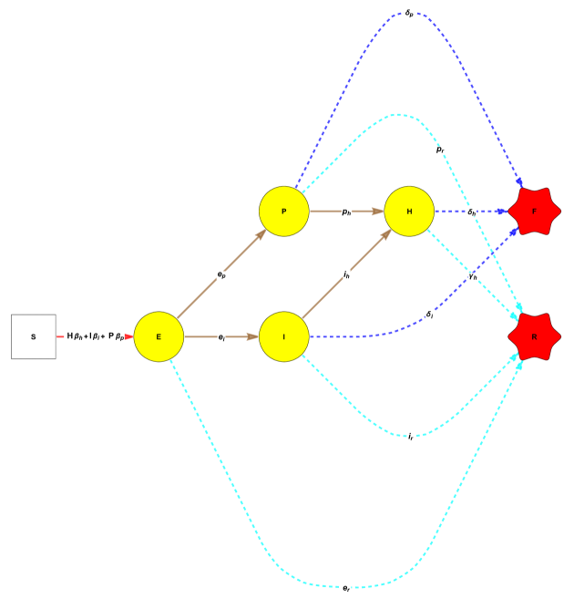
Figure 3: Chart flow of the Covid-19 model (6.5).

Remark 12

[20] argue that the transitions from $i$ and $\mathsf{p}$ to $\mathsf{h}$ should be modeled via DD equations, obtained by replacing $i,\mathsf{p}$ by convolutions with exponential densities, and obtain associated ODE’s with two extra unknowns. We note here that their system loses the conservation of mass of the [32] system, but that this may be maintained by applying GLCT, as follows.

1. Start by introducing new auxiliary variables

   $$\widetilde{i}(t)=\int_{0}^{t}\eta_{i}e^{-\eta_{i}(t-\tau)}\,i(\tau)d\tau,\;\widetilde{\mathsf{p}}(t)=\int_{0}^{t}\eta_{p}e^{-\eta_{p}(t-\tau)}\,\mathsf{p}(\tau)d\tau,$$

   (note that these converge to $e(t),p(t)$ when $\eta_{p},\eta_{i}\to\infty$).

2. Replace $i,\mathsf{p}$ in the equation for $\mathsf{h}$ by $\widetilde{i},\widetilde{\mathsf{p}}$.

3. Add the differential equations $\frac{d\widetilde{i}}{dt}=\;\eta_{i}\,i-\eta_{i}\,\widetilde{i}\;\;\frac{d\widetilde{\mathsf{p}}}{dt}=\eta_{p}\,\mathsf{p}-\eta_{p}\,\widetilde{\mathsf{p}}$ to the ODE system.

Finally, we arrive, for the 6 extended disease equations, to:

$$\begin{cases}\;\mathsf{e}^{\prime}(t)=\beta_{i}\mathsf{s}(t)i(t)+\beta_{p}\mathsf{s}(t)\mathsf{p}(t)+\beta_{h}\mathsf{s}(t)\mathsf{h}(t)-\gamma_{e}\;\mathsf{e}(t),\\ i^{\prime}(t)=e_{i}\;\mathsf{e}(t)-(i_{h}+i_{r}+\delta_{i})i(t),\\ \widetilde{i}^{\prime}(t)=\eta_{i}i(t)-\eta_{i}\widetilde{i}(t),\\ \mathsf{p}^{\prime}(t)=e_{p}\;\mathsf{e}(t)-(p_{h}+p_{r}+\delta_{p})\mathsf{p}(t),\\ \widetilde{\mathsf{p}}^{\prime}(t)=\eta_{p}\mathsf{p}(t)-\eta_{p}\widetilde{\mathsf{p}}(t),\\ \mathsf{h}^{\prime}(t)=i_{h}\widetilde{i}(t)+p_{h}\widetilde{\mathsf{p}}(t)-(\gamma_{h}+\delta_{h})\mathsf{h}(t)\end{cases}$$

This is an $(A,B)$ Arino-Brauer epidemic models with disease variables

$\begin{pmatrix}\;\mathsf{e}(t)&i(t)&\widetilde{i}(t)&\mathsf{p}(t)&\widetilde{\mathsf{p}}(t)&\mathsf{h}(t)\end{pmatrix}$ and parameters $\vec{\alpha}=\begin{pmatrix}1&0&0&0&0&0\end{pmatrix},$

$$V=\left(\begin{array}[]{cccccc}\gamma_{e}&-e_{i}&0&-e_{p}&0&0\\ 0&i_{h}+i_{r}+\delta_{i}&-\eta_{i}&0&0&0\\ 0&0&\eta_{i}&0&0&-i_{h}\\ 0&0&0&p_{h}+p_{r}+\delta_{p}&-\eta_{p}&0\\ 0&0&0&0&\eta_{p}&-p_{h}\\ 0&0&0&0&0&\gamma_{h}+\delta_{h}\\ \end{array}\right),{\mbox{\boldmath$\beta$}}=\begin{pmatrix}0\\ \beta_{i}\\ 0\\ \beta_{p}\\ 0\\ \beta_{h}\end{pmatrix}.$$

We must assume that $i_{h}<\eta_{i},p_{h}<\eta_{p}$, so that $A$ is a sub-generator. It follows than by the formula of Arino $\&$ al. that:

$$\mathcal{R}=e_{p}\frac{\beta_{h}p_{h}+\beta_{p}\left(\delta_{h}+\gamma_{h}\right)}{\gamma_{e}\left(\delta_{h}+\gamma_{h}\right)\left(\delta_{p}+p_{h}+p_{r}\right)}+e_{i}\frac{\beta_{h}i_{h}+\beta_{i}\left(\delta_{h}+\gamma_{h}\right)}{\gamma_{e}\left(\delta_{h}+\gamma_{h}\right)\left(\delta_{i}+i_{h}+i_{r}\right)},$$

which is precisely the same $\mathcal{R}$ as before the extension.

Remark 13

There does not seem to be much practical estimation work of phase-type distributions fitting real epidemic data – see though [25, 29].

In the following subsection we present one example for which we plan to undertake such work in the future.

7 Conclusions and further work

Solving the exercise of [10] revealed that the $(A,B)$ Arino-Brauer epidemic models with $B$ of rank one have the remarkable property of having a natural associated “age of infection kernel” which implies a very simple formula for $\mathcal{R}$. This continues to be true for models with several susceptible classes, and is of considerable interest for epidemic models structured by the age of the individuals.

We prove now that (5.7) has a stationary point with $\widetilde{i}\neq(0,0)$ iff $\mathcal{R}$ defined in (5.8) is bigger than $1$, that this stationary point is locally stable.

This proof reveals also that $\mathcal{R}$ may also be obtained as the spectral radius of the integral of the matrix kernel $K(\tau)=Diag(\mathsf{s}_{dfe})a(\tau),\mathsf{s}_{dfe}=(\mathsf{s}_{dfe}^{1},\mathsf{s}_{dfe}^{2})$. We will call the matrix $K(\tau)$ above Diekmann matrix kernel, in reference to [15, (5.9)], where such matrices seem to have appeared for the first time. Note that in our situation $K(\tau)$ is explicit.

Another question worth further research is whether an age of infection kernel may be associated to $(A,B)$ Arino-Brauer epidemic models with one susceptible class, but with a matrix $B$ of rank bigger than $1$.

The results of this paper suggest an interesting alternative to the classical statistical approaches to mathematical epidemiology, which usually start by postulating an epidemiologic model, and then estimate its parameters. The alternative consists in accepting that the model is not fully known. and estimate instead an age of infection kernel. Subsequently, a good matrix exponential approximation of the kernel will translate directly into an epidemiologic model, to be confronted with the currently accepted ones.

Aknowledgements. We thank Tyler Cassidy, Odo Diekmann, and James Watmough for useful remarks.

References

- AAB+ [23] Florin Avram, Rim Adenane, Lasko Basnarkov, Gianluca Bianchin, Dan Goreac, and Andrei Halanay, An age of infection kernel, an formula and further results for arino-brauer matrix epidemic models with varying population, waning immunity, and disease and vaccination fatalities, Mathematics (2023).
- AAH [22] Florin Avram, Rim Adenane, and Andrei Halanay, New results and open questions for sir-ph epidemic models with linear birth rate, waning immunity, vaccination, and disease and vaccination fatalities, Symmetry 14 (2022), no. 5, 995.
- AAK [21] Florin Avram, Rim Adenane, and David I Ketcheson, A review of matrix SIR arino epidemic models, Mathematics 9 (2021), no. 13, 1513.
- [4] Rim Adenane, Florin Avram, and Rafael Villanueva, Calibrating the sir, seir, and slair epidemic models to influenza data, with mathematica, Mathematica Journa submitted.
- ABG [20] Alessia Andò, Dimitri Breda, and Giulia Gava, How fast is the linear chain trick? a rigorous analysis in the context of behavioral epidemiology., Mathematical Biosciences and Engineering 17 (2020), no. 5, 5059–5085.
- ABvdD+ [07] Julien Arino, Fred Brauer, Pauline van den Driessche, James Watmough, and Jianhong Wu, A final size relation for epidemic models, Mathematical Biosciences & Engineering 4 (2007), no. 2, 159.
- AKK+ [20] Santosh Ansumali, Shaurya Kaushal, Aloke Kumar, Meher K Prakash, and M Vidyasagar, Modelling a pandemic with asymptomatic patients, impact of lockdown and herd immunity, with applications to sars-cov-2, Annual reviews in control (2020).
- AP [20] Julien Arino and Stéphanie Portet, A simple model for covid-19, Infectious Disease Modelling 5 (2020), 309–315.
- Bac [12] Nicolas Bacaër, The model of Kermack and McKendrick for the plague epidemic in Bombay and the type reproduction number with seasonality, Journal of mathematical biology 64 (2012), no. 3, 403–422.
- BDDG+ [12] Dimitri Breda, Odo Diekmann, WF De Graaf, A Pugliese, and R Vermiglio, On the formulation of epidemic models (an appraisal of kermack and mckendrick), Journal of biological dynamics 6 (2012), no. sup2, 103–117.
- Bra [05] Fred Brauer, The kermack–mckendrick epidemic model revisited, Mathematical biosciences 198 (2005), no. 2, 119–131.
- CCH [18] Tyler Cassidy, Morgan Craig, and Antony R Humphries, A recipe for state dependent distributed delay differential equations, arXiv preprint arXiv:1811.05930 (2018).
- CD [15] David Champredon and Jonathan Dushoff, Intrinsic and realized generation intervals in infectious-disease transmission, Proceedings of the Royal Society B: Biological Sciences 282 (2015), no. 1821, 20152026.
- CDE [18] David Champredon, Jonathan Dushoff, and David JD Earn, Equivalence of the erlang-distributed seir epidemic model and the renewal equation, SIAM Journal on Applied Mathematics 78 (2018), no. 6, 3258–3278.
- DGM [18] Odo Diekmann, Mats Gyllenberg, and JAJ Metz, Finite dimensional state representation of linear and nonlinear delay systems, Journal of Dynamics and Differential Equations 30 (2018), no. 4, 1439–1467.
- DHB [13] O. Diekmann, H. Heesterbeek, and T. Britton, Mathematical Tools for Understanding Infectious Disease Dynamics, Princeton Univ. Press, 2013.
- DHM [90] Odo Diekmann, Johan Andre Peter Heesterbeek, and Johan AJ Metz, On the definition and the computation of the basic reproduction ratio r0 in models for infectious diseases in heterogeneous populations, Journal of mathematical biology 28 (1990), no. 4, 365–382.
- DHR [10] Odo Diekmann, JAP Heesterbeek, and Michael G Roberts, The construction of next-generation matrices for compartmental epidemic models, Journal of the royal society interface 7 (2010), no. 47, 873–885.
- DI [22] Odo Diekmann and Hisashi Inaba, A systematic procedure for incorporating separable static heterogeneity into compartmental epidemic models, arXiv preprint arXiv:2207.02339 (2022).
- DSZ [22] Alexander Domoshnitsky, Alexander Sitkin, and Lea Zuckerman, Mathematical modeling of covid-19 transmission in the form of system of integro-differential equations, Mathematics 10 (2022), no. 23, 4500.
- [21] Zhilan Feng, Final and peak epidemic sizes for SEIR models with quarantine and isolation, Mathematical Biosciences & Engineering 4 (2007), no. 4, 675.
- [22] Zhilan Feng, Final and peak epidemic sizes for SEIR models with quarantine and isolation, Mathematical Biosciences and Engineering 4 (2007), no. 4, 675–686.
- HD [96] JAP Heesterbeek and Klaus Dietz, The concept of ro in epidemic theory, Statistica neerlandica 50 (1996), no. 1, 89–110.
- Het [00] H. W. Hethcote, The mathematics of infectious diseases, S(aturate)AM review 42 (2000), no. 4, 599–653.
- HK [19] Paul J Hurtado and Adam S Kirosingh, Generalizations of the ‘linear chain trick’: incorporating more flexible dwell time distributions into mean field ode models, Journal of mathematical biology 79 (2019), no. 5, 1831–1883.
- HR [07] JAP Heesterbeek and MG Roberts, The type-reproduction number t in models for infectious disease control, Mathematical biosciences 206 (2007), no. 1, 3–10.
- HR [21] Paul J Hurtado and Cameron Richards, Building mean field ode models using the generalized linear chain trick & Markov chain theory, Journal of Biological Dynamics (2021), 1–25.
- HSW [05] Jane M Heffernan, Robert J Smith, and Lindi M Wahl, Perspectives on the basic reproductive ratio, Journal of the Royal Society Interface 2 (2005), no. 4, 281–293.
- KBJ [19] Sungchan Kim, Jong Hyuk Byun, and Il Hyo Jung, Global stability of an seir epidemic model where empirical distribution of incubation period is approximated by coxian distribution, Advances in Difference Equations 2019 (2019), 1–15.
- KM [27] W. O. Kermack and A. G. McKendrick, A contribution to the mathematical theory of epidemics, Proc. R. Soc. Lond. Series A, Containing papers of a mathematical and physical character 115 (1927), no. 772, 700–721.
- LB+ [11] Jing Li, Daniel Blakeley, et al., The failure of r0, Computational and Mathematical Methods in Medicine 2011 (2011).
- NANT [20] Faiccal Ndairou, Ivan Area, Juan J Nieto, and Delfim FM Torres, Mathematical modeling of covid-19 transmission dynamics with a case study of wuhan, Chaos, Solitons & Fractals 135 (2020), 109846.
- OSS [22] Stefania Ottaviano, Mattia Sensi, and Sara Sottile, Global stability of sairs epidemic models, Nonlinear Analysis: Real World Applications 65 (2022), 103501.
- Ple [77] Robert J Plemmons, M-matrix characterizations. i—nonsingular m-matrices, Linear Algebra and its Applications 18 (1977), no. 2, 175–188.
- Ria [20] Germán Riaño, Epidemic models with random infectious period, medRxiv (2020).
- RS [13] Marguerite Robinson and Nikolaos I Stilianakis, A model for the emergence of drug resistance in the presence of asymptomatic infections, Mathematical biosciences 243 (2013), no. 2, 163–177.
- VdD [17] Pauline Van den Driessche, Reproduction numbers of infectious disease models, Infectious Disease Modelling 2 (2017), no. 3, 288–303.
- VdDW [02] Pauline Van den Driessche and James Watmough, Reproduction numbers and sub-threshold endemic equilibria for compartmental models of disease transmission, Mathematical biosciences 180 (2002), no. 1-2, 29–48.
- VdDW [08] P Van den Driessche and James Watmough, Further notes on the basic reproduction number, Mathematical epidemiology, Springer, 2008, pp. 159–178.
- WRK [05] H.J Wearing, P Rohani, and M.J. Keeling, Appropriate models for the management of infectious diseases, PLoS Medicine 7 (2005), no. 2, 621–627.
- WSFC [17] Xiaojing Wang, Yangyang Shi, Zhilan Feng, and Jingan Cui, Evaluations of interventions using mathematical models with exponential and non-exponential distributions for disease stages: the case of ebola, Bulletin of mathematical biology 79 (2017), 2149–2173.
- YB [08] Christine K Yang and Fred Brauer, Calculation of for age-of-infection models, Mathematical Biosciences & Engineering 5 (2008), no. 3, 585.