Parallel Tempered Metadynamics:
Overcoming potential barriers without surfing or tunneling

Abstract

At fine lattice spacings, Markov chain Monte Carlo simulations of QCD and other gauge theories are plagued by slow (topological) modes that give rise to large autocorrelation times. These, in turn, lead to statistical and systematic errors that are difficult to estimate. Here, we demonstrate that for a relevant set of parameters considered, Metadynamics can be used to reduce the autocorrelation times of topological quantities in 4-dimensional SU(3) gauge theory by at least two orders of magnitude compared to conventional update algorithms. However, compared to local update algorithms and the Hybrid Monte Carlo algorithm, the computational overhead is significant, and the required reweighting procedure may considerably reduce the effective sample size. To deal with the latter problem, we propose modifications to the Metadynamics bias potential and the combination of Metadynamics with parallel tempering. We test the new algorithm in 4-dimensional SU(3) gauge theory and find, that it can achieve topological unfreezing without compromising the effective sample size. Preliminary scaling tests in 2-dimensional U(1) gauge theory show these modifications lead to improvements of more than an order of magnitude compared to standard Metadynamics, and an improved scaling of autocorrelation times with the lattice spacing compared to standard update algorithms.

I Introduction

In recent years, physical predictions based on lattice simulations have reached sub-percent accuracies [1]. With ever-shrinking uncertainties, the need for precise extrapolations to the continuum grows, which in turn necessitates ever finer lattice spacings. Current state-of-the-art methods for simulations of lattice gauge theories either rely on a mixture of heat bath [2, 3, 4, 5, 6] and overrelaxation [7, 8, 9] algorithms for pure gauge theories, or molecular-dynamics-based algorithms like the Hybrid Monte Carlo algorithm (HMC) [10] or variations thereof for simulations including dynamical fermions. For all these algorithms, the computational effort to carry out simulations dramatically increases at fine lattice spacings due to critical slowing down. While the exact behavior depends on a number of factors, such as the update algorithms, the exact discretization of the action, and the choice of boundary conditions, the scaling of the integrated autocorrelation times with the inverse lattice spacing can usually be described by a power law.

In addition to the general diffusive slowing down, topologically non-trivial gauge theories may exhibit topological freezing [11, 12, 13, 14, 15, 16, 17, 18]. This effect appears due to the inability of an algorithm to overcome the action barriers between topological sectors, which can lead to extremely long autocorrelation times of topological observables and thus an effective breakdown of ergodicity.

Over the years, several strategies have been developed to deal with this situation. On the most basic level, it has become customary, in large scale simulations, to monitor the topological charge of the configurations in each ensemble, thus avoiding regions of parameter space, which are affected by topological freezing [19, 20, 21]. Another possibility to circumvent the problem consists in treating fixed topology as a finite volume effect and either correcting observables for it [22, 23], or increasing the physical volume sufficiently to derive the relevant observables from local fluctuations [24]. It is also possible to use open boundary conditions in one lattice direction [25], which invalidates the concept of an integer topological charge for the prize of introducing additional boundary artifacts and a loss of translational symmetry.

Despite the success of these strategies in many relevant situations, the need for a genuine topology changing update algorithm is still great. This is evident from the large number and rather broad spectrum of approaches that are currently being investigated in this direction. Some of these approaches address critical slowing down in general, whereas others focus particularly on topological freezing. These approaches include parallel tempering [26, 27, 28], modified boundary conditions [29] and combinations of both [30]; multiscale thermalization [31, 32, 33], instanton(-like) updates [34, 35, 36, 37, 38, 39], Metadynamics [40, 41], Fourier acceleration [42, 43, 44, 45, 46] and trivializing maps [47, 48], also in combination with machine learning [49, 50]. For a recent review, see e.g. [51]. Additionally, recent years have seen multitudinous efforts to use generative models to sample configurations [52, 53, 54, 55, 56, 57, 58, 59, 60, 61, 62, 63, 64, 65, 51, 66, 67, 68, 69].

In this work, we propose a new update algorithm, parallel tempered Metadynamics, or PT-MetaD for short, and demonstrate its efficiency in 4-dimensional SU(3) at parameter values, where conventional update algorithms suffer from topological freezing. In its basic variant, which we present here, PT-MetaD consists of two update streams simulating the same physical system. One of the streams is an efficient, conventional algorithm, while the second one includes a bias potential that facilitates tunneling between topological sectors. At regular intervals, swaps between the two streams are suggested, so that the good topological sampling from the second stream carries over to the first one. The algorithm thus combines ideas from parallel tempering [70], Metadynamics [71] and multicanonical simulations [72], leading to an efficient sampling of topological sectors while avoiding the problem of small effective sample sizes, which is usually associated with reweighting techniques such as Metadynamics or multicanonical simulations. Additionally, the inclusion of fermions into PT-MetaD is conceptually straightforward.

This paper is organized as follows. We start out by giving a general introduction to Metadynamics in Section II. Afterwards, Section III describes our simulation setup, including our choice of actions, observables, and update algorithms. Some details on the application of Metadynamics in the context of SU(3) gauge theory are also given. In Section IV, we present baseline results obtained with conventional update algorithms, including a rough determination of gradient flow scales for the DBW2 action. In Section V we present results obtained with pure Metadynamics for 4-dimensional SU(3), and discuss several possible improvements. In Section VI we introduce parallel tempered Metadynamics and show some scaling tests of the new algorithm in 2-dimensional U(1) gauge theory, as well as exploratory results in 4-dimensional SU(3). Finally, in Section VII, we conclude with a summary and outlook on the application of the new algorithm to full QCD.

II Metadynamics

Consider a system described by a set of degrees of freedom $\{U\}$, where the states are distributed according to the probability density

$$p(U)=\frac{1}{Z}e^{-S(U)},$$ (1)

with the partition function $Z$ defined as

$$Z=\int\mathcal{D}[U]\,e^{-S(U)}.$$ (2)

The expectation value of an observable $O$ is defined as

$$\langle O\rangle=\int\mathcal{D}[U]\,p(U)O(U).$$ (3)

In the context of lattice gauge theories, the integration measure $\mathcal{D}[U]$ is usually the product of Haar measures for each link variable, but more generally $\mathcal{D}[U]$ may be understood as a measure on the configuration space of the system.

Metadynamics [71] is an enhanced-sampling method, based on the introduction of a history-dependent bias potential $V_{t}(s(U))$. This potential is introduced by replacing the action $S(U)$ with $S^{M}_{t}(U)=S(U)+V_{t}(s(U))$, where $t$ is the current simulation time. This potential modifies the dynamics of the system and depends on a number of observables $s_{i}(U)$, with $i\in\{1,\dots,N\}$, that are referred to as collective variables (CVs). These CVs span a low-dimensional projection of the configuration space of the system, and may generally be arbitrary functions of the underlying degrees of freedom $\{U\}$. However, when used in combination with molecular-dynamics-based algorithms such as the Hybrid Monte Carlo algorithm, the CVs need to be differentiable functions of the underlying degrees of freedom. During the course of a simulation, the bias potential is modified in such a way as to drive the system away from regions of configuration space that have been explored previously, eventually converging towards an estimate of the negative free energy as a function of the CVs, up to a constant offset [73, 74]. Usually, this is accomplished by constructing the potential from a sum of Gaussians $g(s)$, so that at simulation time $t$, the potential is given by

$$V_{t}(s)=\sum\limits_{t^{\prime}\leq t}\prod\limits_{i=1}^{N}g(s_{i}-s_{i}(t^{\prime})).$$ (4)

The exact form of the Gaussians is determined by the parameters $w$ and $\delta s_{i}$:

$$g(s_{i})=w\exp(-\frac{s_{i}^{2}}{2\delta s_{i}^{2}}).$$ (5)

Both parameters affect the convergence behavior of the potential in a similar way: Increasing the height $w$ or the widths $\delta s_{i}$ may accelerate the convergence of the potential during early stages of the simulation, but lead to larger fluctuations around the equilibrium during later stages. Furthermore, the widths $\delta s_{i}$ effectively introduce a smallest scale that can still be resolved in the space spanned by the CVs, which needs to be sufficiently small to capture the relevant details of the potential.

If the bias potential has reached a stationary state, i.e., its time-dependence in the region of interest is just an overall additive constant, the modified probability density, which we shall also refer to as target density, is given by

$$p^{\prime}(U)=\frac{1}{Z^{\prime}}e^{-S(U)-V(s(U))},$$ (6)

with the modified partition function

$$Z^{\prime}=\int\mathcal{D}[U]\,e^{-S(U)-V(s(U))}.$$ (7)

Expectation values with respect to the modified distribution can then be defined in the usual way, i.e., via

$$\langle O\rangle^{\prime}=\int\mathcal{D}[U]\,p^{\prime}(U)O(U).$$ (8)

On the other hand, expectation values with respect to the original, unmodified probability density can be written in terms of the new probability distribution with an additional weighting factor. For a dynamic potential, there are different reweighting schemes to achieve this goal [75], but if the potential is static, the weighting factors are directly proportional to the exponential of the bias potential:

$$\langle O\rangle=\frac{\displaystyle\int\mathcal{D}[U]\,p^{\prime}(U)O(U)\,e^{V(s(U))}}{\displaystyle\int\mathcal{D}[U]\,e^{V(s(U))}}.$$ (9)

The case of a static potential is thus essentially the same as a multicanonical simulation [72].

In situations where the evolution of the system is hindered by high action barriers separating relevant regions of configuration space, Metadynamics can be helpful in overcoming those barriers, since the introduction of a bias potential modifies the marginal distribution over the set of CVs. For conventional Metadynamics, the bias potential is constructed in such a way that the marginal modified distribution is constant:

$$p^{\prime}(s_{i})=\int\mathcal{D}[U]\,p^{\prime}(U)\delta(s_{i}-s_{i}(U))=\mathrm{const.}$$ (10)

Conversely, for a given original distribution $p(Q)$ and a desired target distribution $p^{\prime}(Q)$, the required potential is given by:

$$V(s)=\log(\frac{p^{\prime}(s)}{p(s)})$$ (11)

However, it should be noted that even if the bias potential completely flattens out the marginal distribution over the CVs, the simulation is still expected to suffer from other (diffusive) sources of critical slowing down as is common for Markov chain Monte Carlo simulations.

III Simulation setup and observables

III.1 Choice of gauge actions

For our simulations of SU(3) gauge theory, we work on a 4-dimensional lattice $\Lambda$ with periodic boundary conditions. Configurations are generated using the Wilson [76] and the DBW2 [77] gauge action, both of which belong to a one-parameter family of gauge actions involving standard $1\times 1$ plaquettes as well as $1\times 2$ planar loops, which may be expressed as

$$S_{g}=\frac{\beta}{3}\sum\limits_{x\in\Lambda}\Big{(}\sum\limits_{\mu<\nu} c_{0}\big{(}3-\real\tr[\mathcal{W}_{\mu,\nu}(x)]\big{)}$$ (12)

$$+\sum\limits_{\mu\neq\nu} c_{1}\big{(}3-\real\tr[\mathcal{W}_{\mu,2\nu}(x)]\big{)}\Big{)}.$$

Here, $\mathcal{W}_{k\mu,l\nu}(x)$ refers to a Wilson loop of shape $k\times l$ in the $\mu$-$\nu$ plane originating at the site $x$. The coefficients $c_{0}$ and $c_{1}$ are constrained by the normalization condition $c_{0}+8c_{1}=1$ and the positivity condition $c_{0}>0$, where the latter condition is sufficient to guarantee that the set of configurations with minimal action consists of locally pure gauge configurations [78]. For the Wilson action ($c_{1}=0$), only plaquette terms contribute, whereas the DBW2 action ($c_{1}=-1.4088$) also involves rectangular loops.

It is well known that the critical slowing down of topological modes is more pronounced for improved gauge actions in comparison to the Wilson gauge action [12, 13, 14, 15, 18]: A larger negative coefficient $c_{1}$ suppresses small dislocations, which are expected to be the usual mechanism mediating transitions between topological sectors on the lattice. Among the most commonly used gauge actions, this effect is most severely felt by the DBW2 action. In previous works [14, 15], local update algorithms were found to be inadequate for exploring different topological sectors in a reasonable time frame. Instead, the authors had to generate thermalized configurations in different topological sectors using the Wilson gauge action, before using these configurations as starting points for simulations with the DBW2 action. Thus, this action allows us to explore parameters where severe critical slowing down is visible, while avoiding very fine lattice spacings and thereby limiting the required computational resources.

III.2 Observables

The observables we consider here are based on various definitions of the topological charge, and Wilson loops of different sizes at different smearing levels. The unrenormalized topological charge is defined using the clover-based definition of the field-strength tensor:

$$Q_{c}=\frac{1}{32\pi^{2}}\sum_{x\in\Lambda}\epsilon_{\alpha\beta\gamma\delta}\tr[F^{\textrm{clov}}_{\alpha\beta}(x)F^{\textrm{clov}}_{\gamma\delta}(x)]$$ (13)

This field-strength tensor is given by

$$F^{\textrm{clov}}_{\alpha\beta}(x)=-\frac{i}{8}\left(C_{\mu\nu}(n)-C_{\nu\mu}(n)\right),$$ (14)

where the clover term $C_{\alpha\beta}(x)$ is defined as

$$C_{\alpha\beta}(x)=P_{\alpha,\beta}(x)+P_{\beta,-\alpha}(x)\\ +P_{-\alpha,-\beta}(x)+P_{-\beta,\alpha}(x),$$ (15)

$P_{\alpha,\beta}(x)$ denotes the plaquette:

$$P_{\alpha,\beta}(x)=U_{\alpha}(x)U_{\beta}(x+\hat{\alpha})U_{\alpha}^{\dagger}(x+\hat{\beta})U_{\alpha}^{\dagger}(x)$$ (16)

Alternatively, the topological charge may also be defined via the plaquette-based definition, here denoted by $Q_{p}$:

$$Q_{p}=\frac{1}{32\pi^{2}}\sum_{x\in\Lambda}\epsilon_{\alpha\beta\gamma\delta}\tr[F^{\textrm{plaq}}_{\alpha,\beta}(x)F^{\textrm{plaq}}_{\gamma,\delta}(x)]$$ (17)

Similar to the clover-based field-strength tensor, $F^{\textrm{plaq}}_{\alpha,\beta}(x)$ is defined as:

$$F^{\textrm{plaq}}_{\alpha\beta}(x)=-\frac{i}{2}\left(P_{\mu,\nu}(n)-P_{\nu,\mu}(n)\right)$$ (18)

Note that both $Q_{c}$ and $Q_{p}$ formally suffer from $\mathcal{O}(a^{2})$ artifacts, although the coefficient is typically smaller for the clover-based definition $Q_{c}$. The topological charge is always measured after applying $\mathcal{O}(30)$ steps of stout smearing [79] with a smearing parameter $\rho=0.12$. To estimate the autocorrelation times of the system, it is also useful to consider the squared topological charge [18]. Additionally, we also consider the Wilson gauge action and $n\times n$ Wilson loops for $n\in\{2,4,8\}$ at different smearing levels. We denote these by $S_{w}$ and $\mathcal{W}_{n}$ respectively.

III.3 Update algorithms

Throughout this work, we employ a number of different update schemes: To illustrate critical slowing down of conventional update algorithms and to set a baseline for comparison with Metadynamics-based algorithms, we use standard Hybrid Monte Carlo updates with unit length trajectories (1HMC), a single heat bath sweep (1HB), five heat bath sweeps (5HB), and a single heat bath sweep followed by four overrelaxation sweeps (1HB+4OR). The local update algorithms are applied to three distinct SU(2) subgroups during each sweep [6], and the HMC updates use an Omelyan-Mryglod-Folk fourth-order minimum norm integrator [80] with a step size of $\epsilon=0.2$, which leads to acceptance rates above 99% for the parameters used here.

We compare these update schemes to Metadynamics HMC updates with unit length trajectories (MetaD-HMC), and a combination of parallel tempering with Metadynamics (PT-MetaD) which is discussed in more detail in Section VI.

An important requirement for the successful application of Metadynamics is the identification of appropriate CVs. In our case, the CV should obviously be related to the topological charge. However, it should not always be (close to) integer-valued, but rather reflect the geometry of configuration space with respect to the boundaries between topological sectors. On the other hand, the CV needs to track the topological charge closely enough for the algorithm to be able to resolve and overcome the action barriers between topological sectors. A straightforward approach is to apply only a moderate amount of some kind of smoothing procedure, such as cooling or smearing, to the gauge fields before measuring the topological charge. Since these smoothing procedures involve some kind of spatial averaging, the action will become less local, which complicates the use of local update algorithms. Therefore, we use the HMC algorithm to efficiently update the entire gauge field at the same time, which requires a differentiable smoothing procedure such as stout [79] or HEX smearing [81]. Due to its simpler implementation compared to HEX smearing, we choose stout smearing here. Previous experience [82] seems to indicate that four to five stout smearing steps with a smearing parameter $\rho=0.12$ strike a reasonable balance between having a smooth CV and still representing the topological charge accurately.

The force contributed by the topological bias potential may be written in terms of the chain rule:

$$F_{\mu,\textrm{meta}}(x)= -\frac{\partial V_{\textrm{meta}}}{\partial Q_{\textrm{meta}}}\frac{\partial Q_{\textrm{meta}}}{\partial U^{(n)}_{\mu_{n}}(x_{n})}$$ (19)

$$\times\frac{\partial U^{(n)}_{\mu_{n}}(x_{n})}{\partial U^{(n-1)}_{\mu_{n-1}}(x_{n-1})}\dots\frac{\partial U^{(1)}_{\mu_{1}}(x_{1})}{\partial U_{\mu}(x)}$$

Here we have introduced the notation $V_{\textrm{meta}}$ for the bias potential and $Q_{\textrm{meta}}$ for the CV to clearly distinguish it from other definitions of the topological charge. The first term in the equation, corresponding to the derivative of the bias potential with respect to $Q_{\textrm{meta}}$, is trivial, but the latter two terms are more complicated: The derivative of $Q_{\textrm{meta}}$ with respect to the maximally smeared field $U^{(n)}$ is given by a sum of staples with clover term insertions, and the final term corresponds to the stout force recursion [79] that also appears during the force calculation when using smeared fermions. Note that in machine learning terminology, this operation is essentially a backpropagation [83] and may be computed efficiently using reverse mode automatic differentiation. More details on the calculation of the force can be found in Appendix A.

The bias potential is constructed from a sum of one-dimensional Gaussians, as described in Section II, and stored as a histogram. Due to the charge conjugation symmetry, we can update the potential symmetrically. Values at each point are reconstructed by linearly interpolating between the two nearest bins, and the derivative is approximated by their finite difference. To limit the evolution of a system to relevant regions of the phase space, it is useful to introduce an additional penalty term to the potential once the absolute value of $Q_{\textrm{meta}}$ has crossed certain thresholds $Q_{\textrm{min}}$ and $Q_{\textrm{max}}$. If the system has exceeded the threshold, the potential is given by the outermost value of the histogram, plus an additional term that scales quadratically with the distance to the outer limit of the histogram.

Unless mentioned otherwise, we have used the following values as default parameters for the potential: $Q_{\textrm{max/min}}=\pm 8$, $n_{\textrm{bins}}=800$, $w=0.05$, while $\delta Q^{2}$ has always been set equal to the bin width, i.e., $(Q_{\textrm{max}}-Q_{\textrm{min}})/n_{\textrm{bins}}$.

Note that it is often convenient to build up a bias potential in one or several runs, and then simulate and measure with a static potential generated in the previous runs. In some sense, this can be thought of as a combination of Metadynamics and multicanonical simulation.

IV Results with conventional update algorithms

To establish a baseline to compare our results to, we have investigated the performance of some conventional update algorithms using the Wilson and DBW2 gauge actions. Furthermore, we have made a rough determination of the gradient flow scales $t_{0}$ and $w_{0}$ for the DBW2 action. Some preliminary results for the Wilson action were already presented in [82].

IV.1 Critical slowing down with Wilson and DBW2 gauge actions

In order to study the scaling of autocorrelations for different update schemes, we have performed a series of simulations with the Wilson gauge action on a range of lattice spacings. The parameters were chosen in such a way as to keep the physical volume approximately constant at around $($1.1\text{\,}\mathrm{fm}$)^{4}$, using the scale given by the rational fit function in [84], which was based on data from [85]. A summary of the simulation parameters can be found in Table 1.

Table 1: A summary of the simulation parameters for the Wilson gauge action runs using conventional update algorithms. The scale was set via the rational fit from [84], which in turn used data from [85].

$\beta$	$L/a$	$a$ [fm]	$N_{\textrm{conf}}$
5.8980	$10$	$0.1097$	$100000$
6.0000	$12$	$0.0914$	$100000$
6.0938	$14$	$0.0783$	$100000$
6.1802	$16$	$0.0686$	$100000$
6.2602	$18$	$0.0610$	$100000$
6.3344	$20$	$0.0549$	$100000$
6.4035	$22$	$0.0499$	$100000$

Since autocorrelation times near second-order phase transitions are expected to be described by a power law, we use the following fit ansatz in an attempt to parameterize the scaling:

$$\tau_{\textrm{int}}=c\left(\frac{a}{r_{0}}\right)^{z}$$ (20)

All autocorrelation times and their uncertainties are estimated following the procedure described in [86]. Figure 1 shows the scaling of the integrated autocorrelation times of $2\times 2$ Wilson loops $\mathcal{W}_{2}$ and the square $Q_{c}^{2}$ of the clover-based topological charge with the lattice spacing. Additionally, the figure also includes power law fits to the data and the resulting values for the dynamical critical exponents $z(\mathcal{W}_{2})$ and $z(Q_{c}^{2})$. Both observables were measured after 31 stout smearing steps with a smearing parameter $\rho=0.12$.

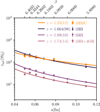
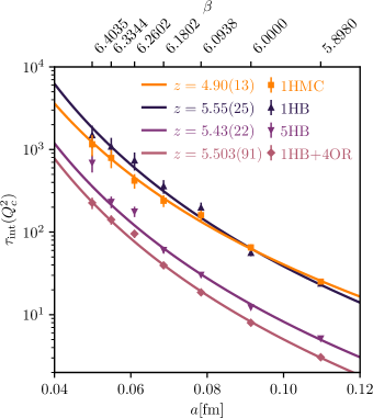
Figure 1: Scaling of the integrated autocorrelation times of square $2\times 2$ Wilson loops $\mathcal{W}_{2,2}$ (left) and the squared topological charge $Q_{c}^{2}$ (right) for different update schemes for the Wilson gauge action. The scaling can be described using a power-law fit equation 20. Details on the simulation parameters are listed in Table 1.

While the integrated autocorrelation times of both observables increase towards finer lattice spacings and are adequately described by a power law behavior, the increase is much steeper for the squared topological charge than for the smeared $2\times 2$ Wilson loops. Below a crossover point at $a\approx$0.08\text{\,}\mathrm{fm}$$, the autocorrelation times of the squared topological charge start to dominate. They can be described by both, a dynamical critical exponent $z\approx 5$ or, alternatively, by an exponential increase, that was first suggested in [17]. This behavior is compatible with the observations in [18].

In contrast, the autocorrelation time of Wilson loops is compatible with a much smaller exponent $z\approx$ $12$. As can be seen in Table 3, the critical exponent does not change significantly with the size of the Wilson loop after 31 stout smearing steps. Generally, the integrated autocorrelation times of smeared Wilson loops slightly increase both with the size of the loops and the number of smearing levels. The only exception to this behavior occurs for larger loops, where a few steps of smearing are required to obtain a clean signal and not measure the autocorrelation of the noise instead.

Regarding the different update algorithms, the unit length HMC does show a somewhat better scaling behavior for all observables than the local update algorithms, but it is also about a factor 7 more computationally expensive per update step (see Table 2). For all local update algorithms considered here, the critical exponents are very similar, but the combination of one heat bath and four overrelaxation steps has the smallest prefactor. It is interesting to note, that this algorithm is also faster by more than a factor 2 than the five-step heat bath update scheme, which does not profit from the inclusion of overrelaxation steps. The single step heat bath without overrelaxation, although numerically cheaper, does have the worst prefactor of the local update algorithms.

Table 2: Relative performance of the update algorithms used in our scaling runs. The results cited here are from the $22^{4}$ lattices. Note that the performance of the heat bath algorithm is slightly better for larger $\beta$, due to the more efficient sampling of the probability distribution (cf. [4, 5]).

Update scheme	Relative time
1HMC	6.98
1HB	1.00
5HB	4.99
1HB+4OR	2.02

Table 3: The dynamical critical exponents obtained from power law fits to the integrated autocorrelation times of $Q_{c}^{2}$, $S_{w}$, and Wilson loops of different sizes after 31 stout smearing steps. Notably, the dynamical critical exponents associated with $Q_{c}^{2}$ are much larger than those associated with the smeared action or smeared Wilson loops of different sizes.

Update	$z(Q_{c}^{2})$	$z(S_{w})$	$z(\mathcal{W}_{2})$	$z(\mathcal{W}_{4})$	$z(\mathcal{W}_{8})$
scheme
1HMC	$4.90(13)$	$1.27(12)$	$1.23(12)$	$1.16(12)$	$1.29(16)$
1HB	$5.55(25)$	$1.69(10)$	$1.66(10)$	$1.64(9)$	$1.82(12)$
5HB	$5.43(22)$	$1.92(11)$	$1.89(10)$	$1.85(10)$	$1.95(10)$
1HB+4OR	$5.50(9)$	$1.77(15)$	$1.74(14)$	$1.71(14)$	$1.85(13)$

Note that the reported numbers differ from those in [82] due to a different fit ansatz (in the proceedings, the fit ansatz included an additional constant term).

For the DBW2 action, the problem is more severe. Figure 2 shows the time series of the topological charge for two runs using the 1HB+4OR and the 1HMC update scheme. Both simulations were done on a $16^{4}$ lattice at $\beta=1.25$ using the DBW2 action.

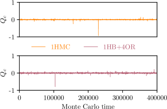
Figure 2: Time series of the topological charge for $V=16^{4}$, $\beta=1.25$ using the DBW2 action. The configurations were generated with the 1HB+4OR update scheme (top) and the 1HMC (bottom). Out of a total of 400000 each, only a single configuration during the 1HB+4OR run and two (successive) configurations during the 1HMC run fulfill the condition $\absolutevalue{Q_{c}}>0.5$.

Evidently, both update schemes are unable to tunnel between different topological sectors in a reasonable time. Only a single configuration during the 1HB+4OR run and two (successive) configurations during the 1HMC run fulfill the condition $\absolutevalue{Q_{c}}>0.5$.

IV.2 Scale setting for the DBW2 action

To the best of our knowledge, scales for the DBW2 action in pure gauge theory have only been computed based on simulations with $\beta\leq 1.22$ [88, 15], and interpolation formulas are only available based on data with $\beta\leq 1.04$ [89]. Since here we perform simulations at $\beta=1.25$, we compute approximate values for $t_{0}$ [90] and $w_{0}$ [91], which allows us to estimate our lattice spacings for comparison to the Wilson results. Both scales are based on the density $E$, which is defined as:

$$E =\frac{1}{4V}\sum\limits_{x\in\Lambda}F_{\mu\nu}^{a}(x)F_{\mu\nu}^{a}(x)$$ (21)

$$=-\frac{1}{2V}\sum\limits_{x\in\Lambda}\tr[F_{\mu\nu}(x)F_{\mu\nu}(x)]$$

Similar to the topological charge definitions, we adopt a plaquette- and clover-based definition of the field strength tensor, with the only difference being that the components are also made traceless, and not just anti-hermitian. The gradient flow scales $t_{0}$ and $w_{0}$ are both defined implicitly:

$$\mathcal{E}(t)=t^{2}\langle E\rangle \Big{|}_{t=t_{0}} =0.3$$ (22)

$$W(t)=t\frac{\mathrm{d}}{\mathrm{d}t}\mathcal{E}(t) \Big{|}_{t=w_{0}^{2}} =0.3$$ (23)

The flow equation was integrated using the third-order commutator free Runge-Kutta scheme from [90] with a step size of $\epsilon=0.025$. Measurements of the clover-based energy density were performed every 10 integration steps, and $t^{2}\langle E(t)\rangle$ was fitted with a cubic spline, which was evaluated with a step size of 0.001. For every value of $\beta$, two independent simulations with 100 measurements each were performed on $48\times 32^{3}$ lattices. Every measurement was separated by 200 update sweeps with the previously described 1HB+4OR update scheme, and the initial 2000 updates were discarded as thermalization phase. Our results are displayed in Table 4.

Table 4: Results for different gradient flow scales for the DBW2 gauge action. These results should not be interpreted as an attempt at a precise scale determination, but rather only serve as an approximate estimate.

$\beta$	$N_{t}\times N_{x}^{3}$	$t_{0,\textrm{plaq}}/a^{2}$	$t_{0,\textrm{clov}}/a^{2}$	$w_{0,\textrm{plaq}}/a^{2}$	$w_{0,\textrm{clov}}/a^{2}$
1.04	$48\times 32$	$3.445(3)$	$3.647(3)$	$3.601(4)$	$3.641(4)$
1.10	$48\times 32$	$4.483(6)$	$4.684(6)$	$4.675(9)$	$4.716(9)$
1.15	$48\times 32$	$5.549(9)$	$5.751(10)$	$5.787(14)$	$5.827(14)$
1.16	$48\times 32$	$5.761(9)$	$5.962(9)$	$5.992(15)$	$6.032(15)$
1.17	$48\times 32$	$6.032(8)$	$6.234(8)$	$6.291(14)$	$6.332(13)$
1.18	$48\times 32$	$6.269(13)$	$6.470(14)$	$6.525(24)$	$6.566(24)$
1.19	$48\times 32$	$6.524(10)$	$6.726(10)$	$6.803(12)$	$6.844(12)$
1.20	$48\times 32$	$6.798(15)$	$7.000(15)$	$7.082(20)$	$7.123(20)$
1.21	$48\times 32$	$7.047(16)$	$7.248(16)$	$7.331(25)$	$7.372(25)$
1.22	$48\times 32$	$7.386(23)$	$7.588(24)$	$7.710(35)$	$7.751(35)$
1.23	$48\times 32$	$7.642(23)$	$7.844(24)$	$7.954(35)$	$7.995(35)$
1.24	$48\times 32$	$7.963(23)$	$8.165(23)$	$8.293(35)$	$8.334(35)$
1.25	$48\times 32$	$8.312(27)$	$8.515(28)$	$8.681(37)$	$8.721(37)$

Using the physical values from [92], these results imply a physical volume of approximately $($0.95\text{\,}\mathrm{fm}$)^{4}$ and a temperature of around $207\text{\,}\mathrm{MeV}$ for the $16^{4}$ lattice from the previous section.

In order to facilitate comparison with other results, we also provide an interpolation of our lattice spacing results. For this purpose, we use a rational fit ansatz with three fit parameters

$$\log(t_{0}/a^{2})=\frac{8\pi^{2}}{33}\beta\frac{1+d_{1}/\beta+d_{2}/\beta^{2}}{1+d_{3}/\beta}$$ (24)

that is asymptotically consistent with perturbation theory [84] and has a sufficient number of degrees of freedom to describe our data well. For our reference, clover-based $t_{0}$ scale setting, this results in a fit with $\chi^{2}/\mathrm{d.o.f.}\approx 1.31$ and parameters $d_{1}\approx 1.0351$, $d_{2}\approx-1.3763$, $d_{3}\approx 0.4058$, which is displayed in Figure 3.

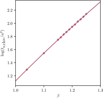
Figure 3: Rational fit of the form Equation 24 to the $t_{0,\textrm{clov}}/a^{2}$ values presented in Table 4. The fit has $\chi^{2}/\mathrm{d.o.f.}\approx 1.31$ and parameters $d_{1}\approx 1.0351$, $d_{2}\approx-1.3763$, and $d_{3}\approx 0.4058$. Error bars are substantially smaller than the symbols.

We want to emphasize that these results are not meant to be an attempt at a precise scale determination, but rather only serve as an approximate estimate. Especially for the finer lattices, the proper sampling of the topological sectors can not be guaranteed, and the comparatively small volumes may introduce non-negligible finite volume effects.

V Results with Metadynamics

Figure 4 shows the time series of the topological charge from simulations with the HMC and the MetaD-HMC with five and ten stout smearing steps on a $22^{4}$ lattice at $\beta=6.4035$, using the Wilson gauge action.

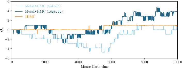
Figure 4: Comparison of the time series of the topological charge between runs using the HMC algorithm and MetaD-HMC runs for $V=22^{4}$, $\beta=6.4035$, using the Wilson gauge action. Both Metadynamics runs are able to transition between topological sectors numerous times, whereas the run using the conventional HMC is essentially stuck in two sectors.

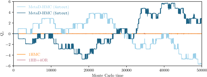
Figure 5: Comparison of the time series of the topological charge between runs using conventional update algorithms (HMC and a combination of heat bath and overrelaxation updates) and MetaD-HMC runs for $V=16^{4}$, $\beta=1.25$, using the DBW2 action. The results shown for the 1HMC and 1HB+4OR update schemes are from the same runs as the time series shown in Figure 2. While the conventional update algorithms are unable to escape the $Q=0$ sector, both Metadynamics runs frequently transition between different topological sectors.

Both MetaD-HMC runs tunnel multiple times between different topological sectors, whereas the conventional HMC essentially displays a single tunneling event between sectors $Q=0$ and $Q=1$. A noteworthy difference between the two MetaD-HMC runs is the increase of fluctuations with higher amounts of smearing. If too many smearing steps are used to define the CV, the resulting $Q$ values will generically be closer to integer, so more simulation time is spent in the sector boundary regions. This will eventually drive the system to coarser regions of configuration space. Since these regions do not contribute significantly to expectation values in the path integral, it is desirable to minimize the time that the algorithm spends there. This is directly related to the issue of small effective sample sizes, which we will discuss in more detail in Section V.2.

A similar comparison for the DBW2 action can be seen in Figure 5. Here, two MetaD-HMC runs with four and five stout smearing steps on a $16^{4}$ lattice at $\beta=1.25$ are compared to the 1HMC and 1HB+4OR runs, which were already shown in Figure 2. Both conventional update schemes are confined to the zero sector, whereas the two MetaD-HMC runs explore topological sectors up to $\absolutevalue{Q}=6$. More quantitatively, the integrated autocorrelation time of $Q_{c}^{2}$ on the DBW2 stream is estimated to be $\tau_{\textrm{int}}(Q_{c}^{2})=$2188(478)$$ for the MetaD-HMC algorithm with 4 smearing steps, whereas lower bounds for the autocorrelation times for the 1HMC and 1HB+4OR update schemes are $4\text{\times}{10}^{5}$, which implies a difference of more than two orders of magnitude.

To illustrate the role of the CV $Q_{\textrm{meta}}$, it may be helpful to compare the time series of $Q_{\textrm{meta}}$ and $Q_{c}$, as shown in Figure 6.

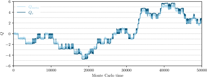
Figure 6: Time series of the CV $Q_{\textrm{meta}}$ and the topological charge $Q_{c}$, measured after 5 and 30 stout smearing steps with a smearing parameter of $\rho=0.12$ respectively. The data is from the same MetaD-HMC run as shown in Figure 5.

The two observables are clearly correlated, but $Q_{\textrm{meta}}$ is distributed more evenly between integers.

V.1 Computational overhead and multiple timescale integration

A fair comparison of the different update schemes also needs to take the computational cost of the algorithms into account. Table 5 shows the relative timings for the different update schemes used here, measured for simulations carried out on $16^{4}$ lattices.

Table 5: Relative timings for the different update schemes measured for simulations carried out on $16^{4}$ lattices. The significant computational overhead for the Metadynamics updates compared to the other algorithms is due to the stout smearing and the stout force recursion required for the Metadynamics force calculation.

Update scheme	Relative time
	Wilson action	DBW2 action
1HB+4OR	1	1
1HMC	3.56	4.46
MetaD-HMC (4stout)	95.48	31.03
MetaD-HMC (5stout)	114.02	36.37

While the MetaD-HMC was not optimized for performance, it is still clear that the additional overhead introduced by the computation of the Metadynamics force contribution is significant for pure gauge theory. The relative overhead is especially large compared to local update algorithms, which are already more efficient than the regular HMC. Note, however, that due to its more non-local character, the relative loss in efficiency when switching to Metadynamics from either a local update algorithm or HMC, is already noticeably smaller for the DBW2 gauge action. Since the majority of the computational overhead comes from the Metadynamics force contribution, and the involved scales are different from those relevant for the gauge force, it seems natural to split the integration into multiple timescales in a similar fashion to the Sexton-Weingarten scheme [93]: The force contributions from the bias potential are correlated to the topological charge, which is an IR observable, whereas the gauge force is usually dominated by short-range, UV fluctuations. Therefore, it is conceivable that integrating the Metadynamics force contribution on a coarser timescale than the gauge force could significantly decrease the required computational effort, while still being sufficiently accurate to lead to reasonable acceptance rates.

We have attempted to use combinations of both the Leapfrog and the Omelyan-Mryglod-Folk second-order integrator with the Omelyan-Mryglod-Folk fourth-order minimum norm integrator. Unfortunately, we were unable to achieve a meaningful reduction of Metadynamics force evaluations without encountering integrator instabilities and deteriorating acceptance rates. However, this approach might still be helpful for simulations with dynamical fermions, where it is already common to split the forces into more than two levels.

Even if such a multiple timescale approach should prove to be unsuccessful in reducing the number of Metadynamics force evaluations, we expect the relative overhead of Metadynamics to be much smaller for simulations including dynamical fermions. In previous studies [41], it was found that compared to conventional HMC simulations, simulations with Metadynamics and 20 steps of stout smearing were about three times slower in terms of real time.

V.2 Scaling of the reweighting factor and improvements to the bias potential

Due to the inclusion of the bias potential, expectation values with respect to the original, physical probability density are obtained by reweighting. As with any reweighting procedure, the overlap between the sampled distribution and the distribution of physical interest needs to be sufficiently large for the method to work properly. A common measure to quantify the efficiency of the reweighting procedure is the effective sample size (ESS), defined as

$$\textrm{ESS}=\frac{\left(\sum\limits_{i}w_{i}\right)^{2}}{\sum\limits_{i}w_{i}^{2}},$$ (25)

where $w_{i}$ is the respective weight associated with each individual configuration. In the case of Metadynamics, this is simply $e^{V(Q_{\textrm{meta},i})}$. We found the normalized ESS, i.e. the ESS divided by the total number of configurations, to generally be of order $\mathcal{O}(10^{-2})$ or lower when simulating in regions of parameter space, where conventional algorithms fail to explore topological sectors other than $Q=0$.

Although the low ESS ultimately results from the fact, that the bias potential is constructed in such a way as to have a marginal distribution over the CV that is flat, we can nonetheless distinguish two parts of this effect. On the one hand, there is the inevitable flattening of the intersector barriers by the bias potential, which is necessary to facilitate tunneling between adjacent topological sectors. On the other hand, however, the different weight of the different topological sectors is also cancelled by the bias potential. While it is necessary for a topology changing update algorithm to reproduce the intersector barriers faithfully, the leveling of the weights of the different topological sectors is entirely unwanted. It enhances the time that the simulation spends at large values of $\absolutevalue{Q}$, so that these sectors are overrepresented compared to their true statistical weight. It is therefore conceivable, that by retaining only the intersector barrier part of the bias potential, the relative weights of the different topological sectors will be closer to their physical values, and the ESS will increase. In previous tests in 2-dimensional U(1) gauge theory, we found that the bias potentials could be described by a sum of a quadratic and multiple oscillating terms [94]:

$$V(Q)=AQ^{2}+\sum\limits_{i=1}^{N}B_{i}\sin^{2}(\pi f_{i}Q)$$ (26)

Here, we fit our bias potentials, that are obtained from the 2-dimensional U(1) simulations, to this form. We then obtain a modified bias potential by subtracting the resulting quadratic term from the data. This modification of the bias potential is effective in reducing the oversampling of topological sectors with large $|Q|$, as evidenced by the larger normalized ESS in Table 6. The resulting marginal distribution over the topological charge is then no longer expected to be constant, but rather resemble a parabola.

Here and in Section VI of this work, we perform scaling tests of the proposed improvements in 2-dimensional U(1) gauge theory, where high statistics can be generated more easily than in 4-dimensional $SU(3)$ gauge theory. The action is given by the standard Wilson plaquette action

$$S_{g}=\beta\sum\limits_{n\in\Lambda}\left(1-\real[P_{t,x}(n)]\right),$$ (27)

and updates are performed with a single-hit Metropolis algorithm. The topological charge is defined using a geometric, integer-valued definition:

$$Q=\frac{1}{2\pi}\imaginary[\sum\limits_{n\in\Lambda}\log P_{t,x}(n)\Bigr{]}$$ (28)

For all Metadynamics updates, we use a field-theoretic definition of the topological charge that is generally not integer-valued:

$$Q_{\textrm{meta}}=\frac{1}{2\pi}\imaginary\left[\sum\limits_{n\in\Lambda}P_{t,x}(n)\right]$$ (29)

Since the charge distributions obtained from the two definitions already show reasonable agreement without any smearing for the parameters considered here, we can use local update algorithms and directly include the Metadynamics contribution in the staple. A similar idea that encourages tunneling in the Schwinger model by adding a small modification to the action was proposed in [95].

Table 6 contains the relative ESS and integrated autocorrelation times for different lattice spacings on the same line of constant physics in 2-dimensional U(1) theory. We compare Metadynamics runs using bias potentials obtained directly from previous simulations with Metadynamics runs using potentials that were modified to retain the relative weights of the topological sectors as described above.

Table 6: Normalized effective sample sizes for different lattices on the same line of constant physics in 2-dimensional U(1) gauge theory. Overall, $10^{7}$ measurements were performed with a separation of 10 update sweeps between every measurement. More details on the simulation setup can be found in Section VI.2.

$L/a$	$\beta$	$\textrm{ESS}/n_{\textrm{meas}}$	$\tau_{\textrm{int}}(Q^{2})$
Regular bias potential
16	3.2	0.33088(74)	53
20	5.0	0.2181(11)	208
24	7.2	0.1270(11)	568
28	9.8	0.08805(81)	677
32	12.8	0.08261(85)	1168
Modified bias potential
16	3.2	0.9950627(11)	6
20	5.0	0.643084(87)	34
24	7.2	0.28572(12)	124
28	9.8	0.27291(16)	228
32	12.8	0.18751(25)	248

We see large improvements for both the ESS and $\tau_{\textrm{int}}$ in the modified case, even for the finest lattices considered.

We expect that the quadratic term is mostly relevant for small volumes and high temperatures. With larger volumes and lower temperatures, the slope should decrease, and with it the importance of correctly capturing this term. On the other hand, the oscillating term is expected to grow more important with finer lattice spacings, as the barriers between the different sectors grow steeper. Thus, the oscillating term needs to be described more and more accurately towards the continuum.

A standard technique to decrease, but not completely eliminate, action barriers is well-tempered Metadynamics [96].In this approach, the height of the added Gaussians $w$ decays with increasing potential. In our tests, we found that this method does increase the ESS, but at the cost of higher autocorrelation times to the point where any gains from the ESS that would be visible in the uncertainties of observables are nullified. Although it might still have some use in accelerating the build-up process or as a possible intermediate stream for PT-MetaD (see Section VI), we decided not to explore this option further at this point.

V.3 Accelerating the equilibration/buildup of the bias potential

Another avenue of improvement is accelerating the build-up of the bias potential, for which we again explore two possible ideas. This aspect becomes especially relevant when considering large-scale simulations, where runs are often limited to $\mathcal{O}(10^{4})$ update sweeps, and a lengthy buildup phase of the bias potential would render the method infeasible.

The first idea is to exploit the aforementioned well-tempered variant of Metadynamics, by choosing a larger starting value of the Gaussian height $w$ and letting it decay slowly so as to minimize the change in the potential that arises from the decay. While this approach adds another fine-tunable parameter, namely the decay rate, we found that this did indeed significantly cut down on the number of update iterations required to thermalize the potential. A small caveat is, that in order to choose the optimal decay rate, one would have to have knowledge on the approximate height of the action barriers, which is not always the case.

A way of improving the build-up time without any prior knowledge of the bias potential is to use an enhancement of Metadynamics which is most commonly referred to as multiple walkers Metadynamics [97], where the potential is simultaneously built up by several independent streams in a trivially parallelizable way. To add to this, we make each stream start in a distinct topological sector by the use of instanton configurations, which can easily be constructed in 2-dimensional U(1) gauge theory [98]. Namely, an instanton configuration with charge $Q$ is given by

$$U_{t}^{I}(Q;t,x) =\exp\left(-2\pi ix\frac{Q_{j}}{N_{x}N_{t}}\right),$$ (30)

$$U_{x}^{I}(Q;t,x) =\exp\left(2\pi it\frac{Q_{j}}{N_{t}}\delta_{x,N_{x}}\right).$$

The parallel and serial build are compared in Figure 7 where the potential parameters for each stream are given by: $Q_{\textrm{max/min}}=\pm 7$, $n_{\textrm{bins}}=1400$ and $w=0.002$.

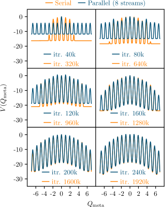
Figure 7: Comparison of serial and parallel build of the bias potential in 2-dimensional U(1) gauge theory for $32^{2}$ lattices. The ratio of update iterations was held fixed at 8:1, so that both methods would use the same number of total update steps during each snapshot.

Since this method is an embarrassingly parallel task, we expect it to easily carry over to higher-dimensional, non-abelian theories with topological properties. In the case of 4-dimensional SU(3) the direct construction of instantons with higher charge is not quite as simple as in 2-dimensional U(1) gauge theory. The construction of lattice instantons with even charge is described in [98], and lattice instantons with odd charge can be constructed by combining multiple instantons with charge $Q=1$ [99, 82]. Regardless, having exact instantons is not required, since we only need each stream to start in a sector, where it is then very likely to fall into the local minimum of the specified sector.

Independent of the possible improvements mentioned here, a fine-tuning of the standard Metadynamics parameters could also prove to be worthwhile in regard to accelerating the buildup and improving the quality of the bias potential.

VI Combining Metadynamics with parallel tempering

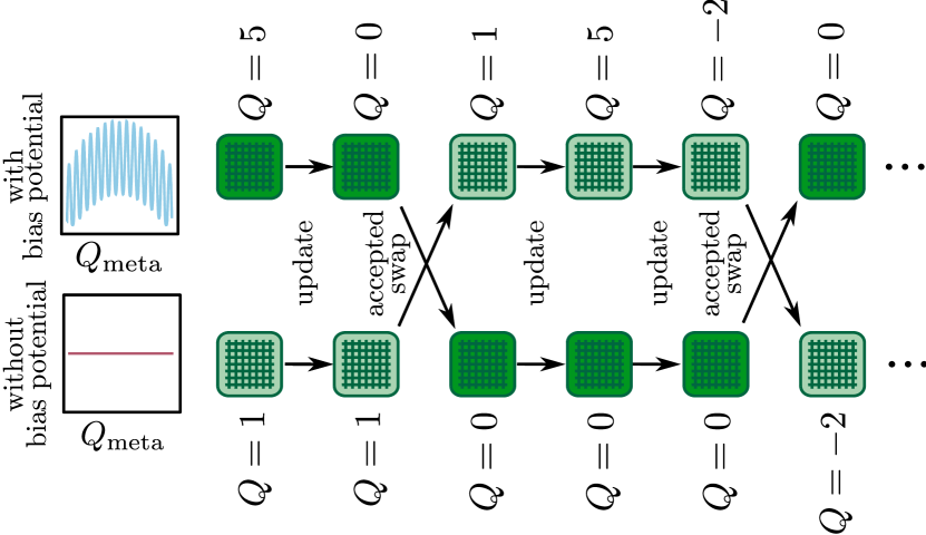
Figure 8: Illustration of the proposed PT-MetaD algorithm. The upper row shows the run with an active bias potential, whereas the lower row shows the run without an active bias potential. The plots on the left indicate the bias potential as a function of the continuous observable $Q_{\text{meta}}$. The green squares symbolize gauge configurations. Different shades are to guide the eyes. The indicated integer charges $Q$ show the sector the configuration belongs to and are not the same as the CVs. The values of $Q$ are for illustration only and not actual data. Red dots indicate the value of the CV. The frequency of sector changes in the upper row is exaggerated.

In order to eliminate the problem of small effective sample sizes observed in our Metadynamics simulations due to the required reweighting, we propose to combine Metadynamics with parallel tempering [70]. This is done in a spirit similar to the parallel tempering on a line defect proposed by Hasenbusch [30]. We introduce two simulation streams: One with a bias potential, and the other without it, while actions $S(U)$ are the same for both streams. Note that since we are working in pure gauge theory, this means the second stream without bias potential can be updated with local update algorithms. After a fixed number of updates have been performed on the two streams, a swap of the two configurations is proposed and subject to a standard Metropolis accept-reject step, with the action difference given by

$$\Delta S^{M}_{t} =[S^{M}_{t}(U_{1})+S(U_{2})]-[S^{M}_{t}(U_{2})+S(U_{1})]$$ (31)

$$=V_{t}(Q_{\textrm{meta},1})-V_{t}(Q_{\textrm{meta},2}),$$

where the indices of the quantities denote the number of the stream and $V_{t}$ is the bias potential in the first stream. It is apparent and important to note that the action difference is simple to compute regardless of what the physical action looks like. Even in simulations where dynamical fermions are present, the contributions from the physical action are always cancelled out by virtue of the two streams having the same action parameters; only the contribution from the Metadynamics bias potential remains.

Since the second stream samples configurations according to the (physical) target distribution, no reweighting is needed and thus the effective sample size is not reduced. Additionally, if the swaps are effective, this stream will inherit the topological sampling from the stream with bias potential and thus also sample topological sectors well. Effectively, the accept-reject step for swap proposals serves as a filter for configurations with vanishing statistical weight, thereby decreasing the statistical uncertainties on all observables weakly correlated to the topological charge. What remains to be seen is, whether the efficiency of the sampling of the topological sectors carries over from the Metadynamics stream to the measurement stream. In this section, we address this question both via a scaling test in 2-dimensional U(1) and with exploratory runs in 4-dimensional SU(3) with the DBW2 gauge action in a region where conventional update algorithms are effectively frozen.

VI.1 Scaling tests in 2-dimensional U(1)

We carried out a number of simulations in 2-dimensional $U(1)$ gauge theory for several lattice size and couplings with the same parameters as used in the test described in Section V.2. We use the potentials already build for these Metadynamics runs as static bias potentials in a number of parallel tempered Metadynamics runs. For each set of parameters, we carry out one run with the respective unmodified potential and one run with a potential modified as described in Section V.2. In these runs, swaps between the two streams were proposed after each had completed a single update sweep over all lattice sites. well as the resulting autocorrelation times of the topological charge $Q$ can be found in Table 7. To ensure that actual tunneling occurs, we also monitor the sum of the squared topological charges on both streams. This observable allows us to distinguish the fluctuations in $Q$ originating from true tunneling events, mostly appearing in the stream with bias potential, from repeated swaps between the two streams without tunneling, which might also introduce a fluctuation of $Q$ in the streams without actually overcoming any potential barriers.

Table 7: Integrated autocorrelation times for different lattices on the same line of constant physics in 2-dimensional U(1) gauge theory, using both Metropolis and PT-MetaD updates. Observables indexed with $1$ are taken from the stream with bias potential, whereas those indexed with $2$ are taken from the regular stream. Overall, $10^{7}$ measurements were performed with a separation of 10 update sweeps between every measurement.

$N$	$\beta$	$\tau_{\textrm{int}}(Q_{2}^{2})$	$\tau_{\textrm{int}}(Q_{1}^{2}+Q_{2}^{2})$
Conventional updates
16	3.2	4	-
20	5.0	72	-
24	7.2	3940	-
28	9.8	462473	-
32	12.8	-	-
PT-MetaD (regular bias potential)
16	3.2	6	21
20	5.0	60	143
24	7.2	940	535
28	9.8	1731	819
32	12.8	1927	1320
PT-MetaD (modified bias potential)
16	3.2	5	6
20	5.0	48	48
24	7.2	185	209
28	9.8	317	404
32	12.8	313	466

Figure 9 shows the scaling of the total amount of independent configuration, which is given by the quotient of the effective sample size Equation 25 and the integrated autocorrelation time of the topological susceptibility. The performance of the standard Metropolis algorithm is compared to parallel tempered and standard Metadynamics, with both modified (see Section V.2) and non-modified bias potentials. Clearly, the parallel tempered Metadynamics update schemes perform best for small lattice spacings. Most importantly, the ratio of independent configurations in the sample seems to reach a plateau for finer lattice spacings, which is in stark contrast to conventional Metadynamics. It is also worth noting, that the modified bias potential provides better results than the non-modified one. This is consistent with our expectation, that large excursions in the topological charge, which produce irrelevant configurations, are curbed by the modified bias potential.

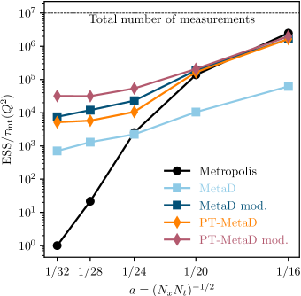
Figure 9: Continuum scaling of the total sample size for the standard Metropolis algorithm and variations of MetaD-Metropolis in 2-dimensional U(1) from Table 6 and Table 7. The lines are drawn to guide the eyes.

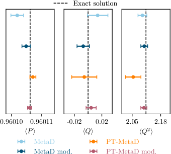
Figure 10: Comparison of expectation values and uncertainties for the plaquette (left), the topological charge (middle), and the topological susceptibility (right) for the standard Metropolis algorithm and variations of MetaD-Metropolis in 2-dimensional U(1) for $32^{2}$ lattices and $\beta=12.8$. The dashed lines correspond to the exact solutions [100, 101, 102].

For a more detailed look at the effectiveness of the new algorithm, Figure 10 compares the results of parallel tempered Metadynamics with those of standard Metadynamics at our finest lattice, with and without modification of the bias potential, and with the exact solutions [100, 101, 102]. First we note, that there is no significant difference in the performance between standard and parallel tempered Metadynamics in the topology related observables $Q$ and $Q^{2}$, at least in the case of a modified bias potential. This is a very encouraging result, since the topological sampling of parallel tempered Metadynamics can not possibly exceed that of standard Metadynamics, as ultimately it is inherited from there. On the other hand, the inclusion of the irrelevant higher sectors with the unmodified bias potential does increase the error bars and there is some indication, that not all of the topological sector sampling is carried over into the measurement run of parallel tempered Metadynamics. Looking at an observable which is not related to topology, such as the plaquette, reveals that parallel tempered Metadynamics is superior to pure Metadynamics. This is clearly the effect of the better effective sample size and the larger number of independent configurations.

In summary, our scaling tests in 2-dimensional U(1) suggest, that parallel tempered Metadynamics with a modified bias potential has a much improved topological sampling, which seems to be almost equivalent to standard Metadynamics, while at the same time not suffering from a reduced effective sample size. There is some indication, that the ratio of independent to total configurations does reach a stable plateau in the continuum limit. These results encourage us to perform an exploratory study in pure SU(3) gauge theory in 4 dimensions.

VI.2 First results in 4-dimensional SU(3)

For our exploratory study in 4-dimensional SU(3), we turn to the DBW2 gauge action at $\beta=1.25$ on a $V=16^{4}$ lattice, which we have already used in Section V. For our first run, which is depicted in the left panels of Figure 12, we have combined a local 1HB+4OR measurement run with a 4stout MetaD-HMC run that dynamically generates the bias potential. Between swap proposals, updates for the two streams are performed at a ratio of 10 (1HB+4OR) to 1 (MetaD-HMC), which roughly reflects the relative wall clock times between the algorithms. One can see that the measurement run starts exploring other topological sectors almost as soon as the parallel run with active bias potential has gained access to them.

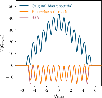
Figure 11: Comparison between the original bias potential and its trend subtracted modifications from singular spectrum analysis and piecewise subtraction of the $Q^{2}$ term.

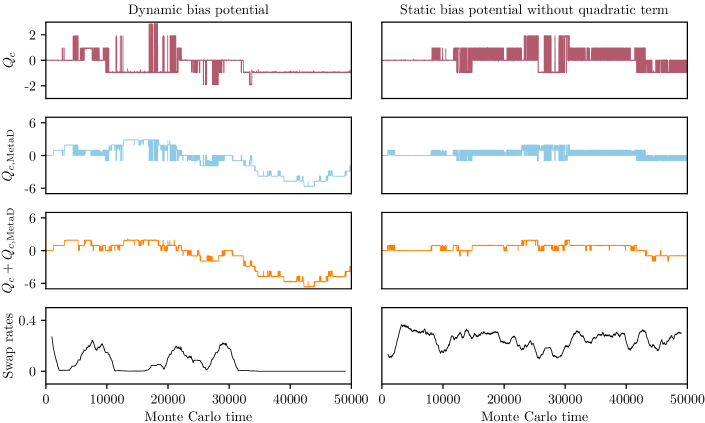
Figure 12: Topological charge vs. Monte Carlo time for our parallel Metadynamics runs on a $V=16^{4}$ lattice at $\beta=1.25$ with DBW2 gauge action and 4 steps of stout smearing in the definition of $Q_{\textrm{meta}}$. The left panel shows results of our first run with a dynamically built bias potential, while the right-hand side shows our second run with a static one. The topmost row shows the time series of the topological charges in the respective measurement runs, while the second row is for the Metadynamics part. The third row displays the sum of the topological charges of the measurement and Metadynamics part of the runs, thus indicating genuine transitions of the entire system into new topological sectors. In the bottom row, the running average of the swap acceptance rate with a window size of 2000 is displayed.

In the later stages of the run, when the bias potential is sufficiently built up to allow the Metadynamics run to enter higher topological sectors, one can see that the swap rate is lowered by the action difference between the topological sectors, leading to an overall swap rate of $\sim 0.063$. This effect mirrors the reduction of the effective sample size in pure Metadynamics updates and may be ameliorated by removing the quadratic term in the bias potential, as discussed in Section V.2. In fact, the relevant point is that the action difference between the maxima of the bias potential for different topological sectors reflects the relative weight of these sectors in the path integral and should not be flattened out. Ideally, we want the bias potential to only reproduce the barriers between the sectors, not their relative weights. For a second exploratory parallel Metadynamics run, we therefore opted for a static bias potential of this sort. Lacking data that are precise enough to model the bias potential in detail, as we did in 2-dimensional U(1), we started from the bias potential of a previous Metadynamics run and extracted the high frequency (in the CV) part of the topological barriers, while eliminating the long range part corresponding to the relative weight of the topological sectors. For this purpose, we chose to perform a singular spectrum analysis (SSA) [103] and crosschecked the result with a simple, piece-wise subtraction of the $Q^{2}$ term between consecutive local maxima. As displayed in Figure 11, both methods result in a similar modified bias potential that seems to reproduce the intersector barriers rather well.

The right panels of Figure 12 display the results of the corresponding parallel tempered Metadynamics run. As one can see, large topological charge excursions of the Metadynamics run are now curbed, and the swap acceptance rate has increased to $\sim 0.25$. In addition, the acceptance rate is approximately constant over the entire run, as it should be expected for a static bias potential. We would like to emphasize, that the bias potential we extracted is a rather rough guess. With a larger amount of data, it might be possible to extract a better bias potential, possibly leading to even better acceptance rates. Considering the rather simple ultimate form of the bias potential used, it might also be possible to model it with sufficient accuracy for a good initial guess at other run parameters. We plan to address these points in a future publication.

In any case, these first results clearly show that the parallel tempered Metadynamics algorithm is able to achieve enhanced topological sampling in 4-dimensional SU(3) without the reduction of the effective sample size that is typical for algorithms with a bias potential.

VII Conclusion and outlook

In this paper, we have demonstrated that Metadynamics can be used to significantly reduce the integrated autocorrelation times of topological quantities in lattice simulations. In simulations of 4-dimensional SU(3) gauge theory with the DBW2 action, we have observed reductions of the autocorrelation times of more than two orders of magnitude. However, the direct application of Metadynamics is not entirely unproblematic: Compared to local update algorithms, there is a large computational overhead due to the costly Metadynamics force evaluations, and the reweighting procedure required to obtain unbiased expectation values can significantly reduce the effective sample size. In order to circumvent this reduction, we have proposed two improvements: The first consists of modifying the bias potential, so that all topological sectors are represented with their correct weight; the second is adding a dedicated measurement stream parallel to the Metadynamics run, which uses a conventional update algorithm. Periodically, swaps between the two streams are suggested and subject to an accept-reject step. The accept-reject step during swap proposals then effectively serves as a filter for configurations with low statistical weight. This parallel tempered Metadynamics algorithm, including both improvements, has been successfully applied to 4-dimensional SU(3) gauge theory. Furthermore, scaling tests in 2-dimensional U(1) gauge theory indicate gains of more than an order of magnitude compared to standard Metadynamics, and an improved scaling of autocorrelation times with the lattice spacing compared to standard update algorithms. Additionally, we have demonstrated that the buildup of the Metadynamics bias potential may be accelerated by running multiple Metadynamics simulations in parallel.

We believe these results are promising, and plan to study the scaling behavior of the methods tested here in more detail for 4-dimensional SU(3) gauge theory, and eventually in full QCD. Conceptually, there seem to be no obstacles for implementing parallel tempered Metadynamics in full QCD. We also plan to explore possible optimizations for parallel tempered Metadynamics. These include optimizing the bias potential via enhanced buildup and extraction and, possibly, describing it parametrically. Furthermore, it would be interesting to investigate whether adding intermediate runs to a parallel tempered Metadynamics stream could increase performance, despite the additional computational cost.

Appendix A Metadynamics force

In order to obtain an expression for Equation 19, the algebra-valued derivative of $Q_{\textrm{meta}}$ with respect to the unsmeared links $U_{\mu}^{(0)}$ has to be calculated. Here, we will only focus on the derivative of the clover-based topological charge $Q_{c}$ with respect to a fully smeared gauge configuration $U$. For details of the stout-force recursion, we refer to [79, 19].

On the lattice, the following definition holds for a suitably defined lattice field strength tensor:

$$Q_{c}=\frac{1}{32\pi^{2}}\sum\limits_{n\in\Lambda}\tr[\epsilon_{\mu\nu\rho\sigma}F_{\mu\nu}(n)F_{\rho\sigma}(n)]$$ (32)

The lattice field strength tensor based on the clover term is defined as the sum of four plaquettes:

$$F_{\mu\nu}(n)=\frac{-i}{8a^{2}}\left(C_{\mu\nu}(n)-C_{\nu\mu}(n)\right)$$ (33)

where the clover term in turn is defined via:

$$C_{\mu\nu}(n)= P_{\mu,\nu}(n)+P_{\nu,-\mu}(n)$$ (34)

$$+P_{-\mu,-\nu}(n)+P_{-\nu,\mu}(n)$$

For notational purposes, we define the auxiliary variables $R_{\mu\nu}(n)=C_{\mu\nu}(n)-C_{\nu\mu}(n)$ and drop the specification of the lattice site $n$ unless pertinent to the formula.

What we need for the force is the sum over all eight algebra directions:

$$T^{a}\sum\limits_{\nu\rho\sigma}4\partial_{n,\alpha}^{a}\epsilon_{\alpha\nu\rho\sigma}\tr[R_{\alpha\nu}R_{\rho\sigma}]$$ (35)

where the sum over $a$ is implied.

Using the field strength tensor’s symmetry properties, the derivative can be written as a term of the following form:

$$\sum\limits_{\nu\rho\sigma}\partial_{n,\alpha}^{a}\epsilon_{\alpha\nu\rho\sigma}\tr[R_{\alpha\nu}R_{\rho\sigma}] =\sum\limits_{\nu\rho\sigma}\epsilon_{\alpha\nu\rho\sigma}2\real\tr[T^{a}U_{\alpha}(n)U_{\nu}(n+\alpha)U^{\dagger}_{\alpha}(n+\nu)U^{\dagger}_{\nu}(n)R_{\rho\sigma}(n)$$ (36)

$$-T^{a}U_{\alpha}(n)U^{\dagger}_{\nu}(n+\alpha-\nu)U^{\dagger}_{\alpha}(n-\nu)R_{\rho\sigma}(n-\nu)U_{\nu}(n-\nu)$$

$$-T^{a}U_{\alpha}(n)U^{\dagger}_{\nu}(n+\alpha-\nu)R_{\rho\sigma}(n+\alpha-\nu)U^{\dagger}_{\alpha}(n-\nu)U_{\nu}(n-\nu)$$

$$+T^{a}U_{\alpha}(n)R_{\rho\sigma}(n+\alpha)U_{\nu}(n+\alpha)U^{\dagger}_{\alpha}(n+\nu)U^{\dagger}_{\nu}(n)$$

$$-T^{a}U_{\alpha}(n)U^{\dagger}_{\nu}(n+\alpha-\nu)U^{\dagger}_{\alpha}(n-\nu)U_{\nu}(n-\nu)R_{\rho\sigma}(n)$$

$$+T^{a}U_{\alpha}(n)U_{\nu}(n+\alpha)U^{\dagger}_{\alpha}(n+\nu)R_{\rho\sigma}(n+\nu)U^{\dagger}_{\nu}(n)$$

$$-T^{a}U_{\alpha}(n)R_{\rho\sigma}(n+\alpha)U^{\dagger}_{\nu}(n+\alpha-\nu)U^{\dagger}_{\alpha}(n-\nu)U_{\nu}(n-\nu)$$

$$+T^{a}U_{\alpha}(n)U_{\nu}(n+\alpha)R_{\rho\sigma}(n+\alpha+\nu)U^{\dagger}_{\alpha}(n+\nu)U^{\dagger}_{\nu}(n)\Big{]}$$

$$=\sum\limits_{\nu\rho\sigma}\epsilon_{\alpha\nu\rho\sigma}2\real\tr[T^{a}A_{\alpha\nu\rho\sigma}\Big{]}$$

$$=2\real\tr[T^{a}A_{\alpha}\Big{]}$$

An expression of the above form can be rewritten using the projector induced by the scalar product of the algebra:

$$T^{a}\tr[T^{a}A_{\alpha}]=-\frac{1}{2}A_{\alpha}+\frac{1}{6}\tr[A_{\alpha}]$$ (37)

Which in our case translates to:

$$T^{a}2\real\tr[T^{a}A_{\alpha}] =T^{a}\tr[T^{a}A_{\alpha}+(T^{a}A_{\alpha})^{\dagger}\Big{]}$$ (38)

$$=T^{a}\tr[T^{a}A_{\alpha}-T^{a}A_{\alpha}^{\dagger}\Big{]}$$

$$= -\frac{1}{2}(A_{\alpha}-A_{\alpha}^{\dagger})$$

$$+\frac{1}{6}\tr[A_{\alpha}-A_{\alpha}^{\dagger}\Big{]}$$

Including the factor we lost after defining $R_{\mu\nu}$, we obtain the derivative of the trace in Equation 32

$$\sum\limits_{\mu\nu\rho\sigma}T^{a}\partial_{n,\alpha}^{a}\epsilon_{\mu\nu\rho\sigma}\tr[F_{\mu\nu}F_{\rho\sigma}] =\sum\limits_{\mu\nu\rho\sigma}-\frac{1}{64}T^{a}\partial_{n,\alpha}^{a}\epsilon_{\mu\nu\rho\sigma}\tr[R_{\mu\nu}R_{\rho\sigma}]$$ (39)

$$=\frac{1}{32}\Big{(}\big{(}A_{\alpha}-A_{\alpha}^{\dagger}\big{)}-\frac{1}{3}\tr[A_{\alpha}-A_{\alpha}^{\dagger}\big{]}\Big{)}$$

Summarized, the algebra-valued derivative of the clover-based topological charge with respect to the gauge link $U_{\alpha}(n)$ can be written as:

$$T^{a}\partial_{n,\alpha}^{a}Q_{c} =\sum\limits_{\mu\nu\rho\sigma}\frac{1}{32\pi^{2}}T^{a}\partial_{n,\alpha}^{a}\epsilon_{\mu\nu\rho\sigma}\tr[F_{\mu\nu}F_{\rho\sigma}]$$ (40)

$$=\frac{1}{1024\pi^{2}}\Big{(}\big{(}A_{\alpha}-A_{\alpha}^{\dagger}\big{)}$$

$$-\frac{1}{3}\tr[A_{\alpha}-A_{\alpha}^{\dagger}\big{]}\Big{)}$$

References

- Aoki et al. [2022] Y. Aoki et al. (Flavour Lattice Averaging Group (FLAG)), FLAG Review 2021, Eur. Phys. J. C 82, 869 (2022), arXiv:2111.09849 [hep-lat] .
- Creutz [1979] M. Creutz, Confinement and the critical dimensionality of space-time, Phys. Rev. Lett. 43, 553 (1979).
- Creutz [1980] M. Creutz, Monte Carlo Study of Quantized SU(2) Gauge Theory, Phys. Rev. D 21, 2308 (1980).
- Fabricius and Haan [1984] K. Fabricius and O. Haan, Heat Bath Method for the Twisted Eguchi-Kawai Model, Phys. Lett. B 143, 459 (1984).
- Kennedy and Pendleton [1985] A. D. Kennedy and B. J. Pendleton, Improved Heat Bath Method for Monte Carlo Calculations in Lattice Gauge Theories, Phys. Lett. B 156, 393 (1985).
- Cabibbo and Marinari [1982] N. Cabibbo and E. Marinari, A New Method for Updating SU(N) Matrices in Computer Simulations of Gauge Theories, Phys. Lett. B 119, 387 (1982).
- Adler [1981] S. L. Adler, An Overrelaxation Method for the Monte Carlo Evaluation of the Partition Function for Multiquadratic Actions, Phys. Rev. D 23, 2901 (1981).
- Creutz [1987] M. Creutz, Overrelaxation and Monte Carlo Simulation, Phys. Rev. D 36, 515 (1987).
- Brown and Woch [1987] F. R. Brown and T. J. Woch, Overrelaxed Heat Bath and Metropolis Algorithms for Accelerating Pure Gauge Monte Carlo Calculations, Phys. Rev. Lett. 58, 2394 (1987).
- Duane et al. [1987] S. Duane, A. D. Kennedy, B. J. Pendleton, and D. Roweth, Hybrid Monte Carlo, Phys. Lett. B 195, 216 (1987).
- Alles et al. [1996] B. Alles, G. Boyd, M. D’Elia, A. Di Giacomo, and E. Vicari, Hybrid Monte Carlo and topological modes of full QCD, Phys. Lett. B 389, 107 (1996), arXiv:hep-lat/9607049 .
- Orginos [2002] K. Orginos (RBC), Chiral properties of domain wall fermions with improved gauge actions, Nucl. Phys. B Proc. Suppl. 106, 721 (2002), arXiv:hep-lat/0110074 .
- DeGrand et al. [2003] T. A. DeGrand, A. Hasenfratz, and T. G. Kovacs, Improving the chiral properties of lattice fermions, Phys. Rev. D 67, 054501 (2003), arXiv:hep-lat/0211006 .
- Noaki [2003] J. Noaki (RBC), Calculation of weak matrix elements in domain wall QCD with the DBW2 gauge action, Nucl. Phys. B Proc. Suppl. 119, 362 (2003), arXiv:hep-lat/0211013 .
- Aoki et al. [2006] Y. Aoki et al., The Kaon B-parameter from quenched domain-wall QCD, Phys. Rev. D 73, 094507 (2006), arXiv:hep-lat/0508011 .
- Del Debbio et al. [2002] L. Del Debbio, H. Panagopoulos, and E. Vicari, theta dependence of SU(N) gauge theories, JHEP 08, 044, arXiv:hep-th/0204125 .
- Del Debbio et al. [2004] L. Del Debbio, G. M. Manca, and E. Vicari, Critical slowing down of topological modes, Phys. Lett. B 594, 315 (2004), arXiv:hep-lat/0403001 .
- Schaefer et al. [2011] S. Schaefer, R. Sommer, and F. Virotta (ALPHA), Critical slowing down and error analysis in lattice QCD simulations, Nucl. Phys. B 845, 93 (2011), arXiv:1009.5228 [hep-lat] .
- Durr et al. [2011] S. Durr, Z. Fodor, C. Hoelbling, S. D. Katz, S. Krieg, T. Kurth, L. Lellouch, T. Lippert, K. K. Szabo, and G. Vulvert (BMW), Lattice QCD at the physical point: Simulation and analysis details, JHEP 08, 148, arXiv:1011.2711 [hep-lat] .
- Bernard and Toussaint [2018] C. Bernard and D. Toussaint (MILC), Effects of nonequilibrated topological charge distributions on pseudoscalar meson masses and decay constants, Phys. Rev. D 97, 074502 (2018), arXiv:1707.05430 [hep-lat] .
- Borsanyi et al. [2021] S. Borsanyi et al., Leading hadronic contribution to the muon magnetic moment from lattice QCD, Nature 593, 51 (2021), arXiv:2002.12347 [hep-lat] .
- Brower et al. [2003] R. Brower, S. Chandrasekharan, J. W. Negele, and U. J. Wiese, QCD at fixed topology, Phys. Lett. B 560, 64 (2003), arXiv:hep-lat/0302005 .
- Aoki et al. [2007] S. Aoki, H. Fukaya, S. Hashimoto, and T. Onogi, Finite volume QCD at fixed topological charge, Phys. Rev. D 76, 054508 (2007), arXiv:0707.0396 [hep-lat] .
- Lüscher [2018] M. Lüscher, Stochastic locality and master-field simulations of very large lattices, EPJ Web Conf. 175, 01002 (2018), arXiv:1707.09758 [hep-lat] .
- Luscher and Schaefer [2011] M. Luscher and S. Schaefer, Lattice QCD without topology barriers, JHEP 07, 036, arXiv:1105.4749 [hep-lat] .
- Joo et al. [1999] B. Joo, B. Pendleton, S. M. Pickles, Z. Sroczynski, A. C. Irving, and J. C. Sexton (UKQCD), Parallel tempering in lattice QCD with O(a)-improved Wilson fermions, Phys. Rev. D 59, 114501 (1999), arXiv:hep-lat/9810032 .
- Ilgenfritz et al. [2002] E.-M. Ilgenfritz, W. Kerler, M. Muller-Preussker, and H. Stuben, Parallel tempering in full QCD with Wilson fermions, Phys. Rev. D 65, 094506 (2002), arXiv:hep-lat/0111038 .
- Borsanyi et al. [2022] S. Borsanyi, K. R., Z. Fodor, D. A. Godzieba, P. Parotto, and D. Sexty, Precision study of the continuum SU(3) Yang-Mills theory: How to use parallel tempering to improve on supercritical slowing down for first order phase transitions, Phys. Rev. D 105, 074513 (2022), arXiv:2202.05234 [hep-lat] .
- Mages et al. [2017] S. Mages, B. C. Toth, S. Borsanyi, Z. Fodor, S. D. Katz, and K. K. Szabo, Lattice QCD on nonorientable manifolds, Phys. Rev. D 95, 094512 (2017), arXiv:1512.06804 [hep-lat] .
- Hasenbusch [2017] M. Hasenbusch, Fighting topological freezing in the two-dimensional CPN-1 model, Phys. Rev. D 96, 054504 (2017), arXiv:1706.04443 [hep-lat] .
- Endres et al. [2015] M. G. Endres, R. C. Brower, W. Detmold, K. Orginos, and A. V. Pochinsky, Multiscale Monte Carlo equilibration: Pure Yang-Mills theory, Phys. Rev. D 92, 114516 (2015), arXiv:1510.04675 [hep-lat] .
- Detmold and Endres [2016] W. Detmold and M. G. Endres, Multiscale Monte Carlo equilibration: Two-color QCD with two fermion flavors, Phys. Rev. D 94, 114502 (2016), arXiv:1605.09650 [hep-lat] .
- Detmold and Endres [2018] W. Detmold and M. G. Endres, Scaling properties of multiscale equilibration, Phys. Rev. D 97, 074507 (2018), arXiv:1801.06132 [hep-lat] .
- Fucito and Solomon [1984] F. Fucito and S. Solomon, Does standard monte carlo give justice to instantons?, Physics Letters B 134, 230 (1984).
- Smit and Vink [1988] J. Smit and J. C. Vink, Topological Charge and Fermions in the Two-dimensional Lattice U(1) Model. 1. Staggered Fermions, Nucl. Phys. B 303, 36 (1988).
- Dilger [1992] H. Dilger, Screening in the lattice Schwinger model, Phys. Lett. B 294, 263 (1992).
- Dilger [1995] H. Dilger, Topological zero modes in Monte Carlo simulations, Int. J. Mod. Phys. C 6, 123 (1995), arXiv:hep-lat/9408017 .
- Durr [2012] S. Durr, Physics of with rooted staggered quarks, Phys. Rev. D 85, 114503 (2012), arXiv:1203.2560 [hep-lat] .
- Albandea et al. [2021] D. Albandea, P. Hernández, A. Ramos, and F. Romero-López, Topological sampling through windings, Eur. Phys. J. C 81, 873 (2021), arXiv:2106.14234 [hep-lat] .
- Laio et al. [2016] A. Laio, G. Martinelli, and F. Sanfilippo, Metadynamics surfing on topology barriers: the case, JHEP 07, 089, arXiv:1508.07270 [hep-lat] .
- Bonati [2018] C. Bonati, The topological properties of QCD at high temperature: problems and perspectives, EPJ Web Conf. 175, 01011 (2018), arXiv:1710.06410 [hep-lat] .
- Duane et al. [1986] S. Duane, R. Kenway, B. J. Pendleton, and D. Roweth, Acceleration of gauge field dynamics, Physics Letters B 176, 143 (1986).
- Duane and Pendleton [1988] S. Duane and B. J. Pendleton, GAUGE INVARIANT FOURIER ACCELERATION, Phys. Lett. B 206, 101 (1988).
- Davies et al. [1990] C. T. H. Davies, G. G. Batrouni, G. R. Katz, A. S. Kronfeld, G. P. Lepage, P. Rossi, B. Svetitsky, and K. G. Wilson, Fourier Acceleration in Lattice Gauge Theories. 3. Updating Field Configurations, Phys. Rev. D 41, 1953 (1990).
- Cossu et al. [2018] G. Cossu, P. Boyle, N. Christ, C. Jung, A. Jüttner, and F. Sanfilippo, Testing algorithms for critical slowing down, EPJ Web Conf. 175, 02008 (2018), arXiv:1710.07036 [hep-lat] .
- Nguyen et al. [2022] T. Nguyen, P. Boyle, N. H. Christ, Y.-C. Jang, and C. Jung, Riemannian Manifold Hybrid Monte Carlo in Lattice QCD, PoS LATTICE2021, 582 (2022), arXiv:2112.04556 [hep-lat] .
- Luscher [2010] M. Luscher, Trivializing maps, the Wilson flow and the HMC algorithm, Commun. Math. Phys. 293, 899 (2010), arXiv:0907.5491 [hep-lat] .
- Boyle et al. [2023] P. Boyle, T. Izubuchi, L. Jin, C. Jung, C. Lehner, N. Matsumoto, and A. Tomiya, Use of Schwinger-Dyson equation in constructing an approximate trivializing map, PoS LATTICE2022, 229 (2023), arXiv:2212.11387 [hep-lat] .
- Foreman et al. [2022] S. Foreman, T. Izubuchi, L. Jin, X.-Y. Jin, J. C. Osborn, and A. Tomiya, HMC with Normalizing Flows, PoS LATTICE2021, 073 (2022), arXiv:2112.01586 [cs.LG] .
- Albandea et al. [2023] D. Albandea, L. Del Debbio, P. Hernández, R. Kenway, J. M. Rossney, and A. Ramos, Learning Trivializing Flows, (2023), arXiv:2302.08408 [hep-lat] .
- Finkenrath [2022] J. Finkenrath, Tackling critical slowing down using global correction steps with equivariant flows: the case of the Schwinger model, (2022), arXiv:2201.02216 [hep-lat] .
- Albergo et al. [2019] M. S. Albergo, G. Kanwar, and P. E. Shanahan, Flow-based generative models for Markov chain Monte Carlo in lattice field theory, Phys. Rev. D 100, 034515 (2019), arXiv:1904.12072 [hep-lat] .
- Kanwar et al. [2020] G. Kanwar, M. S. Albergo, D. Boyda, K. Cranmer, D. C. Hackett, S. Racanière, D. J. Rezende, and P. E. Shanahan, Equivariant flow-based sampling for lattice gauge theory, Phys. Rev. Lett. 125, 121601 (2020), arXiv:2003.06413 [hep-lat] .
- Nicoli et al. [2021] K. A. Nicoli, C. J. Anders, L. Funcke, T. Hartung, K. Jansen, P. Kessel, S. Nakajima, and P. Stornati, Estimation of Thermodynamic Observables in Lattice Field Theories with Deep Generative Models, Phys. Rev. Lett. 126, 032001 (2021), arXiv:2007.07115 [hep-lat] .
- Nicoli et al. [2022] K. A. Nicoli, C. J. Anders, L. Funcke, T. Hartung, K. Jansen, P. Kessel, S. Nakajima, and P. Stornati, Machine Learning of Thermodynamic Observables in the Presence of Mode Collapse, PoS LATTICE2021, 338 (2022), arXiv:2111.11303 [hep-lat] .
- Del Debbio et al. [2021] L. Del Debbio, J. M. Rossney, and M. Wilson, Efficient modeling of trivializing maps for lattice 4 theory using normalizing flows: A first look at scalability, Phys. Rev. D 104, 094507 (2021), arXiv:2105.12481 [hep-lat] .
- Boyda et al. [2021] D. Boyda, G. Kanwar, S. Racanière, D. J. Rezende, M. S. Albergo, K. Cranmer, D. C. Hackett, and P. E. Shanahan, Sampling using gauge equivariant flows, Phys. Rev. D 103, 074504 (2021), arXiv:2008.05456 [hep-lat] .
- Albergo et al. [2021] M. S. Albergo, G. Kanwar, S. Racanière, D. J. Rezende, J. M. Urban, D. Boyda, K. Cranmer, D. C. Hackett, and P. E. Shanahan, Flow-based sampling for fermionic lattice field theories, Phys. Rev. D 104, 114507 (2021), arXiv:2106.05934 [hep-lat] .
- Hackett et al. [2021] D. C. Hackett, C.-C. Hsieh, M. S. Albergo, D. Boyda, J.-W. Chen, K.-F. Chen, K. Cranmer, G. Kanwar, and P. E. Shanahan, Flow-based sampling for multimodal distributions in lattice field theory, (2021), arXiv:2107.00734 [hep-lat] .
- Albergo et al. [2022] M. S. Albergo, D. Boyda, K. Cranmer, D. C. Hackett, G. Kanwar, S. Racanière, D. J. Rezende, F. Romero-López, P. E. Shanahan, and J. M. Urban, Flow-based sampling in the lattice Schwinger model at criticality, Phys. Rev. D 106, 014514 (2022), arXiv:2202.11712 [hep-lat] .
- Pawlowski and Urban [2022] J. M. Pawlowski and J. M. Urban, Flow-based density of states for complex actions, (2022), arXiv:2203.01243 [hep-lat] .
- Gerdes et al. [2022] M. Gerdes, P. de Haan, C. Rainone, R. Bondesan, and M. C. N. Cheng, Learning Lattice Quantum Field Theories with Equivariant Continuous Flows, (2022), arXiv:2207.00283 [hep-lat] .
- Abbott et al. [2022a] R. Abbott et al., Gauge-equivariant flow models for sampling in lattice field theories with pseudofermions, (2022a), arXiv:2207.08945 [hep-lat] .
- Abbott et al. [2022b] R. Abbott et al., Sampling QCD field configurations with gauge-equivariant flow models, in 39th International Symposium on Lattice Field Theory (2022) arXiv:2208.03832 [hep-lat] .
- Singha et al. [2022] A. Singha, D. Chakrabarti, and V. Arora, Conditional Normalizing flow for Monte Carlo sampling in lattice scalar field theory, (2022), arXiv:2207.00980 [hep-lat] .
- Abbott et al. [2022c] R. Abbott et al., Aspects of scaling and scalability for flow-based sampling of lattice QCD, (2022c), arXiv:2211.07541 [hep-lat] .
- Komijani and Marinkovic [2023] J. Komijani and M. K. Marinkovic, Generative models for scalar field theories: how to deal with poor scaling?, PoS LATTICE2022, 019 (2023), arXiv:2301.01504 [hep-lat] .
- Nicoli et al. [2023] K. A. Nicoli, C. J. Anders, T. Hartung, K. Jansen, P. Kessel, and S. Nakajima, Detecting and Mitigating Mode-Collapse for Flow-based Sampling of Lattice Field Theories, (2023), arXiv:2302.14082 [hep-lat] .
- Abbott et al. [2023] R. Abbott et al., Normalizing flows for lattice gauge theory in arbitrary space-time dimension, (2023), arXiv:2305.02402 [hep-lat] .
- Swendsen and Wang [1986] R. H. Swendsen and J.-S. Wang, Replica monte carlo simulation of spin-glasses, Phys. Rev. Lett. 57, 2607 (1986).
- Laio and Parrinello [2002] A. Laio and M. Parrinello, Escaping free-energy minima, Proceedings of the National Academy of Sciences 99, 12562–12566 (2002).
- Berg and Neuhaus [1992] B. A. Berg and T. Neuhaus, Multicanonical ensemble: A new approach to simulate first-order phase transitions, Phys. Rev. Lett. 68, 9 (1992).
- Bussi et al. [2006] G. Bussi, A. Laio, and M. Parrinello, Equilibrium free energies from nonequilibrium metadynamics, Phys. Rev. Lett. 96, 090601 (2006).
- Crespo et al. [2010] Y. Crespo, F. Marinelli, F. Pietrucci, and A. Laio, Metadynamics convergence law in a multidimensional system, Phys. Rev. E 81, 055701 (2010).
- Schäfer and Settanni [2020] T. M. Schäfer and G. Settanni, Data reweighting in metadynamics simulations, Journal of Chemical Theory and Computation 16, 2042 (2020), pMID: 32192340.
- Wilson [1974] K. G. Wilson, Confinement of Quarks, Phys. Rev. D 10, 2445 (1974).
- Takaishi [1996] T. Takaishi, Heavy quark potential and effective actions on blocked configurations, Phys. Rev. D 54, 1050 (1996).
- Luscher and Weisz [1985] M. Luscher and P. Weisz, On-Shell Improved Lattice Gauge Theories, Commun. Math. Phys. 97, 59 (1985), [Erratum: Commun.Math.Phys. 98, 433 (1985)].
- Morningstar and Peardon [2004] C. Morningstar and M. J. Peardon, Analytic smearing of SU(3) link variables in lattice QCD, Phys. Rev. D 69, 054501 (2004), arXiv:hep-lat/0311018 .
- Omelyan et al. [2003] I. Omelyan, I. Mryglod, and R. Folk, Symplectic analytically integrable decomposition algorithms: classification, derivation, and application to molecular dynamics, quantum and celestial mechanics simulations, Computer Physics Communications 151, 272 (2003).
- Capitani et al. [2006] S. Capitani, S. Durr, and C. Hoelbling, Rationale for UV-filtered clover fermions, JHEP 11, 028, arXiv:hep-lat/0607006 .
- Eichhorn et al. [2023] T. Eichhorn, C. Hoelbling, P. Rouenhoff, and L. Varnhorst, Topology changing update algorithms for SU(3) gauge theory, PoS LATTICE2022, 009 (2023), arXiv:2210.11453 [hep-lat] .
- Nagai and Tomiya [2021] Y. Nagai and A. Tomiya, Gauge covariant neural network for 4 dimensional non-abelian gauge theory, (2021), arXiv:2103.11965 [hep-lat] .
- Durr et al. [2007] S. Durr, Z. Fodor, C. Hoelbling, and T. Kurth, Precision study of the SU(3) topological susceptibility in the continuum, JHEP 04, 055, arXiv:hep-lat/0612021 .
- Necco and Sommer [2002] S. Necco and R. Sommer, The N(f) = 0 heavy quark potential from short to intermediate distances, Nucl. Phys. B 622, 328 (2002), arXiv:hep-lat/0108008 .
- Wolff [2004] U. Wolff (ALPHA), Monte Carlo errors with less errors, Comput. Phys. Commun. 156, 143 (2004), [Erratum: Comput.Phys.Commun. 176, 383 (2007)], arXiv:hep-lat/0306017 .
- Note [1] Since we are ultimately interested in dynamical fermion simulations, we do not consider the more efficient, local HMC variant presented in [104], as it is applicable to pure gauge theories only.
- Hashimoto and Izubuchi [2005] K. Hashimoto and T. Izubuchi (RBC), Static anti-Q - Q potential from N(f) = 2 dynamical domain-wall QCD, Nucl. Phys. B Proc. Suppl. 140, 341 (2005), arXiv:hep-lat/0409101 .
- Necco [2004] S. Necco, Universality and scaling behavior of RG gauge actions, Nucl. Phys. B 683, 137 (2004), arXiv:hep-lat/0309017 .
- Lüscher [2010] M. Lüscher, Properties and uses of the Wilson flow in lattice QCD, JHEP 08, 071, [Erratum: JHEP 03, 092 (2014)], arXiv:1006.4518 [hep-lat] .
- Borsanyi et al. [2012] S. Borsanyi et al. (BMW), High-precision scale setting in lattice QCD, JHEP 09, 010, arXiv:1203.4469 [hep-lat] .
- Sommer [2014] R. Sommer, Scale setting in lattice QCD, PoS LATTICE2013, 015 (2014), arXiv:1401.3270 [hep-lat] .
- Sexton and Weingarten [1992] J. C. Sexton and D. H. Weingarten, Hamiltonian evolution for the hybrid Monte Carlo algorithm, Nucl. Phys. B 380, 665 (1992).
- Rouenhoff et al. [2022] P. Rouenhoff, T. Eichhorn, C. Hoelbling, and L. Varnhorst, Metadynamics Surfing on Topology Barriers in the Schwinger Model, PoS LATTICE2022, 253 (2022), arXiv:2212.11665 [hep-lat] .
- de Forcrand et al. [1998] P. de Forcrand, J. E. Hetrick, T. Takaishi, and A. J. van der Sijs, Three topics in the Schwinger model, Nucl. Phys. B Proc. Suppl. 63, 679 (1998), arXiv:hep-lat/9709104 .
- Barducci et al. [2008] A. Barducci, G. Bussi, and M. Parrinello, Well-tempered metadynamics: A smoothly converging and tunable free-energy method, Phys. Rev. Lett. 100, 020603 (2008).
- Raiteri et al. [2006] P. Raiteri, A. Laio, F. L. Gervasio, C. Micheletti, and M. Parrinello, Efficient reconstruction of complex free energy landscapes by multiple walkers metadynamics, The Journal of Physical Chemistry B 110, 3533 (2006), pMID: 16494409, https://doi.org/10.1021/jp054359r .
- Smit and Vink [1987] J. Smit and J. C. Vink, Remnants of the Index Theorem on the Lattice, Nucl. Phys. B 286, 485 (1987).
- Jahn [2019] P. T. Jahn, The Topological Susceptibility of QCD at High Temperatures, Ph.D. thesis, Darmstadt, Tech. Hochsch. (2019).
- Kovacs et al. [1995] T. G. Kovacs, E. T. Tomboulis, and Z. Schram, Topology on the lattice: 2-d Yang-Mills theories with a theta term, Nucl. Phys. B 454, 45 (1995), arXiv:hep-th/9505005 .
- Elser [2001] S. Elser, The Local bosonic algorithm applied to the massive Schwinger model, Other thesis (2001), arXiv:hep-lat/0103035 .
- Bonati and Rossi [2019] C. Bonati and P. Rossi, Topological susceptibility of two-dimensional gauge theories, Phys. Rev. D 99, 054503 (2019), arXiv:1901.09830 [hep-lat] .
- Vautard and Ghil [1989] R. Vautard and M. Ghil, Singular spectrum analysis in nonlinear dynamics, with applications to paleoclimatic time series, Physica D: Nonlinear Phenomena 35, 395 (1989).
- Marenzoni et al. [1993] P. Marenzoni, L. Pugnetti, and P. Rossi, Measure of autocorrelation times of local hybrid Monte Carlo algorithm for lattice QCD, Phys. Lett. B 315, 152 (1993), arXiv:hep-lat/9306013 .