Diffusion Policies for Out-of-Distribution Generalization in Offline Reinforcement Learning

Abstract

Offline Reinforcement Learning (RL) methods leverage previous experiences to learn better policies than the behavior policy used for data collection. In contrast to behavior cloning, which assumes the data is collected from expert demonstrations, offline RL can work with non-expert data and multimodal behavior policies. However, offline RL algorithms face challenges in handling distribution shifts and effectively representing policies due to the lack of online interaction during training. Prior work on offline RL uses conditional diffusion models to represent multimodal behavior in the dataset. Nevertheless, these methods are not tailored toward alleviating the out-of-distribution state generalization. We introduce a novel method named State Reconstruction for Diffusion Policies (SRDP), incorporating state reconstruction feature learning in the recent class of diffusion policies to address the out-of-distribution generalization problem. State reconstruction loss promotes generalizable representation learning of states to alleviate the distribution shift incurred by the out-of-distribution (OOD) states. We design a novel 2D Multimodal Contextual Bandit environment to illustrate the OOD generalization and faster convergence of SRDP compared to prior algorithms. In addition, we assess the performance of our model on D4RL continuous control benchmarks, namely the navigation of an 8-DoF ant and forward locomotion of half-cheetah, hopper, and walker2d, achieving state-of-the-art results.

I INTRODUCTION

Offline Reinforcement Learning (RL) has garnered significant attention for learning from previously collected datasets without interacting with the real world [1]. Leveraging large datasets and generalizing to unforeseen situations are critical components of intelligent systems. Humans can continuously use and accumulate a range of visual, auditory, and motor skills throughout their lives. Large datasets used for learning attempt to mimic humans’ vast and multimodal growing experience. Thus, results obtained from large language models that use large datasets resemble human intelligence[2, 3, 4, 5, 6]. Similarly, out-of-distribution (OOD) generalization, is crucial for developing reliable systems that can adapt to unexpected conditions. While offline RL methods have shown significant potential in learning skills, especially in safety-critical settings such as autonomous driving [7], they struggle in cases not encountered in the training set. Hence, we design a generalizable generative offline RL model, State Reconstruction for Diffusion Policies (SRDP), to learn robust skills from offline datasets by extrapolating sequential decision-making to OOD states.

Offline RL focuses on creating the best decision-making agent supported by the dataset instead of interacting with the environment online through a feedback loop. The benefits of this approach include reusing available datasets instead of going through the expensive and dangerous data collection procedure. Thus, offline RL has many applications, including robotics, healthcare, and finance. Offline RL aims to find a better policy than the behavior policy that generated the trajectories in the dataset without making assumptions about the experience of the agents that collected the data. In contrast to imitation learning, where the agent seeks to imitate the expert trajectories, offline RL can leverage non-expert data. While diverse datasets can improve sample efficiency and the robustness of the policy, out-of-distribution states can still be encountered after training.

The main challenges of offline RL are the distribution shift and uncertainty estimation [8]. Since state and action distributions in the offline dataset can differ from those encountered in the evaluation environment, dealing with OOD state and action samples is a prominent topic in offline RL [9]. Thus, we are interested in policy-regularized offline RL algorithms where the divergence from the behavior policy that collected the dataset is discouraged. Wang et al. show that prior policy regularization-based methods fail to represent multimodal actions accurately in multi-armed bandit environments. Diffusion-QL [10] and Diffusers [11] are recent RL algorithms that utilize diffusion models by guiding the diffusion process toward regions that can yield a high reward. Diffusers [11] use diffusion models in the planning procedure to generate trajectories from the diffusion model [11], while diffusion-QL generates actions based on a state-conditional diffusion model and uses Q-function maximization with behavior cloning loss. Even though Diffusion-QL can represent multimodal actions, it is often unstable in OOD state regions.

Auto-encoders can reconstruct a subset of OOD samples with low error via learning representations in the bottleneck layer [12]. Denouden et al. highlight that OOD samples close to a linear or a nonlinear latent dimension manifold of the training data can have a low reconstruction loss [12]. Hence, guidance from a reconstruction loss and similar architectural designs can benefit OOD generalization. For instance, Mutlu et al. [13] use reconstruction loss to provide hints to the generator. Although we employ separate output heads to integrate the state reconstruction loss, we use a shared representation layer to generalize OOD samples close to the latent dimension manifold.

Our key contributions include State Reconstruction for Diffusion Policies (SRDP), a new offline RL method that alleviates the distribution shifts incurred by OOD states using representation learning. SRDP is tailored to guide diffusion policies using a state reconstruction signal. In addition, we propose a novel 2D multimodal contextual bandit environment designed to illustrate the performance of the trained policy in OOD state regions. We show that integrating an auxiliary state reconstruction loss promotes learning more descriptive features from the OOD-state samples and faster convergence. Finally, we evaluate our methods on the D4RL benchmarks [1] on a variety of ant, half cheetah, hopper, and walker2d agent datasets with varying amounts of suboptimal data and obtain superior performance compared to the prior offline RL algorithms.

II Related Work

II-A Offline Reinforcement Learning

In dynamic programming-based offline RL methods, the state-action value function is approximated using the offline RL dataset that comprises samples collected by the behavior policy. As the learned policy diverges more from the behavior policy, Q-function estimates tend to exhibit overestimation in regions where uncertainty is high [14]. One way to mitigate this challenge is employing a policy constraint method that works well in off-policy RL. A straightforward approach would be to impose a constraint on the statistical distance between the learned policy and the behavior policy in the policy optimization objective [8] or the reward function [15]. However, both methods require the computation of the behavior policy through behavior cloning and enforce a constraint on the learned policy. Nair et al. [16] alleviated the need for computing the behavior policy by approximating the policy objective using an advantage-weighted maximum likelihood. They derived the closed-form solution of the constrained actor objective using Lagrangian and learned a Q-function to approximate the advantage values of the samples from the dataset. Still, this method is prone to distribution shift as the policy can query the out-of-distribution (OOD) actions during training. Recent work addressed this distribution shift by avoiding OOD actions in the Q-function estimation using an expected loss instead of the Mean Squared Error (MSE) loss [17]. As an alternative, in Conservative Q-Learning (CQL) [18], the Q-function is approximated using a minimax objective where overestimated action values are minimized, and actions from the dataset are maximized. However, conservative estimation of the value function is prone to over-fitting when data is scarce [8].

Importance Sampling-based offline RL methods attempt to approximate the learned policy or expected return via off-policy RL techniques. Resorting to previous work on off-policy RL seems intuitive, as replay buffers of both algorithms consist of samples from policy distributions that are different from the policy being learned. However, the off-policy RL problem formulation fundamentally differs from the offline RL setting. Off-policy RL allows environment interaction in the training loop, whereas offline RL learns from a static replay buffer constructed before training. The accuracy of the importance sampling estimator depends on the proximity of the learned policy to the policy used for data collection, the dimensionality of the state-action space, and the horizon of the task. Hence, these algorithms have limited applicability to real tasks and impose constraints on our objective of obtaining the best policy supported by the data. Prior work on importance sampling-based offline RL addresses the bias-variance trade-off. The marginal importance ratio [19] can be used via dynamic programming to reduce bias. Doubly robust estimator [20] uses recursive regression-based value evaluation to reduce variance. However, these methods are still prone to distribution shifts, as they exploit out-of-distribution regions in the policy improvement step. Hence, this work uses an auxiliary state reconstruction signal in the policy improvement step that encourages learning more generalizable state features.

Model-based offline RL methods focus on deriving the environment model by estimating the transition function, unlike model-free methods. Although, theoretically, their advantage over model-free methods has not been proven [8], they offer sample efficiency and quick adaptation. In the model-based offline RL setting, the model cannot correct out-of-distribution states in addition to the out-of-distribution actions. To avoid out-of-distribution states and actions, a scaled uncertainty function penalizes the reward function over state action pairs [21]. However, estimating an uncertainty function that accurately quantifies uncertainty regions over the state action space is a challenging open problem [8]. Conservative Model-Based-RL [22], on the other hand, follows a similar approach used in CQL [18] and regularizes the Q-function estimation objective by penalizing overestimated Q-values of state action tuples sampled from the model distribution. Most model-based RL algorithms are myopic and fail to make accurate predictions in tasks where the dimensions of the state action space are high [8]. Recent works have viewed the problem through the lens of sequence modeling and used high-capacity transformers [23, 24]. However, these architectures are computationally intensive to train as they need careful tuning of hyperparameters. More importantly, the requirement of extensive hyperparameter tuning is a significant limitation for offline RL. Despite that, current algorithms restrict the set of hyperparameters to be tuned by assuming a limited number of online interactions is allowed [10]. Hence, validation and hyperparameter optimization in offline RL is still an open area of research.

II-B Diffusion Models

Diffusion models are probabilistic generative models used in computer vision [25, 26, 27, 28], natural language processing [29, 30], and more recently, reinforcement learning [11, 10]. Diffusion probabilistic models (DPM) [25] formulate a forward diffusion process by adding a small amount of Gaussian noise to the data samples. By learning the reverse diffusion process, diffusion models learn to generate samples from Gaussian noise. Denoising diffusion probabilistic models (DDPMs) [31] explore DPM’s relation to denoising score matching with annealed Langevin dynamics in image synthesis tasks. On the other hand, score-based generative models (SGMs) use a Noise Conditional-Score Network to learn scores at different levels of noise after perturbing the data for training stabilization [32]. Although our approach is developed for the offline RL framework, it can apply to conditional diffusion models that use classifier guidance during testing. In our case, however, the guidance comes from the states.

III Background

III-A Offline Reinforcement Learning

A Markov Decision Process (MDP) tuple is defined by $(\mathcal{S},\mathcal{A},\mathcal{P},r,\rho_{0},\gamma)$ where $\mathcal{S}$ is the state space of state $\boldsymbol{s}\in\mathcal{S}$, $\mathcal{A}$ is the action space of action $\boldsymbol{a}\in\mathcal{A}$, $\mathcal{P}{(\boldsymbol{s^{\prime}}|\boldsymbol{s},\boldsymbol{a})}:\mathcal{S}\times\mathcal{A}\times\mathcal{S}\rightarrow[0,1]$ is the conditional probability distribution expressing dynamics, $\boldsymbol{s^{\prime}}$ is the next state, $r$ is the reward function, $\rho_{0}$ is the initial state distribution and $\gamma\in(0,1]$ is the discount factor [33]. The objective of an RL agent is to learn a policy $\pi_{\theta}(\boldsymbol{a}|\boldsymbol{s})$, parametrized by $\theta$, that maximizes the expected cumulative discounted reward denoted by $\mathbb{E}_{\pi}\left[\sum_{t}\gamma^{t}r\left(\boldsymbol{s}_{t},\boldsymbol{a}_{t}\right)\right]$. The state-action value function, Q-function, $Q^{\pi}(\boldsymbol{s},\boldsymbol{a})$ is defined as the expected cumulative discounted reward gained for taking an action $\boldsymbol{a}$ at a state $\boldsymbol{s}$ then following $\pi$. In offline reinforcement learning, the agent is tasked with learning the best policy supported by the dataset of MDP tuples denoted by $\mathcal{D}=\{(\boldsymbol{s}_{i},\boldsymbol{a}_{i},\boldsymbol{s}^{\prime}_{i},r_{i})\}$. The dataset is constructed from the rollouts obtained by a behavior policy $\pi_{\beta}(\boldsymbol{a}|\boldsymbol{s})$ [8].

III-B Diffusion Models

Diffusion probabilistic models, commonly called diffusion models for brevity, are a class of probabilistic generative models that seek to generate new samples by learning the underlying probability distribution of the data. The forward diffusion process follows a Markov chain to slowly destroy the structure of an original data sample, $x_{0}$, by adding noise to obtain a sequence of noisy samples $x_{0}...x_{T}$. Here, the Gaussian noise added to the data depends on a variance schedule $\{\beta_{t}\in(0,1)\}^{T}_{t=1}$, where $\beta_{t}$ is the diffusion rate at timestep t. Since the sequences of noisy samples are available during training, we can train a neural network to predict the noise $\boldsymbol{\epsilon}_{t}$ added to the data at a given timestep. At a high level, we can generate samples from Gaussian noise through an iterative denoising procedure in the reverse diffusion process by using the predicted noise added at each timestep.

In diffusion models, we can directly sample the noisy image at any time t. By replacing the diffusion rate $\beta_{t}$ with $\alpha_{t}=1-\beta_{t}$, we obtain the distribution $q\left(\mathbf{x}_{t}\mid\mathbf{x}_{0}\right)=\mathcal{N}\left(\mathbf{x}_{t};\sqrt{\bar{\alpha}_{t}}\mathbf{x}_{0},\left(1-\bar{\alpha}_{t}\right)\mathbf{I}\right)$ using recursion and reparametrization technique where $\bar{\alpha}_{t}=\prod_{i=1}^{t}\alpha_{i}$. To estimate the reverse process, we learn the parameters of $p_{\theta}\left(\mathbf{x}_{t-1}\mid\mathbf{x}_{t}\right)=\mathcal{N}\left(\mathbf{x}_{t-1};\boldsymbol{\mu}_{\theta}\left(\mathbf{x}_{t},t\right),\mathbf{\Sigma}_{\theta}\left(\mathbf{x}_{t},t\right)\right)$. The joint distribution of the reverse diffusion is denoted by $p_{\theta}\left(\mathbf{x}_{0:T}\right)=p\left(\mathbf{x}_{T}\right)\prod_{t=1}^{T}p_{\theta}\left(\mathbf{x}_{t-1}\mid\mathbf{x}_{t}\right)\quad$ where $\mathbf{x}_{T}$ is the isotropic Gaussian distribution. Ho et al. [31], formulated the simplified loss function in DDPMs for diffusion timestep $t$

$$L_{t}=\mathbb{E}_{t,\mathbf{x}_{0},\boldsymbol{\epsilon}_{t}}\left[\left\|\epsilon_{t}-\boldsymbol{\epsilon}_{\theta}\left(\sqrt{\bar{\alpha}_{t}}\mathbf{x}_{0}+\sqrt{1-\bar{\alpha}_{t}}\boldsymbol{\epsilon}_{t},t\right)\right\|^{2}\right]$$

where $\boldsymbol{\epsilon}_{\theta}\left(\sqrt{\bar{\alpha}_{t}}\mathbf{x}_{0}+\sqrt{1-\bar{\alpha}_{t}}\boldsymbol{\epsilon}_{t},t\right)$ is the noise predicted by the neural network and $\boldsymbol{\epsilon}_{t}$ is the true noise used in the forward process.

III-C Diffusion Q-Learning

Diffusion Q-Learning uses a conditional diffusion model to generate actions conditioned on states [10]. The conditional reverse diffusion chain conditioned on state $s$ is defined by $\pi_{\theta}\left(\boldsymbol{a}^{0:T}\mid\boldsymbol{s}\right)$ where T denotes the diffusion timestep. The action obtained by the reverse diffusion process is then used in Q-learning and policy learning in an iterative procedure. Initially, a minibatch of MDP tuples ${(s,a,r,s^{\prime})}$ are sampled from the offline RL dataset. The next action $a^{\prime}$ is generated by the target diffusion policy $\pi_{\theta^{\prime}}$ conditioned on the next state $s^{\prime}$. Using double Q-learning trick by [34] and Bellman operator minimization by [35, 36], Diffusion Q-Learning, minimizes

where $\mathcal{D}$ is the offline RL dataset, $Q_{\phi_{i}^{\prime}}$ are the target critic networks and $Q_{\phi_{i}}$ are the critic networks. Diffusion policies are optimized by policy improvement using Q-function and behavior cloning loss minimization. We update the critic networks similarly to evaluate the improvement from the state reconstruction loss.

IV Method

To address the out-of-distribution states in Offline RL, we propose incorporating an auxiliary state reconstruction loss in diffusion policies. We first derive a robust diffusion policy that leverages representation learning. Subsequently, we discuss our approach using a 2D multimodal contextual bandit environment for offline RL.

IV-A State Reconstruction for Diffusion Policies

Diffusion policies learn to generate actions with the guidance of states. Since state information is available in the training and evaluation phase, the diffusion policy can be conditioned on the state to generate actions. The diffusion model learns to predict the noise $\epsilon_{t}$ added to the input at each diffusion iteration $\mathbf{t}$ following the simplified loss in DDPM. Diffusion policies extend this idea to the RL framework by concatenating the noisy input (noisy action) vector and the embedded diffusion timestep with the state vector during training. In contrast, using an auxiliary head, SRDP learns to extract the state representation in a shared representation layer.

We use a shared fully connected module $f_{\phi}$ to map the noisy action $\sqrt{\bar{\alpha}_{t}}\boldsymbol{a}+\sqrt{1-\bar{\alpha}_{t}}\boldsymbol{\epsilon}$, time-embedding and the state $\boldsymbol{s}$ into a shared representation

$$\boldsymbol{z}=f_{\phi}\left(\sqrt{\bar{\alpha}_{t}}\boldsymbol{a}+\sqrt{1-\bar{\alpha}_{t}}\boldsymbol{\epsilon},\boldsymbol{s},t\right).$$ (1)

The diffusion head $\boldsymbol{f}_{\theta}$ uses this representation to predict the noise added at timestep $\mathbf{t}$, while state head $\boldsymbol{f}_{\psi}$ learns to reconstruct the state. Thus, diffusion policy loss $\mathcal{L}_{\boldsymbol{DP}}$ is defined by

$$\mathbb{E}_{\begin{subarray}{c}t\sim\textit{U}(\left\{\textit{1,...,T}\right\})\\ \boldsymbol{\epsilon}\sim\mathcal{N}(\mathbf{0},\boldsymbol{I})\end{subarray}}\left[\left\|\boldsymbol{\epsilon}-f_{\theta}\left(f_{\phi}\left(\sqrt{\bar{\alpha}_{t}}\boldsymbol{a}+\sqrt{1-\bar{\alpha}_{t}}\boldsymbol{\epsilon},\boldsymbol{s},t\right)\right)\right\|^{2}\right]$$ (2)

where diffusion timesteps are denoted by $t$. The diffusion timesteps are sampled from the uniform distribution $U$ over the set $\left\{\textit{1,...,T}\right\}$. State reconstruction guidance is also propagated through the network during policy learning. The state reconstruction loss $\mathcal{L}_{\boldsymbol{R}}$ minimizes

$$\mathbb{E}_{\begin{subarray}{c}t\sim\textit{U}(\left\{\textit{1,...,T}\right\})\\ \boldsymbol{\epsilon}\sim\mathcal{N}(\mathbf{0},\boldsymbol{I})\end{subarray}}\left[\left\|\boldsymbol{s}-f_{\psi}\left(f_{\phi}\left(\sqrt{\bar{\alpha}_{t}}\boldsymbol{a}+\sqrt{1-\bar{\alpha}_{t}}\boldsymbol{\epsilon},\boldsymbol{s},t\right)\right)\right\|^{2}\right]$$ (3)

where $f_{\psi}$ takes the shared representation as input to predict the state.

Behavior cloning loss $\mathcal{L}_{\boldsymbol{BC}}$ in SRDP, jointly learn the contextual representation of the state and the noise added to the action by minimizing

$$\mathcal{L}_{\boldsymbol{BC}}=\mathcal{L}_{\boldsymbol{DP}}+\lambda\mathcal{L}_{\boldsymbol{R}}$$ (4)

where $\lambda$ is a hyperparameter that controls the weight of the state reconstruction loss. To guide the action generation procedure to high reward regions, we subtract the scaled [37] expectation of Q-function, $\frac{\eta\mathbb{E}_{\boldsymbol{s}\sim\mathcal{D},\boldsymbol{a}^{0}\sim\pi_{\theta}}\left[Q_{\phi}\left(\boldsymbol{s},\boldsymbol{a}^{0}\right)\right]}{\left.\mathbb{E}_{(s,a)\sim\mathcal{D}}\left\|Q_{\phi}(\boldsymbol{s},\boldsymbol{a})\right\|\right]}$, from the behavior cloning loss derived in 4. For comparative analysis, we follow the actor-critic update procedure in Diffusion-QL [10] using [38].

IV-B Out-of-Distribution States in Offline RL

We aim to learn a robust policy using incrementally growing offline RL datasets that consist of expert and novice demonstrations with different modalities. Therefore, we designed a toy environment named 2D multimodal contextual bandit to evaluate the agent’s performance in out-of-distribution states. Previous work [10] used a 2D-bandit environment to illustrate the advantage of using a highly expressive model to represent policies. Here, we extend this environment to a contextual bandit setting to assess the trained policy in OOD states. Given a specific OOD context, the policy seeks to extract the expert behaviors without suffering from mode collapse.

We consider a two-dimensional continuous state and action space where the states and actions are characterized as real-valued x- and y-coordinates. To illustrate multimodal expert behaviors, the states in each pair of quadrants map to actions generated from a mixture of two Gaussian distributions. Given a state (x,y), the agent needs to generate an action $[a_{1}(x,y),a_{2}(x,y)]$ that has a high probability in the matching mixture of two Gaussians. Subsequently, we construct a training dataset by sampling states from two uniform distributions and actions from two Gaussian mixture models where each Gaussian mixture is comprised of two Gaussian distributions.

For a given state $s$, an action $a$ is sampled from a Gaussian Mixture Model (GMM) with two Gaussians as

$$a\sim\pi\mathcal{N}(\boldsymbol{\mu}_{1}(s),\boldsymbol{\Sigma})+\pi\mathcal{N}(\boldsymbol{\mu}_{2}(s),\boldsymbol{\Sigma})$$ (5)

where $\boldsymbol{\Sigma}$ is the diagonal covariance matrix with $\sigma=[0.05,0.05]$, $\pi$ is the mixture weight 0.5, $\boldsymbol{\mu}_{1}$, and $\boldsymbol{\mu}_{2}$ are the mean vectors of Gaussian distributions. We use the following procedure to determine the values of the mean vectors $\boldsymbol{\mu}_{1}(s)$, and $\boldsymbol{\mu}_{2}(s)$

$$\scriptstyle{\mu_{1}(s),\mu_{2}(s)}=\begin{dcases}\scriptstyle{(-0.8,-0.8),(0.8,0.8)}&\scriptstyle{\text{if }s\in[-1.0,0.0]\times[0.0,1.0]}\\ \scriptstyle{(-0.8,-0.8),(0.8,0.8)}&\scriptstyle{\text{if }s\in[0.0,1.0]\times[-1.0,0.0]}\\ \scriptstyle{(-0.8,0.8),(0.8,-0.8)}&\scriptstyle{\text{if }s\in[-1.0,0.0]\times[-1.0,0.0]}\\ \scriptstyle{(-0.8,0.8),(0.8,-0.8)}&\scriptstyle{\text{if }s\in[0.0,1.0]\times[0.0,1.0]}\end{dcases}.$$ (6)

where a state (s) is sampled from the uniform distribution ($s_{train}\sim Uniform([-0.05,0.05]\times[-0.05,0.05])$) and ($s_{train}\sim Uniform([-0.08,0.08]\times[-0.08,0.08])$) when constructing the training data. During testing, we sample states from subregions within the Euclidean plane larger than those in the training dataset. In particular, we sample states from the uniform distribution $Uniform([-1.0,1.0]\times[-1.0,1.0])$ to evaluate the policies in OOD states.

(a) Training Dataset for Fig. 2 and Fig. 6

(b) Training Dataset for Fig. 3 and Fig. 7

(c) Samples from a ground truth for OOD generalization

Figure 1: Actions sampled from the diffusion policies are represented by black dots. The states mapped to actions in the first, second, third, and fourth quadrants are colored red, green, dark yellow, and blue, respectively. The training dataset (a) is constructed with $s_{train}\sim Uniform([-0.05,0.05]\times[-0.05,0.05])$ and used for experiments illustrated in Fig. 2 and Fig. 6. The training dataset in (b) is constructed from $s_{train}\sim Uniform([-0.08,0.08]\times[-0.08,0.08])$ and used for experiments illustrated in Fig. 3 and Fig. 7. State samples for ground truth (c) are generated from the uniform distribution $Uniform([-1.0,1.0]\times[-1.0,1.0])$. Actions are generated from the Gaussian Mixture Models detailed in 6.

(a) SRDP (Proposed Model)

(b) BC-Diffusion [10]

Figure 2: Dataset for training is constructed from Fig. 1 (a) ($s_{train}\sim Uniform([-0.05,0.05]\times[-0.05,0.05])$) and ground truth is illustrated in Fig. 1 (c). The number of training iterations in each column increases incrementally from left to right by 2000, starting from 32000, as the convergence for the more restricted dataset takes longer.

V Experiments

This section empirically evaluates our proposed approach, i.e., state reconstruction guidance on the 2D-Multimodal Contextual Bandit Experiments and D4RL benchmarks developed by [1]. We first provide the implementation details and discuss the results of the contextual bandit experiments compared to previous methods. Subsequently, we compare SRDP with Diffusion-QL [10] in D4RL benchmarks.

V-A 2D-Multimodal Contextual Bandit Experiments

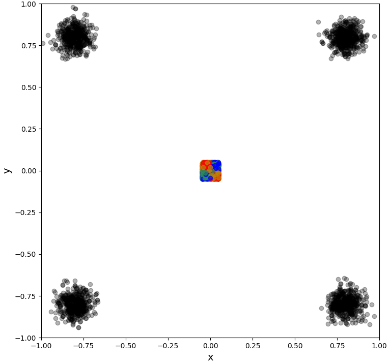
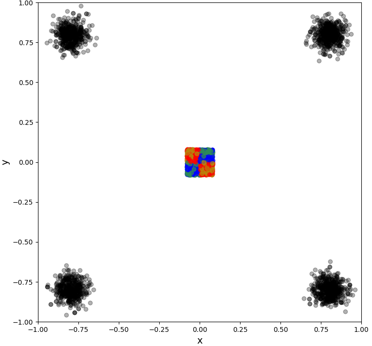
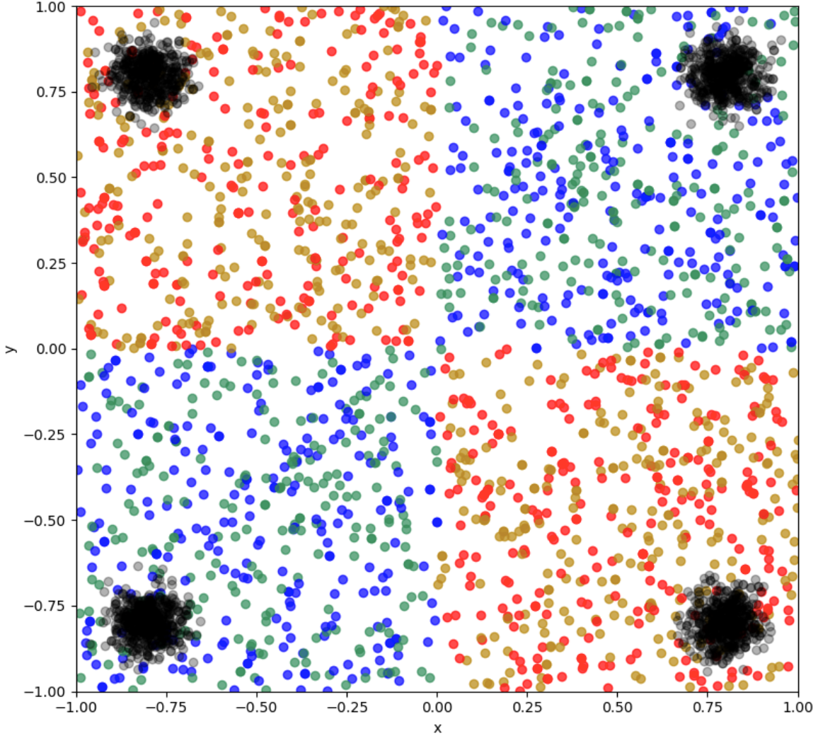
The training dataset for the 2D Multimodal Contextual Bandit Environment, $D=\{(s_{i},a_{i})\}^{n}_{i=1}$, consists of $n=10000$ state-action tuples with horizon $H=1$. To examine the policy in OOD states, the states generated for training are sampled from the uniform distribution $s_{train}\sim Uniform([-0.05,0.05]\times[-0.05,0.05])$ in Fig. 1(a), and $s_{train}\sim Uniform([-0.08,0.08]\times[-0.08,0.08])$ in Fig. 1(b). The states used for the evaluation are sampled from the uniform distribution of $s_{test}\sim Uniform([-1,1]\times[-1,1])$. Ground truth for OOD state generalization corresponding to the training datasets in Fig. 1(a) and (b) is illustrated in Fig. 1(c). The black points in Fig. 2(a) show the x and y-coordinates of the actions in the dataset, constituting two pairs of clusters located close to the diagonal edges of the 2D plane. Similarly, the black points in Fig. 2(a) and (b) show the x and y-coordinates of the actions generated by the SRDP and BC-Diffusion policies, respectively. To distinguish which states are mapped to which quadrants the actions reside in, we illustrate states in four different colors. More specifically, if a state generates an action in the first, second, third, and fourth quadrants, the state is colored red, green, dark yellow, and blue, respectively. Therefore, visually distinguishable quadrants with respective coloring in Fig. 2(a) (SRDP) indicate that the reverse diffusion process can generate actions accurately for OOD states. In contrast, Fig. 2(b) shows that BC-Diffusion memorizes actions without using state information. Subsequently, results in Fig. 2 show that the representation learning with state reconstruction loss promotes finding expert skills in multimodal data, achieving faster convergence. Although a larger portion of the state space is not included in the training set distribution ( $s_{train}\sim Uniform([-0.05,0.05]\times[-0.05,0.05])$) in Fig. 2, SRDP can generalize well to OOD states and learn at least one of the two expert behaviors. Conversely, BC-Diffusion finds the action distribution of the dataset, yet it cannot assign the correct action distribution for the given state. Hence, we observe that the state space is not partitioned correctly.

Figure 3: Top to bottom Row: SRDP (proposed model), BC-Diffusion [10], BC-CVAE [35], BC-MLE[37], BC-MMD [14]. Figures show the evaluations of the diffusion policies from left to right, where the number of training iterations increases incrementally by 4000. SRDP is trained with state reconstruction loss weight $\lambda=0.5$. Training dataset is constructed from $s_{train}\sim Uniform([-0.08,0.08]\times[-0.08,0.08]$)

In the next set of experiments, the training dataset includes ($s_{train},a_{train}$) tuples where $s_{train}\sim Uniform([-0.08,0.08]\times[-0.08,0.08]$). The comparison results with this setting show that only SRDP can represent multimodal expert distributions and partition the state space into visibly clear quadrants at earlier iterations, improving training stability and reducing computation costs. The last three rows in Fig. 3 show the results for BC-CVAE [35]), BC-MLE[37]), BC-MMD [14] which were used in Diffusion-QL 2D bandit experiments [10]. BC-CVAE, the policy model used in [35], represents the policy by a conditional variational encoder (CVAE) trained with the evidence lower bound $\displaystyle\mathbb{E}_{(\boldsymbol{s},\boldsymbol{a})\sim\mathcal{D}}\left[\mathbb{E}_{\boldsymbol{z}\sim q(\cdot\mid\boldsymbol{s},\boldsymbol{a})}[\log p(\boldsymbol{a}\mid\boldsymbol{s},\boldsymbol{z})]-\operatorname{KL}(q(\boldsymbol{z}\mid\boldsymbol{s},\boldsymbol{a})\|p(\boldsymbol{z}))\right]$ . BC-MLE [37] uses a Multivariate Gaussian to model the policy where a diagonal matrix represents the covariance. Finally, BC-MMD [14] uses a CVAE that learns the behavior policy to constrain a Gaussian policy. Our experiments show that although the bottleneck layer used in BC-CVAE increases the performance, the proposed model, SRDP, which uses state reconstruction loss, yields far better performance with faster convergence. Consistent with the experiments in Fig. 2, BC-Diffusion only learns the action distributions in the dataset, excluding the state information in OOD states. Hence, SRDP is the only method that can represent both expert modalities in this setting with the fastest convergence.

(a) Half-cheetah

(b) Hopper

(c) Walker2d

Figure 4: D4RL Gym-MuJoCo Environments

Figure 5: D4RL AntMaze Environments with three different layouts: (a) Antmaze-umaze-v0, (b) Antmaze-medium-v0, (c) Antmaze-large-v0

V-B D4RL Environment

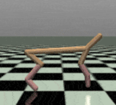
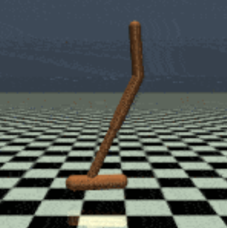
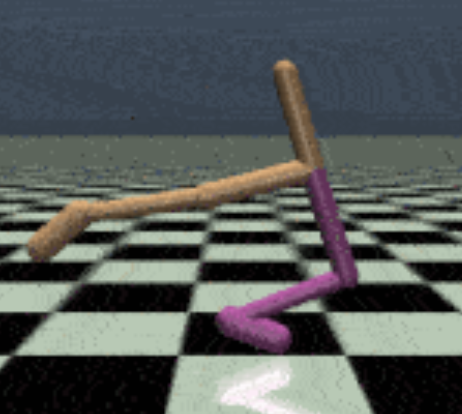
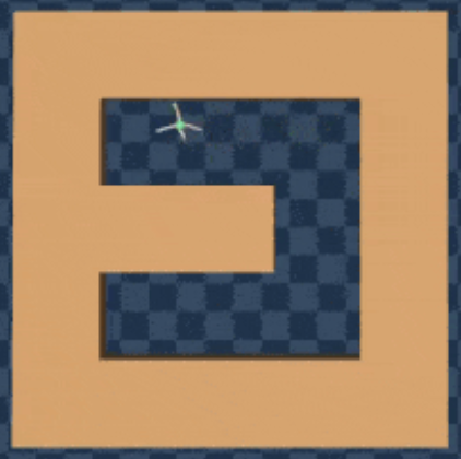
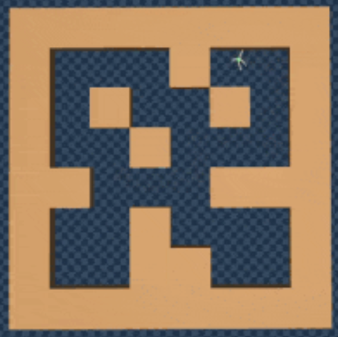
D4RL environments, comprising extensive robotics datasets, have been widely used as a benchmark for offline RL algorithms. In this section, we evaluate our method on AntMaze and Gym-MuJoCo robotics datasets. In AntMaze environments, the objective of an 8-DoF quadruped ant robot is to navigate to a 2D goal location in various mazes. Similarly, Gym-MuJoCo datasets are generated with half-cheetah, hopper, and walker2d robots performing forward locomotion. Since offline RL differs from imitation learning, each dataset in Table includes various amounts of suboptimal data. For these experiments, we follow the details of the online implementation used in Diffusion-QL, where they assume that the policies can be evaluated at fixed intervals with few online interactions. This is a form of early stopping in RL introduced in [39] where the hyperparameter, the number of training epochs, is tuned for Diffusion-QL and the proposed model, SRDP. We report the average normalized scores of undiscounted returns for SRDP and Diffusion-QL in Table 1, where 100 corresponds to expert-level behavior. The normalized scores for Diffusion-QL are from [10].

TABLE I: Comparison of SRDP with the Diffusion-QL baseline.

$\mathbf{AntMaze}$	$\mathbf{Diffusion}$-$\mathbf{QL}$	$\mathbf{SRDP(ours)}$
antmaze-umaze-v0	96.0	$\boldsymbol{96.4}\pm 1.5$
antmaze-umaze-diverse-v0	84.0	$\boldsymbol{89.8}\pm 5.1$
antmaze-medium-play-v0	$\boldsymbol{79.8}$	$78.4\pm 8.1$
antmaze-medium-diverse-v0	82.0	$\boldsymbol{90.6}\pm 6.0$
antmaze-large-play-v0	49.0	$\boldsymbol{63.0}\pm 8.0$
antmaze-large-diverse-v0	61.7	$\boldsymbol{62.6}\pm 3.5$
$\mathbf{Average}$	75.4	$\boldsymbol{80.1}$
$\mathbf{Gym}$	$\mathbf{Diffusion}$-$\mathbf{QL}$	$\mathbf{SRDP(ours)}$
halfcheetah-medium-v2	51.5	$\boldsymbol{51.9}\pm 1.5$
hopper-medium-v2	96.6	$\boldsymbol{96.8}\pm 3.1$
walker2d-medium-v2	87.3	$\boldsymbol{88.1}\pm 0.5$
halfcheetah-medium-replay-v2	$\boldsymbol{48.3}$	$48.1\pm 0.3$
hopper-medium-replay-v2	102.0	$\boldsymbol{102.1}\pm 0.1$
walker2d-medium-replay-v2	98.0	$\boldsymbol{98.1}\pm 1.2$
halfcheetah-medium-expert-v2	97.2	$\boldsymbol{97.5}\pm 0.1$
hopper-medium-expert-v2	112.3	$\boldsymbol{112.6}\pm 0.4$
walker2d-medium-expert-v2	$\boldsymbol{111.2}$	$111.1\pm 0.4$
$\mathbf{Average}$	89.3	$\boldsymbol{89.6}$

Antmaze datasets are generated following nonmarkovian and suboptimal policies, sparse rewards, and multitask data design procedures [1]. Fig. 5 shows the AntMaze environments where each maze layout, umaze, medium, and large, has different levels, such as play and diverse. The performance scores across five random seeds in Table 1 demonstrate that the proposed model, SRDP policies, are superior for all cases except antmaze-medium-play-v0. Out-of-distribution data generalization is beneficial in multitask settings; hence SRDP policies can enhance performance significantly in Antmaze datasets.

Gym-MuJoCo environments, comprising continuous control tasks in MuJoCo [40], has been commonly used in deep RL [1, 41, 37, 42, 43]. In D4RL, datasets are collected using the online RL interaction data of a Soft Actor-Critic (SAC) [42, 1]. To evaluate an offline-RL algorithm in narrow data distribution and suboptimal behavior policy settings, “medium”, “medium-replay”, and “medium-expert” datasets are generated. Medium datasets are generated by collecting the rollouts from a medium-performing policy whereas medium-replay datasets are generated by keeping a replay buffer of rollouts until the RL policy reaches a medium-level performance. Medium-expert datasets, on the other hand, include expert trajectories by fifty percent in addition to medium-level rollouts. Gym-MuJoCo environments are not explicitly designed to benchmark OOD states, yet results presented in Table 1 show that our proposed model, SRDP, performs better to Diffusion QL across five random seeds [10].

VI Conclusion

In this work, we propose SRDP for out-of-distribution generalization in offline RL, a representation learning-based method built on top of the recent class of diffusion policies introduced by [10]. To show the multiple skills learned by the model when evaluated in OOD states, we designed a simple 2D Multimodal Contextual Bandit environment. We thoroughly discuss and illustrate how SRDP uses guidance from the state reconstruction loss to learn more descriptive features from 2D Multimodal Contextual Bandit datasets. Our results indicate that, compared to prior work, SRDP can represent multimodal policies, partition the state space more accurately, and converge faster. We empirically show that SRDP can learn superior models compared to previous work in Antmaze and Gym-MuJoCo environments in D4RL benchmarks [1] with a wide variety of levels (umaze, umaze-diverse, medium-diverse, large-play, large-diverse) and agents (ant, half cheetah, hopper, walker2d). For future work, we intend to evaluate our model on more challenging offline RL tasks designed for OOD generalization.

APPENDIX

VI-A 2D-Contextual Multimodal Bandit Experimental Details and Architectural Analysis

(a) BC-Diffusion with hidden layer size M=32.

Figure 6: Training dataset is constructed from $s_{train}\sim Uniform([-0.05,0.05]\times[-0.05,0.05]$). The number of training iterations in each column increases incrementally from left to right by 2000, starting from 32000, corresponding to the same number of epochs in Fig.2.

Fig. 6 and 7 show the evaluations of BC-Diffusion, BC-CVAE, BC-MLE, and BC-MMD with increased model capacity for a training dataset constructed from $s_{train}\sim Uniform([-0.05,0.05]\times[-0.05,0.05]$) and $s_{train}\sim Uniform([-0.08,0.08]\times[-0.08,0.08]$) respectively.

(a) BC-Diffusion with hidden layer size M=32

(b) Top to bottom: BC-CVAE, BC-MLE, and BC-MMD with hidden layer size M=32

Figure 7: Evaluations of the diffusion policies from left to right where the number of training iterations increases incrementally by 4000, the last column referring to the $20000^{th}$ iteration, corresponding to the same number of epochs in Fig.3. Training dataset is constructed from $s_{train}\sim Uniform([-0.08,0.08]\times[-0.08,0.08]$.

We use Bottleneck Dual Head BDH2 architecture with hidden layer sizes $(32^{shared},16^{shared},32)$ and state reconstruction loss weight $\lambda=0.5$ for SRDP in the experiments shown in Fig. 3; hence, we provide an additional comparative analysis with algorithms with increased model capacity. In addition, we omitted the figures for layer sizes 8 and 64 because all models performed poorly. All hidden layers have the same size 16 for SRDP and BC-Diffusion in Fig. 2. SRDP is trained with state reconstruction loss weight $\lambda=1.25$ and a dual head architecture with hidden layer sizes $(16^{shared},16^{shared},16^{shared})$ for ablation in Fig. 2.

References

- [1] J. Fu, A. Kumar, O. Nachum, G. Tucker, and S. Levine, “D4rl: Datasets for deep data-driven reinforcement learning,” arXiv preprint arXiv:2004.07219, 2020.
- [2] A. Radford, K. Narasimhan, T. Salimans, and I. Sutskever, “Improving language understanding by generative pre-training,” 2018.
- [3] A. Radford, J. Wu, R. Child, D. Luan, D. Amodei, and I. Sutskever, “Language models are unsupervised multitask learners,” 2019.
- [4] T. Brown, B. Mann, N. Ryder, M. Subbiah, J. D. Kaplan, P. Dhariwal, A. Neelakantan, P. Shyam, G. Sastry, A. Askell, et al., “Language models are few-shot learners,” Advances in neural information processing systems, vol. 33, pp. 1877–1901, 2020.
- [5] L. Ouyang, J. Wu, X. Jiang, D. Almeida, C. L. Wainwright, P. Mishkin, C. Zhang, S. Agarwal, K. Slama, A. Ray, J. Schulman, J. Hilton, F. Kelton, L. E. Miller, M. Simens, A. Askell, P. Welinder, P. F. Christiano, J. Leike, and R. J. Lowe, “Training language models to follow instructions with human feedback,” ArXiv, vol. abs/2203.02155, 2022.
- [6] Y. Liu, T. Han, S. Ma, J. Zhang, Y. Yang, J. Tian, H. He, A. Li, M. He, Z. Liu, et al., “Summary of chatgpt/gpt-4 research and perspective towards the future of large language models,” arXiv preprint arXiv:2304.01852, 2023.
- [7] X. Fang, Q. Zhang, Y. Gao, and D. Zhao, “Offline reinforcement learning for autonomous driving with real world driving data,” in 2022 IEEE 25th International Conference on Intelligent Transportation Systems (ITSC), 2022, pp. 3417–3422.
- [8] S. Levine, A. Kumar, G. Tucker, and J. Fu, “Offline reinforcement learning: Tutorial, review, and perspectives on open problems,” CoRR, vol. abs/2005.01643, 2020. [Online]. Available: https://arxiv.org/abs/2005.01643
- [9] J. Li, C. Tang, M. Tomizuka, and W. Zhan, “Dealing with the unknown: Pessimistic offline reinforcement learning,” in 5th Annual Conference on Robot Learning, 2021. [Online]. Available: https://openreview.net/forum?id=ftOqDUeLPn3
- [10] Z. Wang, J. J. Hunt, and M. Zhou, “Diffusion policies as an expressive policy class for offline reinforcement learning,” in The Eleventh International Conference on Learning Representations, 2023. [Online]. Available: https://openreview.net/forum?id=AHvFDPi-FA
- [11] M. Janner, Y. Du, J. B. Tenenbaum, and S. Levine, “Planning with diffusion for flexible behavior synthesis,” in International Conference on Machine Learning, 2022.
- [12] T. Denouden, R. Salay, K. Czarnecki, V. Abdelzad, B. Phan, and S. Vernekar, “Improving reconstruction autoencoder out-of-distribution detection with mahalanobis distance,” arXiv preprint arXiv:1812.02765, 2018.
- [13] U. Mutlu and E. Alpaydın, “Training bidirectional generative adversarial networks with hints,” Pattern Recognition, vol. 103, p. 107320, 2020. [Online]. Available: https://www.sciencedirect.com/science/article/pii/S0031320320301230
- [14] A. Kumar, J. Fu, G. Tucker, and S. Levine, “Stabilizing off-policy q-learning via bootstrapping error reduction,” CoRR, vol. abs/1906.00949, 2019. [Online]. Available: http://arxiv.org/abs/1906.00949
- [15] Y. Wu, G. Tucker, and O. Nachum, “Behavior regularized offline reinforcement learning,” CoRR, vol. abs/1911.11361, 2019. [Online]. Available: http://arxiv.org/abs/1911.11361
- [16] A. Nair, M. Dalal, A. Gupta, and S. Levine, “Accelerating online reinforcement learning with offline datasets,” CoRR, vol. abs/2006.09359, 2020. [Online]. Available: https://arxiv.org/abs/2006.09359
- [17] I. Kostrikov, A. Nair, and S. Levine, “Offline reinforcement learning with implicit q-learning,” CoRR, vol. abs/2110.06169, 2021. [Online]. Available: https://arxiv.org/abs/2110.06169
- [18] A. Kumar, A. Zhou, G. Tucker, and S. Levine, “Conservative q-learning for offline reinforcement learning,” CoRR, vol. abs/2006.04779, 2020. [Online]. Available: https://arxiv.org/abs/2006.04779
- [19] S. Zhang, B. Liu, and S. Whiteson, “GradientDICE: Rethinking generalized offline estimation of stationary values,” in Proceedings of the 37th International Conference on Machine Learning, ser. Proceedings of Machine Learning Research, H. D. III and A. Singh, Eds., vol. 119. PMLR, 13–18 Jul 2020, pp. 11 194–11 203. [Online]. Available: https://proceedings.mlr.press/v119/zhang20r.html
- [20] N. Jiang and L. Li, “Doubly robust off-policy evaluation for reinforcement learning,” CoRR, vol. abs/1511.03722, 2015. [Online]. Available: http://arxiv.org/abs/1511.03722
- [21] T. Yu, G. Thomas, L. Yu, S. Ermon, J. Zou, S. Levine, C. Finn, and T. Ma, “MOPO: model-based offline policy optimization,” CoRR, vol. abs/2005.13239, 2020. [Online]. Available: https://arxiv.org/abs/2005.13239
- [22] T. Yu, A. Kumar, R. Rafailov, A. Rajeswaran, S. Levine, and C. Finn, “COMBO: conservative offline model-based policy optimization,” CoRR, vol. abs/2102.08363, 2021. [Online]. Available: https://arxiv.org/abs/2102.08363
- [23] M. Janner, Q. Li, and S. Levine, “Reinforcement learning as one big sequence modeling problem,” CoRR, vol. abs/2106.02039, 2021. [Online]. Available: https://arxiv.org/abs/2106.02039
- [24] L. Chen, K. Lu, A. Rajeswaran, K. Lee, A. Grover, M. Laskin, P. Abbeel, A. Srinivas, and I. Mordatch, “Decision transformer: Reinforcement learning via sequence modeling,” CoRR, vol. abs/2106.01345, 2021. [Online]. Available: https://arxiv.org/abs/2106.01345
- [25] J. Sohl-Dickstein, E. A. Weiss, N. Maheswaranathan, and S. Ganguli, “Deep unsupervised learning using nonequilibrium thermodynamics,” CoRR, vol. abs/1503.03585, 2015. [Online]. Available: http://arxiv.org/abs/1503.03585
- [26] J. Yue, L. Fang, S. Xia, Y. Deng, and J. Ma, “Dif-fusion: Towards high color fidelity in infrared and visible image fusion with diffusion models,” CoRR, vol. abs/2301.08072, 2023. [Online]. Available: https://doi.org/10.48550/arXiv.2301.08072
- [27] M. Wei, Y. Shen, Y. Wang, H. Xie, and F. L. Wang, “Raindiffusion: When unsupervised learning meets diffusion models for real-world image deraining,” CoRR, vol. abs/2301.09430, 2023. [Online]. Available: https://doi.org/10.48550/arXiv.2301.09430
- [28] D. Eschweiler and J. Stegmaier, “Denoising diffusion probabilistic models for generation of realistic fully-annotated microscopy image data sets,” CoRR, vol. abs/2301.10227, 2023. [Online]. Available: https://doi.org/10.48550/arXiv.2301.10227
- [29] F. Bao, C. Li, Y. Cao, and J. Zhu, “All are worth words: a vit backbone for score-based diffusion models,” CoRR, vol. abs/2209.12152, 2022. [Online]. Available: https://doi.org/10.48550/arXiv.2209.12152
- [30] J. C. White and R. Cotterell, “Schrödinger’s bat: Diffusion models sometimes generate polysemous words in superposition,” CoRR, vol. abs/2211.13095, 2022. [Online]. Available: https://doi.org/10.48550/arXiv.2211.13095
- [31] J. Ho, A. Jain, and P. Abbeel, “Denoising diffusion probabilistic models,” in Advances in Neural Information Processing Systems, H. Larochelle, M. Ranzato, R. Hadsell, M. Balcan, and H. Lin, Eds., vol. 33. Curran Associates, Inc., 2020, pp. 6840–6851. [Online]. Available: https://proceedings.neurips.cc/paper/2020/file/4c5bcfec8584af0d967f1ab10179ca4b-Paper.pdf
- [32] L. Yang, Z. Zhang, Y. Song, S. Hong, R. Xu, Y. Zhao, Y. Shao, W. Zhang, B. Cui, and M.-H. Yang, “Diffusion models: A comprehensive survey of methods and applications,” 2022. [Online]. Available: https://arxiv.org/abs/2209.00796
- [33] R. S. Sutton and A. G. Barto, Reinforcement learning: An introduction. MIT Press, 2018.
- [34] H. Hasselt, “Double q-learning,” in Advances in Neural Information Processing Systems, J. Lafferty, C. Williams, J. Shawe-Taylor, R. Zemel, and A. Culotta, Eds., vol. 23. Curran Associates, Inc., 2010. [Online]. Available: https://proceedings.neurips.cc/paper/2010/file/091d584fced301b442654dd8c23b3fc9-Paper.pdf
- [35] S. Fujimoto, D. Meger, and D. Precup, “Off-policy deep reinforcement learning without exploration,” in International Conference on Machine Learning, 2018.
- [36] T. P. Lillicrap, J. J. Hunt, A. Pritzel, N. Heess, T. Erez, Y. Tassa, D. Silver, and D. Wierstra, “Continuous control with deep reinforcement learning,” in 4th International Conference on Learning Representations, ICLR 2016, San Juan, Puerto Rico, May 2-4, 2016, Conference Track Proceedings, Y. Bengio and Y. LeCun, Eds., 2016. [Online]. Available: http://arxiv.org/abs/1509.02971
- [37] S. Fujimoto and S. Gu, “A minimalist approach to offline reinforcement learning,” in Advances in Neural Information Processing Systems, A. Beygelzimer, Y. Dauphin, P. Liang, and J. W. Vaughan, Eds., 2021. [Online]. Available: https://openreview.net/forum?id=Q32U7dzWXpc
- [38] Z. Wang, “Diffusion-policies-for-offline-rl,” 2022, https://github.com/Zhendong-Wang/Diffusion-Policies-for-Offline-RL, Accessed in 2023.
- [39] S. E. Ada, E. Ugur, and H. L. Akin, “Generalization in transfer learning: robust control of robot locomotion,” Robotica, vol. 40, no. 11, p. 3811–3836, 2022.
- [40] E. Todorov, T. Erez, and Y. Tassa, “Mujoco: A physics engine for model-based control,” in Intelligent Robots and Systems (IROS), 2012 IEEE/RSJ International Conference on. IEEE, 2012, pp. 5026–5033.
- [41] L. Chen, K. Lu, A. Rajeswaran, K. Lee, A. Grover, M. Laskin, P. Abbeel, A. Srinivas, and I. Mordatch, “Decision transformer: Reinforcement learning via sequence modeling,” arXiv preprint arXiv:2106.01345, 2021.
- [42] T. Haarnoja, A. Zhou, P. Abbeel, and S. Levine, “Soft actor-critic: Off-policy maximum entropy deep reinforcement learning with a stochastic actor,” arXiv preprint arXiv:1801.01290, 2018.
- [43] D. Brandfonbrener, W. F. Whitney, R. Ranganath, and J. Bruna, “Offline RL without off-policy evaluation,” in Advances in Neural Information Processing Systems, A. Beygelzimer, Y. Dauphin, P. Liang, and J. W. Vaughan, Eds., 2021. [Online]. Available: https://openreview.net/forum?id=LU687itn08w