Quark/Gluon Discrimination and Top Tagging with Dual Attention Transformer

Abstract

Jet tagging is a crucial classification task in high energy physics. Recently the performance of jet tagging has been significantly improved by the application of deep learning techniques. In this work, we propose Particle Dual Attention Transformer for jet tagging, a new transformer architecture which captures both global information and local information simultaneously. Based on the point cloud representation, we introduce the Channel Attention module to the point cloud transformer and incorporates both the pairwise particle interactions and the pairwise jet feature interactions in the attention mechanism. We demonstrate the effectiveness of the P-DAT architecture in classic top tagging and quark-gluon discrimination tasks, achieving competitive performance compared to other benchmark strategies.

1 Introduction

In high-energy physics experiments, tagging jets, which are collimated sprays of particles produced from high-energy collisions, is a crucial task for discovering new physics beyond the Standard Model. Jet tagging involves distinguishing boosted heavy particle jets from those of QCD initiated quark/gluon jets. Since jets initiated by different particles exhibit different characteristics, two key issues arise: how to represent a jet and how to analyze its representation. Conventionally, jet tagging has been performed using hand-crafted jet substructure variables based on physics motivation. Nevertheless, these methods can often fall short in capturing intricate patterns and correlations present in the raw data.

Over the past decade, deep learning approaches have been extensively adopted to enhance the jet tagging performance[20]. Various jet representations have been proposed, including image-based representation using Convolutional Neural Network (CNN)[8, 11, 32, 2, 22, 18, 26, 21], sequence-based representation with Recurrent Neural Network[10, 1], tree-based representation with Recursive Neural Network[7, 24] and graph-based representation with Graph Neural Network (GNN)[17, 25, 3, 4, 15, 33]. More recently, One representation approach that has gained significant attention is to view the set of constituent particles inside a jet as points in a point cloud. Point clouds are used to represent a set of objects in an unordered manner, described in a defined space, and are commonly utilized in various fields such as self-driving vehicles, robotics, and augmented reality. By adopting this approach, each jet can be interpreted as a particle cloud, which treats a jet as a permutation-invariant set of particles, allowing us to extract meaningful information with deep learning method. Based on the particle cloud representation, several deep learning architectures have been proposed, including Deep Set Framework[19], ABCNet[27], LorentzNet[15] and ParticleNet[30]. The Deep Set Framework provides a comprehensive explanation of how to parametrize permutation invariant functions for inputs with variable lengths, taking into consideration both infrared and collinear safety. Furthermore, it offers valuable insights into the nature of the learned features by neural networks. ParticleNet adapts the Dynamic Graph CNN architecture[37], while ABCNet takes advantage of attention mechanisms to enhance the local feature extraction. The LorentzNet focused more on incorporating inductive biases derived from physics principles into the architecture design, utilizing an efficient Minkowski dot product attention mechanism. All of these architectures realize substantial performance improvement on top tagging and quark/gluon discrimination benchmarks.

Over the past few years, attention mechanisms have become as a powerful tool for capturing intricate patterns in sequential and spatial data. The Transformer architecture[35], which leverages attention mechanisms, has been highly successful in natural language processing and computer vision tasks such as image recognition. Notably, the Vision Transformer (ViT)[13, 38], initially designed for computer vision tasks, has demonstrated state-of-the-art performance on various image classification benchmarks. However, when dealing with point cloud representation, which inherently lack a specific order, modifications to the original Transformer structure are required to establish a self-attention operation that is invariant to input permutations. To address these issues, a recent approach called Point Cloud Transformer (PCT)[16, 28] was proposed, which entails passing input points through a feature extractor to create a high-dimensional representation of particle features. The transformed data is then passed through a self-attention module that introduces attention coefficients for each pair of particles. To evaluate PCT’s effectiveness in the context of a high-energy physics task, specifically jet-tagging, PCT was compared with other benchmark implementations using three different public datasets. PCT shares a similar concept with the ABCNet’s attention mechanism, employing a self-attention layer to capture the importance of relationships between all particles in the dataset. Another notable approach is the Particle Transformer[31], which incorporates pairwise particle interactions within the attention mechanism and obtains higher tagging performance than a plain Transformer and surpasses the previous state-of-the-art, ParticleNet, by a large margin.

In recent studies, the Dual Attention Vision Transformer (DaViT)[12] has exhibited promising results for image classification. The DaViT introduces the dual attention mechanism, comprising spatial window attention and channel group attention, enabling the effective capture of both global and local features in images. These two self-attentions are demonstrated to complement each other. In this paper, we introduce the Channel Attention module to the Point Cloud Transformer and incorporate the pairwise particle interaction and the pairwise jet feature interaction to build a new network structure, called P-DAT. On the one hand, the Channel Attention module can grasp comprehensive spatial interactions and representations by taking into account all spatial locations while computing attention scores between channels. In this way, the P-DAT can combine both the local information and global information of the jet representation for jet tagging. On the other hand, the pairwise interaction features designed from physics principles can modify the dot-product attention weights, thus increasing the expressiveness of the attention mechanism. We evaluate the performance of P-DAT on top tagging and quark/gluon discrimination tasks and compare its performance against other baseline models. Our analysis demonstrates the effectiveness of P-DAT in jet tagging and highlights its potential for future applications in high-energy physics experiments.

This article is organized as follows. In Section 2, we introduce the Particle Dual Attention Transformer for jet tagging and describe the key features of the model architecture. We also provide details of the training and validation process. In Section 3, we present and discuss the numerical results obtained for top tagging task and quark/gluon discrimination task, respectively. Finally, our conclusions are presented in Section 4.

2 Model Architecture

The focus of this paper is to introduce the Particle Dual Attention Transformer (P-DAT), which serves as a new benchmark approach for jet tagging. Based on the point cloud representation, we regard each constituent particle as a point in the $\eta-\phi$ space and the whole jet as a point cloud. The whole model architecture is presented in Figure.1.

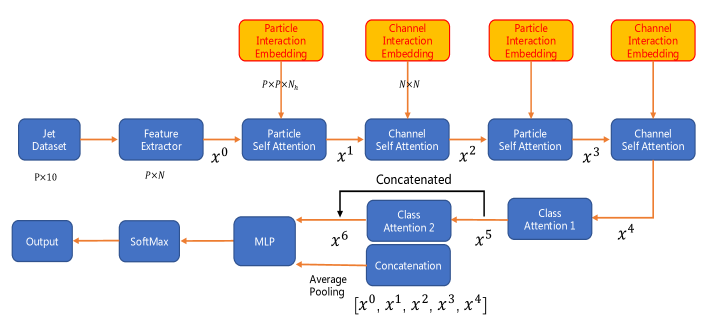
Figure 1: Illustration of the whole model architecture.

The P-DAT architecture is composed of 5 main building blocks, namely the feature extractor, the particle self attention layers, the channel self attention layers, the class attention layers and the MLP. In order to process a jet of P particles, the P-DAT requires three inputs: the jet dataset, the particle interaction matrix and the jet feature interaction matrix derived from the kinetic information of each particle inside the jet. First of all, the feature extractor is employed to transform the input jet dataset from $P\times 10$ to a higher dimensional representation $P\times N$. As illustrated in Fig.2(left), the feature extractor block contains two parts. The first part incorporates an EdgeConv operation[36] followed by 3 two-dimensional convolutional (Conv2D) layers and an average pooling operation across all neighbors of each particle. The EdgeConv operation adopts a k-nearest neighbors approach with $k=20$ to define a vicinity for each particle inside the jet based on $\Delta R=\sqrt{\Delta\eta^{2}+\Delta\phi^{2}}$ in the $\eta-\phi$ space to extract the local information for each particle. To ensure the permutation invariance among particles, all convolutional layers are implemented with stride and kernel size of 1 and are followed by a batch normalization operation and GeLU activation function. The second part of the feature extractor consists of 3-layer MLP with $(128,128,128)$ nodes each layer with GELU nonlinearity to handle the negative inputs. BN and LN operations are used for normalization between layers. Finally, the output from these two parts are concatenated to obtain the final output. This approach enables the extraction of input particle embeddings through both linear projection and local neighborhood mapping. Furthermore, we introduce a particle interaction matrix and a channel interaction matrix, both of which are designed based on physics principles and incorporated into the self attention module. For the particle interaction matrix, we use a 3-layer 2D convolution with (32,16,8) channels with stride and kernel size of 1 to map the particle interaction matrix to a new embedding $P\times P\times N_{h}$, where $N_{h}$ is the number of heads in the particle self attention module which will be explained later. As for the channel interaction matrix, an upsampling operation and a 3-layer 2D convolution are applied to map the channel interaction matrix to a higher dimensional representation $N\times N$, with $N$ the input particle embedding dimension.

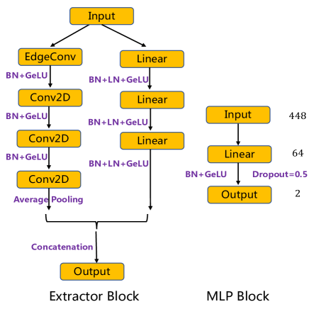
Figure 2: Illustration of the Feature extractor block and the MLP block.

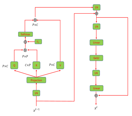
Figure 3: Illustration of the Particle Multi-head Attention Block.

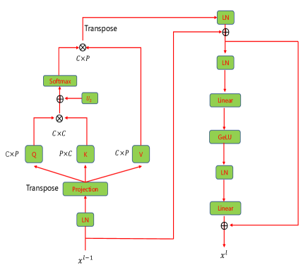
Figure 4: Illustration of the Channel Attention Block.

The second primary building block is the particle self-attention block, which aims to establish the relationship between all particles within the jet using an attention mechanism. As presented in Fig.3, three matrices, which are called query (Q), key (K), and value (V), are built from linear transformations of the original inputs. Attention weights are computed by matrix multiplication between Q and K, representing the matching between them. Similar to the Particle Transformer work[31], we incorporate the particle interaction matrix $U_{1}$ as a bias term to enhance the scaled dot-product attention. This incorporation of particle interaction features, designed from physics principles, modifies the dot-product attention weights, thereby enhancing the expressiveness of the attention mechanism. The same $U_{1}$ is shared across the two particle attention blocks. After normalization, these attention weights reflect the weighted importance between each pair of particles. The self-attention is then obtained by the weighted elements of V, which result from multiplying the attention weights and the value matrix. It is important to note that $P$ represents the number of particles, and $N$ denotes the total number of features. The attention weights are computed as:

$$\mathcal{A}(\mathbf{Q},\mathbf{K},\mathbf{V}) =\mathrm{Concat}(\mbox{head}_{1},\ldots,\mbox{head}_{N_{h}})$$

$$\text{where}~{}~{}\mbox{head}_{i} =\mathrm{Attention}(\mathbf{Q}_{i},\mathbf{K}_{i},\mathbf{V}_{i})$$

$$=\mathrm{softmax}\left[\frac{\mathbf{Q}_{i}(\mathbf{K}_{i})^{\mathrm{T}}}{\sqrt{C_{h}}}+\mathbf{U_{1}}\right]\mathbf{V}_{i}$$ (1)

where $\mathbf{Q}_{i}=\mathbf{X}_{i}\mathbf{W}_{i}^{Q}$, $\mathbf{K}_{i}=\mathbf{X}_{i}\mathbf{W}_{i}^{K}$, and $\mathbf{V}_{i}=\mathbf{X}_{i}\mathbf{W}_{i}^{V}$ are $\mathbb{R}^{P\times N_{h}}$ dimensional visual features with $N_{h}$ heads, $\mathbf{X}_{i}$ denotes the $i_{th}$ head of the input feature and $\mathbf{W}_{i}$ denotes the projection weights of the $i_{th}$ head for $\mathbf{Q},\mathbf{K},\mathbf{V}$, and $N=C_{h}*N_{h}$. The particle attention block incorporates a LayerNorm (LN) layer both before and after the multi-head attention module. A two-layer MLP, with LN preceding each linear layer and GELU nonlinearity in between, follows the multi-head attention module. Residual connections are applied after the multi-head attention module and the two-layer MLP. In our study, we set $N_{h}=8$ and $N=64$.

The third main building block is the channel self-attention block, as shown in Fig.4. Unlike the particle self-attention block, this block applies attention mechanisms to the jet features, enabling interactions among the channels. To capture global information in the particle dimension, we set the number of heads to 1, where each transposed token represents global information. Consequently, the channel tokens interact with global information across all channels. This global channel attention mechanism is defined as follows:

$$\mathcal{A}(\mathbf{Q}_{i},\mathbf{K}_{i},\mathbf{V}_{i}) =\mathrm{softmax}\left[\frac{\mathbf{Q}_{i}^{\mathrm{T}}\mathbf{K}_{i}}{\sqrt{C}}+\mathbf{U_{2}}\right]\mathbf{V}_{i}^{T}$$ (2)

where $\mathbf{Q}_{i},\mathbf{K}_{i},\mathbf{V}_{i}\in\mathbb{R}^{C\times P}$ are channel-wise jet-level queries, keys, and values. Note that although we transpose the tokens in the channel attention block, the projection layers $\mathbf{W}$ and the scaling factor $\frac{1}{\sqrt{C}}$ are computed along the channel dimension, rather than the particle dimension. Similar as the particle self-attention block, we incorporate the channel interaction matrix $U_{2}$ as a bias term to enhance the scaled dot-product attention. This incorporation of jet channel interaction features, designed based on physics principles, modifies the dot-product attention weights, thereby enhancing the expressiveness of the attention mechanism. The same $U_{2}$ matrix is shared across the two channel attention blocks. After normalization, the attention weights indicate the weighted importance of each pair of jet features. The self-attention mechanism produces the weighted elements of V, obtained by multiplying the attention weights and the value matrix. Additionally, the channel attention block includes a LayerNorm (LN) layer before and after the attention module, followed by a two-layer MLP. Each linear layer is preceded by an LN layer, and a GELU nonlinearity is applied between them. Residual connections are added after the channel attention module and the two-layer MLP.

The fourth main building block is the class attention block, which differs from the particle self-attention block by computing attention between a global class token and all particles using the standard Multi-Head Attention (MHA) mechanism. This class channel attention mechanism is defined as follows:

$$\begin{split}Q&=W_{q}x_{\text{class}}+b_{q},\\ K&=W_{q}z+b_{k},\\ V&=W_{q}z+b_{v},\\ z&=[x_{\text{class}},x^{L}]\end{split}$$ (3)

where $z=[x_{class},x^{L}]$ represents the concatenation of the class token and the particle embedding after the last particle attention block, denoted as $x_{L}$. In the first class attention block, the class token is obtained by performing max pooling on the output of the second channel attention block across all particles. In the second class attention block, the class token is obtained by performing average pooling on the output of the second channel attention block across all particles. Furthermore, the class attention block includes a LayerNorm (LN) layer before and after the attention module, followed by a two-layer MLP. Each linear layer is preceded by an LN layer, and a GELU nonlinearity is applied between them. Residual connections are added after the class attention module and the two-layer MLP.

The last main building block is a 3-layer MLP with (448, 64, 2) nodes, as shown in Fig.2(right). First, the outputs of the particle attention blocks and channel attention blocks are concatenated, followed by an average pooling operation across all particles. Subsequently, the outputs of the class attention blocks are concatenated. Finally, these two sets of outputs are concatenated and fed into the MLP. In addition, a batch normalization operation and the GeLU activation function are applied to the second layer, and a dropout rate of 0.5 is applied to the second layer. The last layer employs a softmax operation to produce the final classification scores.

In summary, the P-DAT are composed of one feature extractor, two particle attention blocks, two channel attention blocks, two class attention blocks and one MLP. The feature extractor’s output serves as the input for the first particle attention block. Subsequently, we alternate between the particle attention block and the channel attention block to capture both local fine-grained and global features. A dropout rate of 0.1 is applied to all particle attention blocks and channel attention blocks. As demonstrated in Ref.[12], these two blocks complement each other: the channel attention provides a global receptive field in the particle dimension, enabling the extraction of high-level global jet representations by dynamically fusing features across global channel tokens. On the other hand, the particle attention refines local representations by facilitating fine-grained interactions among all particles, thereby aiding in the modeling of global information in the channel attention. After the second channel attention block, two class attention blocks which take the max pooling and average pooling on the output of the second channel attention block as class token are applied to compute the attention between a global class token and all particles using the standard Multi-Head Attention (MHA) mechanism. Finally, the two sets of outputs are concatenated and fed into the MLP and the resulting representation is normalized using a softmax operation.

The model architecture is implemented in the PYTORCH deep learning framework with the CUDA platform. The training and evaluation steps are accelerated using a NVIDIA GeForce RTX 3070 GPU for acceleration. We adopt the binary cross-entropy as the loss function. To optimize the model parameters, we employ the AdamW optimizer[23] with an initial learning rate of 0.0004, which is determined based on the gradients calculated on a mini-batch of 64 training examples. In order to address the memory issue caused by huge input data, we implemented a strategy of continuously importing and deleting data during the training process. The network is trained up to 100 epochs, with the learning rate decreasing by a factor of 2 every 10 epochs to a minimal of $10^{-6}$. In addition, we employ the early-stopping technique to prevent over-fitting.

3 Jet Classification

The P-DAT architecture is designed to process input data consisting of particles inside the jets. To ensure consistency and facilitate meaningful comparisons, we first sorted the particles inside the jets by transverse momentum and a maximum of 100 particles per jet are employed. The input jet is truncated if the particle number inside the jet is more than 100 and the input jet is zero-padded up to the 100 if fewer than 100 particles are present. This selection of 100 particles is sufficient to cover the vast majority of jets contained within all datasets, ensuring comprehensive coverage. Each jet is characterized by the 4-momentum of its constituent particles. Based on this information, we reconstructed 10 features for each particle. Additionally, for the quark-gluon dataset, we included the Particle Identification (PID) information as the 11-th feature. These features are as follows:

$$\left\{\begin{aligned} \text{log $E$},\ \text{log $|p_{x}|$},\ \text{log $|p_{y}|$},\ \text{log $|p_{z}|$},\ \\ \text{log $p_{\text{T}}$},\ \frac{p_{\text{T}}}{p_{\text{TJ}}},\ \frac{E}{E_{J}},\ \Delta\eta\ \Delta\phi,\ \Delta R,\ \text{PID}\end{aligned}\right\}.$$ (4)

For the pairwise particle interaction matrix, based on Refs.[31, 14], we calculated the following 5 features for any pair of particles a and b with four-momentum $p_{a}$ and $p_{b}$ as the sum of all the particles’ four-momentum inside the particle a and particle b, respectively:

$$\begin{split}\Delta R&=\sqrt{(y_{a}-y_{b})^{2}+(\phi_{a}-\phi_{b})^{2}},\\ k_{\text{T}}&=\min(p_{\text{T},a},p_{\text{T},b})\Delta,\\ z&=\min(p_{\text{T},a},p_{\text{T},b})/(p_{\text{T},a}+p_{\text{T},b}),\\ m^{2}&=(E_{a}+E_{b})^{2}-\|\mathbf{p}_{a}+\mathbf{p}_{b}\|^{2},\\ \Delta p_{\text{T}}&=p_{\text{T},a}-p_{\text{T},b}\end{split}$$ (5)

where $y_{i}$ represents the rapidity, $\phi_{i}$ denotes the azimuthal angle, $p_{\text{T},i}=(p_{x,i}^{2}+p_{y,i}^{2})^{1/2}$ denotes the transverse momentum, and $\mathbf{p}_{i}=(p_{x,i},p_{y,i},p_{z,i})$ represents the momentum 3-vector and $\|\cdot\|$ is the norm, for $i=a$, $b$. As mentioned in Ref.[31], we take the logarithm and use $(\ln\Delta,\ln k_{\text{T}},\ln z,\ln m^{2},\ln p_{\text{T}})$ as the interaction features for each particle pair to avoid the long tail problem. Apart from the 5 interaction features, we add one more feature for the Quark-Gluon benchmark dataset, defined as $\delta_{i,j}$, where i and j are the PID of the particles a and b.

For the pairwise jet feature interaction matrix, we selected 10 typical jet variables. Besides, for the quark-gluon dataset, we incorporated the 11th feature based on the Particle Identification (PID) information. The list of all jet variables used in this study is presented below. And the interaction matrix is constructed based on a straightforward yet effective ratio relationship, as illustrated in Table.1.

$$\Bigg{\{}\begin{aligned} &\text{E},\ \text{$p_{x}$},\ \text{$p_{y}$},\ \text{$p_{z}$},\ \text{$p_{\text{T}}$},\ \sum p_{Tf},\ \sum E_{f},\\ &\overline{\Delta\eta},\ \overline{\Delta\phi},\ \overline{\Delta R},\ \text{PID}\end{aligned}\Bigg{\}}.$$ (6)

I	E	$p_{x}$	$p_{y}$	$p_{z}$	$p_{T}$	$\sum p_{Tf}$	$\sum E_{f}$	$\overline{\Delta\eta}$	$\overline{\Delta\phi}$	$\overline{\Delta R}$	PID
E	1	$\frac{p_{x}}{E}$	$\frac{p_{y}}{E}$	$\frac{p_{z}}{E}$	$\frac{p_{T}}{E}$	0	1	0	0	0	$\frac{E_{PID}}{E}$
$p_{x}$	$\frac{p_{x}}{E}$	1	0	0	$\frac{p_{x}}{p_{T}}$	0	0	0	0	0	$\frac{p_{xPID}}{p_{x}}$
$p_{y}$	$\frac{p_{y}}{E}$	0	1	0	$\frac{p_{y}}{p_{T}}$	0	0	0	0	0	$\frac{p_{yPID}}{p_{y}}$
$p_{z}$	$\frac{p_{z}}{E}$	0	0	1	0	0	0	0	0	0	$\frac{p_{zPID}}{p_{z}}$
$p_{T}$	$\frac{p_{T}}{E}$	$\frac{p_{x}}{p_{T}}$	$\frac{p_{y}}{p_{T}}$	0	1	1	0	0	0	0	$\frac{p_{TPID}}{p_{T}}$
$\sum p_{Tf}$	0	0	0	0	1	1	0	0	0	0	$p_{TfPID}$
$\sum E_{f}$	1	0	0	0	0	0	1	0	0	0	$E_{fPID}$
$\overline{\Delta\eta}$	0	0	0	0	0	0	0	1	0	$\frac{\overline{\Delta\eta}}{\overline{\Delta R}}$	$\overline{\Delta\eta}_{PID}$
$\overline{\Delta\phi}$	0	0	0	0	0	0	0	0	1	$\frac{\overline{\Delta\phi}}{\overline{\Delta R}}$	$\overline{\Delta\phi}_{PID}$
$\overline{\Delta R}$	0	0	0	0	0	0	0	$\frac{\overline{\Delta\eta}}{\overline{\Delta R}}$	$\frac{\overline{\Delta\phi}}{\overline{\Delta R}}$	1	$\overline{\Delta R}_{PID}$
PID	$\frac{E_{PID}}{E}$	$\frac{p_{xPID}}{p_{x}}$	$\frac{p_{yPID}}{p_{y}}$	$\frac{p_{zPID}}{p_{z}}$	$\frac{p_{TPID}}{p_{T}}$	$p_{TfPID}$	$E_{fPID}$	$\overline{\Delta\eta}_{PID}$	$\overline{\Delta\phi}_{PID}$	$\overline{\Delta R}_{PID}$	1

Table 1: The jet feature pairwise interaction matrix used as the inputs for the P-DAT.

To provide a clearer explanation of the concept of the jet feature pairwise interaction matrix, we will now present a detailed description. The first 4 variables represent the four-momentum of the input jet. Specifically, $p_{\text{T}}$ denotes the transverse momentum of the input jet, while $\sum p_{Tf}$ and $\sum E_{f}$ represent the sum of the transverse momentum fractions and the energy fractions of all the constituent particles inside the input jet, respectively. Additionally, $\overline{\Delta\eta}$, $\overline{\Delta\phi}$ and $\overline{\Delta R}$ correspond to the transverse momentum weighted sum of the $\Delta\eta$, $\Delta\phi$, $\Delta R$ of all the constituent particles inside the input jet, respectively. Here $\Delta\eta$, $\Delta\phi$ and $\Delta R$ refer to the angular distances between each constituent particle and the input jet. Furthermore, PID represents the particle identification associated with the specific particle whose sum of transverse momentum accounts for the largest proportion of the entire jet transverse momentum. The entire jet feature pairwise interaction matrix is defined as a symmetric block matrix with diagonal ones. For convenience, we named $\{\text{E},\ \text{$p_{x}$},\ \text{$p_{y}$},\ \text{$p_{z}$},\ \text{$p_{\text{T}}$},\ \sum p_{Tf},\ \sum E_{f}\}$ as variable set 1 and $\{\overline{\Delta\eta},\ \overline{\Delta\phi},\ \overline{\Delta R}\}$ as variable set 2. We build the pairwise interactions among variable set 1 and variable set 2, respectively. Firstly, we employ a ratio relationship to define the interaction between E and $\{\ \text{$p_{x}$},\ \text{$p_{y}$},\ \text{$p_{z}$},\ \text{$p_{\text{T}}$}\}$ and the interaction between $p_{T}$ and $\{\ \text{$p_{x}$},\ \text{$p_{y}$}\}$, with no interaction between orthogonal components. Additionally, we establish that the interaction between $\sum E_{f}$ and E is 1, while no interactions exist between $\sum E_{f}$ and any other variables, except for E and PID. Similarly, we define the interaction between $\sum p_{Tf}$ and $p_{T}$ as 1, with no interactions between $\sum p_{Tf}$ and any other variables, except for $p_{T}$ and PID.

Secondly, we apply a ratio relationship to define the interaction between $\overline{\Delta R}$ and $\{\overline{\Delta\eta},\overline{\Delta\phi}\}$, while no interaction is specified between $\{\overline{\Delta\eta}$ and $\overline{\Delta\phi}\}$. Finally, we determine the interactions between PID and all other variables as the ratio of the sum of the corresponding variables of the particles associated with the PID to the variable of the jet.

3.1 Quark/Gluon Discrimination

The Quark-Gluon benchmark dataset[19] was generated with Pythia8 without detector simulation. It comprises of quark-initiated samples $q\overline{q}\rightarrow{Z\rightarrow{\nu\overline{\nu}}+(u,d,s)}$ as signal and gluon-initiated data $q\overline{q}\rightarrow{Z\rightarrow{\nu\overline{\nu}}+g}$ as background. Jet clustering was performed using the anti-kT algorithm with R = 0.4. Only jets with transverse momentum $p_{T}\in$ [500, 550] GeV and rapidity $|y|<1.7$ were selected for further analysis. Each particle within the dataset comprises not only the four-momentum, but also the particle identification information, which classifies the particle type as electron, muon, charged hadron, neutral hadron, or photon. The official dataset compromises of 1.6M training events, 200k validation events and 200k test events, respectively. In this paper, we focused on the leading 100 constituents within each jet, utilizing their four-momenta and particle identification information for training purposes. For jets with fewer than 100 constituents, zero-padding was applied. For each particle, a set of 11 input features was used, based solely on the four-momenta and identification information of the particles clustered within the jet. The accuracy, area under the curve (AUC), and background rejection results are presented in Table 2.

Table 2: Comparison between the performance reported for P-DAT and existing classification algorithms on the quark-gluon discrimination dataset. The uncertainty is calculated by taking the standard deviation of 5 training runs with different random weight initialization.

	Accuracy	AUC	Rej50%	Rej30%
ResNeXt-50 [30]	0.821	0.9060	30.9	80.8
P-CNN [30]	0.827	0.9002	34.7	91.0
PFN [19]	-	0.9005	34.7$\pm$0.4	-
ParticleNet-Lite [30]	0.835	0.9079	37.1	94.5
ParticleNet [30]	0.840	0.9116	39.8$\pm$0.2	98.6$\pm$1.3
ABCNet [27]	0.840	0.9126	42.6$\pm$0.4	118.4$\pm$1.5
SPCT [28]	0.815	0.8910	31.6$\pm$0.3	93.0$\pm$1.2
PCT [28]	0.841	0.9140	43.2$\pm$0.7	118.0$\pm$2.2
LorentzNet [15]	0.844	0.9156	42.4$\pm$0.4	110.2$\pm$1.3
ParT [31]	0.849	0.9203	47.9$\pm$0.5	129.5$\pm$0.9
P-DAT	0.838	0.9096	39.6$\pm$0.5	95.6$\pm$1.8

3.2 Top Tagging

The benchmark dataset[5] used for top tagging comprises hadronic tops as the signal and QCD di-jets as the background. Pythia8[34] was employed for event generation, while Delphes[9] was utilized for detector simulation. All the particle-flow constituents were clustered into jets using the anti-kT algorithm[6] with a radius parameter of R = 0.8. Only jets with transverse momentum $p_{T}\in$ [550, 650] GeV and rapidity $|y|<2$ were included in the analysis. The official dataset contains 1.2M training events, 400k validation events and 400k test events, respectively. Only the energy-momentum 4-vectors for each particles inside the jets are provided. In this paper, the leading 100 constituent four-momenta of each jet were utilized for training purposes. For jets with fewer than 100 constituents, zero-padding was applied. For each particle, a set of 10 input features based solely on the four-momenta of the particles clustered inside the jet was utilized. The accuracy, area under the curve (AUC), and background rejection results can be found in Table 3.

Table 3: Comparison between the performance reported for P-DAT and existing classification algorithms on the top tagging dataset. The uncertainty is calculated by taking the standard deviation of 5 training runs with different random weight initialization.

	Accuracy	AUC	Rej50%	Rej30%
ResNeXt-50 [30]	0.936	0.9837	302$\pm$5	1147$\pm$58
P-CNN [30]	0.930	0.9803	201$\pm$4	759$\pm$24
PFN [19]	-	0.9819	247$\pm$3	888$\pm$17
ParticleNet-Lite [30]	0.937	0.9844	325$\pm$5	1262$\pm$49
ParticleNet [30]	0.940	0.9858	397$\pm$7	1615$\pm$93
JEDI-net [29]	0.9263	0.9786	-	590.4
SPCT [28]	0.928	0.9799	201$\pm$9	725$\pm$54
PCT [28]	0.940	0.9855	392$\pm$7	1533$\pm$101
LorentzNet [15]	0.942	0.9868	498$\pm$18	2195$\pm$173
ParT [31]	0.940	0.9858	413$\pm$16	1602$\pm$81
P-DAT	0.918	0.9653	152$\pm$5	518$\pm$36

4 Conclusion

This study applies the Particle Dual Attention Transformer as an innovative approach for jet tagging. Specifically, the P-DAT architecture incorporates the Channel Attention module to the Point Cloud Transformer, allowing for capturing the jet-level global information and particle-level local information simultaneously. In addition, we introduces the particle pairwise interactions and the jet feature pairwise interactions. This technique not only enables the extraction of semantic affinities among the particles through a self-attention mechanism and the semantic affinities among the jet features through a channel-attention mechanism, but also augments the self-attention and channel-attention by combining the physics-motivated pairwise interactions with the machined learned dot-production attention. We evaluate the P-DAT architecture on the classic top tagging task and the quark-gluon discrimination task and achieve competitive results compared to other benchmark strategies. Moreover, we solved the memory usage problem by importing and deleting data during training. However, the computational time problem regarding of using the full pairwise interaction matrix is still unresolved which could be an interesting direction for future research.