Machine learning potentials with Iterative Boltzmann Inversion: training to experiment

Abstract

Methodologies for training machine learning potentials (MLPs) to quantum-mechanical simulation data have recently seen tremendous progress. Experimental data has a very different character than simulated data, and most MLP training procedures cannot be easily adapted to incorporate both types of data into the training process. We investigate a training procedure based on Iterative Boltzmann Inversion that produces a pair potential correction to an existing MLP, using equilibrium radial distribution function data. By applying these corrections to a MLP for pure aluminum based on Density Functional Theory, we observe that the resulting model largely addresses previous overstructuring in the melt phase. Interestingly, the corrected MLP also exhibits improved performance in predicting experimental diffusion constants, which are not included in the training procedure. The presented method does not require auto-differentiating through a molecular dynamics solver, and does not make assumptions about the MLP architecture. The results suggest a practical framework of incorporating experimental data into machine learning models to improve accuracy of molecular dynamics simulations.

1 Introduction

Molecular dynamics simulations are ubiquitous in chemistry Wang et al. (2014); De Vivo et al. (2016) and materials modeling Steinhauser and Hiermaier (2009); Sun et al. (2021). Several methods exist for calculating interatomic forces from first principles Szabo and Ostlund (2012); Burke (2012) underpinning ab initio molecular dynamics. The cost of such atomistic quantum-mechanical (QM) calculations grows rapidly with system size, and this limits the scale of molecular dynamics simulations. Machine learning potentials (MLPs) offer a path towards achieving the fidelity of QM calculations at drastically reduced cost Behler and Parrinello (2007); Bartók et al. (2010); Smith et al. (2017, 2018); Lubbers et al. (2018); Unke and Meuwly (2019); Smith et al. (2019); Zhang et al. (2019); Smith et al. (2021); Unke et al. (2021a); Deringer et al. (2021); Zhang et al. (2022); Fedik et al. (2022); Kulichenko et al. (2021); Smith et al. (2017); Beckmann et al. (2022); Daru et al. (2022); Batzner et al. (2022).

MLP performance strongly depends on the quality of training data. Active learning is commonly used to ensure diversity of structural configurations and wide coverage of the relevant chemical space Podryabinkin and Shapeev (2017); Smith et al. (2018); Deringer et al. (2018); Jinnouchi et al. (2020); Zhang et al. (2019); Bernstein et al. (2019); Sivaraman et al. (2020); Smith et al. (2021); Montes de Oca Zapiain et al. (2022); Devereux et al. (2020). MLPs trained on active learned data tend to yield more stable molecular dynamics simulations Fu et al. (2022); van der Oord et al. (2022). MLPs have been successfully applied to predicting potential energy surfaces Behler and Parrinello (2007); Bartók et al. (2010); Rupp et al. (2012); Smith et al. (2017); Lubbers et al. (2018); Craven et al. (2020); Smith et al. (2021); Kovács et al. (2021); Batzner et al. (2022); Allen and Tkatchenko (2022), and have been extended to charges Unke and Meuwly (2019); Sifain et al. (2018); Ko et al. (2021a); Jacobson et al. (2022); Gao and Remsing (2022), spin Eckhoff et al. (2020), dispersion coefficients Tu et al. (2023), and bond-order quantities Magedov et al. (2021). Training data sets are typically obtained with Density Functional Theory (DFT), which serves as reasonably accurate and numerically accessible reference QM approach. MLPs impose symmetry constraints (rotation, translation, permutation) and typically assume that energy can be decomposed as a sum of local atomic contributions (nearsightedness cutoff of order 10 $\mathrm{\text{Å}}$) but are otherwise extremely flexible, and may involve up to $10^{5}$ fitting parameters Burke (2012); Yao et al. (2018); Behler and Csányi (2021); Smith et al. (2021); Kulichenko et al. (2021); Ko et al. (2021b). This is in stark contrast to classical force fields Unke et al. (2021b), which involve simple and physically-motivated functional forms, with fewer fitting parameters. A limitation of classical force fields is that they can be system-specific, and may require tuning or even re-fitting for new applications.

In contrast to classical force-fields, MLPs trained to a sufficiently broad training dataset can exhibit remarkable accuracy and transferability Kobayashi et al. (2017); Botu et al. (2017); Kruglov et al. (2017). A recent study of aluminum used an active learning procedure to train a MLP for bulk aluminum, without any hand-design of the training data Smith et al. (2021). The resulting model was capable of accurately reproducing low-temperature properties such as cold curves, defect energies, elastic constants and phonon spectra. Despite these successes, there is still room for improvement. The MLP predicts an overstructured radial distribution function (RDF) in the liquid phase Smith et al. (2021) relative to experiment Mauro et al. (2011), and the deviation grows with increasing temperature. Such overstructured RDFs have been previously reported for ab initio calculations Mendelev et al. (2008); Jakse and Pasturel (2013); Chen et al. (2017); Liu et al. (2020); Li et al. (2022). This suggests that error in MLP-driven simulations may be due to limitations of the DFT reference calculations Gillan et al. (2016), rather than training-set diversity. To test this hypothesis, in this work we verify that the overstructured RDFs appear for two distinct MLP architectures, providing evidence that the limitation is either in the DFT training data itself, or in a fundamental assumption of both MLP architectures . Therefore, an important question is how to improve MLPs by explicitly including experimental liquid-phase data, such as RDFs, into the training procedure.

While MLPs trained to large datasets of high-fidelity QM calculations Behler and Parrinello (2007); Bartók et al. (2010); Smith et al. (2017, 2018); Lubbers et al. (2018); Unke and Meuwly (2019); Zhang et al. (2019); Smith et al. (2021); Unke et al. (2021a); Zhang et al. (2022); Batzner et al. (2022) have seen explosive growth, training to experimental data remains underutilized Thaler and Zavadlav (2021); Fröhlking et al. (2020) This is partly because there are well-established workflows, such as stochastic gradient descent, for training MLPs directly to their target output, i.e., the energy and forces of a microscopic atomic configuration. Such atomistic-level data cannot typically be accessed experimentally Thaler and Zavadlav (2021), where measurements frequently provide information on quantities averaged over some characteristic length and time scales. Sparsity and frequently unknown errors (e.g. introduced by defects) in experimental data further complicate the problem. An alternative method for training to experimental observables would involve auto-differentiating through a molecular dynamics simulation that is used to measure statistical observables Ingraham et al. (2018); Doerr et al. (2021); Schoenholz and Cubuk (2021); Wang et al. (2023). This direct automatic-differentiation approach may be impractical in various situations: it requires memory storage that grows linearly with the trajectory length, and will also exhibit exploding gradients when the dynamics is chaotic. To address the latter, Ref. Thaler and Zavadlav, 2021 introduced the differentiable trajectory re-weighting method, which MLPs use re-weighting to avoid costly automatic differentiation when training. An alternative approach is the inverse modeling methods of statistical mechanics, which optimize microscopic interactions to match macroscopic time-averaged targets such as equilibrium correlation functions Müller-Plathe (2002); Noid (2013); Lindquist et al. (2016); Jadrich et al. (2017); Sherman et al. (2020); Fröhlking et al. (2020). Thus targets obtained from experiments can be readily utilized by inverse methods Noid (2013); Fröhlking et al. (2020), which do not require a differentiable molecular dynamics solver. Inverse methods have been successfully applied to both fluid Lindquist et al. (2016); Sherman et al. (2020) and solid state targets Marcotte et al. (2011); Jadrich et al. (2017) as well as designing systems with specific self-assembly objectives Sherman et al. (2020). In particular, Iterative Boltzmann Inversion (IBI) is a popular inverse method, which optimizes an isotropic pair potential to match target RDF data Müller-Plathe (2002); Noid (2013); Li et al. (2022).

In this paper, we use IBI to construct a corrective pair potential that is added to our MLP to match experimental RDF data. To highlight the generality of this approach, we report results for two distinct neural network models, namely the Accurate NeurAl networK engINe for Molecular Energies (ANI for short) Smith et al. (2017, 2018, 2019, 2021), which uses modified Behler-Parrinello Atom-Centered Symmetry Functions with nonlinear regression, and Hierarchically-Interacting-Particle Neural Network (HIP-NN) Lubbers et al. (2018), a message-passing graph neural network architecture. Trained to the same aluminum data set Smith et al. (2021), the two MLPs behave qualitatively similarly. They accurately reproduce low-temperature properties such as cold curves and lattice constants in the solid phase. In the liquid phase, however, both MLPs predict overstructured RDFs and underestimate diffusion in the liquid phase. To address these MLP errors, we use IBI to design temperature dependent pair potentials that correct the MLP, such that simulated RDFs match the liquid phase experimental targets. Although the IBI only trains to the RDF (a static quantity), the corrective pair potentials also improve predictions of the diffusion constant, which is a dynamical observable. We find that the IBI corrective potentials become smaller with temperature, which is consistent with the fact that the uncorrected MLP is already accurate at low temperatures. An MLP with a temperature-dependent corrective potential leverages both atomistic DFT data and macroscopic experimental training targets to achieve high accuracy at given temperatures. Future work might consider interpolating between corrective, temperature-dependent potentials to achieve high accuracy over a continuous range of a range of temperatures.

2 Methods

We train MLPs on the condensed phase aluminum data set from Ref. Smith et al., 2021. The data set was generated using automated active learning framework, which ensures adequate coverage of the configurational space Gubaev et al. (2018); Smith et al. (2018); Zhang et al. (2019); Smith et al. (2021); Daru et al. (2022). Active learning is an iterative procedure. At each stage, non-equilibrium molecular dynamics simulations are performed using the MLP under construction. A “query by committee” metric measures the disagreement between the predictions of an ensemble of MLPs to identify gaps in the training dataset. If an atomic configuration is identified for which there is large ensemble variance, then a new reference DFT calculation is performed, and resulting energy and forces are added to the training data. The final active learned dataset consists of about 6,000 DFT calculations, over a range of non-equilibrium conditions, with periodic boxes that contain between 55 and 250 aluminum atoms. The dataset is available online. ato .

Here, we use two different MLPs: ANI and HIP-NN. The ANI MLP Smith et al. (2017, 2018, 2019) uses modified Behler-Parrinello atom-centered symmetry functions Behler and Parrinello (2007) to construct static atomic environment vectors from the input configurations. Feed-forward neural network layers map the atomic environment vectors to the output energy and forces predictions. HIP-NN uses a message passing graph neural network architecture Lubbers et al. (2018). In contrast to ANI, HIP-NN uses learnable atomic descriptors. Additionally, HIP-NN can use multiple message passing (interaction) layers to compute hierarchical contributions to the energy and forces Lubbers et al. (2018). Despite the striking differences between the two architectures, our results are consistent across both MLPs. This highlights the generality of this approach.

The ANI and HIP-NN MLPs are trained from data that is available online ato . The hyper-parameters for both ANI and HIP-NN are discussed in Appendix A. HIP-NN achieves an out-of-sample root mean-squared error of $4.1$ meV/atom for energy, comparable to the ANI MLP with error of $3.5$ meV/atom Smith et al. (2021). Additionally, ANI and HIP-NN predict the ground state FCC lattice constants $4.054$ and $4.037$ respectively, which are consistent with the experimental value $4.046\pm 0.004$ Davey (1925). The lattice constants are computed using the Lava package kqd .

After training, the molecular dynamics is performed using Atomic Simulation Environment (ASE) codebase Larsen et al. (2017). We initialize the system with 2048 atoms with FCC lattice structure and use the NPT ensemble in all MD simulations with a time-step of $1$ femtosecond. The initial melt and density equilibrations are performed for $200$ ps. Then the RDFs are computed by averaging over 100 snapshots, each $0.1$ ps apart. The RDF data is collected in bins of width $0.05$ $\mathrm{\text{Å}}$.

3 Iterative Boltzmann Inversion

IBI builds a pair potential $u(r)$ such that molecular dynamics simulations match a target RDF Müller-Plathe (2002); Noid (2013); Jadrich et al. (2017); Li et al. (2022). Distinct from previous works Müller-Plathe (2002); Noid (2013); Jadrich et al. (2017); Li et al. (2022), the present study uses IBI to generate a pair potential $u(r)$ that is a correction on top of an existing MLP. Whereas the original MLP was trained to DFT energies and forces, the corrective potential is trained to experimental RDF data.

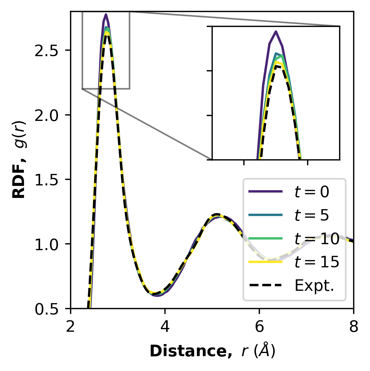
Figure 1: A pair potential correction added to the ANI MLP improves agreement with experimental RDF data for liquid aluminum at 1023 K. The experimental RDF is obtained from Ref. Kruglov et al., 2017. The RDF at generation $t=0$ (the original ANI model) is overstructured compared to the experiment. We use the wIBI update rule (1) with weights $w(r)=g_{E}(r)$, which biases corrections toward the peaks of the experimental RDFs.

The corrective potential is built iteratively. At each iteration $t$, an updated pair potential is calculated using the IBI update rule,

$$u^{t+1}(r) =u^{t}(r)+\alpha k_{B}T\ w(r)\ln\left[\frac{g^{t}(r)}{g_{E}(r)}\right],$$ (1)

which we have modified to include an arbitrary weight function $w(r)$. We select a relatively small learning rate $\alpha=2\times 10^{-4}$ which aids in the smoothness of the corrective potential. $g_{E}(r)$ is the experimental RDF. $g^{t}(r)$ is the simulated RDF, generated using the sum of the MLP and corrective potential $u^{t}(r)$. At the zeroth generation there is not yet a correction, $u^{t=0}=0$, such that $g^{t=0}$ corresponds to the simulated RDF for the original MLP. For our numerical implementation of $u(r)$, we use Akima splines Akima (1970). The Akima interpolation method uses a continuously differentiable sub-spline built from piece-wise cubic polynomials so that both $u(r)$ and its first derivative are continuous. For every iteration step $t$ when corrective potential is updated, then the MD is performed in the NPT ensemble to allow the system to equilibrate to the new density. Then RDFs for the next iteration are averaged over 100 configurations over a $10$ ps trajectory to ensure smoothness.

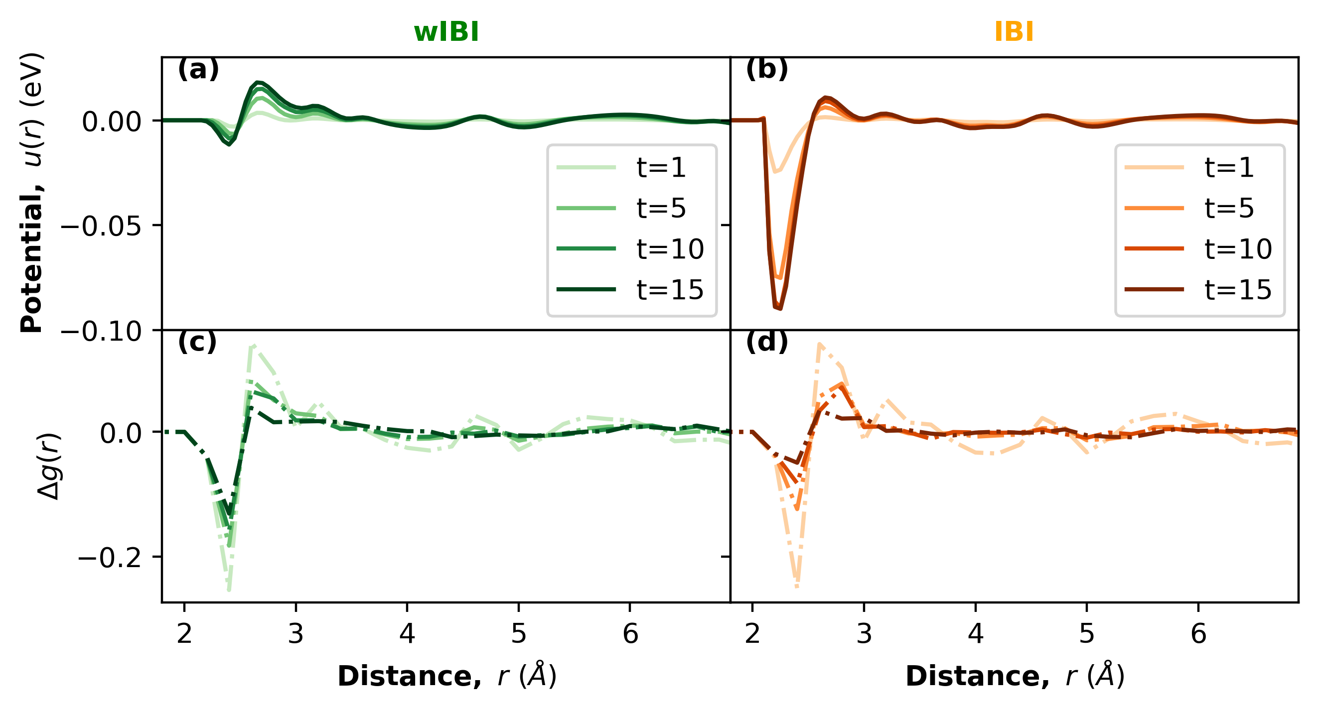
Figure 2: The wIBI approach avoids large, unphysical corrections to the pair potential at small distances. The general update rule for the corrective pair potential is defined in Eq. (1). The wIBI method of the left column uses $w(r)=g_{E}(r)$, whereas the traditional IBI method of the right column uses $w(r)=1$. Top row: the corrective pair potential $u^{t}(r)$ as a function of training iteration $t$. Bottom row: the resulting deviations $\Delta g(r)$ between the simulated and experimental RDF data. The wIBI and IBI corrections are mostly similar, but wIBI avoids large, unphysical corrections at distances $r$ below $2.5$$\mathrm{\text{Å}}$.

In the original IBI method, the weight function is $w(r)=1$. In our variant of this method, which we call the weighted Iterative Boltzmann Inversion (wIBI), we select $w(r)=g_{E}(r)$. In the limit $t\to\infty$, both IBI and wIBI should converge to the same corrective potential $u(r)$ that yields a perfect simulated RDF Jadrich et al. (2017). At early iterations $t$, however, there can be significant differences. By design, the wIBI method effectively ignores errors in the RDF at very small $r$, which may be associated with experimental uncertainty Soper (2013), and favors corrections at the RDF peaks. We further truncate $u(r)$ beyond $10$ $\mathrm{\text{Å}}$ because $g_{E}(r)\to 1$ for all temperatures considered. Other functional forms for the weight $w(r)$ may be used, provided that $w(r)$ is positive semi-definite and $w(r)>0$ for all $r$ where the experimental RDF is non-zero.

Figure 1 shows how the corrective potential $u^{t}(r)$ generated using the wIBI method results in improved match with the experimental RDF at $1023$ K Kruglov et al. (2017). The overstructured ANI-MLP simulated RDF (zeroth generation) is evident in the inset of Fig. 1. By the $15$th generation, the first shell peak matches the experimental results. Figure 2 compares the wIBI ($w(r)=g_{E}(r)$) and IBI ($w(r)=1$). For $r>3$ $\mathrm{\text{Å}}$, $u(r)$ for both wIBI and IBI is similar. The shape of $u(r)$ reflects the initial differences between the original MLP RDF and the experimental one, $\Delta g(r)=g_{r}^{t=0}(r)-g_{E}(r)$.

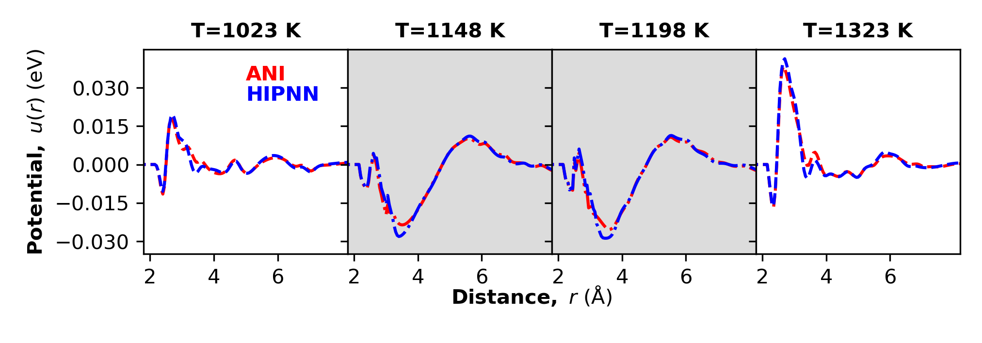
Figure 3: Similar corrective potentials are learned for two distinct neural network architectures, HIP-NN and ANI. The shape of $u^{t=15}(r)$ is determined by the MLP simulated RDFs, which are overstructured in either first or second shell, compared to $g_{E}(r)$. The white and gray backgrounds indicate corrective potentials trained to experimental RDF data from Refs. Kruglov et al., 2017 and Jakse and Pasturel, 2013, respectively.

Compared to the experimental RDFs, the ANI and HIP-NN simulated RDFs are overstructured for all temperatures between $943\mathrm{K}$ up to $1323\mathrm{K}$ obtained from different experiments Kruglov et al. (2017); Mauro et al. (2011). The RDFs for $1023\ \mathrm{K}$ and $1323\ \mathrm{K}$ show overstructuring in the first shell, whereas for $1148\ \mathrm{K}$ and $198\ \mathrm{K}$, the second shell is overstructured as well. In Fig. 3, the corrective potentials $u^{t=15}(r)$ at the $15$th generation of wIBI for both ANI and HIP-NN for $1023\ \mathrm{K}$, $1148\ \mathrm{K}$, $1198\ \mathrm{K}$, and $1323\ \mathrm{K}$ highlight that larger corrections are needed at higher temperatures. In Fig. 3, the shape of $u(r)$ reflects the corresponding $\Delta g(r)$, namely, the differences between the MLP RDF and the experimental one. Given that the correction required is very similar for ANI and HIP-NN, we attribute the MLP simulated overstructured RDF to limitations of the DFT method used for the training data. Similar overstructured RDFs for DFT and other ab initio methods have been observed in metals Jakse and Pasturel (2013) and water Gillan et al. (2016); Chen et al. (2017); Li et al. (2022). Typically, DFT functionals are well parameterized for near-equilibrium configurations and may perform poorly for the high temperature liquid phase. While improved DFT functionals can potentially alleviate some of these issues, our work presents a data driven correction, which may be readily applied to other systems Chen et al. (2017); Li et al. (2022).

4 Out of Sample Validation

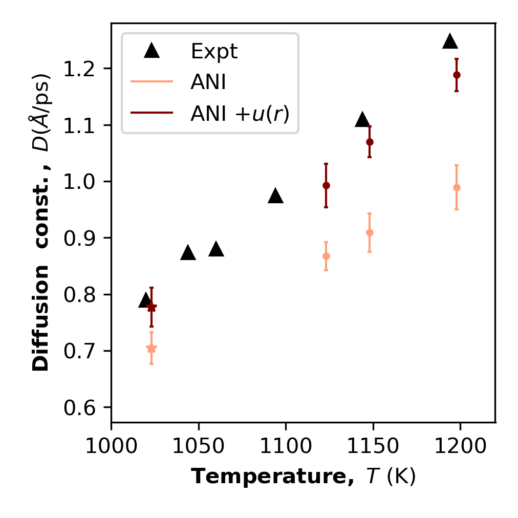
Figure 4: The corrective potential $u(r)$ improves predictions for the diffusion constant $D$. The $u(r)$ is trained only to RDF data, whereas $D$ is a dynamical property of the liquid phase. The diffusion constants are reported in Refs. Kargl et al. (2012); Jakse and Pasturel (2013). The corrected ML potentials are the same as in Fig. 3.

To validate our results, we compare the diffusion constants calculated for both the ANI and HIP-NN MLPs with and without the IBI corrective potential $u(r)$ at different temperatures. We measure the diffusion constants by averaging over 30 trajectories of length $1$ ps, and $1000$ snapshots. We fit the simulated trajectory to the Einstein Equation to infer the diffusion constant using Atomic Simulation Environment codebase Larsen et al. (2017).

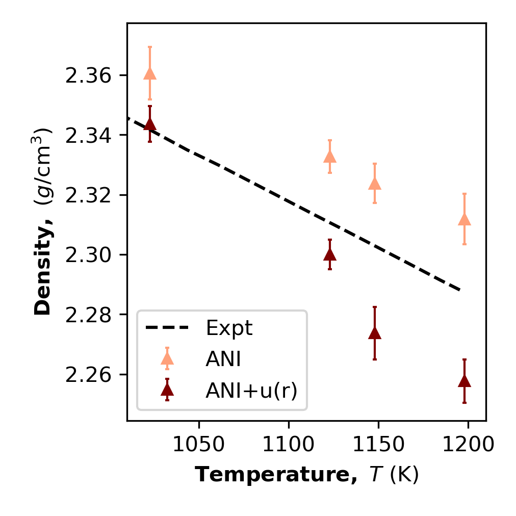
Figure 5: The corrective potential $u(r)$ improves predictions for the density of liquid aluminum. The corrected ML potentials are the same as in Fig. 3. The experimental densities is the line of best-fit as reported in Ref. Smith et al. (1999)

Figure 4 shows that the ANI MLP diffusion constants are underestimated compared to the data from two different experiments Jakse and Pasturel (2013); Kargl et al. (2012) for all temperatures. The ANI and HIP-NN (not shown) MLPs underestimate relation between the diffusion and temperature; the slope relating the diffusion constant $D$ to temperature $T$ differs from the experiment by approximately a factor of two. The underestimated diffusion constant is physically consistent with MLPs’ overstructured RDFs prediction. As expected the deviation between the DFT-based MLP prediction and experimental diffusion constant decreases with temperature. For each temperature, $u(r)$ improves the MLP simulated over-structured RDF and underestimated diffusion constant. We find that that $u(r)$ improves the predictions of both MLPs. The ANI MLP overestimate of equilibrium densities in the melt phase, as seen in Fig. 5, are partially corrected by the Note that the $u(r)$ is trained only to the RDF, which is an equilibrium statistic, independent of dynamics. In contrast, the diffusion constant is a dynamical property. Noticeable improvements in the predictions of an ‘out-of-sample’ dynamical observable is strong evidence that the IBI corrective potential is physically meaningful.

We find that extrapolating the corrective pair potential to temperatures beyond the experimental training data can lead to incorrect predictions. The high temperature corrective potentials we trained at $u(r;T=1023)$ and $u(r;T=1323)$ are ineffective when extrapolated to the solid phase. Either of these corrections worsens MLP predictions of zero-temperature properties such as lattice constants, and cold curves. Near the aluminum melting point of 933 K, the corrective potentials have a more neutral effect. The original ANI MLP predicts a melting temperature of $920\pm 5\mathrm{K}$, and adding the $u(r;T=1023)$ corrective potential does not alter this. However, adding the $u(r;T=1323)$ correction lowers the melting temperature to $905\pm 5\mathrm{K}$, which is further from the true experimental value. The corrections derived for the higher-temperature melt phase are not found to be helpful at lower temperatures. As such, care should be taken when applying the IBI rectifications, which are only applicable to the MLP simulations for a relevant temperature regime.

5 Conclusions

This study reports a method for generating a corrective pair potential for two distinct MLPs to match target experimental RDFs using the modified IBI technique. Compared to the traditional IBI method with a uniform $w(r)=1$ weight, our wIBI uses a distance dependent weight $w(r)=g_{\mathrm{E}}(r)$, which avoids unphysical corrections at small distances. Trained on to a DFT dataset alone Smith et al. (2021), both ANI and HIP-NN accurately reproduce DFT energies and forces, as well as cold-curves and lattice constants in the low-temperature solid crystalline phases. Adding a temperature dependent, corrective pair potential fixes the overstructured RDFs in the high temperature liquid phase. The improved predictions for diffusion constants indicate that the corrective potential is physically valid. These out of sample validation tests, such as diffusion constant predictions in this case, are important for any framework to incorporate experimental results into MLPs.

Our work does not require auto-differentiation through a MD solver and can be applied any MLP. Furthermore, the results are interpretable because the form of the pair potential relates to the differences in between the RDFs from simulation and experiment. If more experimental data is collected, it can be readily incorporated to further improve our results. Here, the wIBI potential $u(r)$ makes small corrections on top of an existing MLP. Future work could explore the efficacy of the method when there are significant deviations between the MLP and experimental RDFs. Another important consideration is that each wIBI corrective potential has been derived from experimental data for a specific temperature. Naive application of such a corrected MLP to new temperature regimes may yield poor accuracy. This is particularly evident when applying high temperature corrections to simulations at low temperature, as was shown in the aluminum examples.

In the future, we will extend our methods by using other inverse methods such as relative entropy minimization Jadrich et al. (2017); Thaler et al. (2022), or re-weighting techniques Bennett (1976); Shirts and Chodera (2008); Thaler and Zavadlav (2021). By combining the differentiable trajectory re-weighting technique Thaler and Zavadlav (2021) with our current methods, we may be able avoid long MD simulations when learning from experimental targets. Additionally, training to the three-body angular distribution function would be relevant for MLPs of water Li et al. (2022); Liu et al. (2022). We intend to explore how multi-state IBI methods Moore et al. (2014) may be used to fit to RDFs from different temperatures simultaneously and ideally provide continuous corrections to QM based MLPs.

Ultimately, this work is an example of how the experimental data can complement MLPs trained on ab initio data. By incorporating temperature-dependent corrective pair potentials, the resulting models allow for accurate simulations of aluminum in the melt phase. The magnitude of the learned corrections decreases monotonically with decreasing temperature. We did not, however, find any benefit in extrapolating these corrections to the solid phase, where the original MLP is known to be accurate Smith et al. (2021).

Acknowledgments

We acknowledge support from the US DOE, Office of Science, Basic Energy Sciences, Chemical Sciences, Geosciences, and Biosciences Division under Triad National Security, LLC (“Triad”) contract Grant 89233218CNA000001 (FWP: LANLE3F2). The research is performed in part at the Center for Nonlinear Studies (CNLS) and the Center for Integrated Nanotechnologies Nanotechnologies (CINT), a U.S. Department of Energy, Office of Science user facility at Los Alamos National Laboratory (LANL). This research used resources provided by the LANL Institutional Computing (IC) Program and the CCS-7 Darwin cluster at LANL. LANL is operated by Triad National Security, LLC, for the National Nuclear Security Administration of the U.S. Department of Energy (Contract No. 89233218NCA000001).

Appendix A Hyper-parameters

The ANI MLPs are implemented in the NeuroChem C++/CUDA software packages. Pre-compiled binaries for the ensemble of ANI-MLP is available for download ato . The he loss function is

$$\mathcal{L} =w_{\mathrm{energy}}(\hat{E}-E)^{2}+w_{\mathrm{force}}^{2}\sum_{j=1}^{3N}(\hat{\bm{f}}_{j}-\bm{f}_{j})^{2},$$ (2)

where $N$ is the number of atoms in a configuration or sample. Weight of $1.0$ and $0.01$ is used for the energy term and force terms respectively. Batch-size of $128$ was used. The ADAM update is used during training. The learning rate was initialized at $0.001$ and ultimately converged to $0.00001$, following the annealing schedule in Ref. Smith et al., 2017

All ANI-Al model symmetry function parameters are provided below:

⬇

Radial Cutoff (Radial): 7.0

Radial Cutoff (Angular): 5.0

Radial Eta: [43.9]

Radial Shift: [1.2500000, 1.4296875, 1.6093750, 1.7890625, 1.9687500, 2.1484375, 2.3281250, 2.5078125, 2.6875000, 2.8671875, 3.0468750, 3.2265625, 3.4062500, 3.5859375, 3.7656250, 3.9453125, 4.1250000, 4.3046875, 4.4843750, 4.6640625, 4.8437500, 5.0234375, 5.2031250, 5.3828125, 5.5625000, 5.7421875, 5.9218750, 6.1015625, 6.2812500, 6.4609375, 6.6406250, 6.8203125]

Angular Zeta: [69.4]

Angular Shift: [0.19634954, 0.58904862, 0.98174770, 1.3744468, 1.7671459, 2.1598449, 2.5525440, 2.9452431]

Angular Eta: [6.5]

Angular Radial Shift: [1.2500000, 1.7187500, 2.1875000, 2.6562500, 3.1250000, 3.5937500, 4.0625000, 4.5312500]

The HIP-NN Lubbers et al. (2018) MLP is implemented in PyTorch software package and is available for download lan . The loss function is

$$\mathcal{L} =100\times\mathrm{RMSE}_{\mathrm{energy-per-atom}}$$ (3)

$$+100\times\mathrm{MAE}_{\mathrm{energy-per-atom}}$$ (4)

$$+\mathrm{RMSE}_{\mathrm{forces}}$$ (5)

$$+\mathrm{MAE}_{\mathrm{forces}}+10^{-6}\times\sum_{i}w_{i}^{2},$$ (6)

where the last term corresponds to the $L2$ regularization with respect to the weights of the network. We use a network with $1$ interaction layer, $3$ atom layers (feed-forward layer) with a width of $15$ features. For the sensitivity functions, $20$ radial basis functions are used with a soft-min cutoff of $1.25~{}$\mathrm{\text{Å}}$$, the soft maximum cutoff of $7.0~{}$\mathrm{\text{Å}}$$, and hard maximum cutoff of $5~{}$\mathrm{\text{Å}}$$. We used the Adam Optimizer, with an initial learning rate of $0.001$, which is halved with a patience of $25$ epochs.

References

- Wang et al. (2014) Lee-Ping Wang, Alexey Titov, Robert McGibbon, Fang Liu, Vijay S Pande, and Todd J Martínez, “Discovering chemistry with an ab initio nanoreactor,” Nature Chemistry 6, 1044–1048 (2014).
- De Vivo et al. (2016) Marco De Vivo, Matteo Masetti, Giovanni Bottegoni, and Andrea Cavalli, “Role of molecular dynamics and related methods in drug discovery,” Journal of Medicinal Chemistry 59, 4035–4061 (2016).
- Steinhauser and Hiermaier (2009) Martin O Steinhauser and Stefan Hiermaier, “A review of computational methods in materials science: examples from shock-wave and polymer physics,” International journal of molecular sciences 10, 5135–5216 (2009).
- Sun et al. (2021) Liang Sun, Yu-Xing Zhou, Xu-Dong Wang, Yu-Han Chen, Volker L Deringer, Riccardo Mazzarello, and Wei Zhang, “Ab initio molecular dynamics and materials design for embedded phase-change memory,” npj Computational Materials 7, 1–8 (2021).
- Szabo and Ostlund (2012) Attila Szabo and Neil S Ostlund, Modern quantum chemistry: introduction to advanced electronic structure theory (Courier Corporation, 2012).
- Burke (2012) Kieron Burke, “Perspective on density functional theory,” The Journal of Chemical Physics 136, 150901 (2012).
- Behler and Parrinello (2007) Jörg Behler and Michele Parrinello, “Generalized neural-network representation of high-dimensional potential-energy surfaces,” Physical Review Letters 98, 146401 (2007).
- Bartók et al. (2010) Albert P Bartók, Mike C Payne, Risi Kondor, and Gábor Csányi, “Gaussian approximation potentials: The accuracy of quantum mechanics, without the electrons,” Physical Review Letters 104, 136403 (2010).
- Smith et al. (2017) Justin S Smith, Olexandr Isayev, and Adrian E Roitberg, “ANI-1: an extensible neural network potential with DFT accuracy at force field computational cost,” Chemical science 8, 3192–3203 (2017).
- Smith et al. (2018) Justin S Smith, Ben Nebgen, Nicholas Lubbers, Olexandr Isayev, and Adrian E Roitberg, “Less is more: Sampling chemical space with active learning,” The Journal of Chemical Physics 148, 241733 (2018).
- Lubbers et al. (2018) Nicholas Lubbers, Justin S Smith, and Kipton Barros, “Hierarchical modeling of molecular energies using a deep neural network,” The Journal of Chemical Physics 148, 241715 (2018).
- Unke and Meuwly (2019) Oliver T Unke and Markus Meuwly, “Physnet: A neural network for predicting energies, forces, dipole moments, and partial charges,” Journal of Chemical Theory and Computation 15, 3678–3693 (2019).
- Smith et al. (2019) Justin S Smith, Benjamin T Nebgen, Roman Zubatyuk, Nicholas Lubbers, Christian Devereux, Kipton Barros, Sergei Tretiak, Olexandr Isayev, and Adrian E Roitberg, “Approaching coupled cluster accuracy with a general-purpose neural network potential through transfer learning,” Nature Communications 10, 1–8 (2019).
- Zhang et al. (2019) Linfeng Zhang, De-Ye Lin, Han Wang, Roberto Car, and E Weinan, “Active learning of uniformly accurate interatomic potentials for materials simulation,” Physical Review Materials 3, 023804 (2019).
- Smith et al. (2021) Justin S Smith, Benjamin Nebgen, Nithin Mathew, Jie Chen, Nicholas Lubbers, Leonid Burakovsky, Sergei Tretiak, Hai Ah Nam, Timothy Germann, Saryu Fensin, et al., “Automated discovery of a robust interatomic potential for aluminum,” Nature Communications 12, 1–13 (2021).
- Unke et al. (2021a) Oliver T Unke, Stefan Chmiela, Michael Gastegger, Kristof T Schütt, Huziel E Sauceda, and Klaus-Robert Müller, “Spookynet: Learning force fields with electronic degrees of freedom and nonlocal effects,” Nature Communications 12, 1–14 (2021a).
- Deringer et al. (2021) Volker L Deringer, Albert P Bartók, Noam Bernstein, David M Wilkins, Michele Ceriotti, and Gábor Csányi, “Gaussian process regression for materials and molecules,” Chemical Reviews 121, 10073–10141 (2021).
- Zhang et al. (2022) Linfeng Zhang, Han Wang, Maria Carolina Muniz, Athanassios Z Panagiotopoulos, Roberto Car, and Weinan E, “A deep potential model with long-range electrostatic interactions,” The Journal of Chemical Physics 156, 124107 (2022).
- Fedik et al. (2022) Nikita Fedik, Roman Zubatyuk, Maksim Kulichenko, Nicholas Lubbers, Justin S Smith, Benjamin Nebgen, Richard Messerly, Ying Wai Li, Alexander I Boldyrev, Kipton Barros, , Olexandr Isayev, and Sergei Tretiak, “Extending machine learning beyond interatomic potentials for predicting molecular properties,” Nature Reviews Chemistry 6, 653–672 (2022).
- Kulichenko et al. (2021) Maksim Kulichenko, Justin S Smith, Benjamin Nebgen, Ying Wai Li, Nikita Fedik, Alexander I Boldyrev, Nicholas Lubbers, Kipton Barros, and Sergei Tretiak, “The rise of neural networks for materials and chemical dynamics,” The Journal of Physical Chemistry Letters 12, 6227–6243 (2021).
- Beckmann et al. (2022) Richard Beckmann, Fabien Brieuc, Christoph Schran, and Dominik Marx, “Infrared spectra at coupled cluster accuracy from neural network representations,” Journal of Chemical Theory and Computation 18, 5492–5501 (2022), pMID: 35998360, https://doi.org/10.1021/acs.jctc.2c00511 .
- Daru et al. (2022) János Daru, Harald Forbert, Jörg Behler, and Dominik Marx, “Coupled cluster molecular dynamics of condensed phase systems enabled by machine learning potentials: Liquid water benchmark,” Physical Review Letters 129, 226001 (2022).
- Batzner et al. (2022) Simon Batzner, Albert Musaelian, Lixin Sun, Mario Geiger, Jonathan P Mailoa, Mordechai Kornbluth, Nicola Molinari, Tess E Smidt, and Boris Kozinsky, “E(3)-equivariant graph neural networks for data-efficient and accurate interatomic potentials,” Nature Communications 13, 1–11 (2022).
- Podryabinkin and Shapeev (2017) Evgeny V Podryabinkin and Alexander V Shapeev, “Active learning of linearly parametrized interatomic potentials,” Computational Materials Science 140, 171–180 (2017).
- Deringer et al. (2018) Volker L Deringer, Chris J Pickard, and Gábor Csányi, “Data-driven learning of total and local energies in elemental boron,” Physical Review Letters 120, 156001 (2018).
- Jinnouchi et al. (2020) Ryosuke Jinnouchi, Kazutoshi Miwa, Ferenc Karsai, Georg Kresse, and Ryoji Asahi, “On-the-fly active learning of interatomic potentials for large-scale atomistic simulations,” The Journal of Physical Chemistry Letters 11, 6946–6955 (2020).
- Bernstein et al. (2019) Noam Bernstein, Gábor Csányi, and Volker L Deringer, “De novo exploration and self-guided learning of potential-energy surfaces,” npj Computational Materials 5, 1–9 (2019).
- Sivaraman et al. (2020) Ganesh Sivaraman, Anand Narayanan Krishnamoorthy, Matthias Baur, Christian Holm, Marius Stan, Gábor Csányi, Chris Benmore, and Álvaro Vázquez-Mayagoitia, “Machine-learned interatomic potentials by active learning: amorphous and liquid hafnium dioxide,” npj Computational Materials 6, 1–8 (2020).
- Montes de Oca Zapiain et al. (2022) David Montes de Oca Zapiain, Mitchell A Wood, Nicholas Lubbers, Carlos Z Pereyra, Aidan P Thompson, and Danny Perez, “Training data selection for accuracy and transferability of interatomic potentials,” npj Computational Materials 8, 1–9 (2022).
- Devereux et al. (2020) Christian Devereux, Justin S Smith, Kate K Huddleston, Kipton Barros, Roman Zubatyuk, Olexandr Isayev, and Adrian E Roitberg, “Extending the applicability of the ani deep learning molecular potential to sulfur and halogens,” Journal of Chemical Theory and Computation 16, 4192–4202 (2020).
- Fu et al. (2022) Xiang Fu, Zhenghao Wu, Wujie Wang, Tian Xie, Sinan Keten, Rafael Gomez-Bombarelli, and Tommi Jaakkola, “Forces are not enough: Benchmark and critical evaluation for machine learning force fields with molecular simulations,” arXiv preprint arXiv:2210.07237 (2022).
- van der Oord et al. (2022) Cas van der Oord, Matthias Sachs, Dávid Péter Kovács, Christoph Ortner, and Gábor Csányi, “Hyperactive learning (hal) for data-driven interatomic potentials,” arXiv preprint arXiv:2210.04225 (2022).
- Rupp et al. (2012) Matthias Rupp, Alexandre Tkatchenko, Klaus-Robert Müller, and O Anatole Von Lilienfeld, “Fast and accurate modeling of molecular atomization energies with machine learning,” Physical Review Letters 108, 058301 (2012).
- Craven et al. (2020) Galen T Craven, Nicholas Lubbers, Kipton Barros, and Sergei Tretiak, “Machine learning approaches for structural and thermodynamic properties of a lennard-jones fluid,” The Journal of Chemical Physics 153, 104502 (2020).
- Kovács et al. (2021) Dávid Péter Kovács, Cas van der Oord, Jiri Kucera, Alice EA Allen, Daniel J Cole, Christoph Ortner, and Gábor Csányi, “Linear atomic cluster expansion force fields for organic molecules: beyond RMSE,” Journal of chemical theory and computation 17, 7696–7711 (2021).
- Allen and Tkatchenko (2022) Alice EA Allen and Alexandre Tkatchenko, “Machine learning of material properties: Predictive and interpretable multilinear models,” Science Advances 8, eabm7185 (2022).
- Sifain et al. (2018) Andrew E Sifain, Nicholas Lubbers, Benjamin T Nebgen, Justin S Smith, Andrey Y Lokhov, Olexandr Isayev, Adrian E Roitberg, Kipton Barros, and Sergei Tretiak, “Discovering a transferable charge assignment model using machine learning,” The journal of physical chemistry letters 9, 4495–4501 (2018).
- Ko et al. (2021a) Tsz Wai Ko, Jonas A Finkler, Stefan Goedecker, and Jörg Behler, “A fourth-generation high-dimensional neural network potential with accurate electrostatics including non-local charge transfer,” Nature Communications 12, 1–11 (2021a).
- Jacobson et al. (2022) Leif D Jacobson, James M Stevenson, Farhad Ramezanghorbani, Delaram Ghoreishi, Karl Leswing, Edward D Harder, and Robert Abel, “Transferable neural network potential energy surfaces for closed-shell organic molecules: Extension to ions,” Journal of Chemical Theory and Computation 18, 2354–2366 (2022).
- Gao and Remsing (2022) Ang Gao and Richard C Remsing, “Self-consistent determination of long-range electrostatics in neural network potentials,” Nature Communications 13, 1–11 (2022).
- Eckhoff et al. (2020) Marco Eckhoff, Knut Nikolas Lausch, Peter E Blöchl, and Jörg Behler, “Predicting oxidation and spin states by high-dimensional neural networks: Applications to lithium manganese oxide spinels,” The Journal of Chemical Physics 153, 164107 (2020).
- Tu et al. (2023) Nguyen Thien Phuc Tu, Nazanin Rezajooei, Erin R. Johnson, and Christopher N. Rowley, “A neural network potential with rigorous treatment of long-range dispersion,” Digital Discovery 2, 718–727 (2023).
- Magedov et al. (2021) Sergey Magedov, Christopher Koh, Walter Malone, Nicholas Lubbers, and Benjamin Nebgen, “Bond order predictions using deep neural networks,” Journal of Applied Physics 129, 064701 (2021).
- Yao et al. (2018) Kun Yao, John E Herr, David W Toth, Ryker Mckintyre, and John Parkhill, “The tensormol-0.1 model chemistry: a neural network augmented with long-range physics,” Chemical science 9, 2261–2269 (2018).
- Behler and Csányi (2021) Jörg Behler and Gábor Csányi, “Machine learning potentials for extended systems: a perspective,” The European Physical Journal B 94, 1–11 (2021).
- Ko et al. (2021b) Tsz Wai Ko, Jonas A Finkler, Stefan Goedecker, and Jorg Behler, “General-purpose machine learning potentials capturing nonlocal charge transfer,” Accounts of Chemical Research 54, 808–817 (2021b).
- Unke et al. (2021b) Oliver T Unke, Stefan Chmiela, Huziel E Sauceda, Michael Gastegger, Igor Poltavsky, Kristof T Schütt, Alexandre Tkatchenko, and Klaus-Robert Müller, “Machine learning force fields,” Chemical Reviews 121, 10142–10186 (2021b).
- Kobayashi et al. (2017) Ryo Kobayashi, Daniele Giofré, Till Junge, Michele Ceriotti, and William A Curtin, “Neural network potential for al-mg-si alloys,” Physical Review Materials 1, 053604 (2017).
- Botu et al. (2017) Venkatesh Botu, Rohit Batra, James Chapman, and Rampi Ramprasad, “Machine learning force fields: construction, validation, and outlook,” The Journal of Physical Chemistry C 121, 511–522 (2017).
- Kruglov et al. (2017) Ivan Kruglov, Oleg Sergeev, Alexey Yanilkin, and Artem R Oganov, “Energy-free machine learning force field for aluminum,” Scientific reports 7, 1–7 (2017).
- Mauro et al. (2011) NA Mauro, JC Bendert, AJ Vogt, JM Gewin, and KF Kelton, “High energy x-ray scattering studies of the local order in liquid al,” The Journal of Chemical Physics 135, 044502 (2011).
- Mendelev et al. (2008) MI Mendelev, MJ Kramer, Chandler A Becker, and M Asta, “Analysis of semi-empirical interatomic potentials appropriate for simulation of crystalline and liquid al and cu,” Philosophical Magazine 88, 1723–1750 (2008).
- Jakse and Pasturel (2013) Noel Jakse and Alain Pasturel, “Liquid aluminum: Atomic diffusion and viscosity from ab initio molecular dynamics,” Scientific Reports 3, 1–8 (2013).
- Chen et al. (2017) Mohan Chen, Hsin-Yu Ko, Richard C Remsing, Marcos F Calegari Andrade, Biswajit Santra, Zhaoru Sun, Annabella Selloni, Roberto Car, Michael L Klein, John P Perdew, et al., “Ab initio theory and modeling of water,” Proceedings of the National Academy of Sciences 114, 10846–10851 (2017).
- Liu et al. (2020) Qianrui Liu, Denghui Lu, and Mohan Chen, “Structure and dynamics of warm dense aluminum: a molecular dynamics study with density functional theory and deep potential,” Journal of Physics: Condensed Matter 32, 144002 (2020).
- Li et al. (2022) Chenghan Li, Francesco Paesani, and Gregory A Voth, “Static and dynamic correlations in water: Comparison of classical ab initio molecular dynamics at elevated temperature with path integral simulations at ambient temperature,” Journal of Chemical Theory and Computation 18, 2124–2131 (2022).
- Gillan et al. (2016) Michael J Gillan, Dario Alfe, and Angelos Michaelides, “Perspective: How good is dft for water?” The Journal of Chemical Physics 144, 130901 (2016).
- Note (1) It seems possible that the nearsightedness assumption of traditional MLPs excludes information that would be important to make a determination about the electronic structure of the global many-body quantum state.
- Thaler and Zavadlav (2021) Stephan Thaler and Julija Zavadlav, “Learning neural network potentials from experimental data via differentiable trajectory reweighting,” Nature Communications 12, 1–10 (2021).
- Fröhlking et al. (2020) Thorben Fröhlking, Mattia Bernetti, Nicola Calonaci, and Giovanni Bussi, “Toward empirical force fields that match experimental observables,” The Journal of Chemical Physics 152, 230902 (2020).
- Ingraham et al. (2018) John Ingraham, Adam Riesselman, Chris Sander, and Debora Marks, “Learning protein structure with a differentiable simulator,” in International Conference on Learning Representations (2018).
- Doerr et al. (2021) Stefan Doerr, Maciej Majewski, Adrià Pérez, Andreas Kramer, Cecilia Clementi, Frank Noe, Toni Giorgino, and Gianni De Fabritiis, “Torchmd: A deep learning framework for molecular simulations,” Journal of chemical theory and computation 17, 2355–2363 (2021).
- Schoenholz and Cubuk (2021) Samuel S Schoenholz and Ekin D Cubuk, “Jax, md a framework for differentiable physics,” Journal of Statistical Mechanics: Theory and Experiment 2021, 124016 (2021).
- Wang et al. (2023) Wujie Wang, Zhenghao Wu, Johannes CB Dietschreit, and Rafael Gómez-Bombarelli, “Learning pair potentials using differentiable simulations,” The Journal of Chemical Physics 158 (2023), https://doi.org/10.1063/5.0126475.
- Müller-Plathe (2002) Florian Müller-Plathe, “Coarse-graining in polymer simulation: from the atomistic to the mesoscopic scale and back,” ChemPhysChem 3, 754–769 (2002).
- Noid (2013) William George Noid, “Perspective: Coarse-grained models for biomolecular systems,” The Journal of Chemical Physics 139, 090901 (2013).
- Lindquist et al. (2016) Beth A Lindquist, Ryan B Jadrich, and Thomas M Truskett, “Communication: Inverse design for self-assembly via on-the-fly optimization,” The Journal of Chemical Physics 145, 111101 (2016).
- Jadrich et al. (2017) R. B. Jadrich, B. A. Lindquist, and T. M. Truskett, “Probabilistic inverse design for self-assembling materials,” The Journal of Chemical Physics 146, 184103 (2017).
- Sherman et al. (2020) Zachary M Sherman, Michael P Howard, Beth A Lindquist, Ryan B Jadrich, and Thomas M Truskett, “Inverse methods for design of soft materials,” The Journal of Chemical Physics 152, 140902 (2020).
- Marcotte et al. (2011) Étienne Marcotte, Frank H Stillinger, and Sal Torquato, “Unusual ground states via monotonic convex pair potentials,” The Journal of Chemical Physics 134, 164105 (2011).
- Gubaev et al. (2018) Konstantin Gubaev, Evgeny V Podryabinkin, and Alexander V Shapeev, “Machine learning of molecular properties: Locality and active learning,” The Journal of Chemical Physics 148, 241727 (2018).
- (72) ANI-AL data and model, available online: https://github.com/atomistic-ml/ani-al.
- Davey (1925) Wheeler P Davey, “Precision measurements of the lattice constants of twelve common metals,” Physical Review 25, 753 (1925).
- (74) The Lava wrapper, available online: https://github.com/lanl/LAVA.
- Larsen et al. (2017) Ask Hjorth Larsen, Jens Jørgen Mortensen, Jakob Blomqvist, Ivano E Castelli, Rune Christensen, Marcin Dułak, Jesper Friis, Michael N Groves, Bjørk Hammer, Cory Hargus, et al., “The atomic simulation environment—a python library for working with atoms,” Journal of Physics: Condensed Matter 29, 273002 (2017).
- Akima (1970) Hiroshi Akima, “A new method of interpolation and smooth curve fitting based on local procedures,” Journal of the ACM (JACM) 17, 589–602 (1970).
- Soper (2013) Alan K Soper, “The radial distribution functions of water as derived from radiation total scattering experiments: Is there anything we can say for sure?” International Scholarly Research Notices 2013 (2013), https://doi.org/10.1155/2013/279463.
- Kargl et al. (2012) F Kargl, H Weis, T Unruh, and A Meyer, “Self diffusion in liquid aluminium,” in Journal of Physics: Conference Series, Vol. 340 (IOP Publishing, 2012) p. 012077.
- Smith et al. (1999) Patrick M Smith, John W Elmer, and Gilbert F Gallegos, “Measurement of the density of liquid aluminum alloys by an x-ray attenuation technique,” Scripta materialia 40, 937–941 (1999).
- Thaler et al. (2022) Stephan Thaler, Maximilian Stupp, and Julija Zavadlav, “Deep coarse-grained potentials via relative entropy minimization,” The Journal of Chemical Physics (2022), https://doi.org/10.1063/5.0124538.
- Bennett (1976) Charles H Bennett, “Efficient estimation of free energy differences from monte carlo data,” Journal of Computational Physics 22, 245–268 (1976).
- Shirts and Chodera (2008) Michael R Shirts and John D Chodera, “Statistically optimal analysis of samples from multiple equilibrium states,” The Journal of Chemical Physics 129, 124105 (2008).
- Liu et al. (2022) Jinfeng Liu, Jinggang Lan, and Xiao He, “Toward high-level machine learning potential for water based on quantum fragmentation and neural networks,” The Journal of Physical Chemistry A (2022), https://doi.org/10.1021/acs.jpca.2c00601.
- Moore et al. (2014) Timothy C Moore, Christopher R Iacovella, and Clare McCabe, “Derivation of coarse-grained potentials via multistate iterative boltzmann inversion,” The Journal of Chemical Physics 140, 06B606_1 (2014).
- (85) The hippynn package - a modular library for atomistic machine learning with PyTorch, available online: https://github.com/lanl/hippynn.