Topological recursion of the Weil–Petersson volumes of hyperbolic surfaces with tight boundaries

Abstract

The Weil–Petersson volumes of moduli spaces of hyperbolic surfaces with geodesic boundaries are known to be given by polynomials in the boundary lengths. These polynomials satisfy Mirzakhani’s recursion formula, which fits into the general framework of topological recursion. We generalize the recursion to hyperbolic surfaces with any number of special geodesic boundaries that are required to be tight. A special boundary is tight if it has minimal length among all curves that separate it from the other special boundaries. The Weil–Petersson volume of this restricted family of hyperbolic surfaces is shown again to be polynomial in the boundary lengths. This remains true when we allow conical defects in the surface with cone angles in $(0,\pi)$ in addition to geodesic boundaries. Moreover, the generating function of Weil–Petersson volumes with fixed genus and a fixed number of special boundaries is polynomial as well, and satisfies a topological recursion that generalizes Mirzakhani’s formula.

This work is largely inspired by recent works by Bouttier, Guitter & Miermont on the enumeration of planar maps with tight boundaries. Our proof relies on the equivalence of Mirzakhani’s recursion formula to a sequence of partial differential equations (known as the Virasoro constraints) on the generating function of intersection numbers.

Finally, we discuss a connection with JT gravity. We show that the multi-boundary correlators of JT gravity with defects (cone points or FZZT branes) are expressible in the tight Weil–Petersson volume generating functions, using a tight generalization of the JT trumpet partition function.

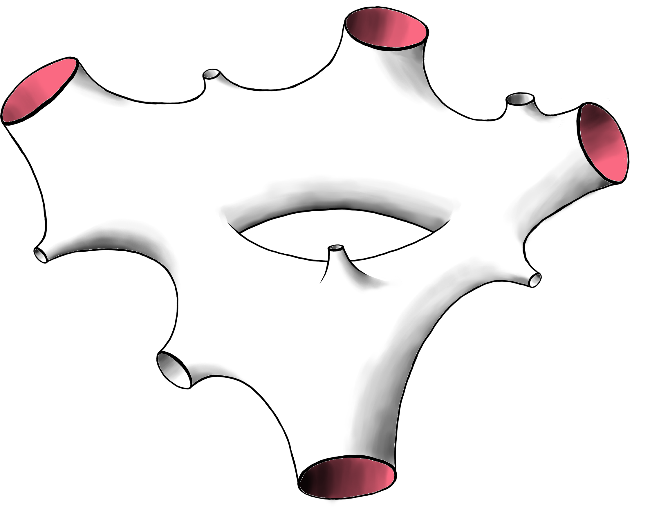
Figure 1: An example of a genus-$1$ hyperbolic surface with four tight boundaries (in pink).

1 Introduction

1.1 Topological recursion of Weil–Petersson volumes

In the celebrated work [Mirzakhani2007] Mirzakhani established a recursion formula for the Weil–Petersson volume $V_{g,n}(\mathbf{L})$ of the moduli space of genus-$g$ hyperbolic surfaces with $n$ labeled boundaries of lengths $\mathbf{L}=(L_{1},\ldots,L_{n})\in\mathbb{R}_{>0}^{n}$. Denoting $[n]=\{1,2,\ldots,n\}$ and using the notation $\mathbf{L}_{I}=(L_{i})_{i\in I}$, $I\subset[n]$, for a subsequence of $\mathbf{L}$ and $\mathbf{L}_{\widehat{I}}=\mathbf{L}_{[n]\setminus I}$, the recursion can be expressed for $(g,n)\notin\{(0,3),(1,1)\}$ as

$$V_{g,n}(\mathbf{L}) =\frac{1}{2L_{1}}\int_{0}^{L_{1}}\differential{t}\int_{0}^{\infty}\differential{x}\int_{0}^{\infty}\differential{y}\,xyK_{0}(x+y,t)\Bigg{[}V_{g-1,n+1}(x,y,\mathbf{L}_{\widehat{\{1\}}})$$

$$\mkern 370.0mu+\!\!\!\!\sum_{\begin{subarray}{c}g_{1}+g_{2}=g\\ I\amalg J=\{2,\ldots,n\}\end{subarray}}V_{g_{1},1+|I|}(x,\mathbf{L}_{I})V_{g_{2},1+|J|}(y,\mathbf{L}_{J})\Bigg{]}$$

$$+\frac{1}{2L_{1}}\int_{0}^{L_{1}}\differential{t}\int_{0}^{\infty}\differential{x}\sum_{j=2}^{n}\,x\left(K_{0}(x,t+L_{j})+K_{0}(x,t-L_{j})\right)V_{g,n-1}(x,\mathbf{L}_{\widehat{\{1,j\}}}),$$ (1)

where

$$K_{0}(x,t) =\frac{1}{1+\exp(\frac{x+t}{2})}+\frac{1}{1+\exp(\frac{x-t}{2})}.$$ (2)

Together with $V_{0,3}(\mathbf{L})=1$ and $V_{1,1}(\mathbf{L})=\frac{L_{1}^{2}}{48}+\frac{\pi^{2}}{12}$ this completely determines $V_{g,n}$ as a symmetric polynomial in $L_{1}^{2},\ldots,L_{n}^{2}$ of degree $3g-3+n$.

This recursion formula remains valid [Tan_Generalizations_2006, Mirzakhani2007] when we replace one or more of the boundaries by cone points with cone angle $\alpha_{i}\in(0,\pi)$ if we assign to it an imaginary boundary length $L_{i}=i\alpha_{i}$. Cone points with angles in $(0,\pi)$ are called sharp, as opposed to blunt cone points that have angle in $(\pi,2\pi)$. The Weil–Petersson volume of the moduli space of genus-$g$ surfaces with $n$ geodesic boundaries or sharp cone points is thus correctly computed by the polynomial $V_{g,n}(\mathbf{L})$.

It was recognized by Eynard & Orantin [eynard2007weil] that Mirzakhani’s recursion (in the case of geodesic boundaries) fits the general framework of topological recursion. To state this result explicitly one introduces for any $g,n\geq 0$ satisfying $3g-3+n\geq 0$ the Laplace transformed Weil–Petersson volumes

$$\omega_{g,n}^{(0)}(\mathbf{z})=\int_{0}^{\infty}\left[\prod_{i=1}^{n}\mathrm{d}L_{i}\,L_{i}e^{-z_{i}L_{i}}\right]V_{g,n}(\mathbf{L}),$$ (3)

which are even polynomials in $z_{1}^{-1},\ldots,z_{n}^{-1}$ of degree $6g-4+2n$, while setting

$$\omega_{0,1}^{(0)}(\mathbf{z})=0,\qquad\omega_{0,2}^{(0)}(\mathbf{z})=\frac{1}{(z_{1}-z_{2})^{2}}.$$ (4)

Then Mirzakhani’s recursion (1) translates into the recursion [eynard2007weil, Theorem 2.1]

$$\omega_{g,n}^{(0)}(\mathbf{z})=\operatorname*{Res}_{u\to 0}\frac{\pi}{(z_{1}^{2}-u^{2})\sin 2\pi u}\Bigg{[}\omega^{(0)}_{g-1,n+1}(u,-u,\mathbf{z}_{\widehat{\{1\}}})+\sum_{\begin{subarray}{c}g_{1}+g_{2}=g\\ I\amalg J=\{2,\ldots,n\}\end{subarray}}\omega^{(0)}_{g_{1},1+|I|}(u,\mathbf{z}_{I})\omega^{(0)}_{g_{2},1+|J|}(-u,\mathbf{z}_{J})\Bigg{]}$$ (5)

valid when $g,n\geq 0$ and $3g-3+n\geq 0$, which one may recognize as the recursion for the invariants $\omega^{(0)}_{g,n}(\mathbf{z})$ of the complex curve

$$\begin{dcases}x(z)=z^{2}\\ y(z)=\frac{1}{\pi}\sin(2\pi z).\end{dcases}$$ (6)

The main purpose of the current work is to generalize these recursion formulas to hyperbolic surfaces with so-called tight boundaries, which we introduce now.

1.2 Hyperbolic surfaces with tight boundaries

Let $S_{g,n}$ be a fixed topological surface of genus $g$ with $n$ boundaries and $\mathcal{T}_{g,n}(\mathbf{L})$ the Teichmüller space of hyperbolic structures on $S_{g,n}$ with geodesic boundaries of lengths $\mathbf{L}=(L_{1},\ldots,L_{n})\in\mathbb{R}_{>0}^{n}$. Denote the boundary cycles by $\partial_{1},\ldots,\partial_{n}$ and the free homotopy class of a cycle $\gamma$ in $S_{g,n}$ by $[\gamma]_{S_{g,n}}$. For a hyperbolic surface $X\in\mathcal{T}_{g,n}(\mathbf{L})$ and a cycle $\gamma$, we denote by $\ell_{\gamma}(X)$ the length of $\gamma$, in particular $\ell_{\partial_{i}}(X)=L_{i}$. The mapping class group of $S_{g,n}$ is denoted $\mathrm{Mod}_{g,n}$ and the quotient of $\mathcal{T}_{g,n}(\mathbf{L})$ by its action leads to the moduli space

$$\mathcal{M}_{g,n}(\mathbf{L})=\mathcal{T}_{g,n}(\mathbf{L})/\mathrm{Mod}_{g,n}.$$

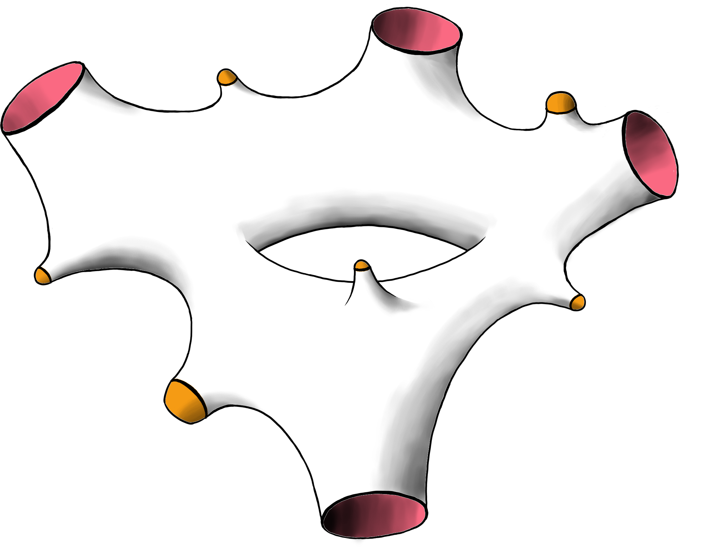
Figure 2: A surface $S_{g,n+p}$ (left) and the result $\invbreve{S}_{g,n,p}$ (right) of capping off the last $p$ boundaries, with in this case $g=1$, $n=4$ and $p=6$. If the original surface was equipped with a hyperbolic structure, it is natural to think of the resulting surface as the Riemannian manifold obtained by attaching constantly curved hemispheres of appropriate diameter to the $p$ geodesic boundaries.

Let us denote by $\invbreve{S}_{g,n,p}\supset S_{g,n+p}$ the topological surface obtained from $S_{g,n+p}$ by capping off the last $p$ boundaries with disks (Figure 2). Note that the free homotopy classes $[\cdot]_{S_{g,n+p}}$ of $S_{g,n+p}$ are naturally partitioned into the free homotopy classes $[\cdot]_{\invbreve{S}_{g,n,p}}$ of $\invbreve{S}_{g,n,p}$. In particular, $[\partial_{j}]_{S_{g,n+p}}$ for $j=n+1,\ldots,n+p$ are all contained in the null-homotopy class of $\invbreve{S}_{g,n,p}$. For $i=1,\ldots,n$ the boundary $\partial_{i}$ of $X\in\mathcal{M}_{g,n+p}(\mathbf{L})$ is said to be tight in $\invbreve{S}_{g,n,p}$ if $\partial_{i}$ is the only simple cycle $\gamma$ in $[\partial_{i}]_{\invbreve{S}_{g,n,p}}$ of length $\ell_{\gamma}(X)\leq L_{i}$. Remark that both $[\partial_{i}]_{S_{g,n+p}}$ and $[\partial_{i}]_{\invbreve{S}_{g,n,p}}$ for $i=1,\ldots,n$ are $\mathrm{Mod}_{g,n+p}$-invariant, so these classes are well-defined at the level of the moduli space. This allows us to introduce the moduli space of tight hyperbolic surfaces

$$\mathcal{M}^{\text{tight}}_{g,n,p}(\mathbf{L}) =\{X\in\mathcal{M}_{g,n+p}(\mathbf{L}):\partial_{1},\ldots,\partial_{n}\text{ are tight in }\invbreve{S}_{g,n,p}\}\subset\mathcal{M}_{g,n+p}(\mathbf{L}).$$ (7)

Note that $\mathcal{M}^{\text{tight}}_{g,n,0}(\mathbf{L})=\mathcal{M}^{\text{tight}}_{g,0,n}(\mathbf{L})=\mathcal{M}_{g,n}(\mathbf{L})$, while $\mathcal{M}^{\text{tight}}_{0,1,p}(\mathbf{L})=\emptyset$ because $\partial_{1}$ is null-homotopic and $\mathcal{M}^{\text{tight}}_{0,2,p}(\mathbf{L})=\emptyset$ because $[\partial_{1}]_{\invbreve{S}_{0,2,p}}=[\partial_{2}]_{\invbreve{S}_{0,2,p}}$ and therefore $\partial_{1}$ and $\partial_{2}$ can never both be the unique shortest cycle in their class. In general, it is an open subset of $\mathcal{M}_{g,n+p}(\mathbf{L})$ and therefore it inherits the Weil–Petersson symplectic structure and Weil–Petersson measure $\mathrm{d}\mu_{\mathrm{WP}}$ from $\mathcal{M}_{g,n+p}(\mathbf{L})$. The corresponding tight Weil–Petersson volumes are denoted

$$T_{g,n,p}(\mathbf{L})=\int_{\mathcal{M}^{\text{tight}}_{g,n,p}(\mathbf{L})}\mathrm{d}\mu_{\mathrm{WP}}\quad\leq\quad V_{g,n+p}(\mathbf{L}),$$ (8)

such that $T_{g,n,0}(\mathbf{L})=T_{g,0,n}(\mathbf{L})=V_{g,n}(\mathbf{L})$ and $T_{0,1,p}(\mathbf{L})=T_{0,2,p}(\mathbf{L})=0$.

We can extend this definition to the case in which one or more of the boundaries $\partial_{n+1},\ldots,\partial_{n+p}$ is replaced by a sharp cone point with cone angle $\alpha_{i}\in(0,\pi)$. In this case we make the usual identification $L_{i}=i\alpha_{i}$, and still denote the corresponding Weil–Petersson volume by $T_{g,n,p}(\mathbf{L})$. Our first result is the following.

Proposition 1.

For $g,n,p\geq 0$ such that $3g-3+n\geq 0$, the tight Weil–Petersson volume $T_{g,n,p}(\mathbf{L})$ of genus $g$ surfaces with $n$ tight boundaries and $p$ geodesic boundaries or sharp cone points is a polynomial in $L_{1}^{2},\ldots,L_{n+p}^{2}$ of degree $3g-3+n+p$ that is symmetric in $L_{1},\ldots,L_{n}$ and symmetric in $L_{n+1},\ldots,L_{n+p}$.

For most of the upcoming results we maintain the intuitive picture that the tight boundaries are the “real” boundaries of the surface, whose number and lengths we specify, while we allow for an arbitrary number of other boundaries or cone points that we treat as defects in the surface. To this end we would like to encode the volume polynomials in generating functions that sum over the number of defects with appropriate weights. A priori it is not entirely clear what is the best way to organize such generating functions, so to motivate our definition we take a detour to a natural application of Weil–Petersson volumes in random hyperbolic surfaces.

1.3 Intermezzo: Random (tight) hyperbolic surfaces

If we fix $g$, $n$ and $\mathbf{L}\in([0,\infty)\cup i(0,\pi))^{n}$, then upon normalization by $1/V_{g,n}(\mathbf{L})$ the Weil–Petersson measure $\mathrm{d}\mu_{\mathrm{WP}}$ provides a well-studied probability measure on $\mathcal{M}_{g,n}(\mathbf{L})$ defining the Weil–Petersson random hyperbolic surface, see e.g. [Mirzakhani_Growth_2013, Guth_Pants_2011, Mirzakhani_Lengths_2019, Gilmore_Short_2021, Monk_Benjamini_2022]. A natural way to extend the randomness to the boundary lengths or cone angles is by choosing a (Borel) measure $\mu$ on $[0,\infty)\cup i(0,\pi)$ and first sampling $\mathbf{L}\in([0,\infty)\cup i(0,\pi))^{n}$ from the probability measure

$$\frac{1}{\mu^{\otimes n}(V_{g,n})}V_{g,n}(\mathbf{L})\mathrm{d}\mu(L_{1})\cdots\mathrm{d}\mu(L_{n}),\quad\mu^{\otimes n}(V_{g,n})\coloneqq\int V_{g,n}(\mathbf{L})\mathrm{d}\mu(L_{1})\cdots\mathrm{d}\mu(L_{n}),$$ (9)

and then sampling a Weil–Petersson random hyperbolic surface on $\mathcal{M}_{g,n}(\mathbf{L})$. If the genus-$g$ partition function

$$F_{g}[\mu]=\sum_{n\geq 0}\frac{\mu^{\otimes n}(V_{g,n})}{n!}$$ (10)

converges, we can furthermore make the size $n\geq 0$ random by sampling it with the probability $\mu^{\otimes n}(V_{g,n})/(n!F_{g}[\mu])$. The resulting random surface (of random size) is called the genus-$g$ Boltzmann hyperbolic surface with weight $\mu$. See the upcoming work [Budd_Statistics_] for some of its statistical properties.

A natural extension is to consider the genus-$g$ Boltzmann hyperbolic surface with $n$ tight boundaries of length $\mathbf{L}=(L_{1},\ldots,L_{n})$, where the number $p$ of defects and their boundary lengths/cone angles $\mathbf{K}=(K_{1},\ldots,K_{p})$ are random. The corresponding partition function is

$$T_{g,n}(\mathbf{L};\mu]=\sum_{p\geq 0}\frac{\mu^{\otimes p}(T_{g,n,p})(\mathbf{L})}{p!},\quad\mu^{\otimes p}(T_{g,n,p})(\mathbf{L})\coloneqq\int T_{g,n,p}(\mathbf{L},\mathbf{K})\mathrm{d}\mu(K_{1})\cdots\mathrm{d}\mu(K_{p}).$$ (11)

If it is finite, we can sample $p$ with probability $\mu^{\otimes p}(T_{g,n,p})(\mathbf{L})/(p!T_{g,n}(\mathbf{L};\mu])$ and then $\mathbf{K}$ from the probability measure

$$\frac{1}{\mu^{\otimes p}(T_{g,n,p})(\mathbf{L})}T_{g,n,p}(\mathbf{L},\mathbf{K})\mathrm{d}\mu(K_{1})\cdots\mathrm{d}\mu(K_{n})$$ (12)

and then finally a random tight hyperbolic surface from the probability measure $\mathrm{d}\mu_{\mathrm{WP}}/T_{g,n,p}(\mathbf{L},\mathbf{K})$ on $\mathcal{M}^{\text{tight}}_{g,n,p}(\mathbf{L},\mathbf{K})$. Note that for $\mu=0$ the genus-$g$ Boltzmann hyperbolic surface with $n$ tight boundaries reduces to the Weil–Petersson random hyperbolic surface we started with.

The important observation for the current work is that the partition functions $F_{g}[\mu]$ and $T_{g,n}(\mathbf{L};\mu]$ of these random surfaces can be thought of as (multivariate, exponential) generating functions of the volumes $V_{g,n}(\mathbf{L})$ and $T_{g,n,p}(\mathbf{L},\mathbf{K})$ if we treat $\mu$ as a formal generating variable. Since we will not be concerned with the details of the measures (9) and (12) and $F_{g}[\mu]$ and $T_{g,n}(\mathbf{L};\mu]$ only depend on the even moments $\int L^{2k}\mathrm{d}\mu(L)$, we can instead take these moments as the generating variables.

1.4 Generating functions

To be precise, we let a weight $\mu$ be a real linear function on the ring of even, real polynomials (i.e. $\mu\in\mathbb{R}[K^{2}]^{*}$). For an even real polynomial $f$ we use the suggestive notation

$$\mu(f)=\int\mathrm{d}\mu(K)f(K),$$ (13)

making it clear that the notion of weight generalizes the Borel measure described in the intermezzo above. For $L\in[0,\infty)\cup i(0,\pi)$, the Borel measure given by the delta measure $\delta_{L}$ at $L$ gives a simple example of a weight $\mu=\delta_{L}$ satisfying $\delta_{L}(f)=f(L)$. The choice of weight $\mu$ is clearly equivalent to the choice of a sequence of times $(t_{0},t_{1},\ldots)\in\mathbb{R}^{\mathbb{Z}_{\geq 0}}$ recording the evaluations of $\mu$ on the even monomials, up to a conventional normalization,

$$t_{k}[\mu]=\frac{2}{4^{k}k!}\mu(K^{2k})=\int\mathrm{d}\mu(K)\,\frac{2K^{2k}}{4^{k}k!}.$$ (14)

Naturally we can interpret $\mu^{\otimes p}\in(\mathbb{R}[K^{2}]^{*})^{\otimes p}$ as an element of $(\mathbb{R}[K^{2}]^{\otimes p})^{*}\cong\mathbb{R}[K_{1}^{2},\ldots,K_{p}^{2}]^{*}$ by setting $\mu^{\otimes p}(f_{1}(K_{1})\cdots f_{p}(K_{p}))=\mu(f_{1})\cdots\mu(f_{p})$ for even polynomials $f_{1},\ldots,f_{p}$ and extending by linearity. More generally, we can view $\mu^{\otimes p}$ as a linear map $\mathbb{R}[L_{1}^{2},\ldots,L_{n}^{2},K_{1}^{2},\ldots,K_{p}^{2}]\cong\mathbb{R}[L_{1}^{2},\ldots,L_{n}^{2}][K_{1}^{2},\ldots,K_{p}^{2}]\to\mathbb{R}[L_{1}^{2},\ldots,L_{n}]$. We use the notation

$$\mu^{\otimes p}(f)=\int f(\mathbf{K})\mathrm{d}\mu(K_{1})\cdots\mathrm{d}\mu(K_{p}),\qquad\mu^{\otimes p}(f)(\mathbf{L})=\int f(\mathbf{L},\mathbf{K})\mathrm{d}\mu(K_{1})\cdots\mathrm{d}\mu(K_{p}).$$ (15)

One can then naturally introduce the generating function $F[\mu]$ of a collection of symmetric, even polynomials $f_{1}(L_{1}),f_{2}(L_{1},L_{2}),\ldots$ via $F[\mu]=\sum_{p\geq 0}\frac{\mu^{\otimes p}(f_{p})}{p!}$. Then the generating function of tight Weil–Petersson volumes is defined to be

$$T_{g,n}(\mathbf{L};\mu] =\sum_{p=0}^{\infty}\frac{\mu^{\otimes p}(T_{g,n,p})(\mathbf{L})}{p!}=\sum_{p=0}^{\infty}\frac{1}{p!}\int\mathrm{d}\mu(K_{1})\cdots\int\mathrm{d}\mu(K_{p})T_{g,n,p}(\mathbf{L},\mathbf{K}),$$ (16)

which we interpret in the sense of a formal power series, so we do not have to worry about convergence. We could make this more precise by fixing a weight $\mu$ and considering $T_{g,n}(\mathbf{L};x\mu]\in\mathbb{R}[\![x]\!]$ as a univariate formal power series in $x$. Or we could view $T_{g,n}(\mathbf{L};\mu]$ as a multivariate formal power series in the times $(t_{0},t_{1},\ldots)$ defined in (14).

What is important is that we can make sense of the functional derivative $\frac{\delta}{\delta\mu(L)}$ on these types of series defined by

$$\frac{\delta}{\delta\mu(L)}P[\mu]=\frac{\partial}{\partial x}P[\mu+x\delta_{L}]\Big{|}_{x=0}.$$ (17)

In particular, if $f(\mathbf{L},\mathbf{K})$, with $\mathbf{L}=(L_{1},\ldots,L_{n})$ and $\mathbf{K}=(K_{1},\ldots,K_{p})$, is an even polynomial that is symmetric in $K_{1},\ldots,K_{p}$ then

$$\frac{\delta}{\delta\mu(L)}\mu^{\otimes p}(f)(\mathbf{L})=p\,\mu^{\otimes p-1}(f)(\mathbf{L},L).$$ (18)

At the level of the generating function we thus have

$$\frac{\delta}{\delta\mu(L)}T_{g,n}(\mathbf{L};\mu]=\sum_{p=0}^{\infty}\frac{1}{p!}\int\mathrm{d}\mu(K_{1})\cdots\int\mathrm{d}\mu(K_{p})T_{g,n,p+1}(\mathbf{L},L,\mathbf{K}).$$ (19)

In terms of formal power series in the times we may instead identify the functional derivative in terms of the formal partial derivatives as

$$\frac{\delta}{\delta\mu(L)}=\sum_{k=0}^{\infty}\frac{2L^{2k}}{4^{k}k!}\frac{\partial}{\partial t_{k}},\qquad\frac{\delta}{\delta\mu(0)}=2\frac{\partial}{\partial t_{0}}.$$ (20)

1.5 Main results

To state our main results about $T_{g,n}(\mathbf{L};\mu]$, we need to introduce the generating function $R[\mu]$ as the unique formal power series solution satisfying $R[\mu]=\int\mathrm{d}\mu(L)+O(\mu^{2})$ to

$$Z(R[\mu];\mu]=0,\qquad Z(r;\mu]\coloneqq\frac{\sqrt{r}}{\sqrt{2}\pi}J_{1}(2\pi\sqrt{2r})-\int\mathrm{d}\mu(L)\,I_{0}(L\sqrt{2r})$$ (21)

where $I_{0}$ and $J_{1}$ are (modified) Bessel functions. Let also the moments $M_{k}[\mu]$ be the defined recursively via

$$M_{0}[\mu]=\frac{1}{\,\functionalderivative{R}{\mu(0)}\,},\quad M_{k}[\mu]=M_{0}[\mu]\,\functionalderivative{M_{k-1}[\mu]}{\mu(0)},\qquad k\geq 1,$$ (22)

where the reciprocal in the first identity makes sense because $\functionalderivative{R}{\mu(0)}=1+O(\mu)$. Alternatively, for $k\geq 0$ we may express $M_{k}$ as

$$M_{k}[\mu]=Z^{(k+1)}(R[\mu];\mu]=\quantity(\frac{-\sqrt{2}\pi}{\sqrt{R[\mu]}})^{k}J_{k}(2\pi\sqrt{2R[\mu]})-\int\mathrm{d}\mu(L)\,\quantity(\frac{L}{\sqrt{2R[\mu]}})^{k+1}I_{k+1}(L\sqrt{2R[\mu]}),$$ (23)

where $Z^{(k+1)}(r;\mu]$ denotes the $(k+1)$th derivative of $Z(r;\mu]$ with respect to $r$.

We further consider the series

$$\eta(u;\mu]=\sum_{p=0}^{\infty}M_{p}[\mu]\frac{u^{2p}}{(2p+1)!!},\qquad\hat{X}(u;\mu]=\frac{\sin(2\pi u)}{2\pi u\,\eta(u;\mu]},$$ (24)

which we both interpret as formal power series in $u$ with coefficients that are formal power series in $\mu$. The reciprocal in the second definition is well-defined because $\eta(0)=M_{0}[\mu]=1+O(\mu)$. We can now state our main result that generalizes Mirzakhani’s recursion formula.

Theorem 2.

The tight Weil–Petersson volume generating functions $T_{g,n}(\mathbf{L})$ satisfy

$$T_{g,n}(\mathbf{L}) =\frac{1}{2L_{1}}\int_{0}^{L_{1}}\differential{t}\int_{0}^{\infty}\differential{x}\int_{0}^{\infty}\differential{y}\,xyK(x+y,t;\mu]\Bigg{[}T_{g-1,n+1}(x,y,\mathbf{L}_{\widehat{\{1\}}})$$

$$\mkern 370.0mu+\!\!\!\!\sum_{\begin{subarray}{c}g_{1}+g_{2}=g\\ I\amalg J=\{2,\ldots,n\}\end{subarray}}T_{g_{1},1+|I|}(x,\mathbf{L}_{I})T_{g_{2},1+|J|}(y,\mathbf{L}_{J})\Bigg{]}$$

$$+\frac{1}{2L_{1}}\int_{0}^{L_{1}}\differential{t}\int_{0}^{\infty}\differential{x}\sum_{j=2}^{n}\,x\left(K(x,t+L_{j};\mu]+K(x,t-L_{j};\mu]\right)T_{g,n-1}(x,\mathbf{L}_{\widehat{\{1,j\}}}),$$ (25)

which is the same recursion formula (1) as for the Weil–Petersson volumes $V_{g,n}(\mathbf{L})$ except that the kernel $K_{0}(x,t)$ is replaced by the “convolution”

$$K(x,t,\mu] =\int_{-\infty}^{\infty}\mathrm{d}X(z)\,K_{0}(x+z,t),$$ (26)

where $X(z)=X(z;\mu]$ is a measure on $\mathbb{R}$ determined by its two-sided Laplace transform

$$\int_{-\infty}^{\infty}\mathrm{d}X(z)\,e^{-uz}=\hat{X}(u;\mu]=\frac{\sin(2\pi u)}{2\pi u\,\eta(u;\mu]}.$$ (27)

Furthermore, we have

$$T_{0,3}(L_{1},L_{2},L_{3};\mu] =\frac{1}{M_{0}[\mu]},$$ (28)

$$T_{1,1}(L;\mu] =-\frac{M_{1}[\mu]}{24M_{0}[\mu]^{2}}+\frac{L^{2}}{48M_{0}[\mu]}.$$ (29)

We will not specify precisely what it means to have a measure $X(z;\mu]$ that itself is a formal power series in $\mu$. Importantly its moments $\int_{-\infty}^{\infty}\mathrm{d}X(z)\,z^{p}=(-1)^{p}p![u^{p}]\hat{X}(u;\mu]$ are formal power series in $\mu$, so for any $x,t\in\mathbb{R}$

$$K(x,t;\mu]=\sum_{p=0}^{\infty}(-1)^{p}\frac{\partial^{p}}{\partial x^{p}}K_{0}(x,t)[u^{p}]\hat{X}(u;\mu]$$ (30)

is a formal power series in $\mu$ as well.

In the case $\mu=0$, it is easily verified that

$$M_{k}[0] =\frac{(-2\pi^{2})^{k}}{k!},$$ (31)

$$\eta(u,0] =\frac{\sin(2\pi u)}{2\pi u},$$ (32)

so $\hat{X}(u;0]=1$ and $X(z;0]=\delta_{0}(z)$ and therefore one retrieves Mirzakhani’s kernel $K(x,t)=K_{0}(x,t)$. Given that the form of Mirzakhani’s recursion is unchanged except for the kernel, this strongly suggests that the Laplace transforms

$$\omega_{g,n}(\mathbf{z})=\omega_{g,n}(\mathbf{z};\mu]\coloneqq\int_{0}^{\infty}\left[\prod_{i=1}^{n}\mathrm{d}L_{i}\,L_{i}e^{-z_{i}L_{i}}\right]T_{g,n}(\mathbf{L};\mu]$$ (33)

of the tight Weil–Petersson volumes can be obtained as invariants in the framework of topological recursion as well. When $\mu=0$ this reduces to the Laplace-transformed Weil–Petersson volumes $\omega_{g,n}(\mathbf{z};0]=\omega_{g,n}^{(0)}(\mathbf{z})$ defined in (3). The following theorem shows that this is the case in general.

Theorem 3.

Setting $\omega_{0,2}(\mathbf{z})=(z_{1}-z_{2})^{-2}$ and $\omega_{0,0}(\mathbf{z})=\omega_{0,1}(\mathbf{z})=0$, the Laplace transforms (33) satisfy for every $g,n\geq 0$ such that $3g-3+n\geq 0$ the recursion

$$\omega_{g,n}(\mathbf{z}) =\operatorname*{Res}_{u\to 0}\frac{1}{2u\quantity(z_{1}^{2}-u^{2})\eta(u;\mu]}\Bigg{[}\omega_{g-1,n+1}(u,-u,\mathbf{z}_{\widehat{\{1\}}})+\sum_{\begin{subarray}{c}g_{1}+g_{2}=g\\ I\amalg J=\{2,\ldots,n\}\end{subarray}}\omega_{g_{1},|I|}(u,\mathbf{z}_{I})\omega_{g_{2},|J|}(-u,\mathbf{z}_{J})\Bigg{]}.$$ (34)

These correspond precisely to the invariants of the curve

$$\begin{dcases}x=z^{2}\\ y=2z\,\eta(z;\mu].\end{dcases}$$ (35)

Another consequence of Theorem 2 is that the tight Weil–Petersson volumes $T_{g,n}(\mathbf{L};\mu]$ for all $g,n\geq 0$, such that $n\geq 3$ for $g=0$ and $n\geq 1$ for $g=1$, are expressible as a rational polynomial in $L_{1}^{2},\ldots,L_{n}^{2}$ and $M_{0}^{-1},M_{1},M_{2},\ldots$.

Besides satisfying a recursion in the genus $g$ and the number of tight boundaries $n$, these also satisfy a recurrence relation in $n$ only.

Theorem 4.

For all $g,n\geq 0$, such that $n\geq 3$ for $g=0$ and $n\geq 1$ for $g=1$, we have that

$$T_{g,n}(\mathbf{L};\mu]=\frac{1}{M_{0}^{2g-2+n}}\mathcal{P}_{g,n}\left(\mathbf{L},\frac{M_{1}}{M_{0}},\ldots,\frac{M_{3g-3+n}}{M_{0}}\right),$$ (36)

where $\mathcal{P}_{g,n}(\mathbf{L},\mathbf{m})$ is a rational polynomial in $L_{1}^{2},\ldots,L_{n}^{2},m_{1},\ldots,m_{3g-3+n}$. This polynomial is symmetric and of degree $3g-3+n$ in $L_{1}^{2},\ldots,L_{n}^{2}$, while $\mathcal{P}_{g,n}(\sqrt{\sigma}\mathbf{L},\sigma m_{1},\sigma^{2}m_{2},\sigma^{3}m_{3},\ldots)$ is homogeneous of degree $3g-3+n$ in $\sigma$. For all $g\geq 0$, $n\geq 1$ such that $2g-3+n>0$ the polynomial $\mathcal{P}_{g,n}(\mathbf{L},\mathbf{m})$ can be obtained from $\mathcal{P}_{g,n-1}(\mathbf{L},\mathbf{m})$ via the recursion relation

$$\mathcal{P}_{g,n}(\mathbf{L},\mathbf{m}) =\sum_{p=1}^{3g-4+n}\left(m_{p+1}-\frac{L_{1}^{2p+2}}{2^{p+1}(p+1)!}-m_{1}m_{p}+\frac{1}{2}L_{1}^{2}m_{p}\right)\frac{\partial\mathcal{P}_{g,n-1}}{\partial m_{p}}(\mathbf{L}_{\widehat{\{1\}}},\mathbf{m})$$

$$\quad+(2g-3+n)(-m_{1}+\tfrac{1}{2}L_{1}^{2})\mathcal{P}_{g,n-1}(\mathbf{L}_{\widehat{\{1\}}},\mathbf{m})+\sum_{i=2}^{n}\int\differential{L_{i}}L_{i}\,\mathcal{P}_{g,n-1}(\mathbf{L}_{\widehat{\{1\}}},\mathbf{m}),$$ (37)

where we use the shorthand notation $\int\differential{L}Lf(L,\ldots)=\int_{0}^{L}\differential{x}xf(x,\ldots)$. Furthermore, we have

$$\mathcal{P}_{0,3}(\mathbf{L}) =1$$ (38)

$$\mathcal{P}_{1,1}(L_{1},m_{1}) =\frac{1}{24}(-m_{1}+\tfrac{1}{2}L_{1}^{2})$$ (39)

and $\mathcal{P}_{g,0}$ for $g\geq 2$ is given by

$$\mathcal{P}_{g,0}(m_{1},\ldots,m_{3g-3})=\sum_{\begin{subarray}{c}d_{2},d_{3},\ldots\geq 0\\ \sum_{k\geq 2}(k-1)d_{k}=3g-3\end{subarray}}\!\!\!\!\langle\tau_{2}^{d_{2}}\tau_{3}^{d_{3}}\cdots\rangle_{g}\prod_{k\geq 2}\frac{(-m_{k-1})^{d_{k}}}{d_{k}!},$$ (40)

where $\langle\tau_{2}^{d_{2}}\tau_{3}^{d_{3}}\cdots\rangle_{g}$ are the $\psi$-class intersection numbers on the moduli space $\mathcal{M}_{g,n}$ with $n=\sum_{k}d_{k}\leq 3g-3$ marked points.

For instance, the first few applications of the recursion yield

$$\mathcal{P}_{0,4}(\mathbf{L},\mathbf{m}) =\frac{1}{2}(L_{1}^{2}+\cdots+L_{4}^{2})-m_{1},$$

$$\mathcal{P}_{0,5}(\mathbf{L},\mathbf{m}) =\frac{1}{8}(L_{1}^{4}+\cdots+L_{5}^{4})+\frac{1}{2}(L_{1}^{2}L_{2}^{2}+\cdots+L_{4}^{2}L_{5}^{2})-\frac{3}{2}(L_{1}^{2}+\cdots+L_{5}^{2})m_{1}+3m_{1}^{2}-m_{2},$$

$$\mathcal{P}_{1,2}(\mathbf{L},\mathbf{m}) =\frac{1}{192}(L_{1}^{4}+L_{2}^{4})+\frac{1}{96}L_{1}^{2}L_{2}^{2}-\frac{1}{24}(L_{1}^{2}+L_{2}^{2})m_{1}+\frac{1}{12}m_{1}^{2}-\frac{1}{24}m_{2}^{2}.$$

Note that this provides a relatively efficient way of calculating the Weil–Petersson volumes $V_{g,n}(\mathbf{L})$ from the polynomial $\mathcal{P}_{g,0}$, since

$$V_{g,n}(\mathbf{L})=T_{g,n}(\mathbf{L};0]=\mathcal{P}_{g,n}(\mathbf{L},\mathbf{m})\Big{|}_{m_{k}=(-2\pi^{2})^{k}/k!}.$$

A simple corollary of Theorem 4 is that the volumes satisfy string and dilaton equations generalizing those for the Weil–Petersson volumes derived by Do & Norbury in [Do_Weil_2009, Theorem 2].

Corollary 5.

For all $g\geq 0$ and $n\geq 1$, such that $n\geq 4$ when $g=0$ and $n\geq 2$ when $g=1$, we have the identities

$$\sum_{p=0}^{\infty}2^{p}p!\,M_{p}[\mu]\,[L_{1}^{2p}]T_{g,n}(\mathbf{L};\mu] =\sum_{j=2}^{n}\int\mathrm{d}L_{j}\,L_{j}T_{g,n-1}(\mathbf{L}_{\widehat{\{1\}}};\mu]+\mathbf{1}_{\{g=0,n=3\}},$$ (41)

$$\sum_{p=1}^{\infty}2^{p}p!\,M_{p-1}[\mu]\,[L_{1}^{2p}]T_{g,n}(\mathbf{L};\mu] =(2g-3+n)T_{g,n-1}(\mathbf{L}_{\widehat{\{1\}}};\mu],$$ (42)

where the notation $[L_{1}^{2p}]T_{g,n}(\mathbf{L};\mu]$ refers to the coefficient of $L_{1}^{2p}$ in the polynomial $T_{g,n}(\mathbf{L};\mu]$.

As explained in [Do_Weil_2009], the string and dilaton equations for symmetric polynomials, in particular for the Weil–Petersson volumes, give rise to a recursion in $n$ for genus $0$ and $1$. Using Theorem 4, we also get such a recursion for higher genera in the case of tight Weil–Petersson volumes.

1.6 Idea of the proofs

This work is largely inspired by the recent work [Bouttier_Bijective_2022] of Bouttier, Guitter & Miermont. There the authors consider the enumeration of planar maps with three boundaries, i.e. graphs embedded in the triply punctured sphere, see the left side of Figure 3. Explicit expressions for the generating functions of such maps, also known as pairs of pants, with controlled face degrees were long known, but they show that these generating functions become even simpler when restricting to tight pairs of pants, in which the three boundaries are required to have minimal length (in the sense of graph distances) in their homotopy classes. They obtain their enumerative results on tight pairs of pants in a bijective manner by considering a canonical decomposition of a tight pair of pants into certain triangles and diangles, see Figure 3.

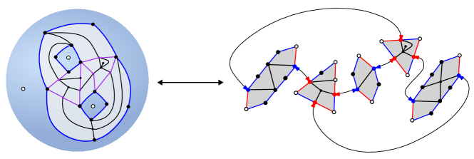
Figure 3: An example of a tight pair of pants, i.e. a planar map with three boundaries (in blue) of minimal length in their homotopy class in the triply punctured sphere. On the right the canonical decomposition described in [Bouttier_Bijective_2022]. Figure adapted from [Bouttier_Bijective_2022, Fig. 1.1].

Our result (28) for the genus-$0$ tight Weil–Petersson volumes with three distinguished boundaries can be seen as the analogue of [Bouttier_Bijective_2022, Theorem 1.1], although less powerful because our proof is not bijective. Instead, we derive generating functions of tight Weil–Petersson volumes from known expressions in the case of ordinary Weil–Petersson volumes. The general idea is that a genus-$0$ hyperbolic surface with two distinguished (but not necessarily tight) boundaries can unambiguously be cut along a shortest geodesic separating those two boundaries, resulting in a pair of certain half-tight cylinders (Figure 5). Also a genus-$g$ surface with $n$ distinguished (not necessarily tight) boundaries can be shown to decompose into a tight hyperbolic surface and $n$ half-tight cylinders. The first decomposition uniquely determines the Weil–Petersson volumes of the moduli spaces of half-tight cylinders, while the second determines the tight Weil–Petersson volumes. This relation is at the basis of Proposition 1.

To arrive at the recursion formula of Theorem 2 we follow the line or reasoning of Mirzakhani’s proof [Mirzakhani2007a] of Witten’s conjecture [Witten_Two_1991] (proved first by Kontsevich [Kontsevich1992]). She observes that the recursion equation (1) implies that the generating function of certain intersection numbers satisfies an infinite family of partial differential equations, the Virasoro constraints. Mulase & Safnuk [mulase2006mirzakhanis] have observed that the reverse implication is true as well. We will demonstrate that the generating functions of tight Weil–Petersson volumes and ordinary Weil–Petersson volumes are related in a simple fashion when expressed in terms of the times (14) and that the former obey a modified family of Virasoro constraints. These constraints in turn are equivalent to the generalized recursion of Theorem 2.

1.7 Discussion

Mirzakhani’s recursion formula has a bijective interpretation [Mirzakhani2007]. Upon multiplication by $2L_{1}$ the left-hand side $2L_{1}V_{g,n}(\mathbf{L})$ accounts for the volume of surfaces with a marked point on the first boundary. Tracing a geodesic ray from this point, perpendicularly to the boundary, until it self-intersects or hits another boundary allows one to canonically decompose the surface into a hyperbolic pair of pants (3-holed sphere) and one or two smaller hyperbolic surfaces. The terms on the right-hand side of [Mirzakhani2007] precisely take into account the Weil–Petersson volumes associated to these parts and the way they are glued.

It is natural to expect that Theorem 2 admits a similar bijective interpretation, in which the surface decomposes into a tight pair of pants (a sphere with $3+p$ boundaries, three of which are tight) and one or two smaller tight hyperbolic surfaces. However, Mirzakhani’s ray shooting procedure does not generalize in an obvious way. Nevertheless, working under the assumption that a bijective decomposition exists, one is led to suspect that the generalized kernel $K(x,t,\mu]$ of Theorem 2 contains important information about the geometry of tight pairs of pants. Moreover, one would hope that this geometry can be further understood via a decomposition of the tight pairs of pants themselves analogous to the planar map case of [Bouttier_Bijective_2022] described above.

Since a genus-$0$ surface $\mathsf{X}\in\mathcal{M}_{0,3+p}(0,0,0,\mathbf{L})$ with three distinguished cusps is always a tight pair of pants (since the zero length boundaries are obviously minimal), a consequence of a bijective interpretation of Theorem 2 is a conjectural interpretation of the series $\hat{X}(u;\mu]=\sin(2\pi u)/(2\pi u\eta)$ in (27) in terms of the hyperbolic distances between the three cusps. To be precise, let $c_{1},c_{2},c_{3}$ be unit-length horocycles around the three cusps and $\Delta(\mathsf{X})=d_{\mathrm{hyp}}(c_{1},c_{2})-d_{\mathrm{hyp}}(c_{1},c_{3})$ the difference in hyperbolic distance between two pairs, then it is plausible that

$$\hat{X}(u;\mu]\stackrel{{\scriptstyle?}}{{=}}\sum_{p\geq 0}\frac{1}{p!}\int\left(\int_{\mathcal{M}_{0,3+p}(0,0,0,\mathbf{L})}e^{2u\Delta(\mathsf{X})}\mathrm{d}\mu_{\mathrm{WP}}(\mathsf{X})\right)\mathrm{d}\mu(L_{1})\cdots\mathrm{d}\mu(L_{p}).$$ (43)

Or in the probabilistic terms of Section 1.3, the measure $M_{0}[\mu]X(z;\mu]$ on $\mathbb{R}$, which integrates to $1$ due to (28), is the probability distribution of the random variable $2\Delta(\mathsf{X})$ in a genus-$0$ Boltzmann hyperbolic surface $\mathsf{X}$ with weight $\mu$. In upcoming work we shall address this conjecture using very different methods.

Another natural question to ask is whether the generalization of the spectral curve (6) of Weil–Petersson volumes to the one of tight Weil–Petersson volumes in Theorem 3 can be understood in the general framework of deformations of spectral curves in topological recursion [Eynard_Invariants_2007].

1.8 Outline

The structure of the paper is as follows:

In section 2 we introduce the half-tight cylinder, which allows us to do tight decomposition of surfaces, which relates the regular hyperbolic surfaces to the tight surfaces. Using the decomposition we prove Proposition 1.

In section 3 consider the generating functions of (tight) Weil–Petersson volumes and their relations. Furthermore, we use the Virasoro constraints to prove Theorem 2, Theorem 4 and Corollary 5.

In section 4 we take the Laplace transform of the tight Weil–Petersson volumes and prove Theorem 3. We also look at the relation between the disk function of the regular hyperbolic surfaces and the generating series of moment $\eta$.

Finally, in section LABEL:sec:JT we briefly discuss how our results may be of use in the study of JT gravity.

Acknowledgments

This work is supported by the START-UP 2018 programme with project number 740.018.017 and the VIDI programme with project number VI.Vidi.193.048, which are financed by the Dutch Research Council (NWO).

2 Decomposition of tight hyperbolic surfaces

2.1 Half-tight cylinder

Recall that a boundary $\partial_{i}$ of $X\in\mathcal{M}_{g,n+p}(\mathbf{L})$ is said to be tight in $\invbreve{S}_{g,n,p}$ if $\partial_{i}$ is the only simple cycle $\gamma$ in $[\partial_{i}]_{\invbreve{S}_{g,n,p}}$ of length $\ell_{\gamma}(X)\leq L_{i}$ and we defined the moduli space of tight hyperbolic surfaces as

$$\mathcal{M}^{\text{tight}}_{g,n,p}(\mathbf{L}) =\{X\in\mathcal{M}_{g,n+p}(\mathbf{L}):\partial_{i}\text{ is tight in }\invbreve{S}_{g,n,p}\}\subset\mathcal{M}_{g,n+p}(\mathbf{L}).$$ (44)

We noted before that when $g=0$ and $n=2$ we have $\mathcal{M}^{\text{tight}}_{0,2,p}(\mathbf{L})=\emptyset$ because $\partial_{1}$ and $\partial_{2}$ belong to the same free homotopy class of $\invbreve{S}_{0,2,p}$ and can therefore never both be the unique shortest cycle. Instead, it is useful for any $p\geq 1$ to consider the moduli space of half-tight cylinders

$$\mathcal{H}_{p}(\mathbf{L}) =\{X\in\mathcal{M}_{0,2+p}(\mathbf{L}):\partial_{2}\text{ is tight in }\invbreve{S}_{0,2,p}\}\subset\mathcal{M}_{0,2+p}(\mathbf{L}),$$ (45)

which is non-empty whenever $L_{1}>L_{2}>0$. We will also consider

$$\overline{\mathcal{H}_{p}}(\mathbf{L}) =\{X\in\mathcal{M}_{0,2+p}(\mathbf{L}):\partial_{2}\text{ has minimal length in }[\partial_{2}]_{\invbreve{S}_{0,2,p}}\}\subset\mathcal{M}_{0,2+p}(\mathbf{L})$$ (46)

and denote its Weil–Petersson volume by $H_{p}(\mathbf{L})$. By construction, it is non-zero for $L_{1}\geq L_{2}>0$ and $H_{p}(\mathbf{L})\leq V_{0,2+p}(\mathbf{L})$.

Lemma 6.

$\mathcal{H}_{p}(\mathbf{L})$ is an open subset of $\mathcal{M}_{0,2+p}(\mathbf{L})$, and when it is non-empty ($L_{1}>L_{2}$) its closure is $\overline{\mathcal{H}_{p}}(\mathbf{L})$. In particular, both have the same finite Weil–Petersson volume $H_{p}(\mathbf{L})$ when $L_{1}>L_{2}$, but $\mathcal{H}_{p}(\mathbf{L})$ has $0$ volume and $\overline{\mathcal{H}_{p}}(\mathbf{L})$ non-zero volume $H_{p}(\mathbf{L})$ when $L_{1}=L_{2}$.

Proof.

For $L_{1}>L_{2}$, $\mathcal{H}_{p}(\mathbf{L})$ is the intersection of the open sets $\{\ell_{\gamma}(X)>L_{2}\}$ indexed by the countable set of free homotopy classes $\gamma$ in $[\partial_{2}]_{\invbreve{S}_{0,2,p}}$. It is not hard to see that in a neighbourhood of any $X\in\mathcal{H}_{p}(\mathbf{L})$ only finitely many of these are important, so the intersection is open. Its closure is given by the countable intersection of closed sets $\{\ell_{\gamma}(X)\geq L_{2}\}$, which is precisely $\overline{\mathcal{H}_{p}}(\mathbf{L})$. ∎

2.2 Tight decomposition

We are now ready to state the main result of this section.

Proposition 7.

The Weil–Petersson volumes $T_{g,n,p}(\mathbf{L})$ and $H_{p}(\mathbf{L})$ satisfy

$$V_{g,n+p}(\mathbf{L}) =\sum_{I_{0}\sqcup\cdots\sqcup I_{n}=\{n+1,\ldots,n+p\}}\int T_{g,n,|I_{0}|}(\mathbf{K},\mathbf{L}_{I_{0}})\prod_{\begin{subarray}{c}1\leq i\leq n\\ I_{i}\neq\emptyset\end{subarray}}H_{|I_{i}|}(L_{i},K_{i},\mathbf{L}_{I_{i}})\,K_{i}\mathrm{d}K_{i},\qquad(g\geq 1\text{ or }n\geq 3)$$

$$V_{0,2+p}(\mathbf{L}) =H_{p}(\mathbf{L})+\sum_{\begin{subarray}{c}I_{1}\sqcup I_{2}=\{3,\ldots,2+p\}\\ I_{1},I_{2}\neq\emptyset\end{subarray}}\int_{0}^{L_{2}}H_{|I_{1}|}(L_{1},K,\mathbf{L}_{I_{1}})H_{|I_{2}|}(L_{2},K,\mathbf{L}_{I_{2}})K\mathrm{d}K,\qquad(L_{1}\geq L_{2})$$

where in the first equation it is understood that $K_{i}=L_{i}$ whenever $I_{i}=\emptyset$.

The remainder of this section will be devoted to proving this result. But let us first see how it implies Proposition 1.

Proof of Proposition 1.

Clearly $H_{1}(\mathbf{L})=V_{0,3}(\mathbf{L})=1$ for $L_{1}\geq L_{2}$ and $T_{g,n,0}(\mathbf{L})=V_{g,n}(\mathbf{L})$. Rewriting the equations as

$$T_{g,n,p}(\mathbf{L}) =V_{g,n+p}(\mathbf{L})-\sum_{\begin{subarray}{c}I_{0}\sqcup\cdots\sqcup I_{n}=\{n+1,\ldots,n+p\}\\ |I_{0}|<p\end{subarray}}\int T_{g,n,|I_{0}|}(\mathbf{K},\mathbf{L}_{I_{0}})\prod_{\begin{subarray}{c}1\leq i\leq n\\ I_{i}\neq\emptyset\end{subarray}}H_{|I_{i}|}(L_{i},K_{i},\mathbf{L}_{I_{i}})\,K_{i}\mathrm{d}K_{i},$$

$$H_{p}(\mathbf{L}) =V_{0,2+p}(\mathbf{L})-\sum_{\begin{subarray}{c}I_{1}\sqcup I_{2}=\{3,\ldots,2+p\}\\ I_{1},I_{2}\neq\emptyset\end{subarray}}\int_{0}^{L_{2}}H_{|I_{1}|}(L_{1},K,\mathbf{L}_{I_{1}})H_{|I_{2}|}(L_{2},K,\mathbf{L}_{I_{2}})K\mathrm{d}K,$$

it is clear that they are uniquely determined recursively in terms of $V_{g,n}(\mathbf{L})$. Moreover, by induction we easily verify that $H_{p}(\mathbf{L})$ in the region $L_{1}\geq L_{2}$ is a polynomial in $L_{1}^{2},\ldots,L_{2+p}^{2}$ of degree $p-1$ that is symmetric in $L_{3},\ldots,L_{2+p}$, and $T_{g,n,p}$ is a polynomial in $L_{1}^{2},\ldots,L_{n+p}^{2}$ of degree $3g-3+n+p$ that is symmetric in $L_{1},\ldots,L_{n}$ and symmetric in $L_{n+1},\ldots,L_{n+p}$. ∎

2.3 Tight decomposition in the stable case

2.3.1 Shortest cycles

The following parallels the construction of shortest cycles in maps described in [Bouttier_Bijective_2022, Section 6.1].

Lemma 8.

Given a hyperbolic surface $X\in\mathcal{M}_{g,n+p}$ for $g\geq 1$ or $n\geq 2$, then for each $i=1,\ldots,n$ there exists a unique innermost shortest cycle $\sigma^{i}_{\invbreve{S}_{g,n,p}}(X)$ on $X$, meaning that it has minimal length in $[\partial_{i}]_{\invbreve{S}_{g,n,p}}$ and such that all other cycles of minimal length (if they exist) are contained in the region of $X$ delimited by $\partial_{i}$ and $\sigma^{i}_{\invbreve{S}_{g,n,p}}(X)$. Moreover, if $g\geq 1$ or $n\geq 3$, the curves $\sigma^{1}_{\invbreve{S}_{g,n,p}}(X),\ldots,\sigma^{n}_{\invbreve{S}_{g,n,p}}(X)$ are disjoint.

Proof.

First note that if a shortest cycle exists, it is a simple closed geodesic. As a consequence of [buser1992geometry, Theorem 1.6.11], there are only finitely many closed geodesics with length $\leq L_{i}$ in $[\partial_{i}]_{\invbreve{S}_{g,n,p}}$. Since $\partial_{i}\in[\partial_{i}]_{\invbreve{S}_{g,n,p}}$ has length $L_{i}$, this proves the existence of at least one cycle in $[\partial_{i}]_{\invbreve{S}_{g,n,p}}$ with minimal length.

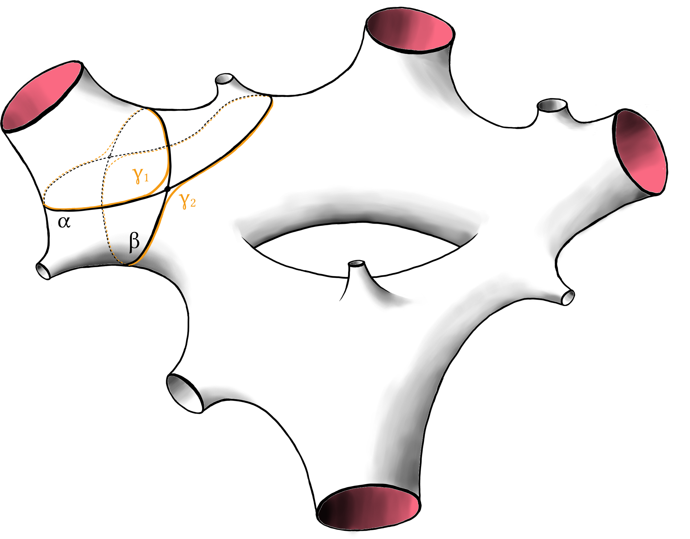
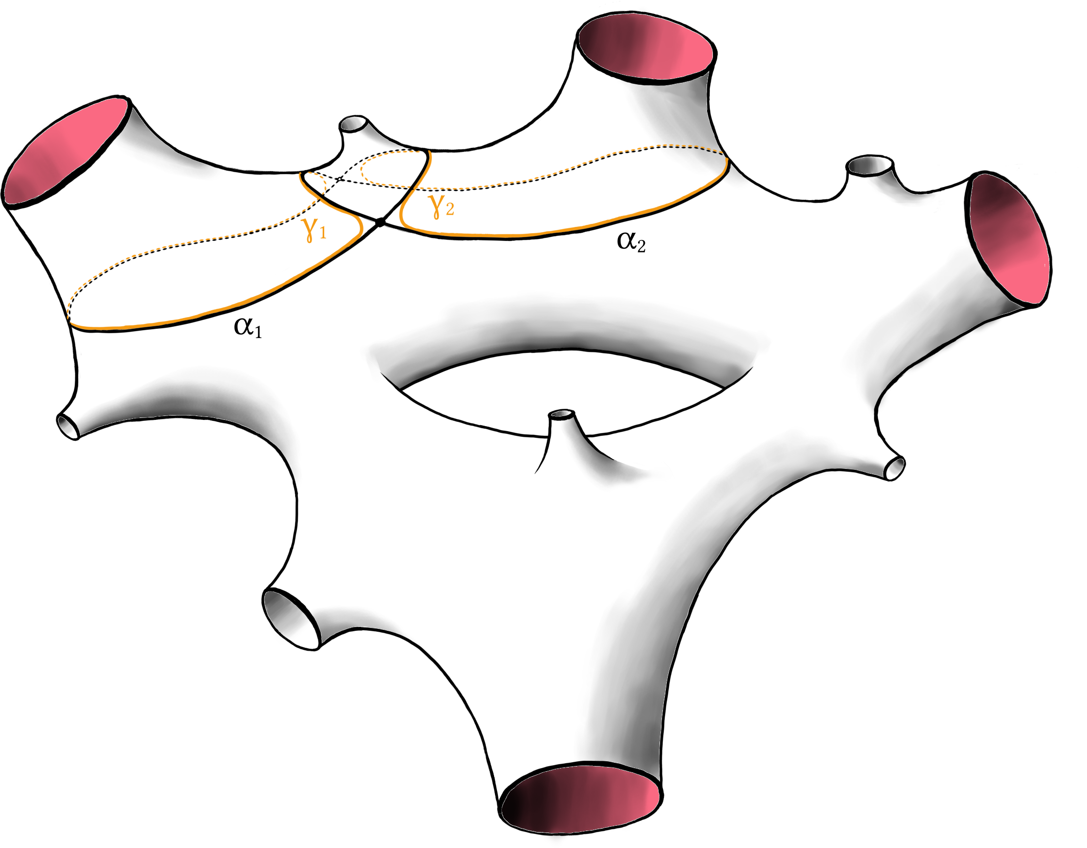
Figure 4: Illustrations of why two intersecting geodesics $\alpha$ and $\beta$ cannot both have minimal length in their free-homotopy classes on $\invbreve{S}_{g,n,p}$.

Regarding the existence and uniqueness of a well-defined innermost shortest cycle, suppose $\alpha,\beta\in[\partial_{i}]_{\invbreve{S}_{g,n,p}}$ are two distinct simple closed geodesics with minimal length $\ell$ (see left side of Figure 4). Since $\alpha\in[\partial_{i}]_{\invbreve{S}_{g,n,p}}$, cutting along $\alpha$ separates the surface in two disjoint parts. Therefore, $\alpha$ and $\beta$ can only have an even number of intersections. If the number of intersections is greater than zero, we can choose two distinct intersections and combine $\alpha$ and $\beta$ to get two distinct cycles $\gamma_{1}$ and $\gamma_{2}$ by switching between $\alpha$ and $\beta$ at the chosen intersections, such that $\gamma_{1}$ and $\gamma_{2}$ are still in $[\partial_{i}]_{\invbreve{S}_{g,n,p}}$. Since the total length is still $2\ell$, at least one of the new cycles has length $\leq\ell$. This cycle is not geodesic, so there will be a closed cycle in $[\partial_{i}]_{\invbreve{S}_{g,n,p}}$ with length $<\ell$, which contradicts that $\alpha$ and $\beta$ have minimal length. We conclude that $\alpha$ and $\beta$ are disjoint. Since all cycles in $[\partial_{i}]_{\invbreve{S}_{g,n,p}}$ with minimal length are disjoint and separating, the notion of being innermost is well-defined.

Consider $\alpha_{i}=\sigma^{i}_{\invbreve{S}_{g,n,p}}(X)$ and $\alpha_{j}=\sigma^{j}_{\invbreve{S}_{g,n,p}}(X)$ for $i\neq j$ (see right side of Figure 4). Just as before, since $\alpha_{i}$ is separating and $\alpha_{i}$ and $\alpha_{j}$ are simple, the number of intersections is even. If $\alpha_{i}$ and $\alpha_{j}$ are not disjoint, we can choose two distinct intersections and construct two distinct cycles $\gamma_{i}$ and $\gamma_{j}$ by switching between $\alpha_{i}$ and $\alpha_{j}$ at the chosen intersections, such that $\gamma_{i}$ and $\gamma_{j}$ are in $[\partial_{i}]_{\invbreve{S}_{g,n,p}}$ and $[\partial_{j}]_{\invbreve{S}_{g,n,p}}$ respectively. Since the total length of the cycles stays the same, there is at least one $a\in\{i,j\}$ such that $\gamma_{a}$ has length less or equal than $\alpha_{a}$. Since $\gamma_{a}$ is not geodesic, there is a closed cycle in $[\partial_{a}]_{\invbreve{S}_{g,n,p}}$ with length strictly smaller than $\alpha_{a}$, which is a contradiction, so the innermost shortest cycles are disjoint. ∎

In particular the proof implies the following criterions are equivalent:

• A simple closed geodesic $\alpha\in[\partial_{i}]_{\invbreve{S}_{g,n,p}}$ is the innermost shortest cycle $\sigma^{i}_{\invbreve{S}_{g,n,p}}(X)$;

• For a simple closed geodesic $\alpha\in[\partial_{i}]_{\invbreve{S}_{g,n,p}}$ we have $\ell(\alpha)\leq L_{i}$ and each simple closed geodesic $\beta\in\sigma^{i}_{\invbreve{S}_{g,n,p}}(X)$ that is disjoint from $\alpha$ has length $\ell(\beta)\geq\ell(\alpha)$ with equality only being allowed if $\beta$ is contained in the region between $\alpha$ and $\partial_{i}$.

2.3.2 Integration on Moduli space

Let us recap Mirzakhani’s decomposition of moduli space integrals in the presence of distinguished cycles [Mirzakhani2007, Section 8]. A multicurve $\Gamma=(\gamma_{1},\ldots,\gamma_{k})$ is a collection of disjoint simple closed curves $\Gamma=(\gamma_{1},\ldots,\gamma_{k})$ in $S_{g,n}$ which are pairwise non-freely-homotopic. Given a multicurve, in which each curve $\gamma_{i}$ may or may not be freely homotopic to a boundary $\partial_{j}$ of $S_{g,n}$, one can consider the stabilizer subgroup

$$\operatorname{Stab}(\Gamma)=\{h\in\mathrm{Mod}_{g,n}:h\cdot\gamma_{i}=\gamma_{i}\}\subset\mathrm{Mod}_{g,n}.$$

Note that if $\gamma_{i}\in[\partial_{j}]_{S_{g,n}}$ is freely homotopic to one of the boundaries $\partial_{j}$ then $h\cdot\gamma_{i}=\gamma_{i}$ for any $h\in\mathrm{Mod}_{g,n}$. The moduli space of hyperbolic surfaces with distinguished (free homotopy classes of) curves is the quotient

$$\mathcal{M}_{g,n}(\mathbf{L})^{\Gamma}=\mathcal{T}_{g,n}(\mathbf{L})/\operatorname{Stab}(\Gamma).$$

For a closed curve $\gamma$ in $S_{g,n}$ and $X\in\mathcal{M}_{g,n}$, let $\ell_{\gamma}(X)$ be the length of the geodesic representative in the free homotopy class of $\gamma$. For $\mathbf{K}=(K_{1},\ldots,K_{k})\subset\mathbb{R}_{>0}^{k}$ we can restrict the lengths of the geodesic representatives of curves in $\Gamma$ by setting

$$\mathcal{M}_{g,n}(\mathbf{L})^{\Gamma}(\mathbf{K})=\{X\in\mathcal{M}_{g,n}(\mathbf{L})^{\Gamma}:\ell_{\gamma_{i}}(X)=K_{i},i=1,\ldots,k\}\subset\mathcal{M}_{g,n}(\mathbf{L})^{\Gamma}.$$

If $\gamma_{i}\in[\partial_{j}]_{S_{g,n}}$ then this set is empty unless $K_{i}=L_{j}$. Denote by $\pi^{\Gamma}:\mathcal{M}_{g,n}(\mathbf{L})^{\Gamma}\to\mathcal{M}_{g,n}(\mathbf{L})$ the projection. If there are exactly $p$ cycles among $\Gamma$ that are not freely homotopic to a boundary, then this space admits a natural action of the $p$-dimensional torus $(S^{1})^{p}$ obtained by twisting along each of these $p$ cycles proportional to their length. The quotient space is denoted

$$\mathcal{M}_{g,n}(\mathbf{L})^{\Gamma*}(\mathbf{K})=\mathcal{M}_{g,n}(\mathbf{L})^{\Gamma}(\mathbf{K})/(S^{1})^{p}$$

and is naturally equipped with a symplectic structure inherited from the Weil–Petersson symplectic structure on $\mathcal{M}_{g,n}(\mathbf{L})^{\Gamma}$. If we denote by $S_{g,n}(\Gamma)$ the possibly disconnected surface obtained from $S_{g,n}$ by cutting along all $\gamma_{i}$ that are not freely homotopic to a boundary and by $\mathcal{M}(S_{g,n}(\Gamma),\mathbf{L},\mathbf{K})$ its moduli space, then according to [Mirzakhani2007, Lemma 8.3], the canonical mapping

$$\mathcal{M}_{g,n}(\mathbf{L})^{\Gamma*}(\mathbf{K})\to\mathcal{M}(S_{g,n}(\Gamma),\mathbf{L},\mathbf{K})$$ (47)

is a symplectomorphism. Given an integrable function $F:\mathcal{M}_{g,n}(\mathbf{L})^{\Gamma}\to\mathbb{R}$ that is invariant under the action of $(S^{1})^{p}$, there exists a naturally associated function $\tilde{F}:\mathcal{M}(S_{g,n}(\Gamma),\mathbf{L},\mathbf{K})\to\mathbb{R}$ such that (essentially [Mirzakhani2007, Lemma 8.4])

$$\int_{\mathcal{M}_{g,n}(\mathbf{L})^{\Gamma}}F(X)\mathrm{d}\mu_{WP}(X)=\int\prod_{\begin{subarray}{c}1\leq i\leq n\\ \gamma_{i}\notin[\partial_{j}]_{S_{g,n}}\end{subarray}}K_{i}\mathrm{d}K_{i}\int_{\mathcal{M}(S_{g,n}(\Gamma),\mathbf{L},\mathbf{K})}\tilde{F}(X)\mathrm{d}\mu_{WP}(X).$$ (48)

2.3.3 Shortest multicurves

Suppose $g\geq 1$ or $n\geq 3$, meaning that we momentarily exclude the cylinder case ($g=0$, $n=2$). We consider now a special family of multicurves $\Gamma=(\gamma_{1},\ldots,\gamma_{n})$ on $S_{g,n+p}$ for $n\geq 1,p\geq 0$. Namely, we require that $\gamma_{i}\in[\partial_{i}]_{\invbreve{S}_{g,n,p}}$ is freely homotopic to the boundary $\partial_{i}$ in the capped-off surface $\invbreve{S}_{g,n,p}$ for $i=1,\ldots,n$. Then there exists a partition $I_{0}\sqcup\cdots\sqcup I_{n}=\{n+1,\ldots,n+p\}$ such that $S_{g,n+p}(\Gamma)$ has $n+1$ connected components $s_{0},\ldots,s_{n}$, where $s_{0}$ is of genus $g$ and is adjacent to all curves $\Gamma$ as well as the boundaries $(\partial_{j})_{j\in I_{0}}$ while for each $i=1,\ldots,n$, $s_{i}$ is of genus $0$ and contains the $i$th boundary $\partial_{i}$ as well as $(\partial_{j})_{j\in I_{i}}$ and is adjacent to $\gamma_{i}$. Note that $I_{i}=\emptyset$ if and only if $\gamma_{i}\in[\partial_{i}]_{S_{g,n+p}}$. Finally, we observe that mapping class group orbits $\{\text{Mod}_{g,n+p}\cdot[\Gamma]_{S_{g,n+p}}\}$ of these multicurves $\Gamma$ are in bijection with the set of partitions $\{I_{0}\sqcup\cdots\sqcup I_{n}=\{n+1,\ldots,n+p\}\}$.

With the help of Lemma 8 we may introduce the restricted moduli space in which we require $\gamma_{i}$ to be (freely homotopic to) the innermost shortest cycle in $[\partial_{i}]_{\invbreve{S}_{g,n,p}}$,

$$\hat{\mathcal{M}}_{g,n,p}(\mathbf{L})^{\Gamma}=\left\{X\in\mathcal{M}_{g,n+p}(\mathbf{L})^{\Gamma}:\gamma_{i}\in[\sigma^{i}_{\invbreve{S}_{g,n,p}}(X)]\text{ for }i=1,\ldots,n\right\}.$$

Lemma 9.

The natural projection

$$\bigsqcup_{\Gamma}\hat{\mathcal{M}}_{g,n,p}(\mathbf{L})^{\Gamma}\longrightarrow\mathcal{M}_{g,n+p}(\mathbf{L}),$$

where the disjoint union is over (representatives of) the mapping class group orbits of multicurves $\Gamma$, is a bijection.

Proof.

If $X,X^{\prime}\in\mathcal{T}_{g,n+p}(\mathbf{L})$ are representatives of hyperbolic surfaces in $\hat{\mathcal{M}}_{g,n,p}(\mathbf{L})^{\Gamma}$ and $\hat{\mathcal{M}}_{g,n,p}(\mathbf{L})^{\Gamma^{\prime}}$ respectively, then by definition $[\gamma_{i}]=[\sigma^{i}_{\invbreve{S}_{g,n,p}}(X)]$ and $[\gamma_{i}^{\prime}]=[\sigma^{i}_{\invbreve{S}_{g,n,p}}(X^{\prime})]$. If $X$ and $X^{\prime}$ represent the same surface in $\mathcal{M}_{g,n+p}(\mathbf{L})$, they are related by an element $h$ of the mapping class group, $X^{\prime}=h\cdot X$, and therefore also $\sigma^{i}_{\invbreve{S}_{g,n,p}}(X)=h\cdot\sigma^{i}_{\invbreve{S}_{g,n,p}}(X^{\prime})$ and $[\gamma_{i}]=h\cdot[\gamma_{i}^{\prime}]$. So $\Gamma$ and $\Gamma^{\prime}$ belong to the same mapping class group orbit and, if $\Gamma$ and $\Gamma^{\prime}$ are freely homotopic, we must have $h\in\operatorname{Stab}(\Gamma)$. Hence, $X$ and $X^{\prime}$ represent the same element in the set on the left-hand side, and we conclude that the projection is injective. It is also surjective since any $X\in\mathcal{T}_{g,n+p}(\mathbf{L})$ is a representative of $\hat{\mathcal{M}}_{g,n,p}(\mathbf{L})^{\Gamma}$ if we take $\Gamma=(\sigma^{1}_{\invbreve{S}_{g,n,p}}(X),\ldots,\sigma^{n}_{\invbreve{S}_{g,n,p}}(X))$, which is a valid multicurve due to Lemma 8. ∎

We can introduce the length-restricted version $\hat{\mathcal{M}}_{g,n,p}(\mathbf{L})^{\Gamma}(\mathbf{K})\subset\mathcal{M}_{g,n+p}(\mathbf{L})^{\Gamma}(\mathbf{K})$ as before.

Lemma 10.

The subset $\hat{\mathcal{M}}_{g,n,p}(\mathbf{L})^{\Gamma}(\mathbf{K})\subset\mathcal{M}_{g,n+p}(\mathbf{L})^{\Gamma}(\mathbf{K})$ is invariant under twisting (the torus-action on $\mathcal{M}_{g,n+p}(\mathbf{L})^{\Gamma}(\mathbf{K})$ described above). The image of the quotient $\hat{\mathcal{M}}_{g,n,p}(\mathbf{L})^{\Gamma*}(\mathbf{K})$ under the symplectomorphism (47) is precisely

$$\mathcal{M}^{\text{tight}}_{g,n,|I_{0}|}(\mathbf{K},\mathbf{L}_{I_{0}})\times\prod_{\begin{subarray}{c}1\leq i\leq n\\ I_{i}\neq\emptyset\end{subarray}}\overline{\mathcal{H}_{|I_{i}|}}(L_{i},K_{i},\mathbf{L}_{I_{i}}).$$ (49)

Proof.

Let $X\in\mathcal{M}_{g,n+p}(\mathbf{L})^{\Gamma}(\mathbf{K})$ be a hyperbolic surface with distinguished multicurve $\Gamma$. The lengths of the geodesics associated to $\Gamma$ as well as the lengths of the geodesics that are disjoint from those geodesics are invariant under twisting $X$ along $\Gamma$. The criterion explained just below Lemma 8 for $\gamma_{i}$ to be the innermost shortest cycle $\sigma^{i}_{\invbreve{S}_{g,n,p}}(X)$ is thus also preserved under twisting, showing that the subset $\hat{\mathcal{M}}_{g,n,p}(\mathbf{L})^{\Gamma}(\mathbf{K})$ is invariant.

Let $X_{0}\in\mathcal{M}_{g,n,|I_{0}|}(\mathbf{K},\mathbf{L}_{I_{0}})$ and $X_{i}\in\mathcal{M}_{0,2+|I_{i}|}(L_{i},K_{i},\mathbf{L}_{I_{i}})$ for those $i=1,\ldots,n$ for which $I_{i}\neq\emptyset$ be the hyperbolic structures on the connected components $s_{0},\ldots,s_{n}$ of $S_{g,n+p}(\Gamma)$ obtained by cutting $X$ along the geodesics associated to $\Gamma$. For each $i=1,\ldots,n$ the criterion for $\gamma_{i}$ to be the innermost shortest cycle $\sigma^{i}_{\invbreve{S}_{g,n,p}}(X)$ is equivalent to the following two conditions holding:

• the $i$th boundary of $X_{0}$ is tight in the capped-off surface associated to $s_{0}$;

• $I_{i}=\emptyset$ (meaning $\gamma_{i}=\partial_{i}$) or $X_{i}\in\overline{\mathcal{H}_{|I_{i}|}}(L_{i},K_{i},\mathbf{L}_{I_{i}})$ (recall the definition in (46)).

Hence, we have $X\in\hat{\mathcal{M}}_{g,n,p}(\mathbf{L})^{\Gamma}(\mathbf{K})$ precisely when $X_{0}\in\mathcal{M}^{\text{tight}}_{g,n,|I_{0}|}(\mathbf{K},\mathbf{L}_{I_{0}})$ and $X_{i}\in\overline{\mathcal{H}_{|I_{i}|}}(L_{i},K_{i},\mathbf{L}_{I_{i}})$ when $I_{i}\neq\emptyset$. This proves the second statement of the lemma. ∎

It follows that the Weil–Petersson volume of $\hat{\mathcal{M}}_{g,n,p}(\mathbf{L})^{\Gamma*}(\mathbf{K})$ is equal to the product of the volumes of the spaces appearing in (49). Combining with Lemma 9 and the integration formula (48) this shows that

$$V_{g,n+p}(\mathbf{L}) =\sum_{\Gamma}\int_{\hat{\mathcal{M}}_{g,n,p}(\mathbf{L})^{\Gamma}}\mathrm{d}\mu_{WP}$$

$$=\sum_{I_{0}\sqcup\cdots\sqcup I_{n}=\{n+1,\ldots,n+p\}}\int T_{g,n,|I_{0}|}(\mathbf{K},\mathbf{L}_{I_{0}})\prod_{\begin{subarray}{c}1\leq i\leq n\\ I_{i}\neq\emptyset\end{subarray}}H_{|I_{i}|}(L_{i},K_{i},\mathbf{L}_{I_{i}})\,K_{i}\mathrm{d}K_{i},$$

where it is understood that $K_{i}=L_{i}$ whenever $I_{i}=\emptyset$. This proves the first relation of Proposition 7.

2.4 Tight decomposition of the cylinder

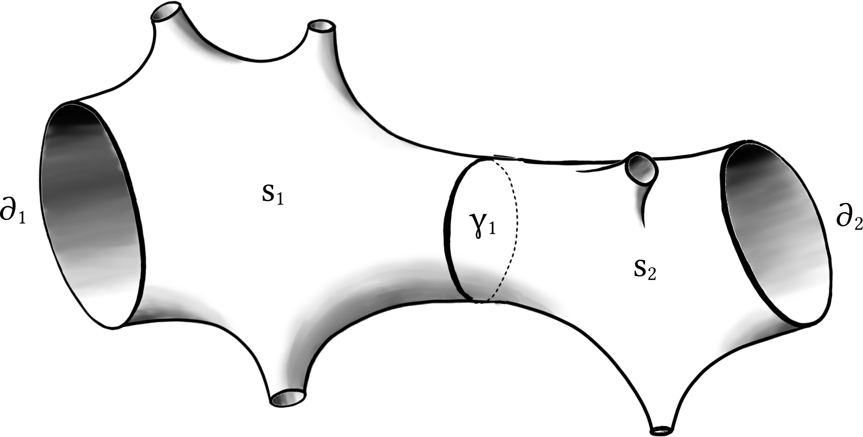
Figure 5: A surface with two distinguished boundaries $\partial_{1}$ and $\partial_{2}$ naturally decomposes into a pair of half-tight cylinders.

The decomposition we have just described does not work well in the case $g=0$ and $n=2$, because $\partial_{1}$ and $\partial_{2}$ are in the same free homotopy class of the capped surface $\invbreve{S}_{0,2,p}$. Instead, we should consider a multicurve $\Gamma=(\gamma_{1})$ consisting of a single curve $\gamma_{1}$ on $S_{0,2+p}$ in the free homotopy class $[\partial_{1}]_{\invbreve{S}_{0,2,p}}=[\partial_{2}]_{\invbreve{S}_{0,2,p}}$, see Figure 5. In this case there exists a partition $I_{1}\sqcup I_{2}=\{3,\ldots,p+2\}$ such that $S_{0,2+p}(\Gamma)$ has two connected components $s_{1}$ and $s_{2}$, with $s_{i}$ a genus-$0$ surface with $2+|I_{i}|$ boundaries corresponding to $\partial_{i}$, $\gamma_{1}$ and $(\partial_{j})_{j\in I_{i}}$. We consider the restricted moduli space

$$\hat{\mathcal{M}}_{0,2,p}(\mathbf{L})^{\Gamma}=\left\{X\in\mathcal{M}_{0,2+p}(\mathbf{L})^{\Gamma}:\gamma_{1}\in[\sigma^{1}_{\invbreve{S}_{0,2,p}}(X)]\right\},$$

which thus treats the two boundaries $\partial_{1}$ and $\partial_{2}$ asymmetrically, by requiring that $\gamma_{1}$ is the shortest curve farthest from $\partial_{1}$. Lemma 9 goes through unchanged: the projection

$$\bigsqcup_{\Gamma}\hat{\mathcal{M}}_{0,2,p}(\mathbf{L})^{\Gamma}\longrightarrow\mathcal{M}_{0,2+p}(\mathbf{L}),$$

where the disjoint union is over the mapping class group orbits of $\Gamma=(\gamma_{1})$, is a bijection. Assuming $L_{1}\geq L_{2}$, we cannot have $\gamma_{1}\in[\partial_{1}]_{S_{0,2+p}}$ so $I_{1}\neq\emptyset$. There are two cases to consider:

• $\gamma_{1}\in[\partial_{2}]_{S_{0,2+p}}$ and therefore $I_{2}=\emptyset$: this means that $\partial_{2}$ has minimal length in $[\partial_{2}]_{\invbreve{S}_{0,2,p}}$, so $\hat{\mathcal{M}}_{0,2,p}(\mathbf{L})^{\Gamma}=\overline{\mathcal{H}_{p}}(\mathbf{L})$.

• $I_{2}\neq\emptyset$: by reasoning analogous to that of Lemma 10 we have that $\hat{\mathcal{M}}_{0,2,p}(\mathbf{L})^{\Gamma*}(K)$ is symplectomorphic to

  $$\overline{\mathcal{H}_{|I_{1}|}}(L_{1},K,\mathbf{L}_{I_{1}})\times\mathcal{H}_{|I_{2}|}(L_{2},K,\mathbf{L}_{I_{2}}).$$

Hence, when $L_{1}\geq L_{2}$ we have

$$V_{0,2+p}(\mathbf{L}) =H_{p}(\mathbf{L})+\sum_{\begin{subarray}{c}I_{1}\sqcup I_{2}=\{3,\ldots,2+p\}\\ I_{1},I_{2}\neq\emptyset\end{subarray}}\int_{0}^{L_{2}}H_{|I_{1}|}(L_{1},K,\mathbf{L}_{I_{1}})H_{|I_{2}|}(L_{2},K,\mathbf{L}_{I_{2}})K\mathrm{d}K.$$

This proves the second relation of Proposition 7.

3 Generating functions of tight Weil–Petersson volumes

3.1 Definitions

Let us define the following generating functions of the Weil–Petersson volumes, half-tight cylinder volumes and tight Weil–Petersson volumes:

$$F_{g}[\mu] =\sum_{n=0}^{\infty}\frac{1}{n!}\int\differential{\mu(L_{1})}\cdots\int\differential{\mu(L_{n})}V_{g,n}(\mathbf{L}),$$ (50)

$$H(L_{1},L_{2};\mu] =\sum_{p=1}^{\infty}\frac{1}{p!}\int\differential{\mu(L_{3})}\cdots\int\differential{\mu(L_{2+p})}H_{p}(\mathbf{L}),$$ (51)

$$\tilde{F}_{g}[\nu,\mu] =\sum_{n=0}^{\infty}\frac{1}{n!}\int\differential{\nu(L_{1})}\cdots\int\differential{\nu(L_{n})}T_{g,n}(L_{1},\ldots,L_{n};\mu].$$ (52)

Furthermore, for $g\geq 2$ we recall the polynomial

$$\mathcal{P}_{g,0}(m_{1},\ldots,m_{3g-3})=\sum_{\begin{subarray}{c}d_{2},d_{3},\ldots\geq 0\\ \sum_{k\geq 2}(k-1)d_{k}=3g-3\end{subarray}}\!\!\!\!\langle\tau_{2}^{d_{2}}\tau_{3}^{d_{3}}\cdots\rangle_{g}\prod_{k\geq 2}\frac{(-m_{k-1})^{d_{k}}}{d_{k}!},$$ (53)

where $\langle\tau_{2}^{d_{2}}\tau_{3}^{d_{3}}\cdots\rangle_{g}$ are the $\psi$-class intersection numbers on the moduli space $\mathcal{M}_{g,n}$ with $n=\sum_{k}d_{k}\leq 3g-3$ marked points. Then according to [budd2020irreducible, Theorem 3]

$$F_{0}[\mu] =\frac{1}{2}\int_{0}^{R}\!\!\!\mathrm{d}r\,Z(r;\mu]^{2},$$ (54)

$$F_{1}[\mu] =-\frac{1}{24}\log M_{0}[\mu],$$ (55)

$$F_{g}[\mu] =\frac{1}{\left(M_{0}[\mu]\right)^{2g-2}}\,\mathcal{P}_{g,0}\left(\frac{M_{1}[\mu]}{M_{0}[\mu]},\ldots,\frac{M_{3g-3}[\mu]}{M_{0}[\mu]}\right)\quad\text{for }g\geq 2.$$ (56)

In the genus-$0$ case we can take successive derivatives to find useful formulas for one, two or three distinguished boundaries of prescribed lengths,

$$\functionalderivative{F_{0}[\mu]}{\mu(L_{1})} =-\int_{0}^{R[\mu]}I_{0}(L_{1}\sqrt{2r})\,Z(r;\mu]\mathrm{d}r,,$$ (57)

$$\frac{\delta^{2}F_{0}[\mu]}{\delta\mu(L_{1})\delta\mu(L_{2})} =\int_{0}^{R[\mu]}I_{0}(L_{1}\sqrt{2r})\,I_{0}(L_{2}\sqrt{2r})\mathrm{d}r,$$ (58)

$$\frac{\delta^{3}F_{0}[\mu]}{\delta\mu(L_{1})\delta\mu(L_{2})\delta\mu(L_{3})} =\frac{1}{M_{0}[\mu]}\left[\prod_{i=1}^{3}I_{0}(L_{i}\sqrt{2R[\mu]})\right].$$ (59)

3.2 Volume of half-tight cylinder

The equations of Proposition 7 turn into the equations

$$\frac{\delta^{n}F_{g}[\mu]}{\delta\mu(L_{1})\cdots\delta\mu(L_{n})} =\int T_{g,n}(\mathbf{K};\mu]\prod_{i=1}^{n}(K_{i}H(L_{i},K_{i};\mu]+\delta(K_{i}-L_{i}))\mathrm{d}K_{i},\qquad(g\geq 1\text{ or }n\geq 3)$$ (60)

$$\frac{\delta^{2}F_{0}[\mu]}{\delta\mu(L_{1})\delta\mu(L_{2})} =H(L_{1},L_{2};\mu]+\int_{0}^{L_{2}}H(L_{1},K;\mu]H(L_{2},K;\mu]K\mathrm{d}K.\qquad(L_{1}\geq L_{2})$$ (61)

Let us focus on the last equation, which should determine $H(L_{1},L_{2};\mu]$ uniquely. The left-hand side depends on $\mu$ only through the quantity $R[\mu]$, and the dependence on $R$ is analytic,

$$\frac{\delta^{2}F_{0}[\mu]}{\delta\mu(L_{1})\delta\mu(L_{2})}=R+\frac{1}{4}(L_{1}^{2}+L_{2}^{2})R^{2}+\frac{1}{48}(L_{1}^{4}+4L_{1}^{2}L_{2}^{2}+L_{2}^{4})R^{3}+\cdots.$$

Hence, the same is true for $H(L_{1},L_{2};\mu]$ and one may easily calculate order by order in $R$ that

$$H(L_{1},L_{2};\mu]=R+\frac{1}{4}(L_{1}^{2}-L_{2}^{2})R^{2}+\frac{1}{48}(L_{1}^{2}-L_{2}^{2})^{2}R^{3}+\cdots.$$

This suggests that $H(L_{1},L_{2};\mu]$ depends on $L_{1}$ and $L_{2}$ only through the combination $L_{1}^{2}-L_{2}^{2}$. Let’s prove this.

Lemma 11.

The half-tight cylinder generating function satisfies

$$\left(\frac{1}{L_{1}}\frac{\partial}{\partial L_{1}}+\frac{1}{L_{2}}\frac{\partial}{\partial L_{2}}\right)H(L_{1},L_{2};\mu]=0,$$ (62)

and is therefore given by

$$H(L_{1},L_{2};\mu]=\sum_{\ell=0}^{\infty}\frac{2^{-\ell}R[\mu]^{\ell+1}}{\ell!(\ell+1)!}(L_{1}^{2}-L_{2}^{2})^{\ell}=\sqrt{\frac{2R[\mu]}{L_{1}^{2}-L_{2}^{2}}}I_{1}\left(\sqrt{L_{1}^{2}-L_{2}^{2}}\sqrt{2R[\mu]}\right)\qquad(L_{1}\geq L_{2}).$$ (63)

Proof.

By construction $H(L_{1},0;\mu]=\frac{\delta^{2}F_{0}[\mu]}{\delta\mu(L_{1})\delta\mu(0)}$ and the integral (58) with $L_{2}=0$ evaluates to

$$H(L_{1},0;\mu]=\frac{\delta^{2}F_{0}[\mu]}{\delta\mu(L_{1})\delta\mu(0)} =\frac{\sqrt{2R}}{L_{1}}I_{1}(L_{1}\sqrt{2R}).$$ (64)

The identity

$$\frac{\partial}{\partial r}\left(\frac{\sqrt{2r}}{L_{1}}I_{1}(L_{1}\sqrt{2r})\frac{\sqrt{2r}}{L_{2}}I_{1}(L_{2}\sqrt{2r})\right)=\left(\frac{1}{L_{1}}\frac{\partial}{\partial L_{1}}+\frac{1}{L_{2}}\frac{\partial}{\partial L_{2}}\right)I_{0}(L_{1}\sqrt{2r})\,I_{0}(L_{2}\sqrt{2r}),$$

which can be easily checked by calculating the derivatives, implies that

$$H(L_{1},0;\mu]H(L_{2},0;\mu]=\left(\frac{1}{L_{1}}\frac{\partial}{\partial L_{1}}+\frac{1}{L_{2}}\frac{\partial}{\partial L_{2}}\right)\frac{\delta^{2}F_{0}[\mu]}{\delta\mu(L_{1})\delta\mu(L_{2})}.$$

Hence, by (61) we find that

$$\left(\frac{1}{L_{1}}\frac{\partial}{\partial L_{1}}+\frac{1}{L_{2}}\frac{\partial}{\partial L_{2}}\right)H(L_{1},L_{2};\mu] =H(L_{1},0;\mu]H(L_{2},0;\mu]-\left(\frac{1}{L_{1}}\frac{\partial}{\partial L_{1}}+\frac{1}{L_{2}}\frac{\partial}{\partial L_{2}}\right)\int_{0}^{L_{2}}H(L_{1},K;\mu]H(L_{2},K;\mu]K\mathrm{d}K$$

$$=H(L_{1},0;\mu]H(L_{2},0;\mu]-H(L_{1},L_{2};\mu]H(L_{2},L_{2};\mu]$$

$$\quad-\int_{0}^{L_{2}}\left(\frac{1}{L_{1}}\frac{\partial}{\partial L_{1}}+\frac{1}{L_{2}}\frac{\partial}{\partial L_{2}}\right)H(L_{1},K;\mu]H(L_{2},K;\mu]K\mathrm{d}K$$

$$=-\int_{0}^{L_{2}}\frac{\partial}{\partial K}\left(H(L_{1},K;\mu]H(L_{2},K;\mu]\right)\mathrm{d}K$$

$$\quad-\int_{0}^{L_{2}}\left(\frac{1}{L_{1}}\frac{\partial}{\partial L_{1}}+\frac{1}{L_{2}}\frac{\partial}{\partial L_{2}}\right)H(L_{1},K;\mu]H(L_{2},K;\mu]K\mathrm{d}K$$

$$=-\int_{0}^{L_{2}}\Bigg{[}H(L_{1},K;\mu]\left(\frac{1}{L_{2}}\frac{\partial}{\partial L_{2}}+\frac{1}{K}\frac{\partial}{\partial K}\right)H(L_{2},K;\mu]$$

$$\qquad\qquad+H(L_{2},K;\mu]\left(\frac{1}{L_{1}}\frac{\partial}{\partial L_{1}}+\frac{1}{K}\frac{\partial}{\partial K}\right)H(L_{1},K;\mu]\Bigg{]}K\mathrm{d}K.$$

Since the leading coefficient in $R$ of $H(L_{1},L_{2};\mu]$ satisfies (62), it follows that the same is true for the higher-order coefficients in $R$.

As a consequence of (62), $H(L_{1},L_{2};\mu]=H\left(\sqrt{L_{1}^{2}-L_{2}^{2}},0;\mu\right]$ and the claimed expression (63) follows from (64). ∎

3.3 Rewriting generating functions

Since the work of Mirzakhani [Mirzakhani2007a] it is known that the Weil–Petersson volumes $V_{g,n}(\mathbf{L})$ are expressible in terms of intersection numbers as follows. The compactified moduli space $\overline{\mathcal{M}}_{g,n}$ of genus-$g$ curves with $n$ marked points comes naturally equipped with the Chern classes $\psi_{1},\ldots,\psi_{n}$ associated with its $n$ tautological line bundles, as well as the cohomology class $\kappa_{1}$ of the Weil–Petersson symplectic structure (up to a factor $2\pi^{2}$). The corresponding intersection numbers are given by the integrals

$$\left<\kappa_{1}^{m}\tau_{d_{1}}\cdots\tau_{d_{n}}\right>_{g,n}=\int_{\overline{\mathcal{M}}_{g,n}}\kappa_{1}^{m}\psi_{1}^{d_{1}}\cdots\psi_{n}^{d_{n}},$$

where $d_{1},\ldots,d_{n}\geq 0$ and $n=d_{1}+\cdots d_{n}+m+3-3g$. For $g\geq 0$ we denote the generating function of these intersection numbers by

$$G_{g}(s;x_{0},x_{1},\ldots)=\sum_{n\geq 0}\frac{1}{n!}\sum_{\begin{subarray}{c}m,d_{1},\ldots,d_{n}\geq 0\\ d_{1}+\cdots+d_{n}+m=3g-3+n\end{subarray}}\left<\kappa_{1}^{m}\tau_{d_{1}}\cdots\tau_{d_{n}}\right>_{g,n}\,\frac{s^{m}}{m!}\,x_{d_{1}}\cdots x_{d_{n}}.$$ (65)

We may sum over all genera to arrive at the generating function

$$G(s;x_{0},x_{1},\ldots)=\sum_{g=0}^{\infty}\lambda^{2g-2}G_{g}(s;x_{0},x_{1},\ldots).$$ (66)

In order to lighten the notation we do not write the dependence on $\lambda$ explicitly here, which only serves as a formal generating variable. Note that $\lambda$ is actually redundant for organizing the series, since any monomial appears in at most one of the $G_{g}$ as can be seen from (65). Then the generating function of Weil–Petersson volumes can be expressed as

$$\sum_{g=0}^{\infty}\lambda^{2g-2}2^{3-3g}F_{g}[\mu]=G(\pi^{2};t_{0}[\mu],t_{1}[\mu],\ldots),$$ (67)

where the times $t_{k}[\mu]$ are defined by

$$t_{k}[\mu]=\int\differential{\mu(L)}\,\frac{2L^{2k}}{4^{k}k!}.$$ (68)

See [budd2020irreducible, Lemma 11] based on [Mirzakhani2007a], where one should be careful that some conventions differ by some factors of two compared to the current work.

We will show that the (bivariate) generating function $\tilde{F}_{g}[\nu,\mu]$ of tight Weil–Petersson volumes, defined in (52), is also related to the intersection numbers, but with different times.

Proposition 12.

The generating function of the volumes $T_{g,n}$ is related to the generating function of intersection numbers via

$$\tilde{F}_{g}[\nu,\mu]=2^{3g-3}G_{g}(0;\tau_{0}[\nu,\mu],\tau_{1}[\nu,\mu],\ldots),$$ (69)

where the shifted times $\tau_{k}[\nu,\mu]$ are defined by

$$\tau_{k}[\nu,\mu]=t_{k}[\nu]+\delta_{k,1}-2^{1-k}M_{k-1}[\mu].$$ (70)

This proposition will be proved in the remainder of this subsection, relying on an appropriate substitution of the weight $\nu$. To this end, we informally introduce a linear mapping $H_{\mu}$ on measures on the half line $[0,\infty)$ as follows. If $\rho$ is a measure on $[0,\infty)$ we let $H_{\mu}\rho$ be the measure given by

$$\rho+\left(\int H(L,K;\mu]\differential{\rho(L)}\right)K\differential{K}.$$ (71)

The effect of $H_{\mu}$ on the times can be computed using the series expansion (63),

$$t_{k}[H_{\mu}\rho] =t_{k}[\rho]+\frac{2}{4^{k}k!}\int_{0}^{\infty}\left(\int H(L,K;\mu]\differential{\rho(L)}\right)\,K^{2k+1}\differential{K}$$

$$=t_{k}[\rho]+\sum_{p=1}^{\infty}\frac{2(2R[\mu])^{p}}{p!4^{p+k}(p+k)!}\int\differential{\rho(L)}\,L^{2p+2k}$$

$$=\sum_{p=0}^{\infty}\frac{(2R[\mu])^{p}}{p!}t_{p+k}[\rho].$$ (72)

We observe that $H_{\mu}$ acts as an infinite upper-triangular matrix on the times. This matrix is easily inverted to give

$$t_{q}[\rho] =\sum_{p=0}^{\infty}\frac{(-2R[\mu])^{p}}{p!}t_{p+q}[H_{\mu}\rho].$$ (73)

This means that knowledge of the generating function $\tilde{F}_{g}[H_{\mu}\rho,\mu]$ with substituted weight $H_{\mu}\rho$ is sufficient to recover the original generating function $\tilde{F}_{g}[\nu,\mu]$. Luckily the former is within close reach.

Lemma 13.

The generating functions for tight Weil–Petersson volumes and regular Weil–Petersson volumes are related by

$$\tilde{F}_{g}[H_{\mu}\rho,\mu]=F_{g}[\rho+\mu]-\delta_{g,0}F_{\textrm{corr}}[\rho,\mu],$$ (74)

where the correction term

$$F_{\textrm{corr}}[\rho,\mu]=\sum_{n=0}^{2}\frac{1}{n!}\sum_{p=0}^{\infty}\frac{1}{p!}\int\mathrm{d}\rho(L_{1})\cdots\mathrm{d}\rho(L_{n})\,\mathrm{d}\mu(L_{n+1})\cdots\mathrm{d}\mu(L_{n+p})\,V_{0,n+p}(\mathbf{L})$$ (75)

is necessary to subtract the constant, linear and quadratic dependence on $\rho$ in the genus-$0$ case.

Proof.

If $g,n\geq 0$ (such that $n\geq 3$ if $g=0$) and $L_{1},\ldots,L_{n}\in[0,\infty)\cup i(0,\pi)$, then Proposition 7 allows us to compute

$$\sum_{p=0}^{\infty}\frac{1}{p!}\int\differential{\mu(L_{n+1})}\cdots\differential{\mu(L_{n+p})}V_{g,n+p}(\mathbf{L})$$

$$=\sum_{p=0}^{\infty}\frac{1}{p!}\int\differential{\mu(L_{n+1})}\cdots\differential{\mu(L_{n+p})}\mkern-20.0mu\sum_{I_{0}\sqcup\cdots\sqcup I_{n}=\{n+1,\ldots,n+p\}}\int T_{g,n,|I_{0}|}(\mathbf{K},\mathbf{L}_{I_{0}})\prod_{\begin{subarray}{c}1\leq i\leq n\\ I_{i}\neq\emptyset\end{subarray}}H_{|I_{i}|}(L_{i},K_{i},\mathbf{L}_{I_{i}})\,K_{i}\mathrm{d}K_{i}$$

$$=\sum_{p_{0},\ldots,p_{n}=0}^{\infty}\frac{1}{p_{0}!\dots p_{n}!}\int\differential{\mu(L_{n+1})}\cdots\differential{\mu(L_{n+p_{0}+\cdots+p_{n}})}T_{g,n,p_{0}}(\mathbf{K},\mathbf{L}^{(0)})\prod_{\begin{subarray}{c}1\leq i\leq n\\ p_{i}\neq 0\end{subarray}}H_{p_{i}}(L_{i},K_{i},\mathbf{L}^{(i)})\,K_{i}\mathrm{d}K_{i},$$ (76)

where we use the notation $\mathbf{L}^{(j)}=(L_{n+p_{0}+\cdots+p_{j-1}+1},\,\ldots\,,L_{n+p_{0}+\cdots+p_{j}})$. In terms of the tight Weil–Petersson volume generating function (16) and the half-tight cylinder generating function (51) this evaluates to

$$\sum_{p=0}^{\infty}\frac{1}{p!}\int\differential{\mu(L_{n+1})}\cdots\differential{\mu(L_{n+p})}V_{g,n+p}(\mathbf{L})=\sum_{J\subset\{1,\ldots,n\}}\int T_{g,n}(\mathbf{K};\mu]\prod_{i\in J}K_{i}\,H(L_{i},K_{i};\mu]\mathrm{d}K_{i},$$ (77)

where it is understood that in the argument of $T_{g,n}(\mathbf{K};\mu]$ we take $K_{i}=L_{i}$ for $i\notin J$.

Expanding $F_{g}[\rho+\mu]$ from its definition (10) we find

$$F_{g}[\rho+\mu]-F_{\textrm{corr}}[\rho,\mu]\delta_{g,0} =\sum_{n,p=0}^{\infty}\mathbf{1}_{g\geq 1\textrm{ or }n\geq 3}\frac{1}{n!p!}\int\mathrm{d}\rho(L_{1})\cdots\mathrm{d}\rho(L_{n})\,\mathrm{d}\mu(L_{n+1})\cdots\mathrm{d}\mu(L_{n+p})V_{g,n+p}(\mathbf{L})$$

$$=\sum_{n=0}^{\infty}\frac{1}{n!}\mathbf{1}_{g\geq 1\textrm{ or }n\geq 3}\int\left(\prod_{i=1}^{n}\differential{\rho(L_{i})}\right)\sum_{p=0}^{\infty}\frac{1}{p!}\int\left(\prod_{i=n+1}^{n+p}\differential{\mu(L_{i})}\right)V_{g,n+p}(\mathbf{L})$$ (78)

Plugging in (77) and using that $T_{0,n}(\mathbf{K};\mu]=0$ for $n<3$, yields

$$F_{g}[\rho+\mu]-F_{\textrm{corr}}[\rho,\mu]\delta_{g,0} =\sum_{n=0}^{\infty}\frac{1}{n!}\int\mathrm{d}\rho(L_{1})\cdots\mathrm{d}\rho(L_{n})\sum_{J\subset\{1,\ldots,n\}}\int T_{g,n}(\mathbf{K};\mu]\prod_{i\in J}K_{i}\,H(L_{i},K_{i};\mu]\mathrm{d}K_{i}$$

$$=\sum_{n=0}^{\infty}\frac{1}{n!}\int\mathrm{d}(H_{\mu}\rho)(L_{1})\cdots\mathrm{d}(H_{\mu}\rho)(L_{n})\,T_{g,n}(\mathbf{L};\mu]$$

$$=\tilde{F}_{g}[H_{\mu}\rho,\mu]$$

as claimed. ∎

Lemma 13 and (67) together lead to the relation

$$\sum_{g=0}^{\infty}\lambda^{2g-2}2^{3-3g}\tilde{F}_{g}[H_{\mu}\rho,\mu]=G(\pi^{2};t_{0}[\rho+\mu],t_{1}[\rho+\mu],\ldots)-8\lambda^{-2}F_{\textrm{corr}}.$$ (79)

The right-hand side can be specialized, making use of a variety of identities between intersection numbers. Firstly, a relation between intersection numbers involving $\kappa_{1}$ and pure $\psi$-class intersection numbers [Witten_Two_1991, Faber_conjectural_1999] leads to the identity [Kaufmann_Higher_1996]

$$G(s;x_{0},x_{1},\dots)=G(0;x_{0},x_{1},x_{2}+\gamma_{2}(s),\ldots),$$ (80)

where the shifts are

$$\gamma_{k}(s)=\frac{(-1)^{k}}{(k-1)!}s^{k-1}\mathbf{1}_{k\geq 2}.$$ (81)

For us this gives

$$\sum_{g=0}^{\infty}\lambda^{2g-2}2^{3-3g}\tilde{F}_{g}[H_{\mu}\rho,\mu]=G(0;\mathbf{t}[\rho+\mu]+\boldsymbol{\gamma}(\pi^{2}))-8\lambda^{-2}F_{\textrm{corr}},$$ (82)

where we use the notation $G(0;\mathbf{x})=G(0;x_{0},x_{1},x_{2},\dots)$.

This can be further refined using Witten’s observation [Witten_Two_1991], proved by Kontsevich [Kontsevich1992], that $G(0;\mathbf{x})$ satisfies the string equation

$$\left(-\partialderivative{x_{0}}+\sum_{p=0}^{\infty}x_{p+1}\partialderivative{x_{p}}+\frac{x_{0}^{2}}{2\lambda^{2}}\right)e^{G(0;\mathbf{x})}=0.$$ (83)

Following a computation of Itzykson and Zuber [Itzykson_Combinatorics_1992], it implies the following identity.

Lemma 14.

The solution to the string equation (83) satisfies a formal power series identity in the parameter $r$,

$$G(0;x_{0},x_{1},\ldots) =G\left(0;r+\sum_{k=0}^{\infty}\frac{(-r)^{k}}{k!}x_{k},\sum_{k=0}^{\infty}\frac{(-r)^{k}}{k!}x_{k+1},\sum_{k=0}^{\infty}\frac{(-r)^{k}}{k!}x_{k+2},\ldots\right)$$

$$\quad\quad\quad-\frac{1}{2\lambda^{2}}\int_{0}^{r}\differential{s}\quantity(s+\sum_{k=0}^{\infty}\frac{(-s)^{k}}{k!}x_{k})^{2}.$$ (84)

Proof.

For $x_{0},x_{1},\ldots$ fixed, let us consider the sequence of functions

$$\mathbf{y}(s)=(y_{0}(s),y_{1}(s),\ldots),\qquad y_{i}(s)=\delta_{i,0}\,s+\sum_{k=0}^{\infty}\frac{(-s)^{k}}{k!}x_{k+i},$$ (85)

such that $y_{p}^{\prime}(s)=\delta_{p,0}-y_{p+1}(s)$. The string equation (83) then implies

$$\derivative{s}G\left(0;\mathbf{y}(s)\right) =\frac{\partial G}{\partial x_{0}}(0;\mathbf{y}(s))-\sum_{p=0}^{\infty}y_{p+1}(s)\,\frac{\partial G}{\partial x_{p}}(\mathbf{y}(s))=\frac{y_{0}(s)^{2}}{2\lambda^{2}}.$$ (86)

Integrating from $s=0$ to $s=r$ gives the claimed identity. ∎

Before we can use this lemma, we establish a relation between $\tau_{k}[H_{\mu}\rho,\mu]$ and $t_{k}[\rho+\mu]$.

Lemma 15.

We can rewrite

$$t_{q}[\rho+\mu]+\gamma_{q}(\pi^{2})=\delta_{q,0}\,2R[\mu]+\sum_{p=0}^{\infty}\frac{(-2R[\mu])^{p}}{p!}\tau_{p+q}[H_{\mu}\rho,\mu],$$ (87)

where the shifted times $\tau_{k}[\nu,\mu]$ are defined in (70).

Proof.

We first relate the moments $M_{i}[\mu]$ defined in (22) to the times $t_{i}[\mu]$. Note that $Z(u;\mu]$ defined in (21) can be expressed in the times as

$$Z(u;\mu] =u-\sum_{k=0}^{\infty}\frac{(2u)^{k}}{2k!}(t_{k}[\mu]+\gamma_{k}(\pi^{2}))$$ (88)

By taking $p$ derivatives with respect to $u$, we get

$$\sum_{k=0}^{\infty}\frac{(2R[\mu])^{k}}{k!}(t_{k+p}[\mu]+\gamma_{k+p}(\pi^{2})) =\begin{dcases}2R[\mu]&\mbox{\quad if\quad}p=0\\ 1-M_{0}[\mu]&\mbox{\quad if\quad}p=1\\ -2^{1-p}M_{p-1}[\mu]&\mbox{\quad if\quad}p\geq 2\end{dcases}.$$ (89)

Just like before in obtaining (73), this can be inverted to

$$t_{q}[\mu]+\gamma_{q}(\pi^{2}) =\delta_{q,1}-\sum_{p=0}^{\infty}\frac{(-2R[\mu])^{p}}{p!}2^{1-p-q}M_{p+q-1}[\mu]$$ (90)

The right-hand side of (87) can thus be expressed as

$$\delta_{q,0}\,2R[\mu]+\sum_{p=0}^{\infty}\frac{(-2R[\mu])^{p}}{p!}\tau_{p+q}[H_{\mu}\rho,\mu] =\delta_{q,1}+\sum_{p=0}^{\infty}\frac{(-2R[\mu])^{p}}{p!}t_{p+q}[H_{\mu}\rho]-\sum_{p=0}^{\infty}\frac{(-2R[\mu])^{p}}{p!}2^{1-p-q}M_{p+q-1}[\mu]$$

$$=t_{q}[\mu]+\gamma_{q}(\pi^{2})+\sum_{p=0}^{\infty}\frac{(-2R[\mu])^{p}}{p!}t_{p+q}[H_{\mu}\rho].$$ (91)

From (73) the last term is just $t_{q}[\rho]$, so we have reproduced the left-hand side of (87), since $t_{q}[\rho+\mu]=t_{q}[\rho]+t_{q}[\mu]$. ∎

The last two lemmas allow us to express (82) as

$$\sum_{g=0}^{\infty}\lambda^{2g-2}2^{3-3g}\tilde{F}_{g}[H_{\mu}\rho,\mu] =G(0;\boldsymbol{\tau}[H_{\mu}\rho,\mu])$$

$$\quad+\frac{1}{2\lambda^{2}}\int_{0}^{2R[\mu]}\differential{s}\quantity(s+\sum_{k=0}^{\infty}\frac{(-s)^{k}}{k!}\tau_{k}[H_{\mu}\rho,\mu])^{2}-\frac{8}{\lambda^{2}}F_{\textrm{corr}}[\rho,\mu].$$ (92)

To finish the proof of Proposition 12 we thus only need to check that the last two terms cancel.

Lemma 16.

We have

$$F_{\textrm{corr}}[\rho,\mu]=\frac{1}{16}\int_{0}^{2R[\mu]}\differential{s}\quantity(s+\sum_{k=0}^{\infty}\frac{(-s)^{k}}{k!}\tau_{k}[H_{\mu}\rho,\mu])^{2}.$$ (93)

Proof.

Let us denote the right-hand side by $G_{\textrm{corr}}$. By the definition (70),

$$G_{\textrm{corr}}=\frac{1}{16}\int_{0}^{2R[\mu]}\differential{s}\quantity(\sum_{k=0}^{\infty}\frac{(-s)^{k}}{k!}(t_{k}[H_{\mu}\rho]-2^{1-k}M_{k-1}[\mu]))^{2}$$ (94)

Changing integration variables to $r=R[\mu]-s/2$ gives

$$G_{\textrm{corr}} =\frac{1}{8}\int_{0}^{R[\mu]}\differential{r}\left(\sum_{k=0}^{\infty}\frac{(2r-2R[\mu])^{k}}{k!}(t_{k}[H_{\mu}\rho]-2^{1-k}M_{k-1}[\mu])\right)^{2}$$

$$=\frac{1}{8}\int_{0}^{R[\mu]}\differential{r}\left(\sum_{k=0}^{\infty}\frac{(2r-2R[\mu])^{k}}{k!}t_{k}[H_{\mu}\rho]-2Z(r;\mu]\right)^{2}$$

$$=\frac{1}{8}\int_{0}^{R[\mu]}\differential{r}\left(\sum_{k=0}^{\infty}\frac{(2r)^{k}}{k!}t_{k}[\rho]-2Z(r)\right)^{2},$$ (95)

where in the second equality we use the series expansion of $Z(r)=Z(r;\mu]$ around $r=R[\mu]$ (recall from (23) that $M_{k}[\mu]=Z^{(k+1)}(R[\mu];\mu]$), and in the third equality we expanded $(2r-2R[\mu])^{k}$ as a polynomial in $r$ and made use of (73).

In terms of the weight $\rho$ this can be written as

$$G_{\textrm{corr}} =\frac{1}{2}\int_{0}^{R[\mu]}\differential{r}\left(Z(r)-\int\differential{\rho(L)}I_{0}(L\sqrt{2r})\right)^{2}.$$ (96)

In the constant, linear and quadratic term in $\rho$ we then recognize exactly the expressions (54), (57) and (58),

$$G_{\textrm{corr}} =F_{0}[\mu]+\int\mathrm{d}\rho(L_{1})\frac{\delta F_{0}[\mu]}{\delta\mu(L_{1})}+\frac{1}{2}\int\mathrm{d}\rho(L_{1})\mathrm{d}\rho(L_{2})\frac{\delta F_{0}[\mu]}{\delta\mu(L_{1})\delta\mu(L_{2})}$$

$$=F_{\textrm{corr}}[\rho,\mu].$$ (97)

∎

3.4 Properties of the new kernel

Recall that the new kernel is given by

$$K(x,t,\mu] =\int_{-\infty}^{\infty}K_{0}(x+z,t)\differential{X(z)},\qquad K_{0}(x,t)=\frac{1}{1+\exp(\frac{x+t}{2})}+\frac{1}{1+\exp(\frac{x-t}{2})},$$ (98)

where $X(z)=X(z;\mu]$ is determined by its two-sided Laplace transform $\hat{X}(u;\mu]$,

$$\hat{X}(u;\mu]=\int_{-\infty}^{\infty}\differential{X(z)}e^{-uz}=\frac{\sin(2\pi u)}{2\pi u\,\eta(u;\mu]}$$ (99)

and

$$\eta(u;\mu]=\sum_{m=0}^{\infty}\frac{M_{m}[\mu]}{(2m+1)!!}u^{2m}.$$ (100)

To prove Theorem 2, we need to relate $K(x,t;\mu]$ to the moments $M_{k}[\mu]$, since they appear in the shifted times. We define the reverse moments $\beta_{m}[\mu]$ as the coefficients of the reciprocal series

$$\frac{1}{\eta(u;\mu]}=\sum_{m=0}^{\infty}\beta_{m}[\mu]u^{2m}.$$ (101)

Multiplying both series shows that the moments and reverse moments obey

$$\sum_{m=0}^{p}\frac{M_{m}[\mu]}{(2m+1)!!}\beta_{p-m}[\mu]=\delta_{p,0}$$ (102)

for each $p\geq 0$. Note in particular that

$$\beta_{0}[\mu]=\frac{1}{M_{0}[\mu]},\qquad\beta_{1}[\mu]=-\frac{M_{1}[\mu]}{3M_{0}[\mu]^{2}}.$$ (103)

Proposition 17.

For $i,j\geq 1$, the new kernel satisfies

$$\int_{0}^{\infty}\differential{x}\,\frac{x^{2i-1}}{(2i-1)!}\,K(x,t;\mu]=\sum_{m=0}^{i}\beta_{m}[\mu]\,\frac{t^{2i-2m}}{(2i-2m)!}$$ (104)

and

$$\int_{0}^{\infty}\differential{x}\int_{0}^{\infty}\differential{y}\,\frac{x^{2i-1}y^{2j-1}}{(2i-1)!(2j-1)!}\,K(x+y,t;\mu]=\sum_{m=0}^{i+j}\beta_{m}[\mu]\,\frac{t^{2i+2j-2m}}{(2i+2j-2m)!}.$$ (105)

We need two lemmas to prove this proposition. First we examine the one-sided Laplace transforms

$$\hat{K}_{0}(u,t) \coloneqq\int_{0}^{\infty}\differential{x}e^{-ux}K_{0}(x,t),$$ (106)

$$\hat{K}(u,t;\mu] \coloneqq\int_{0}^{\infty}\differential{x}e^{-ux}K(x,t;\mu].$$ (107)

Lemma 18.

$$\hat{K}_{0}(u,t)-\hat{K}_{0}(-u,t)=\frac{-4\pi\cosh(tu)}{\sin(2\pi u)}+\frac{2}{u}$$ (108)

Proof.

To compute the integral (106), we only need positive values for $x$, so we assume $x>0$. Since $K_{0}(x,-t)=K_{0}(x,t)$ we can also assume $t\geq 0$. For $x<t$ we may expand

$$K_{0}(x,t) =\frac{\exp(\frac{-x-t}{2})}{1+\exp(\frac{-x-t}{2})}+\frac{1}{1+\exp(\frac{x-t}{2})}$$

$$=-\sum_{p=1}^{\infty}\quantity(-e^{\frac{-x-t}{2}})^{p}+\sum_{p=0}^{\infty}\quantity(-e^{\frac{x-t}{2}})^{p},$$ (109)

while for $x>t$ we may use

$$K_{0}(x,t) =\frac{\exp(\frac{-x-t}{2})}{1+\exp(\frac{-x-t}{2})}+\frac{\exp(\frac{-x+t}{2})}{1+\exp(\frac{-x+t}{2})}$$

$$=-\sum_{p=1}^{\infty}\quantity(-e^{\frac{-x-t}{2}})^{p}-\sum_{p=1}^{\infty}\quantity(-e^{\frac{-x+t}{2}})^{p}.$$ (110)

This gives

$$\hat{K}_{0}(u,t) =-\sum_{p=1}^{\infty}\int_{0}^{\infty}\differential{x}e^{-ux}\quantity(-e^{\frac{-x-t}{2}})^{p}+\sum_{p=0}^{\infty}\int_{0}^{t}\differential{x}e^{-ux}\quantity(-e^{\frac{x-t}{2}})^{p}-\sum_{p=1}^{\infty}\int_{t}^{\infty}\differential{x}e^{-ux}\quantity(-e^{\frac{-x+t}{2}})^{p}$$

$$=-e^{-ut}\sum_{p=-\infty}^{\infty}\frac{(-1)^{p}}{u-p/2}-\sum_{p=1}^{\infty}(-1)^{p}\frac{\exp(\frac{-tp}{2})}{u+p/2}+\sum_{p=0}^{\infty}(-1)^{p}\frac{\exp(\frac{-tp}{2})}{u-p/2}$$

$$=\frac{-2\pi e^{-ut}}{\sin(2\pi u)}+\frac{1}{u}+\sum_{p=0}^{\infty}(-1)^{p}e^{\frac{-tp}{2}}\quantity(\frac{1}{u-p/2}-\frac{1}{u+p/2}).$$ (111)

When subtracting $\hat{K}_{0}(-u,t)$ it should be clear that the sum cancels and we easily obtain the claimed formula. ∎

Lemma 19.

$$\hat{K}(u,t;\mu]-\hat{K}(-u,t;\mu]=\hat{X}(u;\mu]\quantity(\hat{K}_{0}(u,t)-\hat{K}_{0}(-u,t)-\frac{2}{u})+\frac{2\hat{X}(0;\mu]}{u}$$ (112)

Proof.

From the definition (107) we obtain

$$\hat{K}(u,t;\mu]-\hat{K}(-u,t;\mu] =\int_{-\infty}^{\infty}\differential{X(z)}\int_{0}^{\infty}\differential{x}(e^{-ux}-e^{ux})K_{0}(x+z,t)$$

$$=\int_{-\infty}^{\infty}\differential{X(z)}\int_{z}^{\infty}\differential{x}(e^{(z-x)u}-e^{(x-z)u})K_{0}(x,t)$$

$$=\int_{-\infty}^{\infty}\differential{X(z)}(e^{zu}\hat{K}_{0}(u,t)-e^{-zu}\hat{K}_{0}(-u,t))$$

$$\quad\quad\quad-\int_{-\infty}^{\infty}\differential{X(z)}\int_{0}^{z}\differential{x}(e^{(z-x)u}-e^{(x-z)u})K_{0}(x,t).$$ (113)

The first integral evaluates to $\hat{X}(u;\mu](\hat{K}_{0}(u,t)-\hat{K}_{0}(-u,t))$. By changing variables $(x,z)\to(-x,-z)$ and using the symmetry of $\mathrm{d}X(z)$, we observe that the second integral is unchanged when $K_{0}(x,t)$ is replaced by $K_{0}(-x,t)$. Since also $K_{0}(x,t)+K_{0}(-x,t)=2$, the second integral can be calculated to give

$$\int_{-\infty}^{\infty}\differential{X(z)}\int_{0}^{z}\differential{x}(e^{(z-x)u}-e^{(x-z)u})K_{0}(x,t) =\int_{-\infty}^{\infty}\differential{X(z)}\int_{0}^{z}\differential{x}(e^{(z-x)u}-e^{(x-z)u})$$

$$=-\frac{2}{u}\int_{-\infty}^{\infty}\differential{X(z)}(1-e^{uz})$$

$$=\frac{2}{u}\hat{X}(u;\mu]-\frac{2\hat{X}(0;\mu]}{u}.$$ (114)

Subtracting both integrals gives the desired result. ∎

Proof of Proposition 17.

We start by noting

$$\int_{0}^{\infty}\differential{x}\,\frac{x^{2i-1}}{(2i-1)!}\,K(x,t;\mu]=-\frac{1}{2}[u^{2i-1}]\left(\hat{K}(u,t;\mu]-\hat{K}(-u,t;\mu]\right)$$ (115)

Using Lemma 19 and Lemma 18, we get for $i\geq 1$

$$\int_{0}^{\infty}\differential{x}\,\frac{x^{2i-1}}{(2i-1)!}\,K(x,t;\mu] =-\frac{1}{2}[u^{2i-1}]\left(\hat{X}(u;\mu]\quantity(\frac{-4\pi\cosh(tu)}{\sin(2\pi u)})+\frac{2\hat{X}(0;\mu]}{u}\right)$$

$$=[u^{2i}]\frac{\cosh(tu)}{\eta(u;\mu]}$$

$$=\sum_{m=0}^{i}\beta_{m}[\mu]\frac{t^{2i-2m}}{(2i-2m)!}$$ (116)

The second identity follows easily from the first by performing the integration at constant $x+y$, since

$$\int_{0}^{z}\frac{x^{2i-1}(z-x)^{2j-1}}{(2i-1)!(2j-1)!}\mathrm{d}x=\frac{z^{2i+2j-1}}{(2i+2j-1)!}.$$

∎

3.5 Proof of Theorem 2

We will prove the tight topological recursion by retracing Mirzakhani’s proof [Mirzakhani2007a] of Witten’s conjecture, which relies on the observation that her recursion formula (1), expressed as an identity on the coefficients of the volume polynomials $V_{g,n}(\mathbf{L})$, is equivalent to certain differential equations for the generating function $G(s;x_{0},x_{1},\ldots)$ of intersection numbers (see also [Mulase_Mirzakhanis_2008]). These differential equations can be expressed as the Virasoro constraints [Dijkgraaf_Loop_1991, Witten_Two_1991, Mulase_Mirzakhanis_2008]

$$\tilde{V}_{p}e^{G(0;x_{0},x_{1},\ldots)}=0.$$ (117)

Here the Virasoro operators $\tilde{V}_{-1},\tilde{V}_{0},\tilde{V}_{1},\tilde{V}_{2},\ldots$ are the differential operators acting on the ring of formal power series in $x_{0},x_{1},x_{2},\ldots$ via

$$\tilde{V}_{p} =-\frac{(2p+3)!!}{2^{p+1}}\partialderivative{x_{p+1}}+\frac{1}{2^{p+1}}\sum_{n=0}^{\infty}\frac{(2n+2p+1)!!}{(2n-1)!!}x_{n}\partialderivative{x_{n+p}}$$

$$\quad\quad\quad+\frac{\lambda^{2}}{2^{p+2}}\sum_{i+j=p-1}(2i+1)!!(2j+1)!!\partialderivative{x_{i}}\partialderivative{x_{j}}$$

$$\quad\quad\quad+\delta_{p,-1}\quantity(\frac{\lambda^{-2}x_{0}^{2}}{2})+\frac{\delta_{p,0}}{16}.$$ (118)

They satisfy the Virasoro relations

$$\commutator{\tilde{V}_{m}}{\tilde{V}_{n}}=(m-n)\tilde{V}_{m+n}.$$ (119)

Proposition 12 suggests introducing the shift $x_{k}\to x_{k}+\tilde{\gamma}_{k}$ in $G$ with $\tilde{\gamma}_{k}=\delta_{k,1}-2^{1-k}M_{k-1}[\mu]$, which satisfies

$$\left(\tilde{V}_{p}+\frac{(2p+3)!!}{2^{p+1}}\partialderivative{x_{p+1}}-\frac{1}{2^{p+1}}\sum_{n=0}^{\infty}\frac{2^{-n}M_{n}[\mu]}{(2n+1)!!}(2p+2n+3)!!\partialderivative{x_{p+n+1}}\right)e^{G(0;x_{0},x_{1}+\tilde{\gamma}_{1},x_{2}+\tilde{\gamma_{2}},\ldots)}=0.$$ (120)

We use the reverse moments $\beta_{m}[\mu]$ of (101) to introduce linear combinations

$$V_{p} =\sum_{m=0}^{\infty}\beta_{m}[\mu]2^{p}\left(\tilde{V}_{p+m}+\frac{(2p+2m+3)!!}{2^{p+m+1}}\partialderivative{x_{p+m+1}}-\frac{1}{2^{p+m+1}}\sum_{n=0}^{\infty}\frac{2^{-n}M_{n}[\mu]}{(2n+1)!!}(2p+2m+2n+3)!!\partialderivative{x_{p+m+n+1}}\right)$$ (121)

of these operators for all $p\geq-1$, which therefore obey

$$V_{p}\exp\left(G(0;x_{0},x_{1}+\tilde{\gamma}_{1},x_{2}+\tilde{\gamma_{2}},\ldots)\right)=0.$$ (122)

Using (102) the operators $V_{p}$ can be expressed as

$$V_{p} =\sum_{m=0}^{\infty}\beta_{m}[\mu]2^{p}\left(\tilde{V}_{p+m}+\frac{(2p+2m+3)!!}{2^{p+m+1}}\partialderivative{x_{p+m+1}}-\frac{1}{2^{p+m+1}}\sum_{n=0}^{\infty}\frac{2^{-n}M_{n}[\mu]}{(2n+1)!!}(2p+2m+2n+3)!!\partialderivative{x_{p+m+n+1}}\right)$$

$$=-\frac{1}{2}(2p+3)!!\partialderivative{x_{p+1}}+\frac{\lambda^{2}}{4}\sum_{m=0}^{\infty}\sum_{i+j=p+m-1}2^{-m}\beta_{m}[\mu](2i+1)!!(2j+1)!!\partialderivative{x_{i}}\partialderivative{x_{j}}$$

$$\quad\quad\quad+\frac{1}{2}\sum_{n,m=0}^{\infty}2^{-m}\beta_{m}[\mu]\frac{(2n+2p+2m+1)!!}{(2n-1)!!}x_{n}\partialderivative{x_{n+p+m}}$$

$$\quad\quad\quad+\delta_{p,-1}\quantity(\frac{\lambda^{-2}x_{0}^{2}\beta_{0}[\mu]}{4}+\frac{\beta_{1}[\mu]}{32})+\delta_{p,0}\frac{\beta_{0}[\mu]}{16}$$ (123)

In particular, after some rearranging (and shifting $p\to p-1$) we observe the identity

$$\frac{1}{2}(2p+1)!!\frac{\partial G}{\partial x_{p}} =\frac{\lambda^{2}}{4}\sum_{m=0}^{\infty}\sum_{i+j=p+m-2}2^{-m}\beta_{m}[\mu](2i+1)!!(2j+1)!!\left(\frac{\partial^{2}G}{\partial x_{i}\partial x_{j}}+\frac{\partial G}{\partial x_{i}}\frac{\partial G}{\partial x_{j}}\right)$$

$$\quad\quad\quad+\frac{1}{2}\sum_{n,m=0}^{\infty}2^{-m}\beta_{m}[\mu]\frac{(2n+2p+2m-1)!!}{(2n-1)!!}x_{n}\frac{\partial G}{\partial x_{n+p+m-1}}$$

$$\quad\quad\quad+\delta_{p,0}\quantity(\frac{\lambda^{-2}x_{0}^{2}\beta_{0}[\mu]}{4}+\frac{\beta_{1}[\mu]}{32})+\delta_{p,1}\frac{\beta_{0}[\mu]}{16},$$ (124)

where $G$ is understood to be evaluated at $G=G(0;x_{0},x_{1}+\tilde{\gamma}_{1},x_{2}+\tilde{\gamma_{2}},\ldots)$.

Substituting $x_{k}=t_{k}[\nu]$ such that $x_{k}+\tilde{\gamma}_{k}=\tau_{k}[\nu,\mu]$, Proposition 12 links $G$ to the generating function

$$G(0;\tau_{0}[\nu,\mu],\tau_{1}[\nu,\mu],\ldots) =\sum_{g=0}^{\infty}\lambda^{2g-2}2^{3-3g}\tilde{F}_{g}[\nu,\mu]$$

$$=\sum_{g=0}^{\infty}\lambda^{2g-2}2^{3-3g}\sum_{n=0}^{\infty}\frac{1}{n!}\int\mathrm{d}\nu(L_{1})\cdots\mathrm{d}\nu(L_{n})T_{g,n}(\mathbf{L};\mu]$$ (125)

of tight Weil–Petersson volumes. The differential equations (124) can then be reformulated as the functional differential equation (here all partial derivates of $G$ are evaluated at $0,\tau_{0}[\nu,\mu],\tau_{1}[\nu,\mu],\ldots$)

$$\frac{\delta}{\delta\nu(L_{1})}G(0;\tau_{0}[\nu,\mu],\tau_{1}[\nu,\mu],\ldots)$$

$$\quad=\sum_{p=0}^{\infty}\frac{2L_{1}^{2p}}{4^{p}p!}\frac{\partial G}{\partial x_{p}}=\sum_{p=0}^{\infty}\frac{1}{L_{1}}\int_{0}^{L_{1}}\mathrm{d}t\frac{t^{2p}}{(2p)!}2^{1-p}(2p+1)!!\frac{\partial G}{\partial x_{p}}$$

$$\quad=\sum_{p=0}^{\infty}\frac{\lambda^{2}}{L_{1}}\int_{0}^{L_{1}}\differential{t}\,\frac{t^{2p}}{(2p)!}\sum_{m=0}^{\infty}\sum_{i+j=p+m-2}2^{-i-j-2}\beta_{m}[\mu](2i+1)!!(2j+1)!!\left(\frac{\partial^{2}G}{\partial x_{i}\partial x_{j}}+\frac{\partial G}{\partial x_{i}}\frac{\partial G}{\partial x_{j}}\right)$$

$$\quad\quad+\sum_{p=0}^{\infty}\frac{1}{L_{1}}\int_{0}^{L_{1}}\differential{t}\,\frac{t^{2p}}{(2p)!}\int\differential{\nu(P)}\,\sum_{n,m=0}^{\infty}2^{-m-p-n+2}\beta_{m}[\mu]\frac{(2n+2p+2m-1)!!}{(2n)!}P^{2n}\frac{\partial G}{\partial x_{n+p+m-1}}$$

$$\quad\quad+\lambda^{-2}t_{0}^{2}[\nu]\beta_{0}[\mu]+\frac{\beta_{1}[\mu]}{8}+\frac{\beta_{0}[\mu]L_{1}^{2}}{48}$$

Inserting the integral identities of Proposition 17 this can also be expressed in terms of the kernel $K(x,t;\mu]$ as

$$\frac{\delta}{\delta\nu(L_{1})}G(0;\tau_{0}[\nu,\mu],\tau_{1}[\nu,\mu],\ldots)$$

$$\quad=\frac{\lambda^{2}}{4L_{1}}\int_{0}^{L_{1}}\differential{t}\int_{0}^{\infty}\differential{x}\int_{0}^{\infty}\differential{y}\sum_{i,j=0}^{\infty}\,K(x+y,t;\mu]\frac{x^{2i+1}y^{2j+1}}{4^{i}i!4^{j}j!}\left(\frac{\partial^{2}G}{\partial x_{i}\partial x_{j}}+\frac{\partial G}{\partial x_{i}}\frac{\partial G}{\partial x_{j}}\right)$$

$$\qquad+\frac{1}{L_{1}}\int_{0}^{L_{1}}\differential{t}\int_{0}^{\infty}\differential{x}\int\differential{\nu(P)}\,\sum_{q=0}^{\infty}\,\left(K(x,t+P;\mu]+K(x,t-P;\mu]\right)\frac{x^{2q+1}}{4^{q}q!}\frac{\partial G}{\partial x_{q}}$$

$$\qquad+\lambda^{-2}t_{0}^{2}[\nu]\beta_{0}[\mu]+\frac{\beta_{1}[\mu]}{8}+\frac{\beta_{0}[\mu]L_{1}^{2}}{48}$$

$$=\frac{\lambda^{2}}{16L_{1}}\int_{0}^{L_{1}}\differential{t}\int_{0}^{\infty}\differential{x}\int_{0}^{\infty}\differential{y}\,xyK(x+y,t;\mu]\quantity(\frac{\delta^{2}G}{\delta\nu(x)\delta\nu(y)}+\frac{\delta G}{\delta\nu(x)}\frac{\delta G}{\delta\nu(y)})$$

$$\quad\quad\quad+\frac{1}{2L_{1}}\int_{0}^{L_{1}}\differential{t}\int_{0}^{\infty}\differential{x}\int\differential{\nu(P)}\,x\left(K(x,t+P;\mu]+K(x,t-P;\mu]\right)\frac{\delta G}{\delta\nu(x)}$$

$$\quad\quad\quad+\functionalderivative{\nu(L_{1})}\quantity(\frac{\lambda^{-2}t_{0}^{3}[\nu]}{6M_{0}[\mu]}-\frac{M_{1}[\mu]t_{0}[\nu]}{48M_{0}[\mu]^{2}}+\frac{t_{1}[\nu]}{24M_{0}[\mu]}),$$

where in the last line we used (103). This equation at the level of the generating function (125) is precisely equivalent to the recursion equation on its polynomial coefficients

$$T_{g,n}(\mathbf{L}) =\frac{1}{2L_{1}}\int_{0}^{L_{1}}\differential{t}\int_{0}^{\infty}\differential{x}\int_{0}^{\infty}\differential{y}\,xyK(x+y,t;\mu]\Bigg{[}T_{g-1,n+1}(x,y,\mathbf{L}_{\widehat{\{1\}}})$$

$$\mkern 370.0mu+\!\!\!\!\sum_{\begin{subarray}{c}g_{1}+g_{2}=g\\ I\amalg J=\{2,\ldots,n\}\end{subarray}}T_{g_{1},1+|I|}(x,\mathbf{L}_{I})T_{g_{2},1+|J|}(y,\mathbf{L}_{J})\Bigg{]}$$

$$+\frac{1}{2L_{1}}\int_{0}^{L_{1}}\differential{t}\int_{0}^{\infty}\differential{x}\sum_{j=2}^{n}\,x\left(K(x,t+L_{j};\mu]+K(x,t-L_{j};\mu]\right)T_{g,n-1}(x,\mathbf{L}_{\widehat{\{1,j\}}}),$$ (126)

for $(g,n)\notin\{(0,3),(1,1)\}$ combined with the initial data

$$T_{0,3}(L_{1},L_{2},L_{3};\mu] =\frac{1}{M_{0}[\mu]}$$ (127)

$$T_{1,1}(L;\mu] =-\frac{M_{1}[\mu]}{24M_{0}[\mu]^{2}}+\frac{L^{2}}{48M_{0}[\mu]}.$$ (128)

This completes the proof of Theorem 2.

3.6 Proof of Theorem 4

We follow a strategy along the lines of the proof of Theorem 2. Recall the relation (125) between the intersection number generating function $G$ and the tight Weil–Petersson volumes $T_{g,n}$. Let us denote by $G_{g,n}(x_{0},x_{1},\ldots;\mathsf{M}_{0},\mathsf{M}_{1},\ldots)$ the homogeneous part of degree $n$ in $x_{0},x_{1},\ldots$ of $G_{g}(0;x_{0},x_{1}+1-\mathsf{M}_{0},x_{2}-\tfrac{1}{2}\mathsf{M}_{1},x_{3}-\tfrac{1}{4}\mathsf{M}_{2},\ldots)$. In other words, they are homogeneous polynomials of degree $n$ in $x_{0},x_{1},\ldots$ with coefficients that are formal power series in $\mathsf{M}_{0},\mathsf{M}_{1},\ldots$, such that

$$G_{g}(0;x_{0},x_{1}+1-\mathsf{M}_{0},x_{2}-\tfrac{1}{2}\mathsf{M}_{1},\ldots)=\sum_{n=0}^{\infty}G_{g,n}(x_{0},x_{1},\ldots;\mathsf{M}_{0},\mathsf{M}_{1},\ldots).$$ (129)

We will prove that there exist polynomials $\bar{\mathcal{P}}_{g,n}(x_{0},x_{1},\ldots;m_{1},m_{2}\ldots)$ such that

$$G_{g,n}(x_{0},x_{1},\ldots;\mathsf{M}_{0},\mathsf{M}_{1},\ldots)=\frac{1}{n!}\frac{1}{\mathsf{M}_{0}^{2g-2+n}}\bar{\mathcal{P}}_{g,n}\left(x_{0},x_{1},\ldots;\frac{\mathsf{M}_{1}}{\mathsf{M}_{0}},\frac{\mathsf{M}_{2}}{\mathsf{M}_{0}},\ldots\right)$$ (130)

and deduce a recurrence in $n$.

For $g\geq 2$ and $n=0$, the existence of a polynomial $\bar{\mathcal{P}}_{g,0}(m_{1},m_{2},\ldots)$ follows from [budd2020irreducible, Lemma 12], since

$$G_{g,0}(x_{0},x_{1},\ldots;\mathsf{M}_{0},\mathsf{M}_{1},\ldots) =G_{g}(0;0,1-\mathsf{M}_{0},-\tfrac{1}{2}\mathsf{M}_{1},\ldots)$$

$$=\mathsf{M}_{0}^{2-2g}G_{g}\left(0;0,0,-\tfrac{1}{2}\frac{\mathsf{M}_{1}}{\mathsf{M}_{0}},-\tfrac{1}{4}\frac{\mathsf{M}_{2}}{\mathsf{M}_{0}},\ldots\right)$$ (131)

and $G_{g}(0;0,0,x_{2},x_{3},\ldots)$ is polynomial by construction. Also

$$G_{0,3}=\frac{x_{0}^{3}}{6}\frac{1}{\mathsf{M}_{0}},\qquad G_{1,1}=\frac{x_{1}}{24}\frac{1}{\mathsf{M}_{0}}-\frac{x_{0}}{48}\frac{\mathsf{M}_{1}}{\mathsf{M}_{0}^{2}}$$ (132)

Let us now assume $2g-2+n\geq 2$ and aim to express $G_{g,n}$ in tems of $G_{g,n-1}$. By construction the series $G_{g,n}$ obeys for $k\geq 1$,

$$\frac{\partial G_{g,n}}{\partial x_{k}}=-2^{k-1}\frac{\partial G_{g,n-1}}{\partial\mathsf{M}_{k-1}}.$$ (133)

The string equation, i.e. (120) at $p=-1$, written in terms of $G_{g,n}$ reads

$$\sum_{k=1}^{\infty}x_{k}\frac{\partial G_{g,n-1}}{\partial x_{k-1}}-\sum_{k=0}^{\infty}2^{-k}\mathsf{M}_{k}\frac{\partial G_{g,n}}{\partial x_{k}}=0,$$ (134)

which after rearranging gives the relation

$$\frac{\partial G_{g,n}}{\partial x_{0}}=\sum_{k=1}^{\infty}\left(\frac{x_{k}}{\mathsf{M}_{0}}\frac{\partial G_{g,n-1}}{\partial x_{k-1}}-2^{-k}\frac{\mathsf{M}_{k}}{\mathsf{M}_{0}}\frac{\partial G_{g,n}}{\partial x_{k}}\right)$$ (135)

Together with (133) this is sufficient to identify the recursion relation

$$G_{g,n}(x_{0},x_{1},\ldots;\mathsf{M}_{0},\mathsf{M}_{1},\ldots) =\frac{1}{n}\sum_{k=0}^{\infty}x_{k}\frac{\partial G_{g,n}}{\partial x_{k}}$$

$$=\frac{1}{n}\sum_{k=1}^{\infty}\left(\frac{x_{0}x_{k}}{\mathsf{M}_{0}}\frac{\partial G_{g,n-1}}{\partial x_{k-1}}+\frac{x_{0}\mathsf{M}_{k}}{2\mathsf{M}_{0}}\frac{\partial G_{g,n-1}}{\partial\mathsf{M}_{k-1}}-2^{k-1}x_{k}\frac{\partial G_{g,n-1}}{\partial\mathsf{M}_{k-1}}\right).$$ (136)

By induction, we now verify that $G_{g,n}$ is of the form (130). If (130) is granted for $G_{g,n-1}$, then

$$G_{g,n}(x_{0},x_{1},\ldots;\mathsf{M}_{0},\mathsf{M}_{1},\ldots) =\frac{1}{n!}\frac{1}{\mathsf{M}_{0}^{2g-2+n}}\Bigg{[}\sum_{k=1}^{\infty}x_{0}x_{k}\frac{\partial\bar{\mathcal{P}}_{g,n-1}}{\partial x_{k-1}}-\sum_{k=2}^{\infty}\left(-x_{0}\frac{\mathsf{M}_{k}}{2\mathsf{M}_{0}}+2^{k-1}x_{k}\right)\frac{\partial\bar{\mathcal{P}}_{g,n-1}}{\partial m_{k-1}}$$

$$\quad\quad\quad+\left(-x_{0}\frac{\mathsf{M}_{1}}{2\mathsf{M}_{0}}+x_{1}\right)\left((2g+n-3)\bar{\mathcal{P}}_{g,n-1}-\sum_{k=1}^{\infty}m_{k}\frac{\partial\bar{\mathcal{P}}_{g,n-1}}{\partial m_{k}}\right)\Bigg{]}$$ (137)

is indeed of the form (130) provided

$$\bar{\mathcal{P}}_{g,n}(x_{0},x_{1},\ldots;m_{1},m_{2},\ldots) =\sum_{k=1}^{\infty}x_{0}x_{k}\frac{\partial\bar{\mathcal{P}}_{g,n-1}}{\partial x_{k-1}}-\sum_{p=1}^{\infty}\left(-\frac{x_{0}m_{p+1}}{2}+2^{p}x_{p+1}-\frac{x_{0}m_{1}m_{k}}{2}+x_{1}m_{k}\right)\frac{\partial\bar{\mathcal{P}}_{g,n-1}}{\partial m_{p}}$$

$$\quad\quad\quad+\left(-\frac{x_{0}m_{1}}{2}+x_{1}\right)(2g+n-3)\bar{\mathcal{P}}_{g,n-1}$$ (138)

According to (125) the series $G_{g,n}$ and the tight Weil–Petersson volume $T_{g,n}$ are related via

$$G_{g,n}(t_{0}[\nu],t_{1}[\nu],\ldots;M_{0}[\mu],M_{1}[\mu],\ldots)=\frac{2^{3-3g}}{n!}\int\mathrm{d}\nu(L_{1})\cdots\mathrm{d}\nu(L_{n})T_{g,n}(\mathbf{L};\mu].$$ (139)

This naturally leads to the existence of polynomials $\mathcal{P}_{g,n}(\mathbf{L},m_{1},m_{2},\ldots)$ such that

$$T_{g,n}(\mathbf{L};\mu]=\frac{1}{M_{0}^{2g-2+n}}\mathcal{P}_{g,n}\left(\mathbf{L},\frac{M_{1}}{M_{0}},\ldots,\frac{M_{3g-3+n}}{M_{0}}\right),$$ (140)

to get

$$\mathcal{P}_{g,n}(\mathbf{L},\mathbf{m}) =\sum_{p=1}^{\infty}\left(m_{p+1}-\frac{L_{1}^{2p+2}}{2^{p+1}(p+1)!}-m_{1}m_{p}+\frac{1}{2}L_{1}^{2}m_{p}\right)\frac{\partial\mathcal{P}_{g,n-1}}{\partial m_{p}}(\mathbf{L}_{\widehat{\{1\}}},\mathbf{m})$$

$$\quad+(2g-3+n)(-m_{1}+\tfrac{1}{2}L_{1}^{2})\mathcal{P}_{g,n-1}(\mathbf{L}_{\widehat{\{1\}}},\mathbf{m})+\mathbf{1}_{\{g=0,n=3\}}+\sum_{i=2}^{n}\int\differential{L_{i}}L_{i}\,\mathcal{P}_{g,n-1}(\mathbf{L}_{\widehat{\{1\}}},\mathbf{m}).$$ (141)

The claims about the degree of the polynomials $\mathcal{P}_{g,n}$ are easily checked to be valid for the initial conditions and to be preserved by the recursion formula (37). This proves theorem 4.

Proof of Corollary 5.

We note that

$$[L_{1}^{2p}]\mathcal{P}_{g,n}(\mathbf{L},\mathbf{m}) =\delta_{p,0}\Bigg{[}\sum_{q=1}^{\infty}\left(m_{q+1}-m_{1}m_{q}\right)\frac{\partial\mathcal{P}_{g,n-1}}{\partial m_{q}}(\mathbf{L}_{\widehat{\{1\}}},\mathbf{m})-(2g-3+n)m_{1}\mathcal{P}_{g,n-1}(\mathbf{L}_{\widehat{\{1\}}},\mathbf{m})$$

$$\quad\quad\quad+\mathbf{1}_{\{g=0,n=3\}}+\sum_{i=2}^{n}\int\differential{L_{i}}L_{i}\,\mathcal{P}_{g,n-1}(\mathbf{L}_{\widehat{\{1\}}},\mathbf{m})\Bigg{]}$$ (142)

$$+\delta_{p,1}\Bigg{[}\sum_{q=1}^{\infty}\left(\frac{1}{2}m_{q}\right)\frac{\partial\mathcal{P}_{g,n-1}}{\partial m_{q}}(\mathbf{L}_{\widehat{\{1\}}},\mathbf{m})+\tfrac{1}{2}(2g-3+n)\mathcal{P}_{g,n-1}(\mathbf{L}_{\widehat{\{1\}}},\mathbf{m})\Bigg{]}$$

$$+\mathbf{1}_{p>1}\Bigg{[}-\frac{1}{2^{p}p!}\frac{\partial\mathcal{P}_{g,n-1}}{\partial m_{p-1}}(\mathbf{L}_{\widehat{\{1\}}},\mathbf{m})\Bigg{]}$$

Setting $m_{0}=1$ this gives

$$\sum_{p=0}^{\infty}2^{p}p!m_{p}[L_{1}^{2p}]\mathcal{P}_{g,n}(\mathbf{L},\mathbf{m}) =\mathbf{1}_{\{g=0,n=3\}}+\sum_{i=2}^{n}\int\differential{L_{i}}L_{i}\,\mathcal{P}_{g,n-1}(\mathbf{L}_{\widehat{\{1\}}},\mathbf{m})$$ (143)

and

$$\sum_{p=1}^{\infty}2^{p}p!m_{p-1}[L_{1}^{2p}]\mathcal{P}_{g,n}(\mathbf{L},\mathbf{m}) =(2g-3+n)\mathcal{P}_{g,n-1}(\mathbf{L}_{\widehat{\{1\}}},\mathbf{m}).$$ (144)

Using equation (140), we get the desired result. ∎

4 Laplace transform, spectral curve and disk function

4.1 Proof of Theorem 3

Let us consider the partial derivative operator

$$\Delta(z)=4\sum_{p=0}^{\infty}(2z^{2})^{-1-p}(2p+1)!!\partialderivative{x_{p}}$$ (145)

on the ring of formal power series in $x_{0},x_{1},\ldots$ and $1/z$. For later purposes we record several identities for the power series coefficients around $z=\infty$, valid for $a\geq 0$,

$$\quantity[u^{-2-2a}]\Delta(u) =2^{1-a}(2a+1)!!\partialderivative{x_{a}},$$ (146)

$$\quantity[u^{-4-2a}]\Delta(u)\Delta(-u) =2^{2-a}\sum_{i+j=a}(2i+1)!!(2j+1)!!\frac{\partial^{2}}{\partial x_{i}\partial x_{j}},$$ (147)

$$\quantity[u^{2a-1}]\frac{1}{u\quantity(z^{2}-u^{2})\eta(u;\mu]} =\sum_{m=0}^{a}z^{2m-2a-2}\beta_{m}[\mu],$$ (148)

where the reverse moments $\beta[\mu]$ were introduced in (101).

From the definition (33) and the relation (125) we deduce that for $g\geq 1$ or $n\geq 3$

$$\omega_{g,n}(\mathbf{z}) =\int_{0}^{\infty}\left[\prod_{1\leq i\leq n}L_{i}e^{-z_{i}L_{i}}\right]\frac{\delta^{n}\tilde{F}_{g}[\nu,\mu]}{\delta\nu(L_{1})\cdots\delta\nu(L_{n})}\Bigg{|}_{\nu=0}\mathrm{d}L_{1}\cdots\mathrm{d}L_{n}$$

$$=2^{3g-3}\evaluated{\Delta(z_{1})\ldots\Delta(z_{n})G_{g}(0;x_{0},x_{1}+\tilde{\gamma}_{1},x_{2}+\tilde{\gamma}_{2},\ldots)}_{x_{0}=x_{1}=\cdots=0},$$ (149)

where $\tilde{\gamma}_{k}=\delta_{k,1}-2^{1-k}M_{k-1}[\mu]$ as before. Recall the differential equation (124) satisfied by this (shifted) intersection number generating function $G(0;x_{0},x_{1}+\tilde{\gamma}_{1},x_{2}+\tilde{\gamma}_{2},\ldots)$,

$$\frac{1}{2}(2p+1)!!\frac{\partial G}{\partial x_{p}} =\frac{\lambda^{2}}{4}\sum_{m=0}^{\infty}\sum_{i+j=p+m-2}2^{-m}\beta_{m}[\mu](2i+1)!!(2j+1)!!\left(\frac{\partial^{2}G}{\partial x_{i}\partial x_{j}}+\frac{\partial G}{\partial x_{i}}\frac{\partial G}{\partial x_{j}}\right)$$

$$\quad\quad\quad+\frac{1}{2}\sum_{n,m=0}^{\infty}2^{-m}\beta_{m}[\mu]\frac{(2n+2p+2m-1)!!}{(2n-1)!!}x_{n}\frac{\partial G}{\partial x_{n+p+m-1}}$$

$$\quad\quad\quad+\delta_{p,0}\quantity(\frac{\lambda^{-2}x_{0}^{2}\beta_{0}[\mu]}{4}+\frac{\beta_{1}[\mu]}{32})+\delta_{p,1}\frac{\beta_{0}[\mu]}{16}.$$

With the help of the identities (147) it can be recast in terms of the operator $\Delta(z)$ as

$$\Delta(z_{1})G =2\lambda^{2}\sum_{a=0}^{\infty}\sum_{m=0}^{a+2}\sum_{i+j=a}(2z_{1}^{2})^{m-a-3}2^{-m}\beta_{m}[\mu](2i+1)!!(2j+1)!!\left(\frac{\partial^{2}G}{\partial x_{i}\partial x_{j}}+\frac{\partial G}{\partial x_{i}}\frac{\partial G}{\partial x_{j}}\right)$$

$$\quad\quad\quad+4\sum_{n,m,p=0}^{\infty}(2z_{1}^{2})^{-1-p}2^{-m}\beta_{m}[\mu]\frac{(2n+2p+2m-1)!!}{(2n-1)!!}x_{n}\frac{\partial G}{\partial x_{n+p+m-1}}$$

$$\quad\quad\quad+\frac{4}{z_{1}^{2}}\quantity(\frac{\lambda^{-2}x_{0}^{2}\beta_{0}[\mu]}{4}+\frac{\beta_{1}[\mu]}{32})+\frac{\beta_{0}[\mu]}{8z_{1}^{4}}$$