Spoofing-Resilient LiDAR-GPS Factor Graph Localization with Chimera Authentication

Abstract

Many vehicle platforms typically use sensors such as LiDAR or camera for locally-referenced navigation with GPS for globally-referenced navigation. However, due to the unencrypted nature of GPS signals, all civilian users are vulnerable to spoofing attacks, where a malicious spoofer broadcasts fabricated signals and causes the user to track a false position fix. To protect against such GPS spoofing attacks, Chips-Message Robust Authentication (Chimera) has been developed and will be tested on the Navigation Technology Satellite 3 (NTS-3) satellite being launched later this year. However, Chimera authentication is not continuously available and may not provide sufficient protection for vehicles which rely on more frequent GPS measurements. In this paper, we propose a factor graph-based state estimation framework which integrates LiDAR and GPS while simultaneously detecting and mitigating spoofing attacks experienced between consecutive Chimera authentications. Our proposed framework combines GPS pseudorange measurements with LiDAR odometry to provide a robust navigation solution. A chi-squared detector, based on pseudorange residuals, is used to detect and mitigate any potential GPS spoofing attacks. We evaluate our method using real-world LiDAR data from the KITTI dataset and simulated GPS measurements, both nominal and with spoofing. Across multiple trajectories and Monte Carlo runs, our method consistently achieves position errors under 5 $\mathrm{m}$ during nominal conditions, and successfully bounds positioning error to within odometry drift levels during spoofed conditions.

I Introduction

Localization is a fundamental task for vehicle-related applications, such as autonomous driving or precision farming. Currently, state-of-the-art vehicle localization relies on sensor fusion, as various sensors possess different tradeoffs and advantages. Centimeter-level localization of self-driving cars has been demonstrated with fusion of LiDAR (Light Detection and Ranging), vision, and GPS, with evaluation on a real-world fleet of cars [1]. In particular, LiDAR and GPS have complementary advantages. LiDAR localization and odometry works well in structured environments, but struggles in empty areas lacking spatial features. Conversely, GPS struggles in structured environments due to signal blockage and multipath, but excels in open-sky conditions.

However, GPS is vulnerable to spoofing, in which an attacker transmits fabricated GPS signals at higher power than the real signals, causing the victim to lock on to the fake signals. The attacker can then induce arbitrary errors to the victim’s GPS position estimate. For a vehicle running sensor fusion with GPS, these errors will propagate to the localization solution, compromising the safety of humans onboard or near the vehicle. Indeed, this vulnerability has been demonstrated in recent work, in which a well-designed GPS spoofing attack is able to cause an autonomous vehicle to crash with 97% success rate [2].

As a countermeasure to GPS spoofing, the Air Force Research Lab (AFRL) has proposed the Chips-Message Robust Authentication (Chimera) signal enhancement for the GPS L1C signal [3]. The Chimera signal enhancement punctures the L1C spreading code in the pilot channel with encrypted markers, which cannot be predicted beforehand, but can be verified via a digital signature provided to the user with a short latency. For standalone receivers, authentication is available every 3 minutes through the slow channel, while users with access to secure Internet connection or an augmentation system can receive authentication every 1.5 or 6 seconds through the fast channel. The time duration between consecutive Chimera authentications is referred to as the Chimera epoch.

Nevertheless, for either the slow or fast channel, the Chimera authentication service is not continuously available. For applications such as self-driving, 1.5 seconds can easily make the difference between staying safe and crashing. Furthermore, for users relying on the slow channel, an attacker would have a large window of time to introduce spoofing errors. Prior works have addressed this issue through spoofing mitigation between Chimera authentications [4, 5]. These works use IMUs (inertial measurement units) and wheel encoders as trusted (i.e. unaffected by spoofing) sensors for fusion with GPS. However, the problem of spoofing detection and mitigation has yet to be explored for LiDAR-GPS sensor fusion.

I-A Contributions

In this work, we develop a novel spoofing detection and mitigation framework for LiDAR-GPS sensor fusion. This problem has received little attention in prior literature, and to the best of our knowledge, our solution is the first to examine the problem in the context of Chimera signal enhancement. When combined with Chimera authentications, our approach mitigates the localization error induced by a spoofer over the Chimera epoch, which we experimentally validate using real LiDAR and simulated GPS measurements.

The key contributions of this work are:

1. We perform tightly-coupled factor graph optimization with LiDAR odometry and GPS pseudoranges for accurate vehicle localization within the Chimera epoch.

2. During the Chimera epoch, we use a chi-squared detector to determine the authenticity of GPS measurements. When measurements are deemed unauthentic, we mitigate the effects of the spoofing attack by relying on LiDAR odometry and excluding GPS.

3. We validate our approach experimentally for the 3-minute Chimera slow channel, using real-world LiDAR measurements from the KITTI dataset and simulated GPS measurements. During nominal conditions, our approach maintains accuracy comparable to baseline methods. During spoofed conditions, our approach demonstrates consistent detection and mitigation of the attack across various trajectories and spoofing attacks.

To the best of our knowledge, we believe this is the first spoofing detection and mitigation approach for tightly-coupled GPS factor graph optimization.

I-B Paper Organization

The remainder of this paper is organized as follows. Section II surveys relevant literature to this work. Section III introduces the problem statement and notation, and provides background on pose representation and factor graph optimization. Section IV details our factor graph optimization and spoofing detection and mitigation framework. Section V describes the setup and parameters for experimental validation, Section VI presents the experimental results, and Section VII concludes this paper.

II Related Work

Our work bridges the areas of LiDAR-GPS sensor fusion and spoofing detection and mitigation in the context of Chimera GPS. In this section, we discuss existing approaches for LiDAR-GPS sensor fusion, followed by prior works addressing spoofing detection and resilient estimation.

II-A LiDAR-GPS Sensor Fusion

LiDAR-GPS sensor fusion approaches can be broadly separated in two main categories: filtering-based and graph-based. Filtering-based approaches rely on recursive Bayesian estimation as the underlying state estimation and fusion framework. The most notable examples of Bayesian filters are the Kalman filter (KF), Extended Kalman Filter (EKF), and the Particle Filter (PF). Several current state-of-the art LiDAR-GPS sensor fusion approaches rely on filtering [1, 6].

Graph-based approaches encode vehicle states and sensor observations into a graph data structure, and employ graph optimization to solve for the optimal trajectory. Over the past decade, there has been continually growing interest in factor graph optimization (FGO) for sensor fusion localization. Recently, Wen et al. [7] compared EKF and FGO localization approaches in a GPS challenged environment, and found that the FGO outperformed the EKF for the tightly-coupled case, in which GPS pseudoranges are incorporated directly into the graph. The authors also showed that tightly-coupled FGO outperforms the loosely-coupled alternative, in which GPS position measurements are used as factors rather than pseudoranges. Successful graph-based integrations of LiDAR and GPS have also been explored. Chen et al. [8] present a Bayesian graph for fusion of LiDAR, GPS, and 3D building maps in order to localize a UAV in an urban environment. The authors demonstrate significant improvement over a GPS-only Kalman filter approach, but the method relies on map matching with existing 3D building models to achieve accurate localization. He et al. [9] also leverage graph optimization to fuse LiDAR, IMU and GPS. The authors evaluate their method on the KITTI dataset [10], outperforming state-of-the-art LiDAR odometry approaches with meter-level accuracy, while also demonstrating their algorithm can be run in real-time at low latency.

II-B Spoofing Detection and Resilient State Estimation

However, none of the above LiDAR-GPS sensor fusion works address the vulnerability of GPS to spoofing attacks. In 2020, Shen et al. [2] demonstrated a spoofing method which is able to exploit the sensor fusion algorithm of [1], and induce large lateral deviations to the vehicle’s state estimate, and consequently to the actual trajectory, during periods of low confidence. With just 2 minutes of attack time, the spoofing algorithm is able to induce dangerous vehicle behavior with a 97% success rate. Outside of sensor fusion, GPS spoofing attack methods and detection strategies have received much attention [11]. However, many detection strategies make assumptions about receiver capabilities or require additional functionality, such as multiple antennas. Chimera is the first proposed authentication service for GPS signals and is set to be tested onboard the NTS-3 (Navigation Technology Satellite 3) platform scheduled for launch in 2023 [12].

Very recently, some works have begun to address the problem of spoofing-resilient GPS sensor fusion with Chimera. Mina et al. [4] present a spoofing-resilient filter for continuous state estimation between Chimera authentications, which leverages IMU and wheel encoders as self-contained sensors to determine the trustworthiness of received GPS signals. Kanhere et al. [5] use FGO to combine GPS, IMU and wheel odometry to perform spoofing mitigation with Chimera authentication. The authors model the authentication state as switchable constraints [13] in the graph, and test their method on simulated trajectories using the fast channel authentication period of 6 seconds.

Our approach extends upon these prior works, integrating elements of the chi-squared detection scheme from prior works [14, 4] into a graph formulation. Furthermore, while the factor graph approach of [5] only performs implicit mitigation, and is only evaluated for fast-channel application on a short (12 $\mathrm{s}$) trajectory, our approach performs explicit detection and mitigation and is evaluated on trajectories spanning the slow-channel Chimera epoch of 3 minutes. Additionally, our approach uses a tightly-coupled factor graph with GPS pseudorange factors, which has been found to outperform the loosely-coupled version in localization accuracy in prior work [7]. Finally, we incorporate LiDAR as a new sensor in the realm of sensor fusion under Chimera.

III Preliminaries

In this section, we present our problem statement and objective, discuss notation and models used in the paper, and cover relevant background on Lie groups and factor graph optimization.

III-A Problem Statement

We consider a vehicle equipped with a GPS receiver and LiDAR moving through an environment with continuous GPS availability. During operation, the vehicle may be subject to GPS spoofing attacks which induce arbitrary bias error to the GPS measurements. However, the GPS receiver has access to slow channel Chimera authentication every 3 minutes. Within the 3-minute Chimera epoch, our objective is to perform spoofing-resilient localization. In particular, we wish to determine when to leverage the available, but not-yet-authenticated GPS measurements and when to fall back on the LiDAR measurements only. In this way, we seek to improve localization performance when GPS is likely authentic, while remaining resilient to an experienced spoofing attack.

III-B Notation

We model time as discrete, with $\Delta t$ denoting the discretization interval in seconds. The variable $k$ is used to denote the current time index, while the variable $i$ is used to denote an arbitrary time index. At time $k$, if a LiDAR measurement is available, we obtain a point cloud ${\mathbf{P}}_{k}\in\mathbb{R}^{N_{\mathrm{\textnormal{points}}}\times 3}$ where $N_{\mathrm{\textnormal{points}}}$ is the number of points in the point cloud. Likewise, if GPS is available at time $k$, we obtain a set of pseudorange measurements $\boldsymbol{\rho}_{k}=(\rho_{k}^{(1)},\dots,\rho_{k}^{(m)})\in\mathbb{R}^{m}$, where $\rho_{k}^{(j)}$ is the measured pseudorange to satellite $j$, and $m$ is the number of visible satellites.

Recall that the time duration between successive authentications is referred to as the Chimera epoch. The length of the Chimera epoch for the slow channel, in discretized timesteps, is then $N_{\mathrm{\textnormal{epoch}}}\coloneqq 180/\Delta t$.

$\mathbf{I}$ refers to the identity matrix, and $\mathbf{0}$ to the matrix of zeros. Scalars are denoted with lowercase italics, vectors with lowercase boldface, and matrices with uppercase boldface.

III-C GPS Pseudorange Error Model

We model the distribution of authentic, i.e. unspoofed, GPS pseudorange error as a zero-mean Gaussian $\mathcal{N}(0,\sigma^{\mathrm{\textnormal{GPS}}})$, where $\sigma^{\mathrm{\textnormal{GPS}}}$ is the standard deviation of the pseudorange error. Thus we can write

$$\rho_{k}=\bar{\rho}_{k}+\epsilon_{k},\ \epsilon_{k}\sim\mathcal{N}(0,\sigma^{\mathrm{\textnormal{GPS}}}),$$ (1)

where $\rho_{k}$ is the measured range and $\bar{\rho}_{k}$ is the true range. We assume that clock bias effects have been removed from the measurements.

III-D $\mathbf{SO}(3)$ and $\mathbf{SE}(3)$ Lie groups

We present a brief background on the rotation and rigid body transformation Lie groups $\mathbf{SO}(3)$ and $\mathbf{SE}(3)$, as we use the corresponding 3D representations for the vehicle’s 3D pose. More extensive coverage of these topics can be found in [15, 16, 17]. The vehicle’s 3D pose at time $k$ is denoted as $\mathbf{x}_{k}\in\mathbf{SE}(3)$, where $\mathbf{SE}(3)$ is the Special Euclidean group of dimension 3. A pose in $\mathbf{SE}(3)$ consists of a rotation ${\mathbf{R}}\in\mathbf{SO}(3)$, where $\mathbf{SO}(3)$ is the Special Orthogonal group of dimension 3, and a translation ${\mathbf{t}}\in\mathbb{R}^{3}$. $\mathbf{SO}(3)$ is defined as

$$\mathbf{SO}(3)=\{{\mathbf{R}}\in\mathbb{R}^{3\times 3}\ |\ {\mathbf{R}}^{\mathsf{T}}{\mathbf{R}}=\mathbf{I},\det{\mathbf{R}}=1\},$$

i.e. the set of all rotation matrices (orthogonal matrices with determinant 1). $\mathbf{SE}(3)$ can then be represented as the Cartesian product of $\mathbf{SO}(3)$ with $\mathbb{R}^{3}$, i.e., $\mathbf{SE}(3)\sim\mathbf{SO}(3)\times\mathbb{R}^{3}$. We can represent $\mathbf{x}_{k}$ with a transformation matrix

$${\mathbf{T}}_{k}=\begin{bmatrix}{\mathbf{R}}_{k}&{\mathbf{t}}_{k}\\ \mathbf{0}&1\end{bmatrix}\in\mathbb{R}^{4\times 4},$$

where ${\mathbf{R}}_{k}\in\mathbb{R}^{3\times 3}$ is a rotation matrix representing orientation in the global frame, and ${\mathbf{t}}_{k}\in\mathbb{R}^{3}$ is a translation vector representing position in the global frame.

The Lie groups $\mathbf{SO}(3)$ and $\mathbf{SE}(3)$ have associated Lie algebras denoted $\mathfrak{so}(3)$ and $\mathfrak{se}(3)$, with dimensionality 3 and 6 respectively. The Lie algebra can be thought of as the tangent space (linearization) of the manifold at the identity element, and are linear spaces upon which optimization may be done conveniently. More precisely, there is an isomorphism from $\mathfrak{so}(3)$ to $\mathbb{R}^{3}$, and from $\mathfrak{se}(3)$ to $\mathbb{R}^{6}$, and any ${\mathbf{R}}\in\mathbf{SO}(3)$ can be represented with a vector $\omega\in\mathbb{R}^{3}$, and similarly any ${\mathbf{T}}\in\mathbf{SE}(3)$ can be represented with a vector $\nu\in\mathbb{R}^{6}$.

The exponential map $\exp:\mathfrak{se}(3)\mapsto\mathbf{SE}(3)$ maps from the tangent space $\mathfrak{se}(3)$ to $\mathbf{SE}(3)$ (from $\nu$ to ${\mathbf{T}}$), while the logarithmic map $\log:\mathbf{SE}(3)\mapsto\mathfrak{se}(3)$ maps from $\mathbf{SE}(3)$ to its tangent space $\mathfrak{se}(3)$ (from ${\mathbf{T}}$ to $\nu$). Details on how the exponential and logarithmic map are computed can be found in [15, 16, 17].

For ${\mathbf{x}},{\mathbf{y}}\in\mathbf{SE}(3)$, the “ominus” operator is defined as ${\mathbf{y}}\ominus{\mathbf{x}}=\log({\mathbf{x}}^{-1}{\mathbf{y}})\in\mathfrak{se}(3)$ [15]. This operator allows us to compute the “difference” of poses in $\mathbf{SE}(3)$ in linearized tangent space coordinates, and will be used later in defining the LiDAR odometry residual for our factor graph.

III-E Factor Graph Optimization

Our state estimation framework relies on factor graph optimization (FGO), in which a graph encoding vehicle poses and sensor measurements is optimized to determine the estimated trajectory. In this section, we provide a brief background on general factor graph formulation. More details can be found in [18] and [19].

A factor graph consists of a set of nodes $\mathbf{x}=\{\mathbf{x}_{1},\dots,\mathbf{x}_{N}\}$ which represent poses or states, and a set of edges or factors $\mathbfcal{E}$ which represent sensor measurements which constrain the graph. A sensor observation linking nodes $\mathbf{x}_{i}$ and $\mathbf{x}_{j}$ is denoted $\mathbf{z}_{i,j}$ with associated information matrix $\Omega_{i,j}$, which is defined as the squared inverse of the measurement covariance matrix: $\Omega_{i,j}\coloneqq\Sigma_{i,j}^{-1}$. Each sensor has an associated measurement model $\hat{\mathbf{z}}_{i,j}(\mathbf{x}_{i},\mathbf{x}_{j})$, which is used to define a residual $\mathbf{e}_{i,j}(\mathbf{x}_{i},\mathbf{x}_{j})=\mathbf{z}_{i,j}-\hat{\mathbf{z}}_{i,j}(\mathbf{x}_{i},\mathbf{x}_{j})$ for each factor.

Optimizing the factor graph consists of minimizing the following objective

$${\mathbf{F}}(\mathbf{x})=\sum_{(i,j)\in\mathbfcal{E}}\mathbf{e}_{ij}^{\mathsf{T}}\Omega_{ij}\mathbf{e}_{ij}$$ (2)

which is the sum of information-normalized squared error of the residuals. This objective represents the negative log-likelihood of the vehicle poses given the sensor measurements. Thus, solving the optimization problem

$$\mathbf{x}^{*}=\operatorname*{arg\,min}_{\mathbf{x}}{\mathbf{F}}(\mathbf{x}).$$ (3)

yields the optimal set of poses $\mathbf{x}^{*}$ given our measurements.

The optimization is done by linearizing $\mathbf{F}$ and iteratively solving for updates to the state $\mathbf{x}$. For each edge $(i,j)\in\mathbfcal{E}$, the gradient ${\mathbf{b}}_{ij}$ and Hessian ${\mathbf{H}}_{ij}$ are computed as

$${\mathbf{b}}_{ij}=\mathbf{e}_{ij}^{\mathsf{T}}\Omega_{ij}{\mathbf{J}}_{ij},$$ (4)

$${\mathbf{H}}_{ij}={\mathbf{J}}_{ij}^{\mathsf{T}}\Omega_{ij}{\mathbf{J}}_{ij},$$ (5)

where ${\mathbf{J}}_{ij}$ is the Jacobian of $\mathbf{e}_{ij}(\mathbf{x})$. The individual gradients and Hessians are then accumulated to form the gradient and Hessian for the entire graph, ${\mathbf{b}}=\sum{\mathbf{b}}_{ij}$ and ${\mathbf{H}}=\sum{\mathbf{H}}_{ij}$, and the linear system

$${\mathbf{H}}\Delta\mathbf{x}^{*}=-{\mathbf{b}}$$ (6)

is solved with sparse Cholesky factorization to find the optimal update $\Delta\mathbf{x}^{*}$, which is applied to the state $\mathbf{x}\coloneqq\mathbf{x}+\Delta\mathbf{x}^{*}$.

IV Approach

We now describe the details of our spoofing-resilient LiDAR-GPS factor graph approach. Fig. 1 shows a high-level block diagram of the framework.

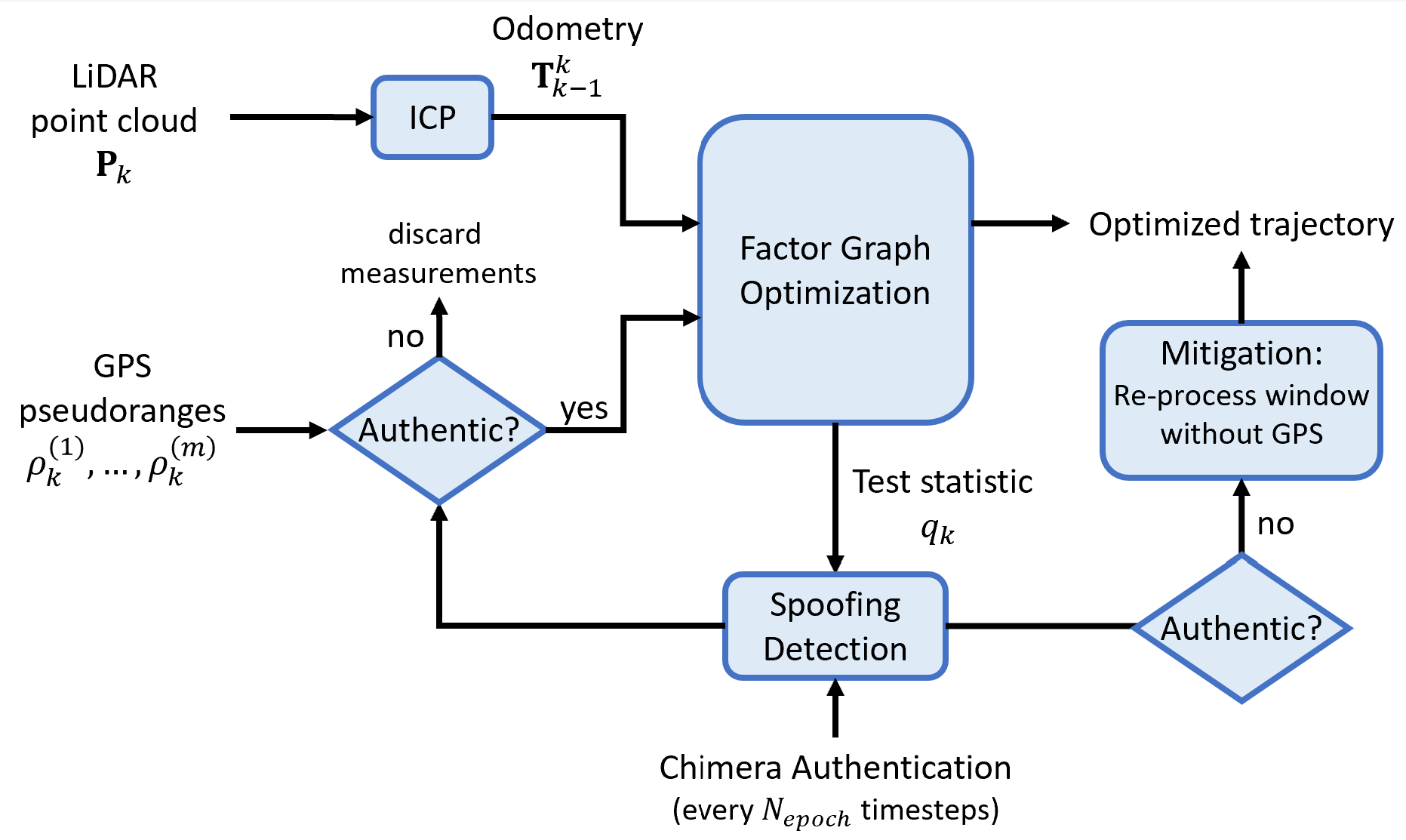
Figure 1: Block diagram illustrating our spoofing-resilient LiDAR-GPS factor graph framework. We operate over a window of measurements, for which LiDAR point clouds are registered with ICP to produce odometry measurements and combined with GPS pseudorange measurements in the factor graph. The vehicle trajectory over the window is estimated via factor graph optimization, and a chi-squared test statistic is computed from GPS residuals. If the statistic exceeds a threshold, an attack is detected, and it is mitigated by re-processing the window without GPS, and future GPS measurements are discarded from the factor graph. Chimera authentication overrides the detector as spoofing decision truth when available.

IV-A LiDAR-GPS Factor Graph

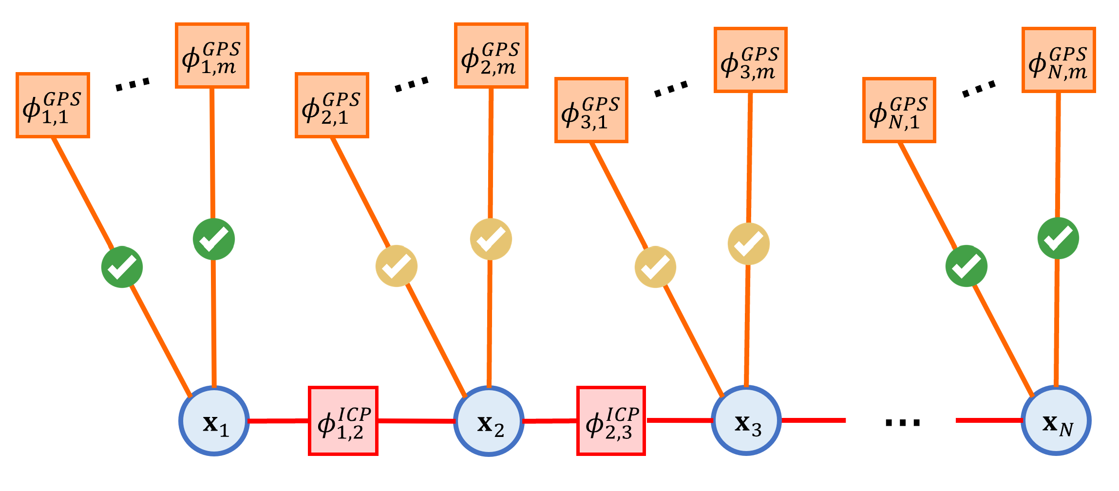
Figure 2: LiDAR-GPS factor graph structure over the Chimera epoch. Consecutive nodes are linked by LiDAR odometry factors $\phi^{\mathrm{\textnormal{ICP}}}_{i,i+1}$, while GPS range factors $\phi^{\mathrm{\textnormal{GPS}}}_{i,j}$ (where $j$ is satellite index) independently connect to nodes. The check symbols indicate that GPS has been deemed authentic, either by our detector (yellow) or by Chimera authentication (green)—in the unauthentic case GPS is excluded from the factor graph.

Our approach revolves around maintaining a tightly-coupled factor graph which integrates LiDAR and GPS for both localization and spoofing detection and mitigation, the structure of which is shown in Fig. 2. The nodes of our factor graph are vehicle poses $\mathbf{x}_{i}\in\mathbf{SE}(3)$ as described in Section III-D. The measurement models (Equations 7 and 11) and residuals (Equations 8 and 12) for GPS pseudoranges and LiDAR odometry factors are detailed in the following subsections.

IV-A1 GPS Pseudorange Factors

Given pose $\mathbf{x}_{i}$ with position component ${\mathbf{t}}_{i}$ and satellite $j$ at position $\mathbf{s}_{i}^{(j)}$ at time $i$, the expected GPS pseudorange measurement from satellite $j$ to node $i$ is

$$\hat{\rho}_{i}^{(j)}(\mathbf{x}_{i})=\left\|{\mathbf{t}}_{i}-\mathbf{s}_{i}^{(j)}\right\|_{2}.$$ (7)

Now, given received pseudorange measurement $\rho_{i}^{(j)}$, the GPS residual function can be defined as

$$\mathbf{e}_{i,j}^{\mathrm{\textnormal{GPS}}}(\mathbf{x}_{i})=\rho_{i}^{(j)}-\hat{\rho}_{i}^{(j)}(\mathbf{x}_{i}).$$ (8)

As the residual is a scalar in this case, the information matrix is also a scalar, $(\sigma^{\mathrm{\textnormal{GPS}}})^{-2}$, where $\sigma^{\mathrm{\textnormal{GPS}}}$ is the standard deviation of authentic GPS pseudoranges from Section III-C. In this work, we do not consider the effect of clock bias states in our pseudorange factors and simulated pseudorange measurements, but we will incorporate this into our measurement model in our future works.

IV-A2 LiDAR Odometry Factors

For LiDAR, we first use point-to-plane ICP (Iterative Closest Point) [20] to register successive point clouds and produce an odometry measurement. Given point clouds ${\mathbf{P}}_{i}$ and ${\mathbf{P}}_{i+1}$ at times $i$ and $i+1$, ICP produces an odometry measurement ${\mathbf{T}}_{i}^{i+1}$:

$${\mathbf{T}}_{i}^{i+1}\coloneqq\mathrm{\textnormal{icp}}({\mathbf{P}}_{i},{\mathbf{P}}_{i+1}).$$ (9)

${\mathbf{T}}_{i}^{i+1}$ is a rigid body transformation in $\mathbf{SE}(3)$, and can be written as

$${\mathbf{T}}_{i}^{i+1}=\begin{bmatrix}{\mathbf{R}}_{i}^{i+1}&{\mathbf{t}}_{i}^{i+1}\\ \mathbf{0}&1\end{bmatrix}\in\mathbb{R}^{4\times 4},$$ (10)

where ${\mathbf{R}}_{i}^{i+1}\in\mathbb{R}^{3\times 3}$ is the relative rotation between poses at times $i$ and $i+1$ and ${\mathbf{t}}_{i}^{i+1}\in\mathbb{R}^{3}$ is the relative translation between poses at times $i$ and $i+1$. The LiDAR odometry measurement model is the expected transformation between poses $i$ and $i+1$:

$$\hat{{\mathbf{T}}}_{i,i+1}(\mathbf{x}_{i},\mathbf{x}_{i+1})=\mathbf{x}_{i+1}(\mathbf{x}_{i})^{-1}.$$ (11)

The LiDAR odometry residual function is then defined as

$$\mathbf{e}_{i,i+1}^{\mathrm{\textnormal{ICP}}}(\mathbf{x}_{i},\mathbf{x}_{i+1})={\mathbf{T}}_{i}^{i+1}\ominus\hat{{\mathbf{T}}}_{i,i+1},$$ (12)

where $\ominus$ is the “ominus” operator defined in Section III-D. Intuitively, this residual is the difference between the expected and measured odometry transformation in $\mathfrak{se}(3)$ tangent space coordinates. Thus, $\mathbf{e}_{i,i+1}^{\mathrm{\textnormal{ICP}}}(\mathbf{x}_{i},\mathbf{x}_{i+1})\in\mathbb{R}^{6}$, and the information matrix for LiDAR odometry measurements is denoted by $\Omega^{\mathrm{\textnormal{ICP}}}\in\mathbb{R}^{6\times 6}$.

IV-A3 Optimization

We optimize the graph in a sliding window fashion. The window size is denoted by $N$, and as new nodes and measurements are added to the graph, previous nodes and edges are removed in order to maintain the maximum number of nodes in the graph as $N$. The objective for our factor graph over a single window can thus be written as

$${\mathbf{F}}(\mathbf{x})=\sum_{i=1}^{N}\sum_{j=1}^{m}(\mathbf{e}_{i,j}^{\mathrm{\textnormal{GPS}}})^{\mathsf{T}}(\sigma^{\mathrm{\textnormal{GPS}}})^{-2}\mathbf{e}_{i,j}^{\mathrm{\textnormal{GPS}}}$$ (13)

$$+\sum_{i=1}^{N-1}(\mathbf{e}_{i,i+1}^{\mathrm{\textnormal{ICP}}})^{\mathsf{T}}\Omega^{\mathrm{\textnormal{ICP}}}\mathbf{e}_{i,i+1}^{\mathrm{\textnormal{ICP}}}$$ (14)

The optimization carried out as described in Section III-E.

IV-B Spoofing Detection and Mitigation

To perform detection between Chimera authentication times, we design a chi-squared spoofing detector within our factor graph framework. Our detector computes a test statistic $q_{k}$ at time $k$ based on the information-normalized residuals of the GPS factors over the current window:

$$q_{k}=\sum_{i=i}^{N}\sum_{j=1}^{m}(\mathbf{e}_{i,j}^{\mathrm{\textnormal{GPS}}})^{\mathsf{T}}(\sigma^{\mathrm{\textnormal{GPS}}})^{-2}\mathbf{e}_{i,j}^{\mathrm{\textnormal{GPS}}}$$ (15)

Note that we do not include a normalization term based on the state estimate uncertainty (as typically done in the chi-squared detector with Kalman filter) as the factor graph does not maintain an estimate of state uncertainty. We then compare $q_{k}$ with a threshold $\tau$, which is pre-computed based on user-specified false alarm requirements. If $q_{k}>\tau$, then it is determined that spoofing is present in the measurements, otherwise the measurements are deemed authentic.

We now derive the computation of the threshold $\tau$. When the received GPS measurements are authentic and follow the nominal distribution with zero-mean Gaussian noise as shown in Equation (1), the GPS residuals $\mathbf{e}_{i,j}^{\mathrm{\textnormal{GPS}}}$ are distributed according to $\mathcal{N}(0,\sigma^{\mathrm{\textnormal{GPS}}})$ (assuming the estimated positions from FGO are close to ground-truth). Then, since the test statistic $q_{k}$ is computed from squaring the residuals (of which there are $Nm$) and normalizing by $(\sigma^{\mathrm{\textnormal{GPS}}})^{-2}$, $q_{k}$ follows a central chi-squared distribution with $n=Nm$ degrees of freedom. Thus, given a desired false alarm rate $\alpha$ to remain under, i.e., $\mathbb{P}(\mathrm{\textnormal{detection}}\,|\,\mathrm{\textnormal{not spoofed}})\leq\alpha$, we desire $\mathbb{P}(q_{k}\leq\tau)=1-\alpha$ for nominal conditions. Therefore, we compute $\tau$ as

$$\tau=\Phi^{-1}(1-\alpha;\ n=Nm)$$ (16)

where $\Phi^{-1}$ is the inverse cumulative distribution function (CDF) of the chi-squared distribution with $n=Nm$ degrees of freedom.

If spoofing is detected at time $k$, i.e., $q_{k}>\tau$, then any future GPS measurements are deemed unauthentic and the FGO henceforth proceeds with LiDAR only. Additionally, the current window is also re-processed with LiDAR measurements only, and GPS measurements discarded.

IV-C Chimera Authentication

After $N_{\mathrm{\textnormal{epoch}}}$ timesteps have passed, we receive Chimera authentication, which indicates whether the GPS measurements in the past Chimera epoch are authentic or unauthentic. If the Chimera authentication determines the GPS measurements to be authentic, we leverage this information and rely on the received measurements within our factor graph for $N$ measurements, which corresponds to the window size of our factor graph. However, if authentication fails, then we perform the same mitigation steps outlined in Section IV-B, where we discard GPS measurements and rely only on the LiDAR sensor. At this point, the spoofed victim could discontinue nominal operations and proceed according a fail-safe protocol, such as safely pulling over to the side of road, the specifics of which are outside the scope of this work.

V Experiments

We now describe details of our experimental validation, including the dataset used, spoofing attacks considered, baselines which we compare to, and parameters choices for our implementation.

V-A KITTI Dataset

We evaluate our approach using LiDAR data from the KITTI dataset [10] and simulated GPS pseudorange measurements based on the ground-truth positions and satellite ephemeris. In order to test our algorithm’s ability to detect and mitigate spoofing attacks over a 3-minute slow-channel Chimera epoch, we select all sequences from the raw data recordings of duration 3 minutes or longer. Table I lists the four sequences used in our experiments, their total duration in seconds, and the abbreviations used to refer to each one throughout the remainder of the paper.

TABLE I: KITTI Sequences

Sequence name	Abbreviation	Total duration
2011_09_30_drive_0018	0018	276 $\mathrm{s}$
2011_10_03_drive_0027	0027	455 $\mathrm{s}$
2011_09_30_drive_0028	0028	518 $\mathrm{s}$
2011_10_03_drive_0034	0034	466 $\mathrm{s}$

For all sequences, we consider a 200 second segment of the trajectory, which contains a full 180 second Chimera slow channel epoch. We simulate the Chimera authentication as occurring successfully at the first time step of the trajectory. As a result, the second Chimera authentication time occurs 180 seconds into the trajectory, and we simulate this as a failed authentication for each of the simulated GPS spoofing test scenarios described in Section V-B.

For all tested trajectories, we use the synced and rectified data in order to handle LiDAR motion distortion effects. To simulate GPS pseudorange measurements, we compute GPS satellite positions over time $\mathbf{s}_{i}^{(j)}$ using ephemeris data pulled from the location and timestamps of each sequence and follow the measurement model outlined in Section III-C. For ground-truth reference trajectories, we use the OXTS ground-truth positions and orientations provided by KITTI.

V-B Spoofing Attacks

We simulate spoofing attacks on the vehicle by generating a spoofed reference trajectory with added biases, then computing spoofed GPS pseudoranges based on the spoofed reference trajectory. Specifically, we consider a ramping attack that begins between the Chimera authentications, in which the spoofer introduces a bias which starts small and steadily ramps up to a large error. This type of attack is typically the most difficult to detect, as the spoofer can gradually induce error without any sudden jumps to alert a standard RAIM solution. And although the bias may start small, a spoofing victim under this attack can still experience significant positioning error over a sufficient time window, such as the 3 minute slow channel Chimera epoch.

For our experiments, we use a ramping bias which starts at 0 $\mathrm{m}$, and begins linearly increasing at rate $r_{\mathrm{\textnormal{spoof}}}$ $\mathrm{m}\mathrm{/}\mathrm{s}$ from time $T_{\mathrm{\textnormal{spoof}}}$ onward. We add the spoofing bias to the ENU positive $x$ (East) direction, and choose $T_{\mathrm{\textnormal{spoof}}}=100$ $\mathrm{s}$ for a total spoofing duration of 100 seconds. We run experiments for ramp rates of $r_{\mathrm{\textnormal{spoof}}}=$ 0.5 $\mathrm{m}\mathrm{/}\mathrm{s}$, 1.0 $\mathrm{m}\mathrm{/}\mathrm{s}$, and 2.0 $\mathrm{m}\mathrm{/}\mathrm{s}$, for maximum bias of 50 $\mathrm{m}$, 100 $\mathrm{m}$, and 200 $\mathrm{m}$ respectively. Fig. 3 shows the reference trajectories for each sequence, and spoofed trajectories for the chosen ramp rates.

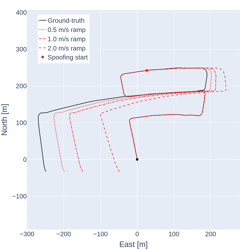
(a) 0018 reference trajectory with spoofed trajectories.

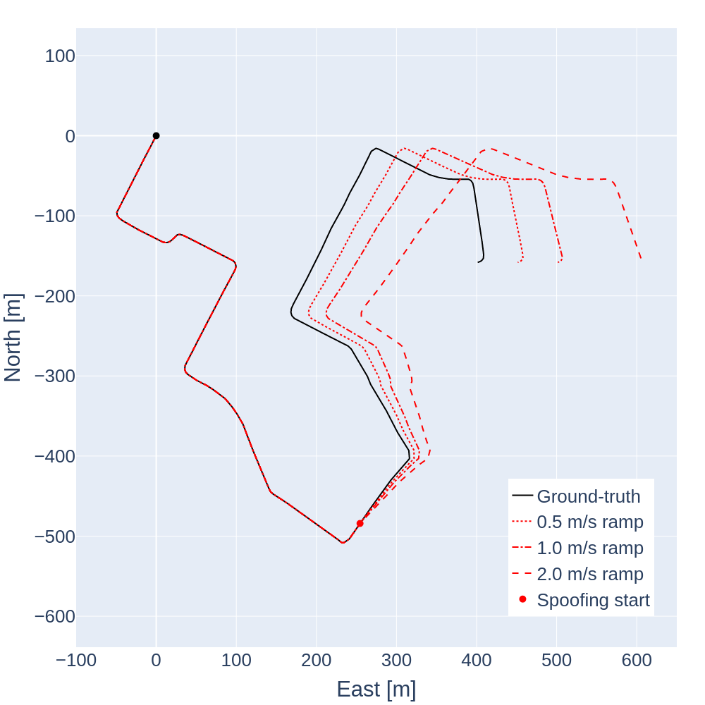
(b) 0027 reference trajectory with spoofed trajectories.

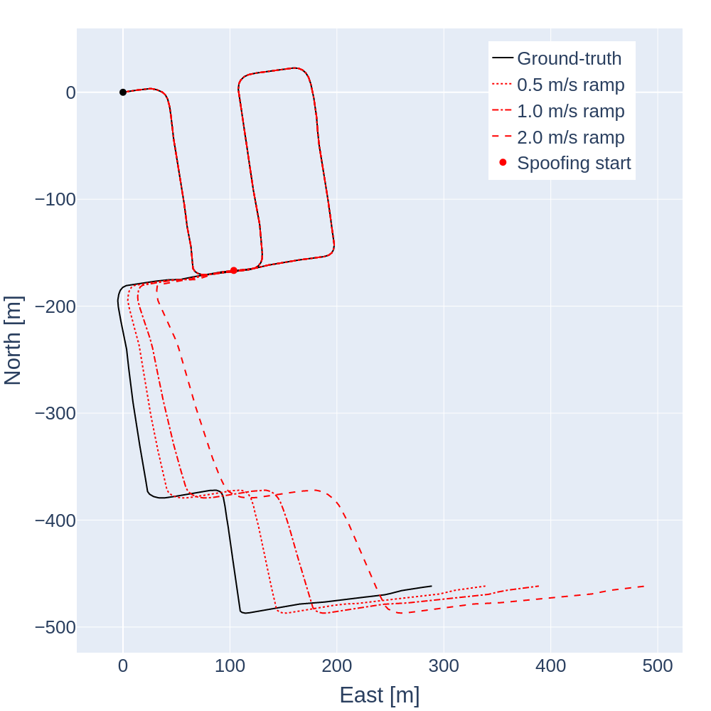
(c) 0028 reference trajectory with spoofed trajectories.

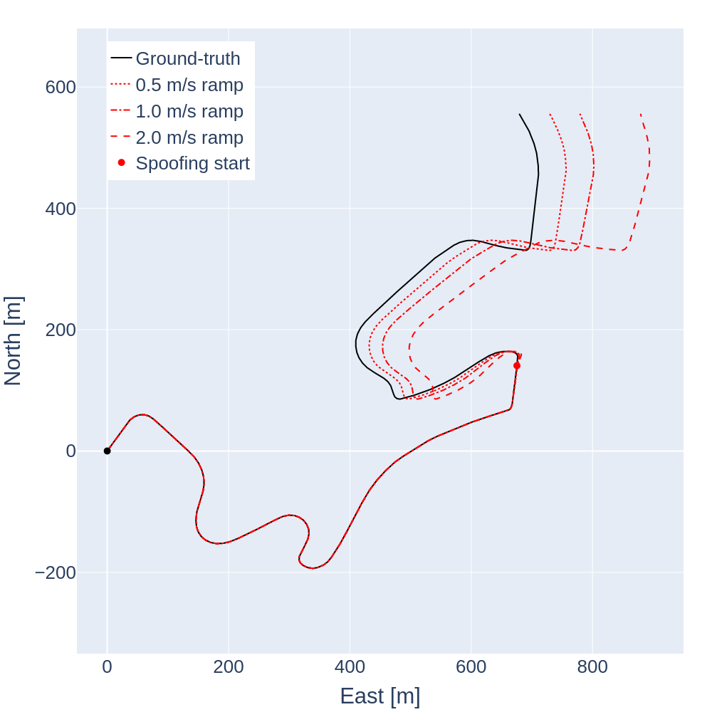
(d) 0034 reference trajectory with spoofed trajectories.

Figure 3: KITTI ground-truth reference trajectories shown with spoofed reference trajectories. The spoofing attacks begin at 100 seconds, introducing ramping error in the ENU positive $x$ (East) direction. Attacks for three different ramping rates are shown in different styles of red dashed lines.

V-C Metrics and Baselines for Comparison

In our experiments we compare our approach with two baseline approaches. The first baseline is “Odometry only,” in which only LiDAR odometry is used to localize the vehicle between Chimera authentications, and GPS measurements are only used at the slow channel 3 minute interval. The second baseline is “Naive FGO,” in which LiDAR-GPS factor graph optimization produces a fused state estimate but no spoofing detection or mitigation is employed. Finally, “SR FGO” refers to our spoofing-resilient LiDAR-GPS factor graph optimization approach presented in Section IV.

For characterizing performance, we consider $L^{2}$ norm position error, which is calculated as $e_{k}=\left\|{\mathbf{t}}_{k}^{\mathrm{\textnormal{ref}}}-{\mathbf{t}}_{k}^{\mathrm{\textnormal{est}}}\right\|_{2}$ for each time index $k$ of the trajectory, where ${\mathbf{t}}_{k}^{\mathrm{\textnormal{ref}}}$ is the reference trajectory position at time $k$ and ${\mathbf{t}}_{k}^{\mathrm{\textnormal{est}}}$ is the estimated trajectory position at time $k$. In addition, we consider two metrics: mean $L^{2}$ norm position error and maximum $L^{2}$ norm position error, which are simply computed as $e_{\mathrm{\textnormal{mean}}}=\mathrm{\textnormal{mean}}_{k}(e_{k})$ and $e_{\mathrm{\textnormal{max}}}=\mathrm{\textnormal{max}}_{k}(e_{k})$ respectively, and hereafter referred to more concisely as mean error and max error.

V-D Parameters

We discretize time with $\Delta t=0.1$ $\mathrm{s}$, and use LiDAR point clouds from the KITTI sequences taken at 10 $\mathrm{H}\mathrm{z}$. We use $\Sigma^{\mathrm{\textnormal{ICP}}}=\mathrm{\textnormal{diag}}(0.01,0.01,0.01,0.05,0.05,0.05)$ as the standard deviation of LiDAR ICP odometry measurements, where the 0.01 values correspond to the rotational components of $\mathfrak{se}(3)$ (equivalent to 0.01 $\mathrm{r}\mathrm{a}\mathrm{d}$ std.) and the 0.05 values correspond to the translational components (0.05 $\mathrm{m}$ std.). We simulate GPS measurements at 1 $\mathrm{H}\mathrm{z}$ and take $\sigma^{\mathrm{\textnormal{GPS}}}=7.0$ $\mathrm{m}$ according to the typical User-equivalent Range Error (UERE) for a single-frequency receiver [21]. We choose a window size of $N=100$, and shift the window by 10 steps per iteration. $\alpha=0.001$ is chosen as the false alarm rate for our detector.

For point-to-plane ICP LiDAR registration, we use the Open3D [22] function registration_icp with parameter TransformationEstimationPointToPlane() class and threshold value of 1.0. We use SymForce [23], a recently developed state-of-the-art symbolic computation library for robotics applications, as the factor graph optimization backend for our method. Our code is available online at our GitHub repository.

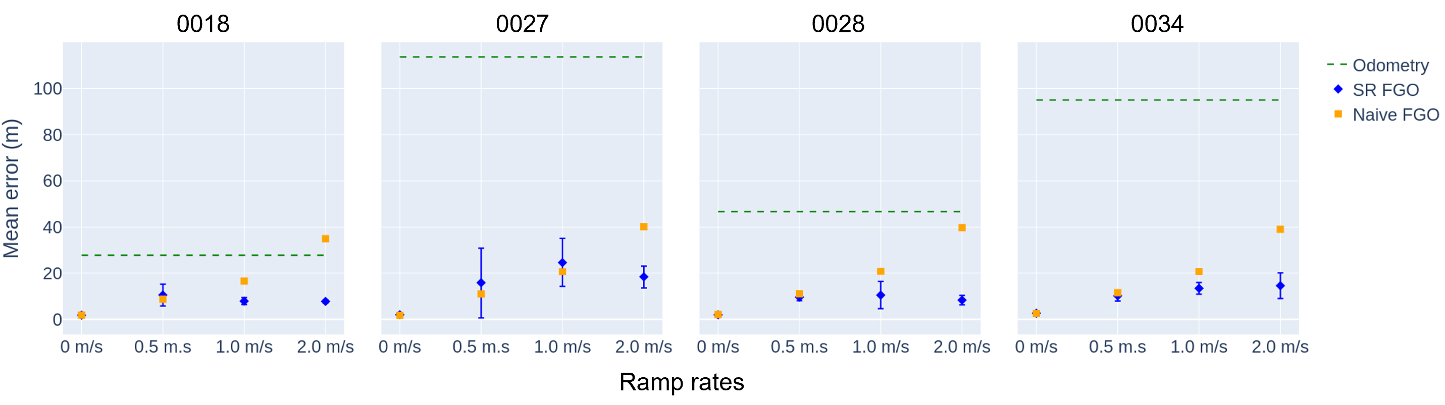
(a) Mean $L^{2}$ norm position error compared across increasing ramp rates.

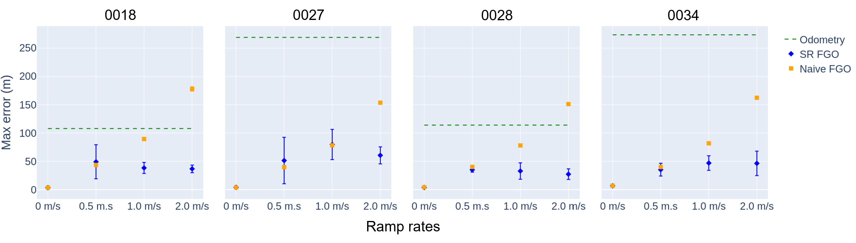
(b) Max $L^{2}$ norm position error compared across increasing ramp rates.

Figure 4: Comparison of our approach with baselines in mean and maximum trajectory error for different sequences and spoofing ramp rates. Each subplot shows the mean/maximum trajectory error values of LiDAR odometry (green), Naive FGO (red), and SR FGO (blue) across increasing spoofing attack rates for a specific sequence. LiDAR odometry is unaffected by spoofing, and is thus shown as horizontal lines, while results for Naive FGO and SR FGO are each averaged over 10 Monte Carlo runs, with error bars indicating one standard deviation. Compared to the Naive FGO, SR FGO mitigates errors as spoofing ramp rate increases.

VI Results

Now we present the experimental validation results of our spoofing-resilient factor graph algorithm. We run our algorithm along with the two baselines (Section V-C) on four KITTI sequences (Table I), for both nominal GPS measurements and various ramping GPS spoofing attacks (shown in Fig. 3). We compare performance in terms of $L^{2}$ norm error over time, as well as mean and max $L^{2}$ norm error, and also include case studies on window size variation and detection statistics.

VI-A Comprehensive Comparison

We begin by presenting a comprehensive comparison of our approach against the two baselines considered, across the different KITTI sequences and multiple spoofing ramp rates. These results are illustrated in Fig. 4. We see that for all sequences, the mean and max $L^{2}$ norm error of our SR FGO approach remains under that of LiDAR odometry only. In particular, as the spoofing attack rate increases, the Naive FGO mean and max errors increase, and in some cases eventually exceed the levels of odometry drift, whereas the SR FGO errors are successfully mitigated in all cases and remain bounded under odometry.

VI-B Comparison of Errors over Time under Spoofed Conditions

Next, we focus on the spoofed case of $r_{\mathrm{\textnormal{spoof}}}=2.0$ $\mathrm{m}\mathrm{/}\mathrm{s}$, and compare the $L^{2}$ position error over time of our SR FGO approach against the two baselines Odometry only and Naive FGO. Fig. 5 shows a comparison plot for each KITTI trajectory. In each plot, 20 Monte Carlo runs of Naive and SR FGO are shown, and the start of the spoofing attack at 100 seconds is indicated by the vertical red dashed line. For each trajectory, we see that LiDAR odometry suffers from significant drift over time, on the order of 100s to 200s of meters of final $L^{2}$ norm position error after 200 seconds. For both Naive FGO and SR FGO, $L^{2}$ position errors remain under 5.0 $\mathrm{m}$ for the first 100 seconds during authentic conditions. However, after the start of the attack at 100 seconds, the Naive FGO approach is heavily influenced by the spoofing attack, and its $L^{2}$ norm position error diverges, with final error exceeding that of LiDAR odometry in sequences 0018 and 0028. On the other hand, our SR FGO approach is able to consistently detect and mitigate the spoofing attack, and keep position errors bounded to under odometry drift levels.

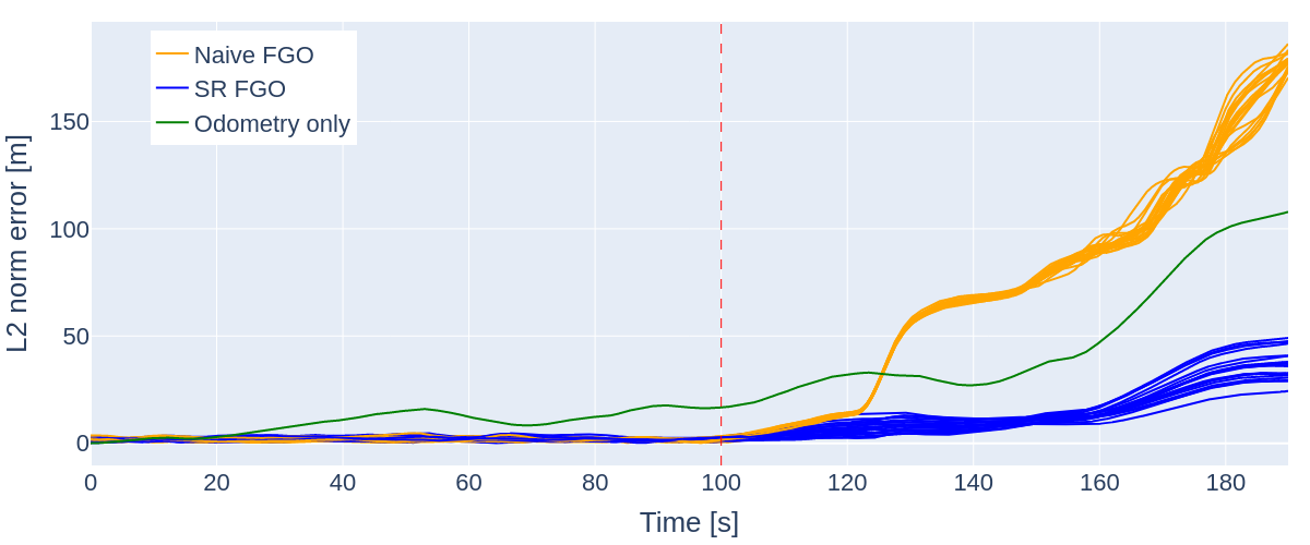
(a) Sequence 0018

(b) Sequence 0027

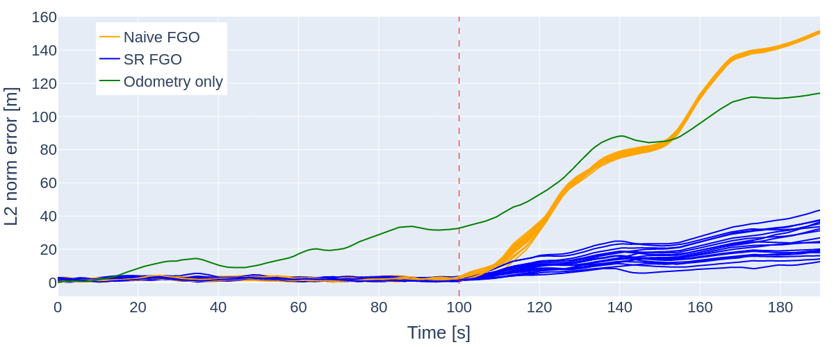
(c) Sequence 0028

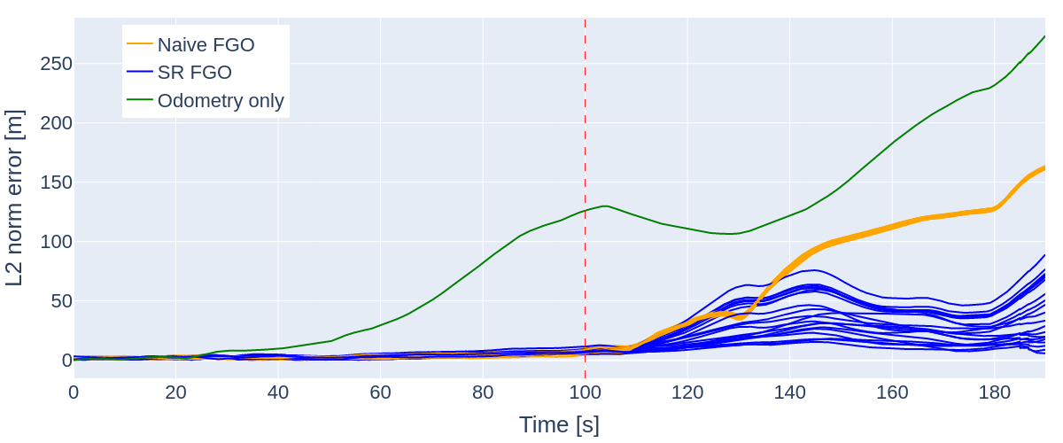
(d) Sequence 0034

Figure 5: Comparison of trajectory errors for three different approaches on KITTI sequences. For each plot, LiDAR odometry error over time is shown in green, while 20 Monte Carlo runs each of Naive FGO and SR FGO are shown in red and blue respectively. In each sequence, our spoofing-resilient FGO mitigates the spoofing attack, bounding errors during the Chimera epoch to well under odometry drift levels.

VI-C Window Size Comparison

Now, we perform a case study to analyze to effect of varying window size on the performance of our algorithm. Table II(d) shows a comparison of mean and max $L^{2}$ norm position error as well as average iteration time across a range of increasing window sizes for each sequence.

TABLE II: Window Size Comparison under 0.2 $\mathrm{m}\mathrm{/}\mathrm{s}$ Spoofing averaged over 20 Monte Carlo runs. Performance initially improves with increasing window size then saturates between 5 $\mathrm{s}$ to 20 $\mathrm{s}$, while average iteration time increases consistently with window size as expected. Window size is expressed in timesteps (of length 0.1 $\mathrm{s}$).

Window size	Mean error	Max error	Avg. iteration time
20	26.1 $\mathrm{m}$	101.0 $\mathrm{m}$	0.144 $\mathrm{s}$
50	8.66 $\mathrm{m}$	41.1 $\mathrm{m}$	0.469 $\mathrm{s}$
100	9.75 $\mathrm{m}$	46.2 $\mathrm{m}$	1.25 $\mathrm{s}$
200	11.5 $\mathrm{m}$	59.5 $\mathrm{m}$	3.57 $\mathrm{s}$
300	13.9 $\mathrm{m}$	63.6 $\mathrm{m}$	6.69 $\mathrm{s}$

(a) Sequence 0018

Window size	Mean error	Max error	Avg. iteration time
20	189.4 $\mathrm{m}$	372.3 $\mathrm{m}$	0.130 $\mathrm{s}$
50	28.1 $\mathrm{m}$	78.4 $\mathrm{m}$	0.445 $\mathrm{s}$
100	20.9 $\mathrm{m}$	63.9 $\mathrm{m}$	1.13 $\mathrm{s}$
200	29.6 $\mathrm{m}$	92.3 $\mathrm{m}$	3.37 $\mathrm{s}$
300	30.7 $\mathrm{m}$	94.8 $\mathrm{m}$	5.78 $\mathrm{s}$

(b) Sequence 0027

Window size	Mean error	Max error	Avg. iteration time
20	47.6 $\mathrm{m}$	112.6 $\mathrm{m}$	0.139 $\mathrm{s}$
50	15.2 $\mathrm{m}$	44.3 $\mathrm{m}$	0.456 $\mathrm{s}$
100	12.5 $\mathrm{m}$	34.0 $\mathrm{m}$	1.21 $\mathrm{s}$
200	7.07 $\mathrm{m}$	24.1 $\mathrm{m}$	3.41 $\mathrm{s}$
300	15.9 $\mathrm{m}$	42.8 $\mathrm{m}$	6.47 $\mathrm{s}$

(c) Sequence 0028

Window size	Mean error	Max error	Avg. iteration time
20	83.8 $\mathrm{m}$	241.5 $\mathrm{m}$	0.144 $\mathrm{s}$
50	25.8 $\mathrm{m}$	110.4 $\mathrm{m}$	0.469 $\mathrm{s}$
100	23.8 $\mathrm{m}$	106.4 $\mathrm{m}$	2.64 $\mathrm{s}$
200	28.8 $\mathrm{m}$	127.3 $\mathrm{m}$	3.38 $\mathrm{s}$
300	25.5 $\mathrm{m}$	121.1 $\mathrm{m}$	6.43 $\mathrm{s}$

(d) Sequence 0034

As expected, for all sequences, the average iteration time increases with window size, as the factor graph optimization must be done over a larger window with more measurements. We also observe high rate of false detection for the smallest window size of 20. This is to be expected, as the test statistic will be more sensitive to measurement noise and small errors in the trajectory estimates for a smaller window, and thus this window size behaves similarly to LiDAR odometry only in performance.

For all sequences, we also notice that improvement in mean and max error saturates as we increase the window size, occurring at $N=50$ for sequence 0018, $N=100$ for sequence 0027, $N=200$ for sequence 0028, and $N=100$ for sequence 0034. This is most likely due to that fact that, as window size increases, a larger window of the trajectory is re-processed when spoofing is detected. If spoofing is detected for a window with majority authentic measurements but some spoofed measurements towards the end, then we may discard more authentic measurements which may adversely affect the overall positioning performance. The results of this case study validate our general choice of window size $N=100$ for our experiments.

VI-D Detection Statistics

Finally, we examine the detection statistics for our algorithm, first running 100 Monte Carlo simulations for the nominal, unspoofed case to test the false alarm rate of our detector. These runs are plotted along with the corresponding detection threshold in Fig. 6(a). The parameter $\alpha=0.001$ corresponds to the false alarm probability of a single trial, so across a 180 second long Chimera epoch with 180 trials (one for every GPS measurement at 1 Hz), the probability of a false alarm occurring during the Chimera epoch is $1-(1-\alpha)^{180}=0.165$. Across the 100 Monte Carlo runs, there were a total of 9 false alarms, for an empirical per run false alarm rate of 0.09, and 15 total individual trial false alarms out of 18000 individual trials for an empirical per trial false alarm rate of 0.000833. Thus, we see that our detector satisfies the desired false alarm rate requirements set by the user.

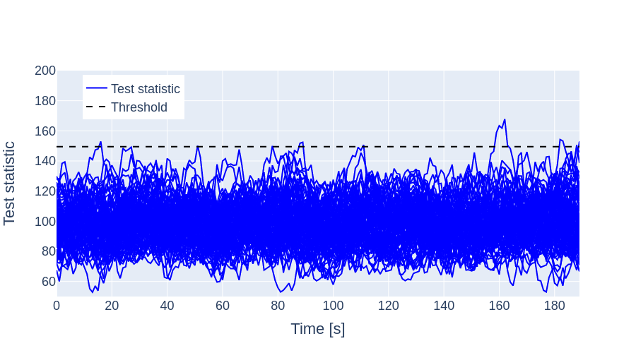
(a) Spoofing test statistic plotted for 100 Monte Carlo runs under nominal (authentic) conditions. Our detector satisfies the prescribed false alarm rate of $\alpha=0.001$.

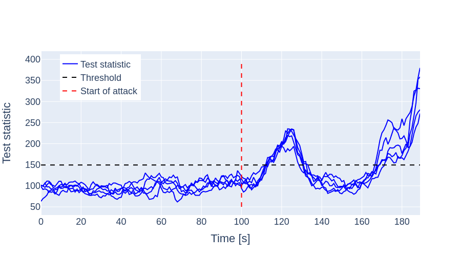
(b) Spoofing test statistic plotted for 10 Monte Carlo runs under a spoofing attack of $r_{\mathrm{\textnormal{spoof}}}=1.0$ $\mathrm{m}\mathrm{/}\mathrm{s}$. The statistic crosses the threshold shortly after the attack for all 10 of the runs.

Figure 6: Monte Carlo simulations of spoofing test statistic plotted over time for both nominal and spoofed conditions. Our detection method remains under the user specified false alarm rates, while consistently detecting the presence of a sufficiently large spoofing attack.

We also perform Monte Carlo simulation for the spoofed case for an attack with $r_{\mathrm{\textnormal{spoof}}}=1.0$ $\mathrm{m}\mathrm{/}\mathrm{s}$, shown in Fig. 6(b). In each of the 10 runs, the test statistic crosses the threshold shortly after the start of the attack, successfully detecting it, with a average time to detect of 11.2 seconds.

VII Conclusion

In this work, we present a new framework for spoofing-resilient LiDAR-GPS factor graph fusion for Chimera GPS, which provides continuous and secure state estimation between Chimera authentication times. Our approach fuses LiDAR and GPS measurements with factor graph optimization, and computes a test statistic for spoofing detection based on the GPS factor residuals. From this test statistic, our approach determines when to leverage the unauthenticated GPS measurements during the Chimera epoch, in order to improve localization performance when GPS is likely authentic. We evaluate our approach with real-world data from the KITTI self-driving dataset, using sequences which span the Chimera slow channel 3-minute epoch. Our results demonstrate rapid detection and effective mitigation of spoofing attacks during vulnerable periods between authentications.

This work contributes towards the problem of designing LiDAR-GPS factor graph localization that is robust to GPS spoofing attacks. Our approach is designed around the Chimera signal enhancement, which will be a critical utility to authenticating GPS measurements against spoofing. Between Chimera authentications, we utilize the LiDAR sensor measurements to validate and strategically leverage GPS measurements to improve localization performance during authentic conditions, while maintaining resilience against experienced attacks during spoofing. Our work addresses the research gap for LiDAR-GPS fusion platforms, and takes an important step towards ensuring continuous navigation security for users of the future Chimera-enhanced GPS.

References

- [1] G. Wan, X. Yang, R. Cai, H. Li, Y. Zhou, H. Wang, and S. Song, “Robust and precise vehicle localization based on multi-sensor fusion in diverse city scenes,” in 2018 IEEE international conference on robotics and automation (ICRA). IEEE, 2018, pp. 4670–4677.
- [2] J. Shen, J. Y. Won, Z. Chen, and Q. A. Chen, “Drift with Devil: Security of Multi-Sensor Fusion based Localization in High-Level Autonomous Driving under GPS Spoofing,” in 29th USENIX Security Symposium (USENIX Security 20), 2020, pp. 931–948.
- [3] J. M. Anderson, K. L. Carroll, N. P. DeVilbiss, J. T. Gillis, J. C. Hinks, B. W. O’Hanlon, J. J. Rushanan, L. Scott, and R. A. Yazdi, “Chips-message robust authentication (chimera) for GPS civilian signals,” in Proceedings of the 30th International Technical Meeting of The Satellite Division of the Institute of Navigation (ION GNSS+ 2017), 2017, pp. 2388–2416.
- [4] T. Mina, A. Kanhere, A. Shetty, and G. Gao, “GPS Spoofing-Resilient Filtering with Chimera and Self-Contained Odometry,” in Proceedings of the 35th International Technical Meeting of the Satellite Division of The Institute of Navigation (ION GNSS+ 2022), 2022, pp. 3768–3782.
- [5] A. V. Kanhere, T. Mina, A. Shetty, and G. Gao, “Factor Graph-based Spoofing Mitigation using the Chimera Signal Enhancement,” in Proceedings of the 35th International Technical Meeting of the Satellite Division of The Institute of Navigation (ION GNSS+ 2022), 2022, pp. 958–968.
- [6] X. Li, H. Wang, S. Li, S. Feng, X. Wang, and J. Liao, “GIL: a tightly coupled GNSS PPP/INS/LiDAR method for precise vehicle navigation,” Satellite Navigation, vol. 2, no. 1, pp. 1–17, 2021.
- [7] W. Wen, T. Pfeifer, X. Bai, and L.-T. Hsu, “Factor graph optimization for GNSS/INS integration: A comparison with the extended Kalman filter,” NAVIGATION: Journal of the Institute of Navigation, vol. 68, no. 2, pp. 315–331, 2021.
- [8] D. Chen and G. X. Gao, “Probabilistic graphical fusion of LiDAR, GPS, and 3D building maps for urban UAV navigation,” Navigation, vol. 66, no. 1, pp. 151–168, 2019.
- [9] X. He, S. Pan, W. Gao, and X. Lu, “LiDAR-Inertial-GNSS Fusion Positioning System in Urban Environment: Local Accurate Registration and Global Drift-Free,” Remote Sensing, vol. 14, no. 9, p. 2104, 2022.
- [10] A. Geiger, P. Lenz, C. Stiller, and R. Urtasun, “Vision meets robotics: The KITTI dataset,” The International Journal of Robotics Research, vol. 32, no. 11, pp. 1231–1237, 2013.
- [11] M. L. Psiaki and T. E. Humphreys, “GNSS spoofing and detection,” Proceedings of the IEEE, vol. 104, no. 6, pp. 1258–1270, 2016.
- [12] J. Hinks, J. T. Gillis, P. Loveridge, G. Myer, J. J. Rushanan, S. Stoyanov et al., “Signal and data authentication experiments on NTS-3,” in Proceedings of the 34th International Technical Meeting of the Satellite Division of The Institute of Navigation (ION GNSS+ 2021), 2021, pp. 3621–3641.
- [13] N. Sünderhauf and P. Protzel, “Switchable constraints for robust pose graph SLAM,” in 2012 IEEE/RSJ International Conference on Intelligent Robots and Systems. IEEE, 2012, pp. 1879–1884.
- [14] Ç. Tanıl, S. Khanafseh, M. Joerger, and B. Pervan, “An INS monitor to detect GNSS spoofers capable of tracking vehicle position,” IEEE Transactions on Aerospace and Electronic Systems, vol. 54, no. 1, pp. 131–143, 2017.
- [15] J. L. Blanco-Claraco, “A tutorial on SE(3) transformation parameterizations and on-manifold optimization,” arXiv preprint arXiv:2103.15980, 2021.
- [16] T. D. Barfoot, State estimation for robotics. Cambridge University Press, 2017.
- [17] J. Sola, J. Deray, and D. Atchuthan, “A micro lie theory for state estimation in robotics,” arXiv preprint arXiv:1812.01537, 2018.
- [18] F. Dellaert and M. Kaess, “Factor graphs for robot perception,” Foundations and Trends® in Robotics, vol. 6, no. 1-2, pp. 1–139, 2017.
- [19] G. Grisetti, R. Kümmerle, C. Stachniss, and W. Burgard, “A tutorial on graph-based SLAM,” IEEE Intelligent Transportation Systems Magazine, vol. 2, no. 4, pp. 31–43, 2010.
- [20] P. J. Besl and N. D. McKay, “Method for registration of 3-D shapes,” in Sensor fusion IV: control paradigms and data structures, vol. 1611. Spie, 1992, pp. 586–606.
- [21] E. D. Kaplan and C. Hegarty, Understanding GPS/GNSS: principles and applications. Artech house, 2017.
- [22] Q.-Y. Zhou, J. Park, and V. Koltun, “Open3D: A modern library for 3D data processing,” arXiv preprint arXiv:1801.09847, 2018.
- [23] H. Martiros, A. Miller, N. Bucki, B. Solliday, R. Kennedy, J. Zhu, T. Dang, D. Pattison, H. Zheng, T. Tomic, P. Henry, G. Cross, J. VanderMey, A. Sun, S. Wang, and K. Holtz, “SymForce: Symbolic Computation and Code Generation for Robotics,” in Proceedings of Robotics: Science and Systems, 2022.