New Type of Traversable Wormhole${}^{\,\S}$

Frans R. KlinkhamerNew Type of Traversable Wormhole

1

1

We review a new traversable-wormhole solution of the gravitational field equation of general relativity without exotic matter. Instead of having exotic matter to keep the wormhole throat open, the solution relies on a 3-dimensional “spacetime defect,” which is characterized by a locally vanishing metric determinant. We also discuss the corresponding multiple-vacuum-defect-wormhole solution and possible experimental signatures from a “gas” of vacuum-defect wormholes. Multiple vacuum-defect wormholes appear to allow for backward time travel.

general relativity, wormhole solution

1 Introduction

Here is an ultra-brief history of theoretical ideas on wormholes in five crucial dates:

• 1915, Einstein’s general relativity is established with spacetime acting as a dynamical quantity (a summary is published one year later [1]).

• 1935, the metric of the Einstein-Rosen “bridge” connecting different parts of spacetime is presented [2], but a traveller cannot go across, as a singularity will be encountered first.

• 1955, Wheeler [3] considers a multiply-connected 3-space and gives a sketch of a “tunnel” or “handle” in his Figure 7 (here, reproduced as Figure 1); in the following years, he also discusses a spacetime foam teeming with (Euclidean) wormholes of Planckian length scales, $l_{P}\equiv\sqrt{\hbar\,G/c^{3}}\sim 10^{-35}\,\text{m}$ (a later review paper appears in 1968 [4]).

• 1973, two papers [5, 6] are published with a metric suitable for a traversable wormhole.

• 1988, Morris and Thorne [7] show that certain wormhole solutions of the Einstein equation may be traversable, but at a high price: exotic matter.

In this contribution, we discuss a recently discovered wormhole solution [8, 9], where the price for traversability is paid not by the matter but by the spacetime structure. This new wormhole solution is based on earlier work [10], as will be explained later on.

For completeness, we should perhaps mention that the metric of the Einstein-Rosen bridge does not solve the vacuum gravitational field equation, as noted somewhat obliquely in the original paper [2]. See, e.g., Ref. [11] for further discussion.

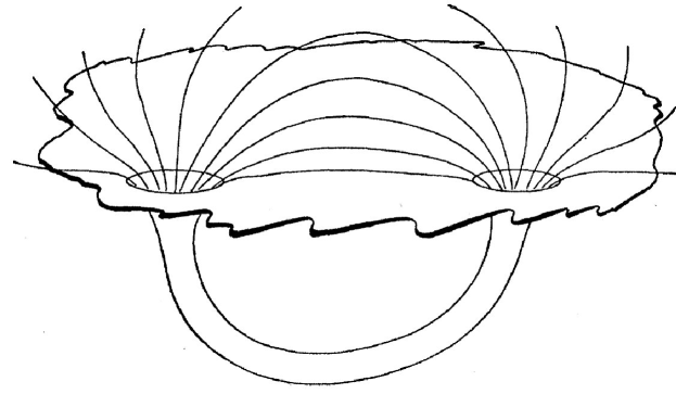
Figure 1: First sketch of a wormhole in the modern physics literature from Wheeler’s 1955 paper. [Image credit: J.A. Wheeler, “Geons,” Phys. Rev. 97, 511 (1955); DOI: https://doi.org/10.1103/PhysRev.48.73]

2 Exotic-Matter Wormhole

Morris and Thorne (MT) considered a simple metric in Box 2 of their 1988 paper [7]. Specifically, they discuss the following special case of a more general metric (setting $c=1$):

$$ds^{2}\,\Big{|}^{\text{(EBMT-special)}}\equiv g_{\mu\nu}(x)\,dx^{\mu}\,dx^{\nu}\,\Big{|}^{\text{(EBMT-special)}}$$ (1)

$$=-dt^{2}+dl^{2}+\left(b_{0}^{2}+l^{2}\right)\,\Big{[}d\theta^{2}+\sin^{2}\theta\,d\phi^{2}\Big{]}\,,$$

with a nonzero real constant $b_{0}$ (taken to be positive, for definiteness). The coordinates $t$ and $l$ in (1) range over $(-\infty,\,\infty)$, while the coordinates $\theta\in[0,\,\pi]$ and $\phi\in[0,\,2\pi)$ are the standard spherical polar coordinates [strictly speaking, we should use two coordinate patches for the 2-sphere, for example, by stereographic projections from the North Pole and the South Pole].

Earlier discussions of this type of metric have appeared in independent papers by Ellis [5] and Bronnikov [6]. Hence, we have added “EB” to the suffix of (1).

The resulting Ricci and Kretschmann curvature scalars are

$$R\,\Big{|}^{\text{(EBMT-special)}} = -2\;\frac{b_{0}^{2}}{\left(b_{0}^{2}+l^{2}\right)^{2}}\,,$$ (2a)

$$K\,\Big{|}^{\text{(EBMT-special)}} = 12\;\frac{\left(b_{0}^{2}\right)^{2}}{\left(b_{0}^{2}+l^{2}\right)^{4}}\,,$$ (2b)

both of which are seen to vanish as $l\to\pm\infty$. Indeed, two distinct flat Minkowski spacetimes are approached for $l\to\pm\infty$; see Figure 2.

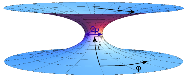
Figure 2: Embedding diagram of the wormhole spacetime with metric (1) for $t=\text{const}$ and $\theta=\pi/2$, with temporary definitions $2\rho\equiv 2b_{0}>0$ and $r\equiv\sqrt{b_{0}^{2}+l^{2}}\,$. [Image credit: O. James, E. von Tunzelmann, P. Franklin, and K.S. Thorne, “Visualizing Interstellar’s Wormhole,” arXiv:1502.03809; DOI: https://doi.org/10.48550/arXiv.1502.03809]

The EBMT wormhole is traversable, as shown by items (d) and (e) of Box 2 in Morris and Thorne’s paper [7] and by Figure 6 in Ellis’ paper [5]. Incidentally, the wormhole of Figure 2 is of the inter-universe type, connecting two distinct asymptotically-flat spaces, whereas the wormhole of Figure 1 is an intra-universe wormhole, connecting to a single asymptotically-flat space. Figure 1 also illustrates two further properties of a wormhole, namely, the wormhole “mouths” (essentially the boundaries between the wormhole tube and the near-flat surrounding space) and the wormhole “throat” (the wormhole tube proper between the wormhole mouths).

The crucial question, however, concerns the dynamics: can this EBMT wormhole metric be a solution of the Einstein equation? Morris and Thorne’s brilliant idea [7] was to use an engineering approach: fix the desired specifications and see what it takes.

With the metric (1) for a traversable wormhole, the Einstein equation,

$$R_{\mu\nu}-{\textstyle\frac{1}{2}}\,g_{\mu\nu}\,R=8\pi G\>T_{\mu\nu}\,,$$ (3)

requires these components of the energy-momentum tensor [7]:

$$T^{\,t}_{\;\;\,t}\,\Big{|}^{\text{(EBMT-special)}} = \frac{1}{8\pi G}\;\frac{b_{0}^{2}}{\left(b_{0}^{2}+l^{2}\right)^{2}}\,,$$ (4a)

$$T^{\,l}_{\;\;\,l}\,\Big{|}^{\text{(EBMT-special)}} = -\frac{1}{8\pi G}\;\frac{b_{0}^{2}}{\left(b_{0}^{2}+l^{2}\right)^{2}}\,,$$ (4b)

$$T^{\,\theta}_{\;\;\,\theta}\,\Big{|}^{\text{(EBMT-special)}} = \frac{1}{8\pi G}\;\frac{b_{0}^{2}}{\left(b_{0}^{2}+l^{2}\right)^{2}}\,,$$ (4c)

$$T^{\,\phi}_{\;\;\,\phi}\,\Big{|}^{\text{(EBMT-special)}} = \frac{1}{8\pi G}\;\frac{b_{0}^{2}}{\left(b_{0}^{2}+l^{2}\right)^{2}}\,,$$ (4d)

with all other components vanishing. As the energy density is given by $\rho=T^{\,tt}=-T^{\,t}_{\;\;\,t}$, we have $\rho<0$ from (4a), which certainly corresponds to nonstandard matter. Moreover, we obtain the following inequality for the radial null vector $\overline{k}^{\,\mu}=(1,\,1,\,0,\,0)$:

$$T^{\,\mu}_{\;\;\,\nu}\,\overline{k}_{\mu}\,\overline{k}^{\,\nu}\,\Big{|}^{\text{(EBMT-special)}}=\frac{1}{8\pi G}\;\frac{b_{0}^{2}}{\left(b_{0}^{2}+l^{2}\right)^{2}}\;\big{[}-1-1\big{]}<0\,,$$ (5)

which corresponds to a violation of the Null-Energy-Condition (NEC).

As stressed by Morris and Thorne [7], the problem is that it is not clear if the needed exotic matter really exists.

3 New Wormhole

3.1 Special Ansatz

We now propose a somewhat different metric [8]:

$$ds^{2}\,\Big{|}^{\text{(K-special)}}\equiv g_{\mu\nu}(x)\,dx^{\mu}\,dx^{\nu}\,\Big{|}^{\text{(K-special)}}$$

$$=-dt^{2}+\frac{\xi^{2}}{\xi^{2}+\lambda^{2}}\;d\xi^{2}+\left(b_{0}^{2}+\xi^{2}\right)\,\Big{[}d\theta^{2}+\sin^{2}\theta\,d\phi^{2}\Big{]}\,,$$ (6)

with nonzero real constants $\lambda$ and $b_{0}$ (both taken to be positive, for definiteness) and coordinates $t$ and $\xi$ ranging over $(-\infty,\,\infty)$. The resulting Ricci and Kretschmann curvature scalars are

$$R\,\Big{|}^{\text{(K-special)}} = -2\;\frac{b_{0}^{2}-\lambda^{2}}{\left(b_{0}^{2}+\xi^{2}\right)^{2}}\,,$$ (7a)

$$K\,\Big{|}^{\text{(K-special)}} = 12\;\frac{\left(b_{0}^{2}-\lambda^{2}\right)^{2}}{\left(b_{0}^{2}+\xi^{2}\right)^{4}}\,,$$ (7b)

both of which are finite, smooth, and vanishing as $\xi\to\pm\infty$.

The metric $g_{\mu\nu}(x)$ from (3.1) is degenerate with a vanishing determinant $g(x)\equiv\det[g_{\mu\nu}(x)]$ at $\xi=0$. In physical terms, this 3-dimensional hypersurface at $\xi=0$ corresponds to a “spacetime defect.” The terminology is by analogy with crystallographic defects in an atomic crystal (these crystallographic defects are typically formed during a rapid crystallization process).

The new wormhole metric (3.1) did not fall out of the sky but is a direct follow-up of earlier work on a particular “time defect” that regularizes the big bang [10]. That particular paper [10] contains further references to previous work on this type of “spacetime defect.”

We now use Morris and Thorne’s engineering approach. The Einstein equation (3) for this new metric then requires the following nonzero energy-momentum-tensor components:

$$T^{\,t}_{\;\;\,t}\,\Big{|}^{\text{(K-special)}} = \frac{1}{8\pi G}\;\frac{b_{0}^{2}-\lambda^{2}}{\left(b_{0}^{2}+\xi^{2}\right)^{2}}\,,$$ (8a)

$$T^{\,\xi}_{\;\;\,\xi}\,\Big{|}^{\text{(K-special)}} = -\frac{1}{8\pi G}\;\frac{b_{0}^{2}-\lambda^{2}}{\left(b_{0}^{2}+\xi^{2}\right)^{2}}\,,$$ (8b)

$$T^{\,\theta}_{\;\;\,\theta}\,\Big{|}^{\text{(K-special)}} = \frac{1}{8\pi G}\;\frac{b_{0}^{2}-\lambda^{2}}{\left(b_{0}^{2}+\xi^{2}\right)^{2}}\,,$$ (8c)

$$T^{\,\phi}_{\;\;\,\phi}\,\Big{|}^{\text{(K-special)}} = \frac{1}{8\pi G}\;\frac{b_{0}^{2}-\lambda^{2}}{\left(b_{0}^{2}+\xi^{2}\right)^{2}}\,.$$ (8d)

There is a subtle point here, namely that the Einstein equation (3) at $\xi=0$ is defined by continuous extension from its limit $\xi\to 0$ (see Ref. [8] for further discussion).

Compared to the earlier result (4), we see that the previous factors $b_{0}^{2}$ in the numerators have been replaced by new factors $(b_{0}^{2}-\lambda^{2})$ in (8). Starting from $\lambda^{2}=0^{+}$, these new numerator factors then change sign as $\lambda^{2}$ increases above $b_{0}^{2}$ and we no longer require exotic matter. Indeed, we have from (8a) that $\rho=-T^{\,t}_{\;\;\,t}>0$ for $\lambda^{2}>b_{0}^{2}\,$. Moreover, we readily obtain, for any null vector $k^{\,\mu}$ and parameters $\lambda^{2}\geq b_{0}^{2}\,$, the inequality

$$T^{\,\mu}_{\;\;\,\nu}\,k_{\mu}\,k^{\,\nu}\,\Big{|}^{\text{(K-special)}}_{\lambda^{2}\geq b_{0}^{2}}\geq 0\,,$$ (9)

which verifies the NEC. Hence, the new wormhole with degenerate metric (3.1) for $\lambda^{2}\geq b_{0}^{2}$ does not require exotic matter.

In fact, the special case $\lambda^{2}=b_{0}^{2}$ of the metric (3.1) has the energy-momentum tensor vanishing altogether,

$$T^{\,\mu}_{\;\;\,\nu}\,\Big{|}^{\text{(K-special)}}_{\lambda^{2}=b_{0}^{2}}=0\,,$$ (10)

and so do the curvature scalars (7). In other words, we have an exact wormhole-type solution of the vacuum Einstein equation. The corresponding spacetime is flat but different from Minkowski spacetime. How can that be? The short answer is by having different orientability (see Sec. 3.3).

3.2 Auxiliary coordinates

If, in the metric (3.1), we change the quasi-radial $\xi$ coordinate to

$$\widetilde{l}=\xi\;\sqrt{1+\lambda^{2}/\xi^{2}}\in(-\infty,\,-\lambda]\cup[\lambda,\,\infty)\,,$$ (11)

we get a metric

$$ds^{2}+=-dt^{2}+d\widetilde{l}^{\;2}+\big{(}b_{0}^{2}+\widetilde{l}^{\;2}-\lambda^{2}\big{)}\,\Big{[}d\theta^{2}+\sin^{2}\theta\,d\phi^{2}\Big{]}\,.$$ (12)

This last metric is similar to the one from (1).

But the coordinate transformation $\xi\to\widetilde{l}$ is not a diffeomorphism, as the transformation is discontinuous, jumping from $-\lambda$ to $+\lambda$ at $\xi=0$. Moreover, the coordinate $\widetilde{l}$ is unsatisfactory for a proper description of the whole spacetime manifold: for fixed values of $\{t,\,\theta,\,\phi\}$, both coordinates $\widetilde{l}=-\lambda$ and $\widetilde{l}=\lambda$ correspond to a single point of the manifold (of course, there is the single coordinate $\xi=0$).

Still, we can get a useful picture of the spacetime, as will be discussed in Sec. 3.3. Note that the metric (12) for $b_{0}^{2}=\lambda^{2}$ has the standard flat form in terms of spherical coordinates, but the effective squared radius $\widetilde{l}^{\;2}$ now has a reduced range, $[\lambda^{2},\,\infty)$ for $\lambda^{2}>0$.

3.3 Topology and spatial orientability

With the coordinates $\big{\{}\widetilde{l},\,\theta,\,\phi\big{\}}$ in the metric (12) for general $\lambda>0$ and $b_{0}>0$, we introduce the following two sets of Cartesian coordinates [one for the “upper” (+) world with $\widetilde{l}>\lambda$ and another for the “lower” (-) world with $\widetilde{l}<-\lambda$ ]:

$$\left\{\begin{array}[]{c}Z_{+}\\ Y_{+}\\ X_{+}\end{array}\right\} = \widetilde{l}\;\left\{\begin{array}[]{l}\phantom{Q}\cos\theta\\ \phantom{Q}\sin\theta\,\sin\phi\\ \phantom{Q}\sin\theta\,\cos\phi\end{array}\right\}\,,\;\text{for}\;\;\widetilde{l}\geq\lambda>0\,,$$ (13g)

$$\left\{\begin{array}[]{c}Z_{-}\\ Y_{-}\\ X_{-}\end{array}\right\} = \widetilde{l}\;\left\{\begin{array}[]{l}\phantom{Q}\cos\theta\\ \phantom{Q}\sin\theta\,\sin\phi\\ \phantom{Q}\sin\theta\,\cos\phi\end{array}\right\}\,,\;\text{for}\;\;\widetilde{l}\leq-\lambda<0\,,$$ (13n)

$$\left\{Z_{+},\,Y_{+},\,X_{+}\right\}\,\Big{|}_{\,\widetilde{l}=+\lambda} \;\stackrel{{\scriptstyle\wedge}}{{=}}\; \left\{Z_{-},\,Y_{-},\,X_{-}\right\}\,\Big{|}_{\,\widetilde{l}=-\lambda}\,,$$ (13o)

where the last relation implements the identification of “antipodal” points on the two 2-spheres $S^{\,2}_{\pm}$ with $\widetilde{l}=\pm\lambda$.

The spatial topology of our degenerate-wormhole spacetime (3.1) is that of two copies of $\mathbb{R}^{3}$ with the interior of two balls removed and “antipodal” identification (13o) of their two surfaces (see Figure 3). Note that the two coordinates sets $\left\{Z_{\pm},\,Y_{\pm},\,X_{\pm}\right\}$ from (13g) and (13n) have different orientation.

It can be verified that the defect-wormhole spacetime from (3.1) and (13) is simply connected (all loops in 3-space can be contracted to a point). The defect-wormhole topology is, therefore, different from that of the original exotic-matter EBMT wormhole, which is multiply connected, having noncontractible loops in space (for example, a loop in the upper world encircling once the wormhole mouth).

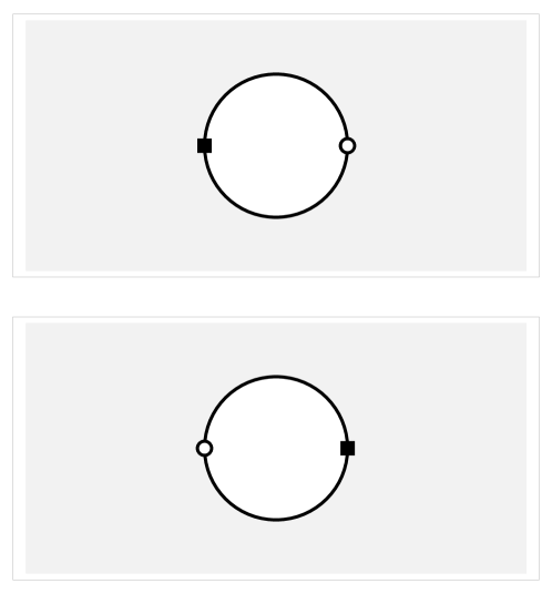
Figure 3: Topology of the spacetime with a single defect wormhole, at $Z_{\pm}=0$ and an arbitrary fixed time $t$. The “upper” ($+$) world is shown by the top panel in this figure and the “lower” ($-$) world by the bottom panel. A single defect wormhole connects the two worlds. Here, the two wormhole mouths are shown as two heavy circles with “antipodal” spacetime points identified (two distinct points on the wormhole mouths are marked by two different symbols, the filled square and the small circle). The “throat” of this particular wormhole has zero length, different from the wormholes sketched in Figures 1 and 2.

3.4 Radial geodesics

From the vacuum-wormhole metric (3.1) with $b_{0}^{2}=\lambda^{2}$, we can get explicitly the radial geodesics $\xi(t)$ passing through the wormhole throat at $\xi=0$:

$$\theta(t)\,\Big{|}^{\text{(K-special)}}_{\text{vacuum\;sol\,;\;rad-geod}} = \pi/2\,,$$ (14a)

$$\phi(t)\,\Big{|}^{\text{(K-special)}}_{\text{vacuum\;sol\,;\;rad-geod}} = 0\,,$$ (14b)

$$\xi(t)\,\Big{|}^{\text{(K-special)}}_{\text{vacuum\;sol\,;\;rad-geod}} = \begin{cases}\pm\,\sqrt{(B\,t)^{2}+2\,B\,\lambda\,t}\,,&\;\;\text{for}\;\;t\geq 0\,,\\[2.84526pt] \mp\,\sqrt{(B\,t)^{2}-2\,B\,\lambda\,t}\,,&\;\;\text{for}\;\;t\leq 0\,,\end{cases}$$ (14c)

with different signs (upper or lower) in front of the square roots for motion in opposite directions and a dimensionless constant $B\in(0,\,1]$.

The radial geodesic (14) with the upper signs has the following trajectory in terms of the Cartesian coordinates (13):

$$Z_{\pm}(t)\,\Big{|}^{\text{(K-special)}}_{\text{vacuum\;sol\,;\;rad-geod}} = 0\,,\qquad\qquad\;\;\text{for}\;\;t\in(-\infty,\,\infty)\,,$$ (15a)

$$Y_{\pm}(t)\,\Big{|}^{\text{(K-special)}}_{\text{vacuum\;sol\,;\;rad-geod}} = 0\,,\qquad\qquad\;\;\text{for}\;\;t\in(-\infty,\,\infty)\,,$$ (15b)

$$X_{-}(t)\,\Big{|}^{\text{(K-special)}}_{\text{vacuum\;sol\,;\;rad-geod}} = -\lambda+B\,t\,,\;\;\;\;\text{for}\;\;t\leq 0\,,$$ (15c)

$$X_{+}(t)\,\Big{|}^{\text{(K-special)}}_{\text{vacuum\;sol\,;\;rad-geod}} = +\lambda+B\,t\,,\;\;\;\;\text{for}\;\;t\geq 0\,,$$ (15d)

with $X_{-}=-\lambda$ and $X_{+}=+\lambda$ identified at $t=0$. The curves in the $(t,\,X_{-})$ and $(t,\,X_{+})$ planes have two parallel straight-line segments, shifted at $t=0$, with equal constant positive slope $B\leq 1$ (velocity magnitude in units with $c=1$); see Figure 4.

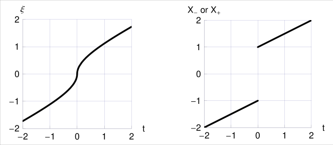
Figure 4: Radial geodesic (14) and (15) with $\lambda=1$ and $B=1/2$.

This equal Minkowski-spacetime velocity before and after the defect crossing is the main argument for using the “antipodal” identification in (13), rather than a “direct” identification on the two 2-spheres $S^{\,2}_{\pm}$, which would correspond to replacing the prefactors $\widetilde{l}$ in (13g) and (13n) by $|\,\widetilde{l}\,|$ and would have a unique spatial orientation (but apparently nonsmooth motion along defect-crossing geodesics). A further argument in favor of the “antipodal” identification, at least for the vacuum case, is given by demanding a smooth solution of the first-order equations of general relativity [8].

3.5 General Ansatz

The special degenerate metric (3.1) can be generalized as follows [8]:

$$ds^{2}\,\Big{|}^{\text{(K-general)}}\equiv g_{\mu\nu}(x)\,dx^{\mu}\,dx^{\nu}\,\Big{|}^{\text{(K-general)}}$$

$$=-e^{2\,\widetilde{\phi}(\xi)}\;dt^{2}+\frac{\xi^{2}}{\xi^{2}+\lambda^{2}}\;d\xi^{2}+\widetilde{r}^{\;2}(\xi)\,\Big{[}d\theta^{2}+\sin^{2}\theta\,d\phi^{2}\Big{]}\,,$$ (16)

with a positive length scale $\lambda$ and real functions $\widetilde{\phi}(\xi)$ and $\widetilde{r}(\xi)$. Again, the coordinates $t$ and $\xi$ range over $(-\infty,\,\infty)$, while $\theta\in[0,\,\pi]$ and $\phi\in[0,\,2\pi)$ are the standard spherical polar coordinates [as mentioned before, we should really use two appropriate coordinate patches for the 2-sphere]. If we assume that $\widetilde{\phi}(\xi)$ remains finite everywhere and that $\widetilde{r}(\xi)$ is positive with $\widetilde{r}(\xi)\sim|\xi|$ for $\xi\to\pm\infty$, then the spacetime from (3.5) corresponds to a wormhole.

If the function $\widetilde{r}(\xi)$ has a global minimum at the value $b_{0}>0$ for $\xi=0$ and if the redshift function $\widetilde{\phi}(\xi)$ is essentially constant near $\xi=0$, then we can expect to obtain nontrivial dynamics for $\lambda^{2}$ values of the order of $b_{0}^{2}$ or larger. As mentioned in Ref. [8], we have once used power series in $\xi^{2}$ for $\widetilde{\phi}(\xi)$ and $\widetilde{r}^{\;2}(\xi)$ and have found energy-momentum components without singular behavior at $\xi=0$. Further work remains to be done.

4 Single Vacuum-Defect Wormhole Revisited

We already have an exact wormhole-type solution of the vacuum Einstein gravitational field equation, as mentioned in the last paragraph of Sec. 3.1 for the special-case metric. Here, we review the vacuum-defect-wormhole solution (abbreviated “vac-def-WH-sol”) in terms of the tetrad and show that it provides a smooth solution [8] of the first-order equations of general relativity. The relevant fields are the tetrad $e^{a}_{\mu}(x)$, which builds the metric tensor $g_{\mu\nu}(x)\equiv e^{a}_{\phantom{z}\mu}(x)\,e^{b}_{\phantom{z}\nu}(x)\,\eta_{ab}$, and the Lorentz connection $\omega^{\phantom{z}a}_{\mu\phantom{z}b}(x)$.

With the differential-form formalism in the notation of Ref. [12] and the definition of the curvature 2-form

$$R^{\,a}_{\,\phantom{z}b}\equiv\text{d}\omega^{\,a}_{\,\phantom{z}b}+\omega^{a}_{\phantom{z}c}\wedge\omega^{c}_{\phantom{z}b}\,,$$ (17)

the first-order vacuum equations of general relativity are explicitly [13]

$$e^{\,[\,a}\wedge D\,e^{\,b\,]} = 0\,,$$ (18a)

$$e^{\,b}\wedge R^{\,cd}\,\epsilon_{abcd} = 0\,,$$ (18b)

where the square brackets around Lorentz indices $a$ and $b$ denote antisymmetrization. Furthermore, $\epsilon_{abcd}$ is the completely antisymmetric symbol and the covariant derivative is defined by $D\,e^{b}\equiv\text{d}e^{b}+\omega^{\,b}_{\,\phantom{z}c}\wedge e^{c}$. The first equation of (18) corresponds to the no-torsion condition and the second to the Ricci-flatness equation.

For the vacuum-defect wormhole, we make the following Ansätze for the dual basis (defined in terms of the tetrad by $e^{a}\equiv e^{a}_{\phantom{z}\mu}\,\text{d}x^{\mu}$) :

$$e^{0}\,\Big{|}_{\text{vac-def-WH-sol}} = \text{d}t\,,$$ (19a)

$$e^{1}\,\Big{|}_{\text{vac-def-WH-sol}} = \frac{\xi}{\sqrt{b^{2}+\xi^{2}}}\;\text{d}\xi\,,$$ (19b)

$$e^{2}\,\Big{|}_{\text{vac-def-WH-sol}} = \sqrt{b^{2}+\xi^{2}}\;\text{d}\theta\,,$$ (19c)

$$e^{3}\,\Big{|}_{\text{vac-def-WH-sol}} = \sqrt{b^{2}+\xi^{2}}\;\sin\theta\;\text{d}\phi\,,$$ (19d)

and for the nonzero components of the connection 1-form:

$$\left\{\omega^{2}_{\phantom{z}1},\,\omega^{3}_{\phantom{z}1},\,\omega^{3}_{\phantom{z}2}\right\}\,\Big{|}_{\text{vac-def-WH-sol}} = \left\{-\omega^{1}_{\phantom{z}2},\,-\omega^{1}_{\phantom{z}3},\,-\omega^{2}_{\phantom{z}3}\right\}\,\Big{|}_{\text{vac-def-WH-sol}}$$ (20)

$$= \left\{\text{d}\theta,\,\sin\theta\;\text{d}\phi,\,\cos\theta\;\text{d}\phi\right\}\,.$$

This particular tetrad and connection are perfectly smooth (in particular, at $\xi=0$) and give a vanishing curvature 2-form:

$$R^{\,a}_{\phantom{z}b}\,\Big{|}_{\text{vac-def-WH-sol}}=0\,,$$ (21)

which corresponds to having the Riemann tensor $\mathcal{R}_{\kappa\lambda\mu\nu}(x)=0$ in the standard coordinate formulation (the calligraphic symbol marks the difference with the curvature 2-form $R^{\,a}_{\phantom{z}b}$).

We can, now, verify that the two first-order vacuum equations in (18) are solved. The first (no-torsion) equation is solved, as it has been used to construct the connection components (20) from the tetrad Ansatz (19). The second (Ricci) equation is trivially solved by (21).

5 Multiple Vacuum-Defect Wormholes

The construction of the multiple-vacuum-defect-wormhole solution (abbreviated “multiple-vac-def-WH-sol”) is straightforward. Here, we only give a brief heuristic discussion and point to Ref. [9] for technical details.

We start by defining the embedding space $M_{\text{embed}}$, which corresponds to the union of two copies of Euclidean 3-space $E_{3}$, one copy being labeled by ‘$+$’ (the “upper” world) and the other by ‘$-$’ (the “lower” world). In each of these 3-spaces, we have standard Cartesian coordinates,

$$M_{\text{embed}} = E_{3}^{\,(+)}\cup\;E_{3}^{\,(-)}$$ (22a)

$$E_{3}^{\,(\pm)} : \left(X_{\pm},\,Y_{\pm},\,Z_{\pm}\right)\;\in\;\mathbb{R}^{3}\,.$$ (22b)

The multiple-vacuum-defect-wormhole solutions only cover part of $M_{\text{embed}}$.

Next, we define $4N$ solution parameters,

$$b_{n} > 0,\,\;\;\;\quad\text{for}\;\;n\in\{1,\,2,\,\ldots\,,\,N\}\,,$$ (23a)

$$\left(\widehat{X}_{n},\,\widehat{Y}_{n},\,\widehat{Z}_{n}\right) \in \mathbb{R}^{3}\,,\quad\text{for}\;\;n\in\{1,\,2,\,\ldots\,,\,N\}\,,$$ (23b)

where $$b_{n} 2\pi n (\widehat{X}_{n},\,\widehat{Y}_{n},\,\widehat{Z}_{n}) B_{n} n b_{n}$$ is the length scale (throat circumference divided by ) of the -th wormhole and are the corresponding center coordinates in the embedding space (equal for lower and upper world). These parameters must be such that balls around the -th center with radius do not touch each other,

$$B_{1}\cap B_{2}\cap\,\ldots\,\cap B_{N} = \emptyset\,.$$ (23c)

The typical size of the wormhole mouths will be denoted by $\overline{b}$ and the typical separation of the wormhole mouths by $\overline{l}$, which is best defined by the average wormhole number density $\overline{n}\equiv 1/\overline{l}^{\,3}$.

Finally, we perform surgery on the embedding space by removing the interiors of the balls $B_{n}$ and identifying “antipodal” points on the respective 2-sphere boundaries, similar to the identification in (13o) with $\lambda$ replaced by $b_{n}$.

This completes the basic construction of the coordinates and a sketch appears in Figure 5 for $N=2$. We now turn to the metric of the multiple-vacuum-defect-wormhole solution.

Between the wormhole mouths, there is the standard flat metric in either 3-space (labelled by $\pm$),

$$ds^{2}\,\Big{|}_{\text{multiple-vac-def-WH-sol}}^{\text{(outside\;WH-mouths)}}=-dt^{2}+\left(dX_{\pm}\right)^{2}+\left(dY_{\pm}\right)^{2}+\left(dZ_{\pm}\right)^{2}\,,$$ (24)

for the spatial coordinates (22b) of the embedding space.

For the metric at or near the wormhole mouths, we have essentially the single-defect-wormhole metric (3.1) for $\lambda=b_{0}=b_{n}$. Specifically, the nearby metric for the particular wormhole mouth with label $\overline{n}$ is given by

$$ds^{2}\,\Big{|}_{\text{multiple-vac-def-WH-sol}}^{\text{(near WH-mouth $\overline{n}$)}}$$

$$=-dt^{2}+\frac{\xi_{\,\overline{n}}^{2}}{b_{\,\overline{n}}^{2}+\xi_{\,\overline{n}}^{2}}\;d\xi_{\,\overline{n}}^{2}+\left(b_{\,\overline{n}}^{2}+\xi_{\,\overline{n}}^{2}\right)\,\Big{[}d\theta_{\,\overline{n}}^{2}+\sin^{2}\theta_{\,\overline{n}}\,d\phi_{\,\overline{n}}^{2}\Big{]}\,,$$ (25)

with coordinates $\xi_{\,\overline{n}}\in[-\Delta_{\,\overline{n}},\,\Delta_{\,\overline{n}}]$ for a positive infinitesimal $\Delta_{\,\overline{n}}\,$, $\theta_{\,\overline{n}}\in[0,\,\pi]$, and $\phi_{\,\overline{n}}\in[0,\,2\pi)$.

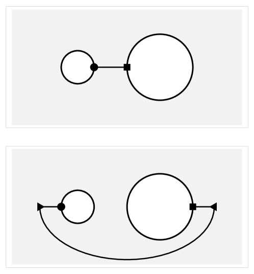
Figure 5: Sketch of the $N=2$ multiple-vacuum-defect-wormhole spacetime, at $Z_{\pm}=0$ and an arbitrary fixed time $t$. The top panel in this figure corresponds to the “upper” world (label ‘$+$’) and the bottom panel to the “lower” world (label ‘$-$’). The two worlds are connected by vacuum-defect wormholes. Here, the wormhole mouths are shown as heavy circles (having radius $b_{1}$ for the left wormhole and $b_{2}$ for the right one) with “antipodal” spacetime points identified (two distinct points are marked by two different symbols, the heavy dot and the filled square). To travel between two particular points of the “lower” world (shown by two different triangles), there is a long way staying in the “lower” world and a short way though the two wormhole throats with a short passage in the “upper” world.

6 Phenomenological Aspects

6.1 Preliminaries

If there is a “gas” of randomly positioned static vacuum-defect wormholes, we would like to measure, or at least bound, the typical wormhole size $\overline{b}$ and the typical wormhole separation $\overline{l}\equiv(\overline{n})^{-1/3}$, defined in terms of the average number density $\overline{n}$. We have shown in Ref. [9] that, different from the case of similar space defects in a single spacetime, vacuum-Cherenkov and scattering bounds on $\overline{b}$ and $\overline{l}$ appear to be rather ineffectual. More successful are imaging bounds, to which we will now turn.

6.2 Imaging bound from an electron microscope

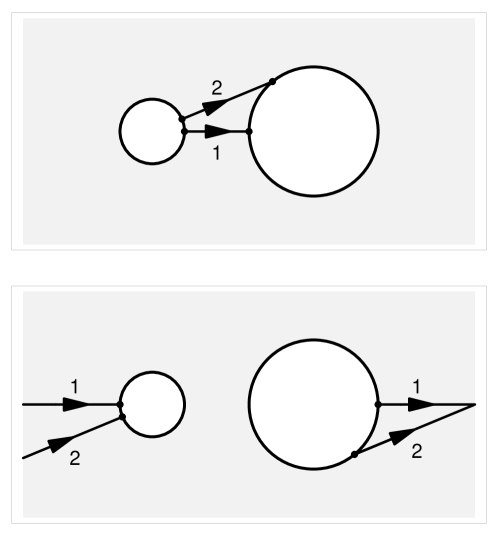
Figure 6: Two light rays in the $N=2$ multiple-vacuum-defect-wormhole spacetime from Figure 5, with a flat metric given by (24) between the wormhole mouths. The light rays start in the “lower” world on the left and the small dots on the wormhole mouths are purely indicative. Both rays re-emerge in the “lower” world after a passage in the “upper” world. The special ray marked “$1$” (connecting the two fictitious wormhole centers) continues straight on, but the other ray marked “$2$” is parallel shifted (here, by a translation to the right with a magnitude equal to twice the wormhole length scale $b_{2}$).

For light travelling a distance $L$, there are $N\sim L/\overline{l}$ encounters with the wormhole mouths. In each encounter, the ray is typically parallel shifted by an amount of order $\pm b_{n}$, which is illustrated in Figure 6 for a single pair of wormholes ($N=2$). As explained in Sec. IV B of Ref. [9], the built-up parallel shift of the light ray results from a random-walk process and its order of magnitude is given by

$$[\Delta x]_{\text{random-walk}}\sim\sqrt{N}\,\overline{b}\sim\left(\,\overline{b}/\overline{l}\,\right)\;\sqrt{L\,\overline{l}}\,.$$ (26)

In order to get a clear image of a 2D sample with substructure $[\delta x]_{\text{sample}}$, we must have negligible random-walk parallel shifts of the light ray,

$$[\Delta x]_{\text{random-walk}}\lesssim[\delta x]_{\text{sample}}\,,$$ (27)

where the inequality should perhaps be stronger (with ‘$\lesssim$’ replaced by ‘$\ll$’), but we prefer to remain conservative.

Instead of light rays we can also consider electron beams in a transmission electron microscope (TEM); see, e.g., Ref. [14] for some background. A special-purpose TEM would have condenser lenses designed to produce more or less parallel rays after the rays have passed through a 2D sample with subångström structure. Furthermore, these parallel rays just after the 2D sample must travel freely for about $L\sim 10\,\text{cm}$ (possibly broadened by vacuum-defect-wormhole effects) before they enter the rest of the microscope. If this experimental setup could indeed be realized and if clear images would be obtained, then the following bound would result [9]:

$$\left(\,\overline{b}/\overline{l}\,\right)\;\overline{b}\;\Big{|}^{\text{(special-TEM)}}\lesssim\frac{\left([\delta x]_{\text{sample}}\right)^{2}}{L}=10^{-21}\,\text{m}\;\left(\frac{[\delta x]_{\text{sample}}}{0.1\,\text{\r{A}}}\right)^{2}\,\left(\frac{0.1\,\text{m}}{L}\right)\,,$$ (28)

where (26) and (27) have been used.

Bound (28), for the $[\delta x]_{\text{sample}}$ and $L$ values stated, is perfectly consistent with having a gas of Planck-scale vacuum-defect-wormholes, $\,\overline{b}\sim\overline{l}\sim 10^{-35}\,\text{m}$.

6.3 Backward time travel

It was pointed out in Morris–Thorne’s landmark paper [7] that traversable exotic-matter wormholes appear to allow for backward time travel. An alternative procedure for getting a time machine was suggested by Frolov and Novikov [15]. These last authors propose to insert a large point mass near one of the mouths of an intra-universe traversable exotic-matter wormhole, so that a clock near that mouth runs slower than a clock near the other mouth and a time machine appears after a sufficiently long time.

A similar time machine can be constructed by use of multiple vacuum-defect wormholes and a single localized mass [9]. Essentially, there are two steps.

In the first step, we observe that a pair of vacuum-defect wormholes can act as a single intra-universe wormhole. Consider, namely, a point (left triangle) in the lower world near the heavy dot of the bottom panel in Figure 5. While staying in the lower world, it is possible to travel along a long path to a point (right triangle) near the filled square on the right (see the ellipse segment between the two triangles in the bottom panel of Figure 5). Alternatively, it is possible, in the lower world, to enter the left wormhole at the heavy dot, to emerge in the upper world at the heavy dot, to travel in the upper world along a short straight line towards the filled square, to enter the right wormhole at the filled square, and, finally, to re-emerge in the lower world at the filled square.

In the second step, we position, for an identical wormhole pair (Figure 5 but now with open symbols, the open square and the small circle), a static point mass in the lower world just to the right of the open square in the bottom panel of the modified Figure 5. Now, a lower-world clock near the open square runs slower (gravitational redshift) than a lower-world clock near the small circle. Recall that the gravitational-redshift effect follows directly from the equivalence principle; see, e.g., Sec. 7.4 of Ref. [16].

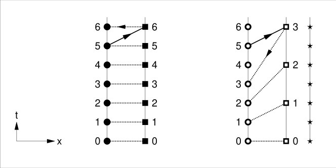
Figure 7: Spacetime-diagram sketches (in rescaled units) of four identical lower-world clocks near the four wormhole mouths of two identical vacuum-defect-wormhole pairs. The figure explains the appearance of a time machine for the vacuum-defect-wormhole pair on the right with an added lower-world static point mass (star) near the right wormhole mouth (open square); see Sec. 6.3 for a detailed description.

After these two steps, the time machine appears automatically and an illustration is given by Figure 7. As said, take two identical vacuum-defect-wormhole pairs (the first pair with the heavy dot and the filled square in the bottom panel of Figure 5 and the second pair from the same figure but now with open symbols). Introduce four identical lower-world clocks, at rest near the four wormhole mouths. Next, consider two paths starting at the left triangle in the bottom panel of Figure 5 and ending at the right triangle in the bottom panel: the long path (ellipse segment) that remains entirely in the lower world and the short path that first enters the left wormhole, runs in the upper world towards the right wormhole, enters the right wormhole, and re-emerges in the lower world. In order to streamline the further discussion, we move the left triangle in Figure 5 close to the heavy dot and the right triangle close to the filled square. Also, we push the two wormholes together, so that the straight path in the upper world is negligibly short compared to the long path in the lower world.

Without adding a point mass (left wormhole pair in Figure 7), both clocks run at the same rate and the ticks are shown for $t_{\text{left}}=t_{\text{right}}=0,\,1,\,\ldots\,,\,6$. An ultrafast explorer starts out at local time $t_{\text{left}}=5$ from a point near the left wormhole mouth (heavy dot) on the long path in the lower world (full line with arrow in the spacetime diagram on the left) to reach a point near the right wormhole mouth (filled square) and then passes quickly through the two wormhole throats (dotted line with arrow in the spacetime diagram on the left) back to the starting point (heavy dot) at local time $t_{\text{left}}=6$.

With a static point mass added (shown by a star for the right wormhole pair in Figure 7), the clock near the right wormhole mouth (open square) runs slower than the clock near the left wormhole mouth (small circle). Again, an explorer starts out at local time $t_{\text{left}}=5$ from a point near the left wormhole mouth (small circle) on the long path in the lower world (full line with arrow in the spacetime diagram on the right) to reach a point near the right wormhole mouth (open square) and then passes quickly through the two wormhole throats (dotted line with arrow in the spacetime diagram on the right) back to the starting point (small circle) at local time $t_{\text{left}}=3$. In other words, the explorer has travelled back in time ($t_{\text{left,\,return}}=3$ being less than $t_{\text{left,\,start}}=5$) and effectively a time machine is operating. In fact, the time machine starts working for departure times $t_{\text{left}}\geq 1$ (the same explorer leaving at local time $t_{\text{left}}=1$ returns at local time $t_{\text{left}}=1$). For earlier departure times $t_{\text{left}}<1$, the return is at a later time $t_{\text{left}}$. For example, if the same traveller leaves at $t_{\text{left}}=0$, then the return will be at $t_{\text{left}}=1/2$.

This simple example shows that, in principle, a time machine can appear if there exists one pair of vacuum-defect wormholes and a single point mass which can be freely positioned in either of the two worlds. Whether or not this time machine without exotic matter is stable (classically and quantum mechanically) remains to be seen. Obviously, backward time travel is hard to swallow and we refer to, e.g., Ref. [17] for further discussion.

7 Final Remarks

The vacuum-defect-wormhole solution (19) and (20) has a length scale $\lambda$ as a free parameter. If there is a preferred value $\overline{\lambda}$ in the actual Universe, then that value can only come from a theory beyond general relativity.

One such theory could be nonperturbative superstring theory in a matrix-model realization. We have explicitly considered the Ishibashi–Kawai–Kitazawa–Tsuchiya (IKKT) matrix model [18], also known as IIB matrix model [19]. That matrix model could indeed give rise to an emergent spacetime with or without spacetime defects [20, 21]. If defects do appear, then the typical length scale $\overline{\lambda}$ of a remnant vacuum-wormhole defect would be related to the IIB-matrix-model length scale $\ell$. The Planck length $l_{P}\equiv G^{1/2}$ would also be related to $\ell$. Combined, this suggests that the typical vacuum-defect-wormhole length scale $\overline{\lambda}$ might be of the order of the Planck length $l_{P}\sim 10^{-35}\,\text{m}$.

At this moment, we do not have experimental bounds which rule out a “gas” of Planck-scale vacuum-defect wormholes (Sec. 6.2). For such Planck-scale wormholes, the appearance of backward time travel (Sec. 6.3) is perhaps acceptable.

If it is now possible to “harvest” such Planck-scale vacuum-defect wormholes and to “fatten” them by adding a finite amount of normal matter (as suggested by the results of App. B in Ref. [8]), then we may have to live up to the possibility of having time machines for human-scale robots (and possibly humans themselves). But all this is admittedly still very far off in the future, if at all realistic.

Note Added

An interesting extension of the vacuum-defect-wormhole solution has been suggested recently by Wang [22]. His suggestion is to add a Schwarzschild-type factor $\big{[}1-2M/\sqrt{b^{2}+\xi^{2}}\,\big{]}^{1/2}$ to the dual-basis component (19a) and the inverse factor to the dual-basis component (19b), where the parameter $M<|b|/2$ can be positive or negative. The corresponding spin-connection 1-form $\omega^{a}_{\phantom{z}b}$ follows directly from the no-torsion condition (18a). These extended Ansätze for the tetrad and connection then solve the Ricci-flatness equation (18b), as shown in App. B of Ref. [22].

This mathematical result is more or less obvious, but the physical interpretation is less clear. In the original Schwarzschild vacuum metric, we interpret $M$ as a point mass sitting at $r=0$, where the vacuum metric no longer holds. But what is the physics of $M$ in the extended-vacuum-defect-wormhole spacetime? There appears to be no place for the matter, as the manifold is geodesically complete. One possible interpretation may be that a nonzero $M$ in the 4-dimensional metric describes higher-dimensional effects.

References

- [1] A. Einstein (1916) Die Grundlage der allgemeinen Relativitätstheorie (The foundation of the general theory of relativity). Annalen Phys. (Leipzig) 49 769–822.
- [2] A. Einstein, N. Rosen (1935) The particle problem in the general theory of relativity. Phys. Rev. 48 73–79.
- [3] J.A. Wheeler (1955) Geons. Phys. Rev. 97 511–536.
- [4] J.A. Wheeler (1968) Superspace and the nature of quantum geometrodynamics. In: C.M. DeWitt, J.A. Wheeler (eds) “Battelle Rencontres 1967”. Benjamin, New York, USA, pp. 242-307.
- [5] H.G. Ellis (1973) Ether flow through a drainhole: A particle model in general relativity. J. Math. Phys. 14 104–117.
- [6] K.A. Bronnikov (1973) Scalar-tensor theory and scalar charge. Acta Phys. Polon. B 4 251–266.
- [7] M.S. Morris, K.S. Thorne (1988) Wormholes in space-time and their use for interstellar travel: A tool for teaching general relativity. Am. J. Phys. 56 395–412.
- [8] F.R. Klinkhamer (2023) Defect wormhole: A traversable wormhole without exotic matter. Acta Phys. Polon. B 54 5-A3; [arXiv:2301.00724].
- [9] F.R. Klinkhamer (2023) Vacuum defect wormholes and a mirror world. [arXiv:2305.13278].
- [10] F.R. Klinkhamer (2019) Regularized big bang singularity. Phys. Rev. D 100 023536; [arXiv:1903.10450].
- [11] E.I. Guendelman, A. Kaganovich, E. Nissimov, S. Pacheva (2009) Einstein-Rosen ‘bridge’ needs lightlike brane source. Phys. Lett. B 681 457–462; [arXiv:0904.3198].
- [12] T. Eguchi, P.B. Gilkey, A.J. Hanson (1980) Gravitation, gauge theories and differential geometry. Phys. Rept. 66 213–393.
- [13] G.T. Horowitz (1991) Topology change in classical and quantum gravity. Class. Quant. Grav. 8 587–601.
- [14] J.C.H. Spence (2017) “High-Resolution Electron Microscopy, 4th Edition”. Oxford University Press, Oxford, UK.
- [15] V.P. Frolov, I.D. Novikov (1990) Physical effects in wormholes and time machines. Phys. Rev. D 42, 1057–1065.
- [16] C.W. Misner, K.S. Thorne, J.A. Wheeler (2017) “Gravitation”. Princeton University Press, Princeton, NJ, USA.
- [17] M. Visser (1996) “Lorentzian Wormholes: From Einstein to Hawking”. Springer, New York, NY, USA.
- [18] N. Ishibashi, H. Kawai, Y. Kitazawa, A. Tsuchiya (1997) A large- reduced model as superstring. Nucl. Phys. B 498 467–491; [arXiv:hep-th/9612115].
- [19] H. Aoki, S. Iso, H. Kawai, Y. Kitazawa, A. Tsuchiya, T. Tada (1999) IIB matrix model. Prog. Theor. Phys. Suppl. 134 47–83; [arXiv:hep-th/9908038].
- [20] F.R. Klinkhamer (2021) IIB matrix model: Emergent spacetime from the master field. Prog. Theor. Exp. Phys. 2021 013B04; [arXiv:2007.08485].
- [21] F.R. Klinkhamer (2022) IIB matrix model, bosonic master field, and emergent spacetime. PoS CORFU2021 259; [arXiv:2203.15779].
- [22] Z.L. Wang (2023) On a Schwarzschild-type defect wormhole. [arXiv:2307.01678].