Optimal Robot Path Planning In a Collaborative Human-Robot Team
with Intermittent Human Availability

Abstract

This paper presents a solution for the problem of optimal planning for a robot in a collaborative human-robot team, where the human supervisor is intermittently available to assist the robot in completing tasks more quickly. Specifically, we address the challenge of computing the fastest path between two configurations in an environment with time constraints on how long the robot can wait for assistance. To solve this problem, we propose a novel approach that utilizes the concepts of budget and critical departure times, which enables us to obtain optimal solution while scaling to larger problem instances than existing methods. We demonstrate the effectiveness of our approach by comparing it with several baseline algorithms on a city road network and analyzing the quality of the obtained solutions. Our work contributes to the field of robot planning by addressing a critical issue of incorporating human assistance and environmental restrictions, which has significant implications for real-world applications.

I Introduction

Robots have come a long way in the past decades, with increasing levels of autonomy transforming the way they operate in various domains, from factories and warehouses to homes and public spaces [1, 2, 3]. However, navigating dynamic environments effectively continues to be a formidable challenge. Despite the significant strides made in robot autonomy, human oversight remains vital in enhancing safety, efficiency or to comply with regulatory requirements. For example, a robot navigating through an urban environment must abide by traffic regulations and may require human assistance in busy or construction areas to ensure safety or expedite operations. Similarly, in an exploration task, robots may require replanning due to changes in the environment, while the supervisor has already committed to a supervision schedule for other robots and is only intermittently available. By considering the operator’s availability and environmental restrictions, robots can plan their paths more efficiently, avoid unnecessary waiting and decide when to use human assistance. Figure 1 shows the problem overview with an example of a robot navigating in a city. However, the presented problem can be generalized to any arbitrary task which can be completed via different sub-tasks defined using precedence and temporal constraints.

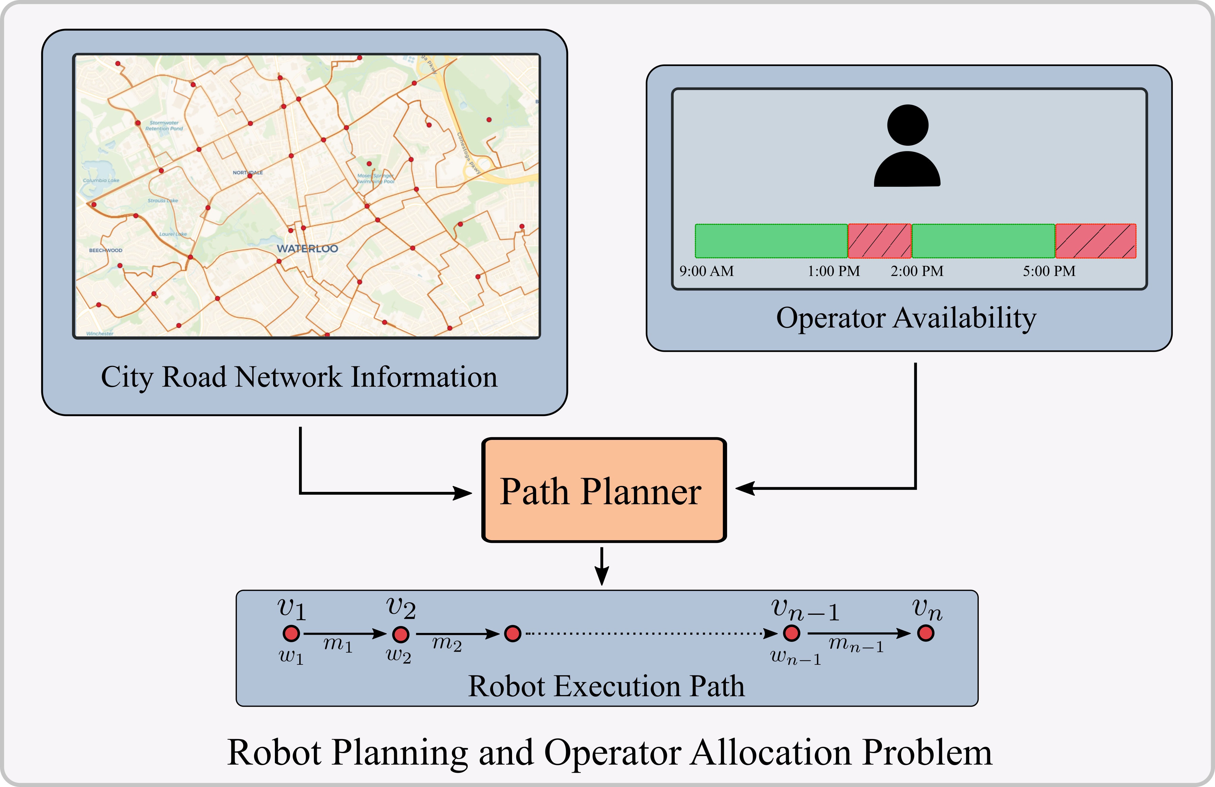
Figure 1: Problem Overview: Given the information of a city road network with speed and waiting restrictions, and the availability of human assistance, the objective is to determine a path that results in the fastest arrival at a goal location. The path consists of three components: (1) the vertices or locations to navigate through, denoted as $(v_{1},v_{2},\ldots,v_{n})$; (2) the amount of waiting required at intermediate locations, denoted as $(w_{1},w_{2},\ldots,w_{n-1})$; and (3) whether to use human assistance, denoted as $(m_{1},m_{2},\ldots,m_{n-1})$. In this paper, we propose a novel and efficient planning algorithm to obtain the required path.

We consider the problem of robot planning with the objective of finding the fastest path between two configurations. We demonstrate our approach through an example of robot navigation in an urban environment with intermittent operator availability, varying travel speeds, and waiting limits. Specifically, we consider a city road network where the robot can traverse through different locations either autonomously or with the assistance of a human supervisor, each taking different amounts of time. However, the supervisor is only available at certain times, and the robot has a limited amount of time to wait at a location before it must move on to its next destination. By formulating the problem in this way, we aim to address the challenge of collaborative robot planning in real-world environments where the availability of human supervisors may be limited and thus can affect the optimal route for the robot. In this paper, we present a method to compute the fastest path from one location to another while accounting for all these constraints.

The problem of robot path planning with operator allocation in dynamic networks is inspired by real-world scenarios where the availability of human assistance and thus the robot’s speed of travel and its ability to traverse certain paths can change over time, e.g., [4]. Traditional methods, such as time-dependent adaptations of the Dijkstra’s algorithm, are not designed to handle situations in dynamic environments where waiting is limited, and the task durations may not follow the first-in-first-out (FIFO) property [5]. This means that a robot may arrive at its target location earlier by departing later from its previous location, for example, by using human assistance. To address these challenges, we draw on techniques from the time-dependent shortest path literature to solve the problem. Unfortunately, existing optimal solution techniques are severely limited by their computational runtime. In this paper, we propose a novel algorithm that is guaranteed to find optimal solution and runs orders of magnitude faster than existing solution techniques.

Contributions: Our main contributions are as follows:

1) We propose a novel graph search algorithm for the collaborative planning problem with intermittent human availability. The algorithm operates by intelligently selecting the times of exploration and by combining ranges of arrival times into a single search node.

2) We provide the proof that the algorithm generates optimal solutions.

3) We demonstrate the effectiveness of our approach in a city road-network, and show that it outperforms existing approaches in terms of computational time and/or solution quality.

II Background and Related Work

In this section, we discuss some relevant studies from the existing literature in the area of robot planning with human supervision/collaboration. We also look into how the presented problem can be solved using existing techniques from related fields.

Planning with Human Collaboration: The problem of task allocation and path planning for robots operating in collaboration with humans has been studied extensively in recent years. Researchers have proposed various approaches, such as a data-driven approach for human-robot interaction modelling that identifies the moments when human intervention is needed [6], and a probabilistic framework that develops a decision support system for the human supervisors, taking into account the uncertainty in the environment [7]. In the context of autonomous vehicles, studies have investigated cooperative merging of vehicles at highway ramps [8] and proposed a scheduling algorithm for multiple robots that jointly optimize task assignments and human supervision [9].

Task allocation is a common challenge in mixed human-robot teams across various applications, including manufacturing [10], routing [11], surveying [12], and subterranean exploration [4]. In addition, the problem of computing the optimal path for a robot under time-varying human assistance bears similarity to queuing theory applications, such as optimal fidelity selection [13] and supervisory control of robots via a multi-server queue [14]. These studies provide insights into allocating assistance and path planning for robots in collaborative settings, but do not address our specific problem of computing the optimal path for a robot under bounded waiting and intermittent assistance availability. Additionally, our problem differs in that the robot can operate autonomously even when assistance is available, i.e., the collaboration is optional.

Time-Dependent Shortest Paths: The presented problem is also related to time-dependent shortest path (TDSP) problems, which aim to find the minimum cost or minimum length paths in a graph with time-varying edge durations [5, 15]. Existing solution approaches include planning in graphs with time-activated edges [5], implementing modified $A^{*}$ [16], and finding shortest paths under different waiting restrictions [17, 18]. Other studies have explored related problems such as computing optimal temporal walks under waiting constraints [19], and minimizing path travel time with penalties or limits on waiting [20]. Many studies in TDSP literature have addressed the first-in-first-out (FIFO) graphs [5], while others have explored waiting times in either completely restricted or unrestricted settings. However, the complexities arising from non-FIFO properties, bounded waiting and the need to make decisions on the mode of operation, i.e., autonomous or assisted, have not been fully addressed in the existing literature [20, 21, 18].

The most relevant solution technique that can be used to solve our problem is presented in [22], which solves a TDSP problem where the objective is to minimize the path cost constrained by the maximum arrival time at the goal vertex. This method iteratively computes the minimum cost for all vertices for increasing time constraint value. A time-expanded graph search method [23] is another way of solving the presented problem by creating separate edges for autonomous and assisted modes. We discuss these two methods in more detail in Sec. VI. As we will see, the applicability of these solution techniques to our problem is limited due to their poor scalability for large time horizons and increasing graph size.

III Problem Definition

The problem can be defined as follows. We are given a directed graph $G=(V,E)$, modelling the robot environment, where each edge $e\in E$ has two travel times corresponding to the two modes of operation: an autonomous time $\tau(e,0)$ and an assisted time $\tau(e,1)$, with the assumption that $\tau(e,0)\geq\tau(e,1)$. When starting to traverse an edge, the robot must select the mode of operation for the traversal that is used for the entire duration of the edge. While the autonomous mode is always available, the assisted mode can only be selected if the supervisor is available for the entire duration of the edge (under assisted mode). The supervisor’s availability is represented by a binary function $\mu$, with $\mu([t_{1},t_{2}])=1$ indicating availability during the time window $[t_{1},t_{2}]$, and 0 otherwise. Additionally, at each vertex $v\in V$, the robot can wait for a maximum duration of $\overline{w}_{v}\geq 0$ before starting to traverse an outgoing edge.

The robot’s objective is to determine how to travel from a start vertex to a goal vertex. This can be represented as an execution path $\mathcal{P}$, specified as a list of edges to traverse, the amount of waiting required at intermediate vertices and the mode of operation selected for each edge. The objective of this problem is to find an execution path (or simply path) from a start vertex $s\in V$ to a goal vertex $g\in V\setminus\{s\}$, such that the arrival time at $g$ is minimized.

Given a set $\hat{\mathcal{P}}$ of all possible paths $\mathcal{P}$ of arbitrary length $n$, such that $\mathcal{P}\coloneqq\langle(v_{1},t_{1},w_{1},m_{1}),(v_{2},t_{2},w_{2},m_{2}),\ldots,$ $(v_{n},t_{n},w_{n},m_{n})\rangle$, we can write the problem objective as follows:

$$\min_{\mathcal{P}\in\hat{\mathcal{P}}}\;\;\;\quad \;t_{n}$$

$$s.t.\quad v_{1} =s,\;v_{n}=g$$

$$e_{v_{i}v_{i+1}} \in E\;\,\qquad\quad\forall~{}i\in[1,n-1]$$

$$t_{i+1} =t_{i}+w_{i}+\tau(e_{v_{i}v_{i+1}},m_{i})\quad\forall~{}i\in[1,n-1]$$

$$w_{i} \leq\overline{w}_{v_{i}}\;\,\,\quad\quad\forall~{}i\in[1,n-1]$$

$$m_{i}=1 \Rightarrow\mu([t_{i}+w_{i},t_{i+1}])=1\;\;\;\quad\forall~{}i\in[1,n-1].$$

The first constraint ensures that the path starts at $s$ and ends at $g$. The second constraint ensures that the topological path is valid in the graph. The third constraint ensures that the path does not violate travel duration requirements at any edge. Fourth constraint ensures that the waiting restrictions are met at each vertex. Finally, the fifth condition ensures that an edge can only be assisted if the operator is available at least until the next vertex is reached.

To efficiently solve this problem, we must make three crucial decisions: selecting edges to travel, choosing the mode of operation, and determining the waiting time at each vertex. Our proposed method offers a novel approach to computing the optimal solution. However, before delving into the details of our solution, it is necessary to grasp the concept of budget and how new nodes are generated during the search process.

IV Budget and Node Generation

Since the robot is allowed to wait (subject to the waiting limits), it is possible to delay the robot’s arrival at a vertex by waiting at one or more of the preceding vertices. Moreover, the maximum amount of time by which the arrival can be delayed at a particular vertex depends on the path taken from the start to that vertex. Our key insight is that this information about the maximum delay can be used to efficiently solve the given problem by removing the need to examine the vertices at every possible arrival time. We achieve this by augmenting the search space into a higher dimension, using additional parameters with the vertices of the given graph. A node in our search is defined as a triplet $(x,a_{x},b_{x})$, corresponding to a vertex $x\in V$, arrival time $a_{x}\in\mathbb{Z}_{\geq 0}$ and a budget $b_{x}\in\mathbb{Z}_{\geq 0}$. The budget here defines the maximum amount of time by which the arrival at the given vertex can be delayed. Thus, the notion of budget allows a single node $(x,a_{x},b_{x})$ to represent a range of arrival times from $[a_{x},a_{x}+b_{x}]$ at vertex $x$. Therefore, the allowed departure time from this vertex lies in the interval $[a_{x},a_{x}+b_{x}+\overline{w}_{x}]$.

IV-A Node Generation

The proposed algorithm is similar to standard graph search algorithms, where we maintain a priority search queue, with nodes prioritized based on the earliest arrival time (plus any admissible heuristic). Nodes are then extracted from the queue, their neighbouring nodes are generated and are added to the queue based on their priority. Since in our search a node is defined by the vertex, arrival time and budget, we must determine these parameters for the newly generated nodes when exploring a given node. To characterize the set of nodes to be generated during the graph search in our proposed algorithm, we define the notion of direct reachability as follows.

Definition 1 (Direct reachability).

A node $(y,a_{y},b_{y})$ is said to be directly reachable from a node $(x,a_{x},b_{x})$ if $x$ and $y$ are connected by an edge, i.e., $e_{xy}\in E$, and it is possible to achieve all arrivals times in $[a_{y},a_{y}+b_{y}]$ at $y$ through edge $e_{xy}$ for some departure time $t_{D}\in[a_{x},a_{x}+b_{x}+\overline{w}_{x}]$ from $x$ and some mode of travel.

As an example, consider a node $(x,10,2)$ with $\tau(e_{xy},0)=5$ and $\overline{w}_{x}=3$. Then the nodes $(y,15,5),(y,16,4)$ and $(y,17,3)$ are a few directly reachable nodes from $(x,10,2)$ (corresponding to departure times $10$, $11$ and $12$, respectively).

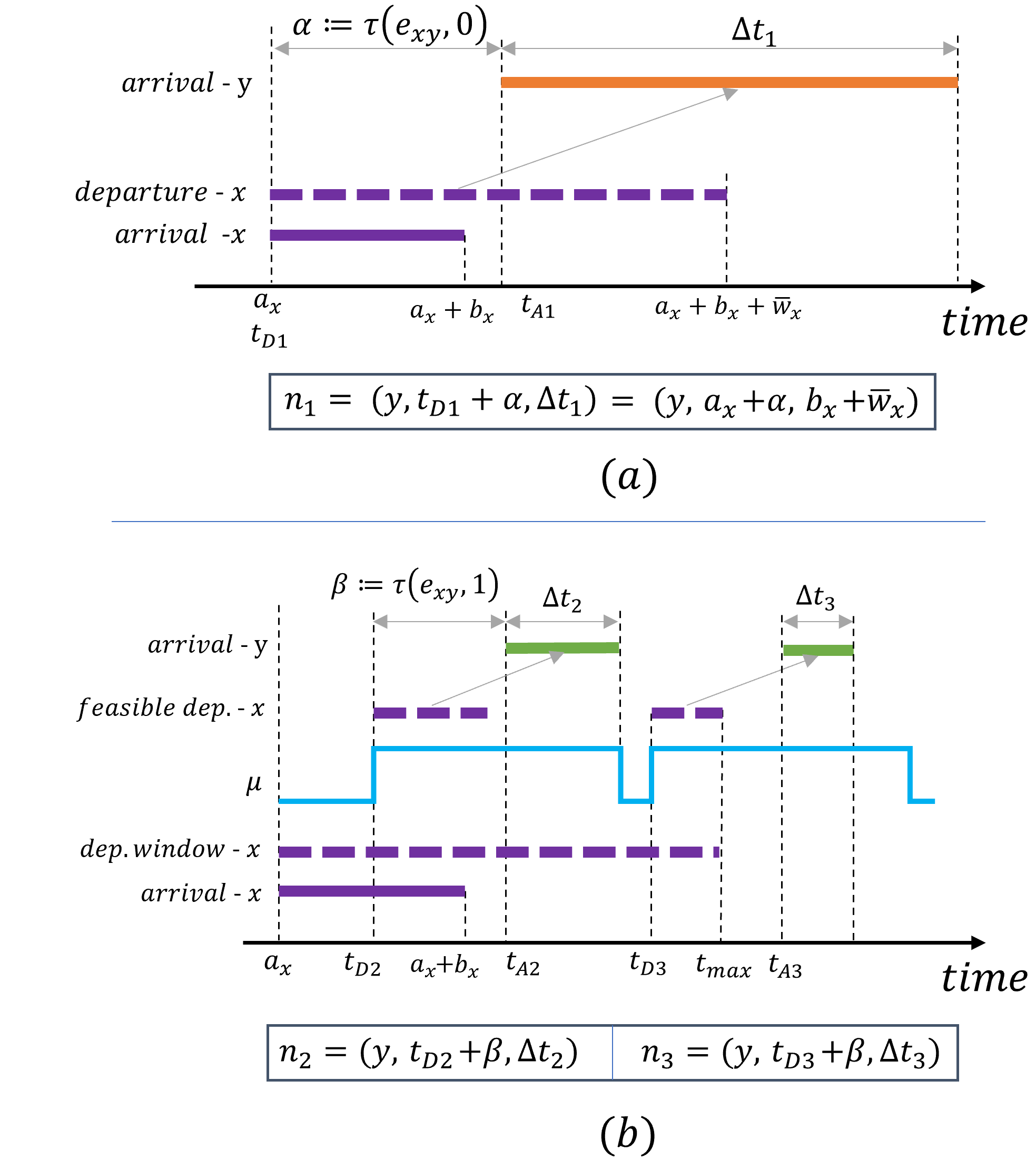
Figure 2: An example explaining the notion of budget and determining the resulting node when a node $(x,a_{x},b_{x})$ is explored. (a) Under autonomous mode, the earliest departure from $x$ is $a_{x}$ (i.e., no waiting). Since autonomous mode is always available to the robot, the corresponding arrival time at $y$ forms a single block, shown as a solid orange line. This can be thus represented using a single node $n_{1}$. (b) Under the assisted mode, feasible departure times from $x$ are governed by the operator availability function $\mu$, and a time $t_{max}=\min(\alpha-\beta,b_{x},\overline{w}_{x})$. In this example, the resulting arrival time at $y$ forms two separate blocks, shown as solid green lines on the time axis. Thus, exploring the node under assisted operation generates two nodes, $n_{2}$ and $n_{3}$.

Like standard graph search methods, our algorithm aims to generate all nodes directly reachable from the current node during the exploration process. One approach is to generate all directly reachable nodes from the given node $(x,a_{x},b_{x})$ for all possible departure times in $[a_{x},a_{x}+b_{x}+\overline{w}_{x}]$. However, this results in redundancy when multiple nodes can be represented collectively using a single node with a suitable budget.

As the operator availability changes, the possible arrival times at the next vertex may present themselves as separate blocks of time. A block of arrival times can be represented using a single node, and thus we only need to generate a new node for each arrival time block. To understand this, we consider the example given in Fig. 2, where a node $(x,a_{x},b_{x})$ is being extracted from the queue, and we want to generate the nodes corresponding to a neighbouring vertex $y$. The arrival time range at $x$, $[a_{x},a_{x}+b_{x}]$ is shown as solid purple line. The possible departure window $[a_{x},a_{x}+b_{x}+\overline{w}_{x}]$ is shown as purple dashed line.

Under autonomous operation, the edge can be traversed by departing at any time in the departure window, resulting in possible arrival time at vertex $y$ in the interval $[a_{x}+\alpha,a_{x}+b_{x}+\overline{w}_{x}+\alpha]$, shown as solid orange line. Therefore, we can represent these possible arrival times using the node $n_{1}=(y,a_{x}+\alpha,b_{x}+\overline{w}_{x})$, where $a_{x}+\alpha$ is the earliest arrival time at $y$ and $b_{x}+\overline{w}_{x}$ is the new budget. Note that the new budget is increased from the previous value by an amount of $\overline{w}_{x}$.

Under assisted operation, only a subset of departure window is feasible, as shown in Fig. 2(b). This results in separate blocks of arrival times at $y$, shown as solid green lines. The range of arrival times corresponding to these blocks become the budget values for the new nodes. In the given example, two nodes are generated: $n_{2}=(y,t_{D2}+\beta,\Delta t_{2})$ and $n_{3}=(y,t_{D3}+\beta,\Delta t_{3})$.

Note that the feasible departure times are limited by operator availability and $t_{max}$. The value of $t_{max}$ is the minimum of $b_{x}+\overline{w}_{x}$ and $\alpha-\beta$. The former quantity limits the departure from $x$ to $a_{x}+b_{x}+\overline{w}_{x}$, while the latter comes from the observation that any departure time $t_{D}>a_{x}+(\alpha-\beta)$ will result in arrival at $y$ at a time $a_{y}>a_{x}+\alpha$, and a budget $b_{y}<b_{x}+\overline{w}_{x}$. However, this arrival time range is already covered by the node generated under autonomous operation.

Critical departure times: Note that the earliest arrival times for each of the three new nodes correspond to unique departure times from $x$ ($t_{D1},t_{D2},t_{D3}$ in Fig. 2). We refer to these times as critical departure times, as exploring a node only at these times is sufficient to generate nodes that cover all possible arrival times at the next vertex. Since in the presented problem, the edge duration depends on the mode of operation selected, the set of critical departure times for a node is a subset of times when the operator availability changes, and thus can be efficiently determined.

Next, we present how these concepts are used by our proposed Budget-$A^{*}$ algorithm to solve the given problem.

V Budget $A^{*}$ Algorithm

This section details the proposed Budget $A^{*}$ algorithm and its three constituent functions: EXPLORE, REFINE and GET-PATH. To recall, a node in our search is defined as a tuple $(x,a_{x},b_{x})$. A pseudo-code for the Budget-$A^{*}$ algorithm is given in Alg. 1, and more details on the constituent functions follow.

1:  Input: $G=(V,E),\tau,\mu,\overline{w},s,g$

2:  $Q\leftarrow\text{initialize priority queue}$

3:  $S\leftarrow\emptyset$

4:  $Q.\text{push}((s,0,0))$

5:  $\psi(x,a)\leftarrow nil$ for all $x\in V,a\in\mathbb{Z}_{\geq 0}$ // Initialize predecessor function

6:  while $Q$ not empty do

7:     $\scalebox{0.9}[1.0]{{currNode}}\coloneqq(x,a_{x},b_{x})\leftarrow Q.\text{extract-min}()$

8:     $S\leftarrow S\cup\scalebox{0.9}[1.0]{{currNode}}$

9:     if $x=g$ then

10:        break

11:     for all $y\in\text{neighbors}(x)$ do

12:        $\mathcal{N}\leftarrow\text{EXPLORE}(a_{x},b_{x},\overline{w}_{x},e_{xy},\tau,\mu)$

13:        for all $(y,a_{i},b_{i},m_{i})\in\mathcal{N}$ do

14:           $\scalebox{0.9}[1.0]{{newNode}}\leftarrow(y,a_{i},b_{i})$

15:           $Q,\psi\leftarrow\text{REFINE}(Q,\scalebox{0.9}[1.0]{{newNode}},\scalebox{0.9}[1.0]{{currNode}},\psi,m_{i})$

16:  $path\leftarrow\text{GET-PATH}(\scalebox{0.9}[1.0]{{currNode}},\overline{w},\psi,\tau)$

Algorithm 1 Budget $A^{*}$

The algorithm initializes an empty priority queue $Q$, a processed set $S$ and a predecessor function $\psi$. It then adds a node $(s,0,0)$ to $Q$ denoting an arrival time of exactly $0$ at $s$. The algorithm iteratively extracts the node with the earliest arrival time (plus an admissible heuristic) from $Q$, adds it to $S$, and generates new candidate nodes for each of its neighbors using the EXPLORE function. The REFINE function then checks if these nodes can be added to the queue, removes redundant nodes from $Q$, and updates predecessor information. The algorithm continues until $Q$ is empty or the goal vertex is reached. The GET-PATH function generates the required path using the predecessor data and waiting limits.

V-A Exploration

The EXPLORE function takes in several input parameters: arrival time $a_{x}$, budget $b_{x}$, waiting limit $\overline{w}_{x}$, edge $e_{xy}$, travel durations $\tau$ and operator availability $\mu$. The function returns a set $\mathcal{N}$ of candidate nodes of the form $(y,a_{i},b_{i},m_{i})$, where $a_{i},b_{i},m_{i}$ are the arrival time, budget and the mode of operation respectively, corresponding to all critical departure times from the node $(x,a_{x},b_{x})$ to vertex $y$. A pseudo-code is shown in Alg. 2.

As discussed in Sec. IV, the autonomous mode generates one new node, while assisted mode can generate multiple nodes depending on operator availability, node budget and task duration. The function first adds a node $(y,a_{x}+\alpha,b_{x}+\overline{w}_{x})$ corresponding to the autonomous mode to $\mathcal{N}$.

For the assisted mode, it first computes the maximum useful delay in departure $t_{max}$. Next, it generates an ordered set $\mathcal{F}$ of feasible departure times from the current node as the times in departure window when it’s possible to depart under assisted mode, computed using $\mu$ and $\beta$ (line 5). Lines 7-8 generate a new node $(y,a_{y},b_{y})$ for each critical departure time $t_{d}$, with a budget $b_{y}=0$ and arrival time $a_{y}=t_{d}+\beta$. The budget is then incremented for each consecutive departure time in $\mathcal{F}$. A gap in $\mathcal{F}$ means a gap in arrival time at $y$ indicating that we have considered the complete arrival time range for that critical departure time. This condition is checked in line 11, and the node $(y,a_{y},b_{y},1)$ is added to $\mathcal{N}$.

1:  $\alpha\leftarrow\tau(e_{xy},0)$, $\beta\leftarrow\tau(e_{xy},1)$

2:  $\mathcal{N}\leftarrow\{(y,a_{x}+\alpha,b_{x}+\overline{w}_{x},0)\}$

3:  $t_{max}\leftarrow\min(\alpha-\beta,b_{x}+\overline{w}_{x})$

4:  $\mathcal{T}_{D}\leftarrow[a_{x},a_{x}+t_{max}]$ // Possible departure window

5:  $\mathcal{F}\coloneqq[t\in\mathcal{T}_{D}\;~{}s.t.~{}\;\mu([t,t+\beta])=1]$ // Feasible set

6:  for all $t_{d}\in\mathcal{F}$ do

7:     if $t_{d}-1\notin\mathcal{F}$ then

8:        $(y,a_{y},b_{y})\leftarrow(y,t_{d}+\beta,0)$

9:     else

10:        $b_{y}\leftarrow b_{y}+1$

11:     if $t_{d}+1\notin\mathcal{F}$ then

12:        $\mathcal{N}\leftarrow\mathcal{N}\cup(y,a_{y},b_{y},1)$

13:  return  $\mathcal{N}$

Algorithm 2 EXPLORE$(a_{x},b_{x},\overline{w}_{x},e_{xy},\tau,\mu)$

Once all departure times in $\mathcal{F}$ are accounted for, the set $\mathcal{N}$ contains all required arrival time and budget pairs (along with the mode of operation) for the given node $(x,a_{x},b_{x})$ and neighbour $y$.

V-B Node Refinement

The REFINE function determines which nodes to add or remove from the search queue, based on the newly generated nodes. The function checks if the new node is redundant by comparing its vertex and arrival time window with nodes already in the queue (Alg. 3 line 5). If the new node is found to be redundant, the function returns the original queue without modifications. If not, the new node is added to the queue, and if there is any node in $Q$ with the same vertex and an arrival time range subset of the new node’s range (line 7), it is removed. The function then returns the updated queue and predecessor function.

1:  $\scalebox{0.9}[1.0]{{toRemove}}\leftarrow\emptyset$

2:  $(y,a_{y},b_{y})\leftarrow\scalebox{0.9}[1.0]{{newNode}}$

3:  $(u,a_{u},b_{u})\leftarrow\scalebox{0.9}[1.0]{{currNode}}$

4:  for all $(x,a,b)\in Q$ do

5:     if $x=y$ and $a\leq a_{y}$ and $a+b\geq a_{y}+b_{y}$ then

6:        return  $Q,\psi$

7:     else if $x=y$ and $a\geq a_{y}$ and $a+b\leq a_{y}+b_{y}$ then

8:        $\scalebox{0.9}[1.0]{{toRemove}}\leftarrow\scalebox{0.9}[1.0]{{toRemove}}\cup{(x,a,b)}$

9:  $Q\leftarrow Q\setminus\scalebox{0.9}[1.0]{{toRemove}}$

10:  $Q\leftarrow Q\cup\scalebox{0.9}[1.0]{{newNode}}$

11:  $\psi(y,a_{y})=(u,a_{u},m)$

12:  return  $Q,\psi$

Algorithm 3 REFINE$(Q,\scalebox{0.9}[1.0]{{newNode}},\scalebox{0.9}[1.0]{{currNode}},\psi,m)$

V-C Path Generation

To get the execution path from start to goal, we use the predecessor data stored in function $\psi$, which returns the predecessor node vertex and arrival time $(x,a_{x})$ along with the mode of travel $m_{x}$, used on the edge $e_{xy}$ for a given vertex-time pair $(y,a)$. However, we need to determine the exact arrival and departure times at each vertex based on wait limits. To achieve this, we use the GET-PATH function shown in Alg. 4. The function backtracks from the goal to the start, calculating the exact departure time from the predecessor vertex based on the earliest arrival time at the current vertex and the mode of operation (line 6). The exact arrival time is then determined using the departure times and the maximum allowed waiting $\overline{w}$ (lines 6-9). The final path is stored as a list of tuples representing a vertex, the arrival time, waiting time, and mode of operation used.

1:  Initialize an empty path list $\mathcal{P}$

2:  Append $(y,a,0,0)$ to $\mathcal{P}$

3:  $\scalebox{0.9}[1.0]{{rem}}\leftarrow 0$

4:  while $\psi(y,a)\neq nil$ do

5:     $(x,a^{\prime},m)\leftarrow\psi(y,a)$

6:     $t_{D}\leftarrow a-m~{}\tau(e_{xy},1)-(1-m)\tau(e_{xy},0)+\scalebox{0.9}[1.0]{{rem}}$

7:     $w_{x}\leftarrow min(t_{D}-a^{\prime},\overline{w}_{x})$

8:     $\scalebox{0.9}[1.0]{{rem}}\leftarrow t_{D}-a^{\prime}-w_{x}$

9:     $a_{x}\leftarrow a^{\prime}+\scalebox{0.9}[1.0]{{rem}}$ // Required arrival at $x$

10:     Append $(x,a_{x},w_{x},m)$ to $\mathcal{P}$

11:     $(y,a)\leftarrow(x,a^{\prime})$

12:  return  $\mathcal{P}$

Algorithm 4 $GET\_PATH((y,a,b),\overline{w},\psi,\tau)$

V-D Correctness Proof

Let a vertex-time pair $(y,a_{y})$ be called directly reachable from a node $(x,a_{x},b_{x})$, if vertex $y$ can be reached by departing vertex $x$ between $a_{x}$ and $a_{x}+b_{x}+\overline{w}_{x}$ through edge $e_{xy}\in E$.

Lemma 1.

Consider a node $(x,a_{x},b_{x})$ extracted from $Q$ (line 7), and a $y\in\text{neighbors}(x)$ inspected in lines 11-15. If $(y,a_{y})$ is directly reachable from $(x,a_{x},b_{x})$, then there is a node in $Q$ with vertex $y$ whose arrival time range contains $a_{y}$.

Proof.

For a given node, the critical departure times represent the number of separate arrival time blocks. Also, as discussed earlier, a single block of arrival times can be represented by a node having the earliest arrival time in that block and budget equal to the width of the block. The EXPLORE function gets called for each neighbour of $x$ (Alg. 1 line 11) and generates new nodes corresponding to each critical departure (Alg. 2 lines 6-12). Therefore the resulting nodes cover all possible arrival times at every neighbouring vertex of $x$ when departing at a time in the range $[a_{x},a_{x}+b_{x}+\overline{w}_{x}]$.

During the refinement step, only those nodes are removed for which the arrival time range is already covered by another node (Alg. 3 line 7). Therefore, after execution of the EXPLORE and REFINE functions, there exist nodes for all achievable arrival times at the neighboring vertices corresponding to the node $(x,a_{x},b_{x})$. ∎

Lemma 2.

When a node $(x,a_{x},b_{x})$ is extracted from $Q$, for every achievable arrival time $a^{\prime}<a_{x}$ at $x$ (through any path from the start vertex), there exists at least one node with vertex $x$ in the explored set $S$ for which the arrival time range includes $a^{\prime}$.

Proof.

We will use proof by induction. Base case: Consider the starting node $(s,0,0)$ (first node extracted from $Q$). Since it has an arrival time of $0$, and arrival times are non-negative there is no earlier achievable arrival time at vertex $s$, so the statement is true.

Induction step: Assume the statement is true for the first $k$ nodes extracted and added to $S$. We want to show that it is also true for the next node $(x,a_{x},b_{x})$ extracted from $Q$. We will prove this by contradiction.

Suppose there exists an achievable arrival time $a^{\prime}<a_{x}$ at $x$ such that no node of vertex $x$ in $S$ has an arrival time range that includes $a^{\prime}$. Let $(x,a^{\prime})$ is achieved via some path $(s,0)\leadsto(u,a_{u})\rightarrow(v,a_{v})\leadsto(x,a^{\prime})$, where $(u,a_{u})$ and $(v,a_{v})$ are two consecutive entries in the path. Let $(v,a_{v})$ be the first pair in the path for which a node enclosing arrival time $a_{v}$ is not present in $S$. This can also be $(x,a^{\prime})$ itself. Since $(v,a_{v})$ is directly reachable from $(u,a_{u})$, when exploring the node corresponding to $(u,a_{u})$, a node corresponding to arrival time $a_{v}$ at $v$ must have been inserted (or already present) in $Q$ (Lemma 1). Let this node be $(v,a^{\prime}_{v},b^{\prime}_{v})$.

We have $a_{v}\in[a^{\prime}_{v},a^{\prime}_{v}+b^{\prime}_{v}]$. Since $b^{\prime}_{v}\geq 0$, we get $a^{\prime}_{v}\leq a_{v}$. Also, $a_{v}\leq a^{\prime}$ because $(v,a_{v})$ and $(x,a^{\prime})$ lie on a valid path. Since we assumed $a^{\prime}<a_{x}$, we get $a^{\prime}_{v}<a_{x}$. However, since $(x,a_{x},b_{x})$ is extracted from $Q$ first, we must have $a_{x}\leq a^{\prime}_{v}$. Therefore, the initial assumption must be incorrect, and the statement holds for any node extracted from $Q$. ∎

Theorem 1.

Consider a vertex $x$, and let $(x,a_{x},b_{x})$ be the first node with vertex $x$ that is extracted from $Q$. Then $a$ is the earliest achievable arrival time at $x$.

Proof.

By Lemma 2, if there exists an arrival time $a^{\prime}<a_{x}$ at $x$ which is achievable through any path from the start, a corresponding node must be in the explored set. Since $(x,a_{x},b_{x})$ is the first node with vertex $x$ that is extracted from $Q$, there is no node with vertex $x$ in the explored set $S$. Therefore, $a$ is the earliest achievable arrival time at $x$. ∎

VI Simulations and Results

In this section, we present the simulation setup and discuss the performance of different solution methods.

VI-A Baseline Algorithms

In this section, we present some solution approaches that we use to compare against the proposed Budget-$A^{*}$ algorithm.

VI-A1 TCSP-CWT

The TCSP-CWT algorithm (Time-varying Constrained Shortest Path with Constrained Waiting Times), presented in [22], solves the shortest path problem under the constraint of a bounded total travel time. To solve the given problem, we modify the original graph by creating two copies of each vertex, one for autonomous mode and another for assisted mode. New edges are added accordingly. The search is stopped at the first time step with a finite arrival time at the goal vertex.

VI-A2 Time-expanded $A^{*}$

The Time-expanded $A^{*}$ algorithm is a modified version of the $A^{*}$ algorithm that can be used to solve the given problem [23]. It creates a separate node for each vertex at each time step, and adds new edges based on the waiting limits and operator availability.

VI-A3 Greedy (Fastest Mode) Method

One efficient method for obtaining a solution is to combine a time-dependent greedy selection with a static graph search method. This approach is similar to an $A^{*}$ search on a static graph, but takes into account the arrival time at each vertex while exploring it. To determine the edge duration to the neighboring vertices, we consider the faster of the two alternatives: traversing the edge immediately under autonomous mode or waiting for the operator to become available. Once the goal vertex is extracted from the priority queue, we can stop the search and use the predecessor data to obtain the path.

VI-B Problem instance generation

For generating the problem instances, we use the map of the city of Waterloo, Ontario, Canada (a $10km\times 10km$ area around the city centre). Using the open source tools QGIS and OpenStreetMap, we place a given number of points at different intersections and landmarks. These points serve as vertices in our graph. Next, we use Delaunay triangulation to connect these vertices and use OpenRouteService (ORS) to compute the shortest driving distance between these vertices. An example graph of the city is shown in Figure 3.

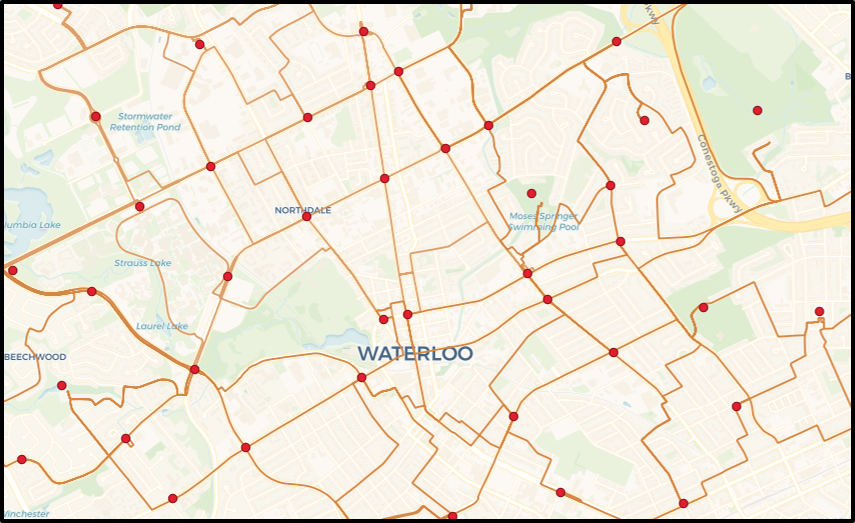
Figure 3: Example of the street network graph of the city of Waterloo used in the simulations. The figure shows a screenshot from the QGIS software. The shortest paths (orange lines) between vertices (red dots) are generated using the OpenRouteService.

To obtain the travel durations at each edge, we first sample robot speeds from a uniform random distribution. The travel durations under the two modes are then computed by dividing the edge length (computed using ORS) by the speed values and rounding off to the nearest integer. The travel speeds are sampled as follows: autonomous speed $u^{0}_{xy}\sim U[0,40]$; assisted speed $u^{1}_{xy}\sim U[10+u^{0}_{xy},30+u^{0}_{xy}]$. The maximum waiting duration at each vertex $x$ is sampled from a uniform random distribution as $\overline{w}_{x}\sim U[0,15]$. The operator availability function is generated by randomly sampling periods of availability and unavailability, with durations of each period sampled from the range of $[10,200]$. The distance values used in our simulations are in meters, times are in minutes and speeds are in meters/minute.

We test the algorithms using the Waterloo city map with varying vertex density, by selecting $64$, $100$ or $225$ vertices to be placed in the map. We generate $20$ problem instances for each density level (varying speeds, waiting limits and operator availability), and for each instance, we solve the problem for $100$ randomly selected pairs of start and goal vertices. The algorithms are compared based on solution time and the number of explored nodes. We also examine some of the solutions provided by the greedy method.

Note on implementation: All three graph search algorithms (Budget-$A^{*}$, Greedy and Time-expanded $A^{*}$) use the same heuristic, obtained by solving a problem instance under the assumption that operator is always available. This heuristic is admissible in a time-dependent graph [16] and can be computed efficiently. The priority queues used in all methods are implemented as binary heaps, allowing for efficient insertion, extraction and search operations. Additionally, all the methods require computation of the feasibility set (Alg. 2 line 5). This is pre-computed for all departure times and is given as input to each algorithm.

VI-C Results

Figure 4 compares the performance of the Budget-$A^{*}$ algorithm with that of the Greedy algorithm in terms of durations of the generated paths. From the figure, we observe that the Greedy algorithm is able to generate optimal or close-to-optimal solutions for a large proportion of the tested problem instances. However, for many instances, the path generated by the greedy approach is much longer than that produced by the Budget-$A^{*}$ algorithm, reaching up to twice the duration.

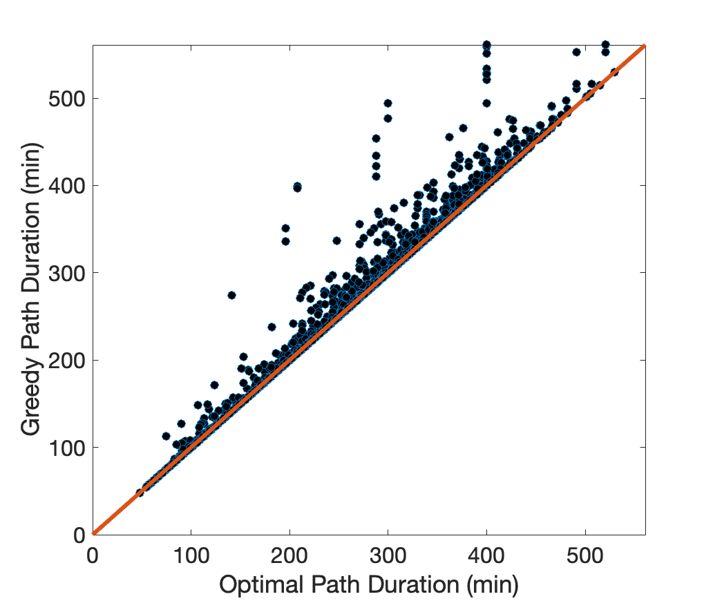
Figure 4: Performance comparison of the Greedy algorithm to the proposed Budget-$A^{*}$ algorithm. Each point in the graph denotes a problem instance, where the $x$ and $y$ coordinates correspond to durations of the paths generated by the Budget-$A^{*}$ and the Greedy algorithm respectively. The diagonal line represents equal path duration and the vertical distance from the line indicates the difference in duration between the two solutions.

To gain further insight into our results, we present Fig. 5, highlighting example instances where the greedy approach fails to generate an optimal solution. Through these examples, we demonstrate how our algorithm makes effective decisions regarding path selection, preemptive waiting, and not utilizing assistance to delay arrival at a later vertex. These decisions ultimately result in improved arrival time at the goal.

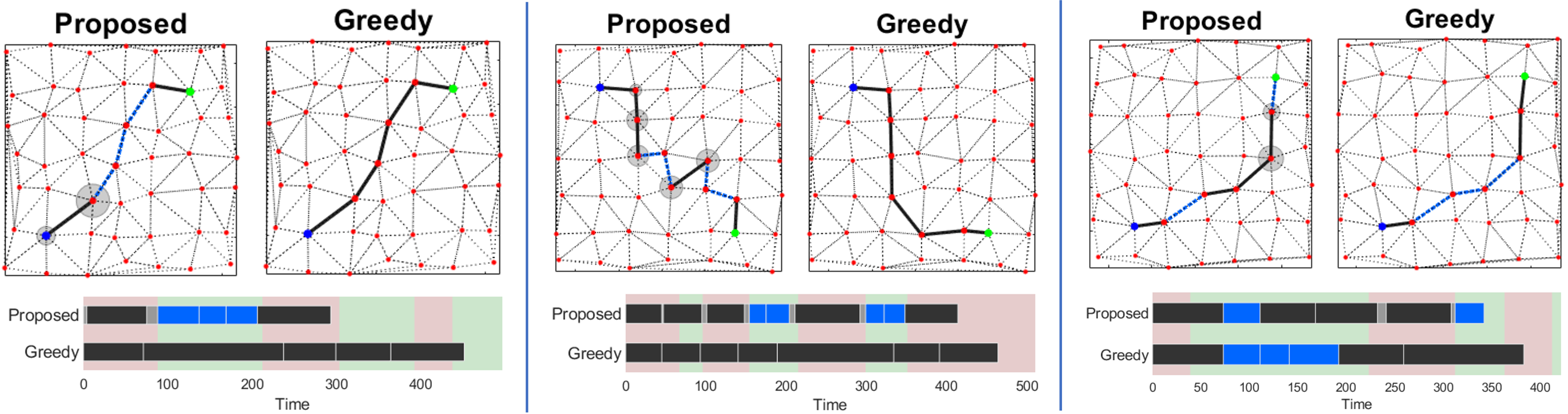
Figure 5: Example graphs comparing paths generated by the proposed Budget-$A^{*}$ and the Greedy algorithm. Black solid lines represent autonomous mode and blue dotted lines represent assisted mode. Grey circles denote waiting, with circle size proportional to waiting duration. The red and greed shaded regions in the bottom plots represent operator availability. (a) The Budget-$A^{*}$ algorithm preemptively waits at initial vertices to use autonomous mode for later edges, resulting in a faster path. The greedy algorithm moves towards the goal quickly, but cannot use operator availability later due to waiting limits. (b) The Budget-$A^{*}$ algorithm uses operator availability more efficiently by selecting a longer path. (c) The Budget-$A^{*}$ algorithm chooses not to use operator’s assistance even when it is available, so that it can be used later when the assistance is more beneficial.

Figure 6 compares the computation time required by different solution methods for varying number of vertices and the duration of the optimal path between the start and goal vertices. The plots demonstrate that the proposed algorithm consistently outperforms the other optimal methods in terms of computation time, with the greedy method being the fastest but providing suboptimal solutions. The computation time for all methods increases with the number of vertices. The path duration has the greatest impact on the performance of the TCSP-CWT algorithm, followed by the Time-expanded $A^{*}$, the Budget-$A^{*}$ algorithm, and finally the Greedy algorithm.

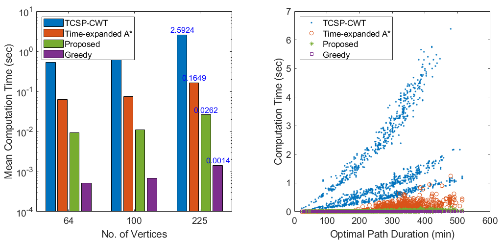
Figure 6: Computation time comparison for different methods. Left: Mean computation time as a function of the number of vertices in the graph, averaged over all test instances. Note that the time is plotted on a log scale. Right: Computation time as a function of actual duration of the optimal path, shown for all test instances.

Figure 7 compares the number of nodes generated and explored by Time-expanded $A^{*}$, Budget $A^{*}$, and Greedy search algorithms. The number of nodes is a key metric to evaluate search efficiency as it reflects the number of insertions and extractions from the priority queue. The Time-expanded $A^{*}$ generates nodes at a faster rate with increasing vertices, while the proposed algorithm generates an order of magnitude fewer nodes, indicating better efficiency and scalability. The Greedy search algorithm terminates after exploring the least number of nodes, indicating that it sacrifices optimality for speed. In contrast, both the Time-expanded $A^{*}$ and Budget $A^{*}$ algorithms guarantee optimality in their search results.

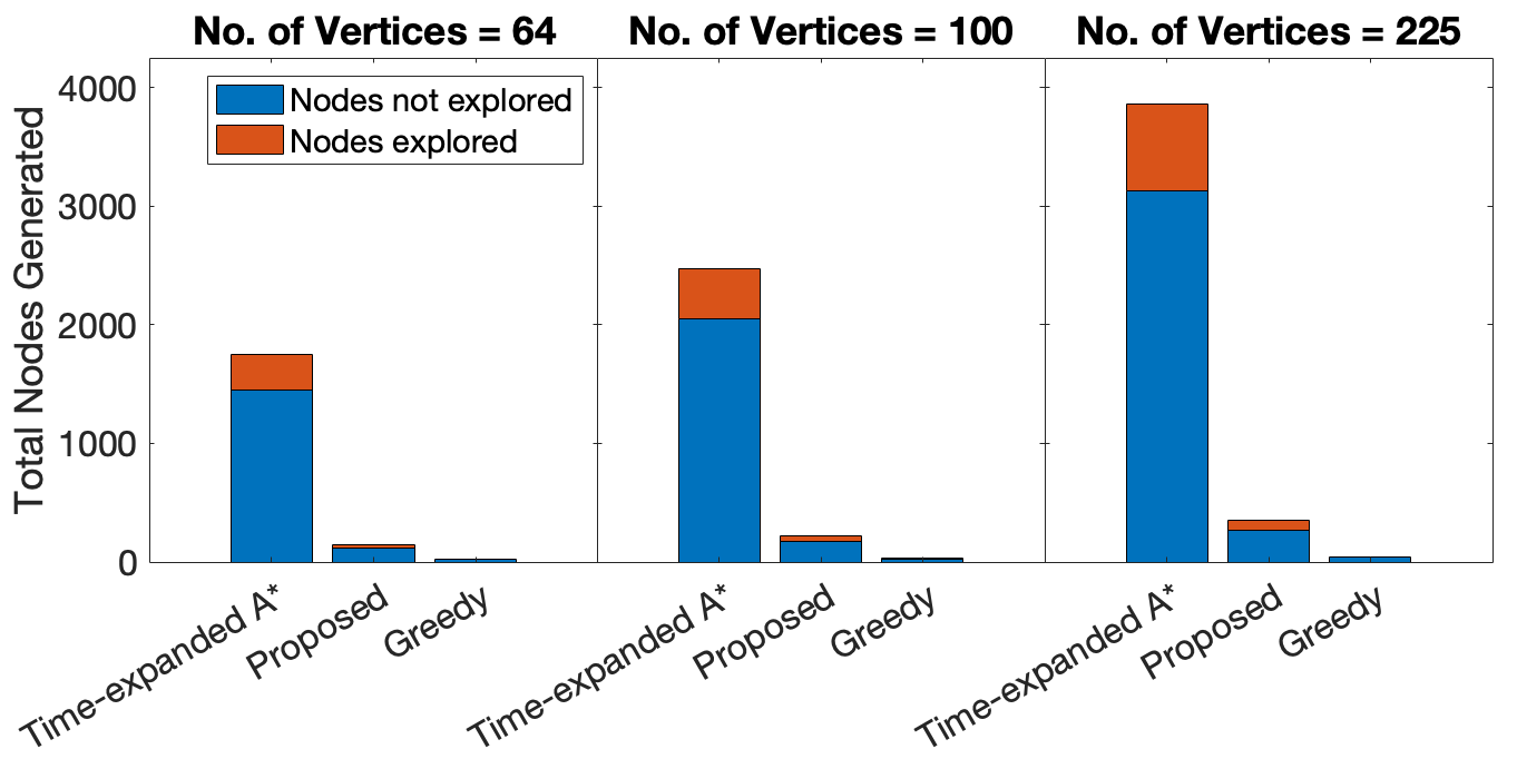
Figure 7: Mean number of nodes generated during graph search under the three methods for different number of vertices in the map. The bar height shows the total number of nodes generated and added to the queue during the search. The orange stack denotes the number of nodes explored before the goal is reached and the search is terminated.

VII Conclusion

In this paper, we introduced Budget-$A^{*}$, a new algorithm to tackle the problem of collaborative robot planning with bounded waiting constraints and intermittent human availability. Our approach computes the optimal execution path, which specifies which path should the robot take, how much to wait at each location and when to use human assistance. Our simulations on a city road network demonstrate that Budget-$A^{*}$ outperforms existing optimal methods, in terms of both computation time and number of nodes explored. Furthermore, we note that the greedy method performs well for the majority of test cases, which could potentially be utilized to further improve efficiency of the proposed algorithm.

For future research, the Budget-$A^{*}$ algorithm can be extended to handle more complex constraints such as multiple types of human assistance, non-stationary operator availability, and dynamic task requirements. Our approach can be further optimized to handle even larger networks by incorporating better heuristics and pruning techniques. Finally, our algorithm can be adapted to other applications such as emergency response in unknown environments, where fast and online task planning is crucial.

Our approach has significant implications for real-world applications like transportation systems, logistics, and scheduling, where time constraints and limited human supervision are crucial. We believe our work will inspire further research in these areas and lead to the development of more efficient algorithms for enabling human supervision under real-world restrictions.

References

- [1] L. Royakkers and R. van Est, “A literature review on new robotics: automation from love to war,” International journal of social robotics, vol. 7, pp. 549–570, 2015.
- [2] M. Mintrom, S. Sumartojo, D. Kulić, L. Tian, P. Carreno-Medrano, and A. Allen, “Robots in public spaces: Implications for policy design,” Policy Design and Practice, vol. 5, no. 2, pp. 123–139, 2022.
- [3] A. Dahiya, A. M. Aroyo, K. Dautenhahn, and S. L. Smith, “A survey of multi-agent human–robot interaction systems,” Robotics and Autonomous Systems, vol. 161, p. 104335, 2023.
- [4] D. G. Riley and E. W. Frew, “Assessment of coordinated heterogeneous exploration of complex environments,” in IEEE Conference on Control Technology and Applications (CCTA), 2021, pp. 138–143.
- [5] Y. Wang, Y. Yuan, Y. Ma, and G. Wang, “Time-dependent graphs: Definitions, applications, and algorithms,” Data Science and Engineering, vol. 4, pp. 352–366, 2019.
- [6] G. Swamy, S. Reddy, S. Levine, and A. D. Dragan, “Scaled autonomy: Enabling human operators to control robot fleets,” in IEEE International Conference on Robotics and Automation (ICRA), 2020, pp. 5942–5948.
- [7] A. Dahiya, N. Akbarzadeh, A. Mahajan, and S. L. Smith, “Scalable operator allocation for multirobot assistance: A restless bandit approach,” IEEE Transactions on Control of Network Systems, vol. 9, no. 3, pp. 1397–1408, 2022.
- [8] C. Hickert, S. Li, and C. Wu, “Cooperation for scalable supervision of autonomy in mixed traffic,” arXiv preprint arXiv:2112.07569, 2021.
- [9] Y. Cai, A. Dahiya, N. Wilde, and S. L. Smith, “Scheduling operator assistance for shared autonomy in multi-robot teams,” in IEEE Conference on Decision and Control (CDC), 2022, pp. 3997–4003.
- [10] F. Fusaro, E. Lamon, E. De Momi, and A. Ajoudani, “An integrated dynamic method for allocating roles and planning tasks for mixed human-robot teams,” in IEEE International Conference on Robot & Human Interactive Communication (RO-MAN), 2021, pp. 534–539.
- [11] S. K. K. Hari, A. Nayak, and S. Rathinam, “An approximation algorithm for a task allocation, sequencing and scheduling problem involving a human-robot team,” Robotics and Automation Letters, vol. 5, no. 2, pp. 2146–2153, 2020.
- [12] S. Mau and J. Dolan, “Scheduling for humans in multirobot supervisory control,” in 2007 IEEE/RSJ International Conference on Intelligent Robots and Systems. IEEE, 2007, pp. 1637–1643.
- [13] P. Gupta and V. Srivastava, “Optimal fidelity selection for human-in-the-loop queues using semi-markov decision processes,” in 2019 American Control Conference (ACC), 2019, pp. 5266–5271.
- [14] N. D. Powel and K. A. Morgansen, “Multiserver queueing for supervisory control of autonomous vehicles,” in 2012 American Control Conference (ACC). IEEE, 2012, pp. 3179–3185.
- [15] B. C. Dean, “Algorithms for minimum-cost paths in time-dependent networks with waiting policies,” Networks: An International Journal, vol. 44, no. 1, pp. 41–46, 2004.
- [16] L. Zhao, T. Ohshima, and H. Nagamochi, “A* algorithm for the time-dependent shortest path problem,” in WAAC08: The 11th Japan-Korea Joint Workshop on Algorithms and Computation, vol. 10, 2008.
- [17] A. Orda and R. Rom, “Shortest-path and minimum-delay algorithms in networks with time-dependent edge-length,” Journal of the ACM (JACM), vol. 37, no. 3, pp. 607–625, 1990.
- [18] B. Ding, J. X. Yu, and L. Qin, “Finding time-dependent shortest paths over large graphs,” in International Conference on Extending Database Technology: Advances in Database Technology, 2008, pp. 205–216.
- [19] M. Bentert, A.-S. Himmel, A. Nichterlein, and R. Niedermeier, “Efficient computation of optimal temporal walks under waiting-time constraints,” Applied Network Science, vol. 5, no. 1, pp. 1–26, 2020.
- [20] E. He, N. Boland, G. Nemhauser, and M. Savelsbergh, “Time-dependent shortest path problems with penalties and limits on waiting,” INFORMS Journal on Computing, vol. 33, no. 3, pp. 997–1014, 2021.
- [21] L. Foschini, J. Hershberger, and S. Suri, “On the complexity of time-dependent shortest paths,” in ACM-SIAM Symposium on Discrete Algorithms (SODA), 2011, pp. 327–341.
- [22] X. Cai, T. Kloks, and C.-K. Wong, “Time-varying shortest path problems with constraints,” Networks: An International Journal, vol. 29, no. 3, pp. 141–150, 1997.
- [23] L. R. Ford Jr and D. R. Fulkerson, “Constructing maximal dynamic flows from static flows,” Operations research, vol. 6, no. 3, pp. 419–433, 1958.