Peculiarities of beta functions in sigma models

Abstract

In this paper we consider perturbation theory in generic two-dimensional sigma models in the so-called first-order formalism, using the coordinate regularization approach. Our goal is to analyze the first-order formalism in application to $\beta$ functions and compare its results with the standard geometric calculations. Already in the second loop, we observe deviations from the geometric results that cannot be explained by the regularization/renormalization scheme choices. Moreover, in certain cases the first-order calculations produce results that are not symmetric under the classical diffeomorphisms of the target space. Although we could not present the full solution to this remarkable phenomenon, we found some indirect arguments indicating that an anomaly similar to that established in supersymmetric Yang-Mills theory might manifest itself starting from the second loop. We discuss why the difference between two answers might be an infrared effect, similar to that in $\beta$ functions in supersymmetric Yang-Mills theories.

In addition to the generic Kähler target spaces we discuss in detail the so-called Lie-algebraic sigma models. In particular, this is the case when the perturbed field $G^{i\bar{j}}$ is a product of the holomorphic and antiholomorphic currents satisfying two-dimensional current algebra.

1 Introduction

Sigma models on Kählerian and super-Kählerian target spaces play an important role in strings and various aspects of quantum field theory – from mathematics to phenomenology. If supersymmetrized in two dimensions, they have extendended supersymmetries, ${\mathcal{N}}=2$ or ${\mathcal{N}}=4$ . In generic Kählerian models with non-Einstein target space each order of perturbation theory brings in new geometric structures, (see e.g. Grah ; Foakes1987 ; Foakes1988 ; Ketov2000 ; Naka ), say, in the first- and second-loop orders we have

$${\mathcal{L}}_{\rm eff}=\left\{G_{i\bar{j}}+\left(\alpha^{\prime}R_{i\bar{j}}+\frac{(\alpha^{\prime})^{2}}{2}R_{i\bar{k}\ell\bar{m}}\,R_{\bar{j}}^{\,\,\bar{k}\ell\bar{m}}\right)L+...\right\}\partial_{\mu}\varphi^{i}\partial_{\mu}\bar{\varphi}^{\,\bar{j}}$$ (1)

where $L$ in Eq. (1) is defined as

$$L=-\log\frac{M_{\rm uv}}{\mu}\,.$$ (2)

Neither $R_{i\bar{j}}$ nor $R_{i\bar{k}\ell\bar{m}}\,R_{\bar{j}}^{\,\,\bar{k}\ell\bar{m}}$ reduce to $G_{i\bar{j}}$ in the general case.

In this paper, we first consider renormalization aspects of the so-called first order formalism in generic sigma models Losev2006 (for brevity referred to as the first-order sigma models). We treat these models as deformations of the conformal field theories of the simple bosonic “$\beta$-$\gamma$” systems by using the so-called coordinate approach to compute the beta function. We consider correlation functions in the real space (opposite to the traditional momentum) and employ the point-splitting regularization. This construction is a priori expected to produce beta functions of a certain self-repeating pattern of the (differential) polynomial type for the inverse metric $G^{i\bar{j}}$. Comparing with Eq. (1) we see that the expected pattern does emerge at one loop (see below). Although generalizing our analysis to higher loops we continue to observe the polynomial pattern, the $\beta$ function obtained in this way does not coincide with the result of the standard geometric calculation presented in (1) starting from the second loop Grah ; Foakes1987 ; Foakes1988 ; Tsey . Three-loop contribution is RG-scheme dependent – therefore one might blame the difference in the renormalization schemes for the disagreement.

However, the disagreement we observe appears already in the second loop. This leads us to the hypothesis that starting from the second loop a certain anomaly manifests itself, perhaps, similar to that established in supersymmetric Yang-Mills theory NSZV ; NSZV1 ; CS ; AH . Some indirect arguments in favor of this hypothesis will be given in Sec. 4.

Besides the generic Kähler target spaces we discuss in detail the so-called Lie-algebraic sigma models. In paricular, this is the case when the perturbed field $G^{i\bar{j}}$ is a product of the holomorphic and antiholomorphic currents satisfying two-dimensional current algebra. We obtain exact formulas for the one and two-loop beta functions using only algebraic data and observe the full correspondence with the known results for current-current deformations of the conformal field theories Kutasov1989 ; PhysRevLett.86.4753 ; Ludwig2003 (but not with the geometric formulas).

The paper is organized as follows. In Sec. (2) we introduce first-order sigma model, outline the two-loop computation of the $\beta$ function and discuss why the answer is different from the one in Eq. (1). In Sec. (3) we discuss an important example of the current-current perturbation, which we also dub as Lie-algebraic sigma models, and show why the answer in Sec. (2) makes sense from the algebraic point of view. In Sec. (4) we indicate that discrepancies between the“geometric” and “algebraic” $\beta$ functions can be an IR effect. Illuminating instanton calculations are presented in Sec. (5).

2 Coordinate $\beta$ function

2.1 Model and derivation

The first order sigma model proposed in Losev2006 and further developed in Zeitlin2006 ; Zeitlin2008 ; Zeitlin2009 , was initially introduced as a tool to address singular background in string theory. More specifically, the bare action is described by the following conformal field theory

$$S_{0}=\frac{1}{\alpha^{\prime}}\int\frac{d^{2}z}{\pi}\left(p_{a}\bar{\partial}\varphi^{a}+\bar{p}_{\bar{a}}\partial\bar{\varphi}^{\bar{a}}\right).$$ (3)

Here $d^{2}z=dxdy=idz\wedge d\bar{z}/2$, the index $a$ runs from $1$ to $D/2$ (here we have assumed that the target space is a complex manifold with local coordinates $\varphi^{a}$ and $\bar{\varphi}^{\bar{a}}$). The fields $p_{a}$, $p_{\bar{a}}$ are $(1,0)$ and $(0,1)$ forms on $\Sigma$ correspondingly, and the fields $\varphi^{a}$, $\varphi^{\bar{a}}$ are scalars. For our purposes, it will be enough to consider $\Sigma=\mathds{C}P^{1}$. For more precise definitions and discussion about the choice of complex structure see nekrasov2005lectures . To simplify notations in what follows we put $\alpha^{\prime}=1$.

The action (3) is equivalent to the following operator product expansions,

$$p_{a}(z)\varphi^{b}(w)=\frac{\delta_{a}^{b}}{z-w}+{\rm reg},\qquad\bar{p}_{\bar{a}}(\bar{z})\bar{\varphi}^{\bar{b}}(\bar{w})=\frac{\delta_{\bar{a}}^{\bar{b}}}{\bar{z}-\bar{w}}+{\rm reg}.$$ (4)

To turn to the non-singular sigma models one considers perturbation of the action (3) by four possible classically marginal terms

$$S=S_{0}-\int\frac{d^{2}z}{\pi}(O_{G}+O_{\mu}+O_{\bar{\mu}}+O_{b})$$ (5)

where

$$O_{G}=G^{a\bar{a}}p_{a}\bar{p}_{\bar{a}},\qquad O_{\mu}=p_{a}\mu^{a}_{\bar{a}}\bar{\partial}\bar{\varphi}^{\bar{a}},\qquad O_{\bar{\mu}}=\bar{p}_{\bar{a}}\bar{\mu}_{a}^{\bar{a}}\partial\varphi^{a},\qquad O_{b}=b_{a\bar{a}}\partial\varphi^{a}\bar{\partial}\bar{\varphi}^{\bar{a}}.$$ (6)

Assuming that $G^{a\bar{a}}$ is not degenerate one can integrate over $p$ and $\bar{p}$ and obtain the second-order sigma model with the metric and Kalb-Ramond fields parametrized in terms of the data $G$, $b$, $\mu$ and $\bar{\mu}$ (see Losev2006 ). Besides, an additional field of a dilaton appears due to the anomaly in the path integral measure.

For operators (6) to be primary, in the first order of perturbation theory one has to impose transversality condition

$$\partial_{a}G^{a\bar{a}}=\partial_{\bar{a}}G^{a\bar{a}}=\partial_{a}\mu^{a}_{\bar{a}}=\partial_{\bar{a}}\bar{\mu}_{a}^{\bar{a}}=0.$$ (7)

This in particular allows one to avoid possible self-contractions of $p$ and $\varphi$ inside operators. In what follows, we will not insist on the transversality condition and presume that self-contractions are subtracted, in other words the operators are normal-ordered.

In this paper we focus mainly on the case when only $O_{G}$ perturbations are present – then the metric and Kalb-Ramond fields are, respectively, symmetric and antisymmetric forms of inverse of the bivector $G^{a\bar{a}}$, which we denote by $G_{a\bar{a}}$. The dilaton field $\Phi$ is proportional to the logarithm of the determinant

$$\Phi\sim\log\det G\,.$$

Note that for Kählerian metrics with constant determinant the effects due to the Kalb-Ramond fields and dilatons are irrelevant.

Here again, we stress that the first order system makes sense even when the inverse of $G^{a\bar{a}}$ does not exist. Our point of view is that the original sigma model is represented by Lagrangian (5). In this paper we focus on making sense of (5) as a quantum field theory.

First, let us focus on the case when $b_{a\bar{a}}=\bar{\mu}_{a}^{\bar{a}}=\mu^{a}_{\bar{a}}=0$, i.e. on the action

$$S=\int\frac{d^{2}z}{\pi}\left(p_{a}\bar{\partial}\varphi^{a}+\bar{p}_{\bar{a}}\partial\bar{\varphi}^{\bar{a}}-G^{a\bar{a}}(\varphi,\bar{\varphi})p_{a}\bar{p}_{\bar{a}}\right).$$ (8)

We can regard $G$ as a perturbation for the conformal field theory given by $S_{0}$ in Eq. (3). Let us demonstrate the necessity of renormalization using the example of the perturbative calculation of the following two-point function,

$$C_{2}(x,y)=\Big{\langle}B(x)O_{g}(y)\Big{\rangle}_{G}\equiv\Big{\langle}B(x)O_{g}(y)\exp\left(\int_{|z|<R}\frac{d^{2}z}{\pi}O_{G}\right)\Big{\rangle}_{0}.$$ (9)

Here

$$B(x)\equiv b_{c\bar{c}}\partial\varphi^{c}\bar{\partial}\bar{\varphi}^{\bar{c}}$$

is a composite field which is denoted differently from $O_{b}$ to emphasize the fact that the field $b_{a\bar{a}}$ is an observable (and not the one in the action). By $O_{g}$ we denote $g^{a\bar{a}}p_{a}\bar{p}_{\bar{a}}$ again to emphasize different role of the observable field $g^{a\bar{a}}$ as opposed to to $G^{a\bar{a}}$ in the exponential. All observables are considered to be normal ordered, so we don’t have to worry about self-contractions. The effect of non-zero $G$ is included order by order in the perturbation theory which is symbolized by the last equality in (9). The subscript there reflects that computations are carried out in the free theory (3). Here we have also introduced an IR cut-off $R$ and assume that $|x|\ll R$, $y\ll R$. In the zeroth order using OPE (4) we conclude

$$C_{2}^{(0)}(x,y)=\frac{g^{a\bar{a}}b_{a\bar{a}}}{|x-y|^{4}}.$$ (10)

At this point, we have to clarify what we mean by correlation functions as functions of the target space fields. Strictly speaking instead of $g^{a\bar{a}}b_{a\bar{a}}$ one has to consider an integral

$$\int\,g^{a\bar{a}}(\varphi^{(0)})b_{a\bar{a}}(\varphi^{(0)})\,d^{D}\varphi^{(0)}$$ (11)

over the modes $\varphi^{(0)}$ of the $\varphi$-fields. We assume that the target space is compact, or that the observables $g^{a\bar{a}}$, $b_{a\bar{a}}$ are functions rapidly vanishing at the “space-time infinity,” so that all integrals are convergent.

We assume this prescription for all the correlation functions in this paper.

In particular, this will allow us to integrate by parts in some of the examples below. Note also that we use Wick’s theorem to contract derivatives of the field, which would, otherwise, vanish after the integration.

The next order is given by an integral of the three-point function

$$C_{2}^{(1)}(x,y)=\int\limits_{|z|<R}\frac{d^{2}z}{\pi}\Big{\langle}B(x)O_{g}(y)O_{G}(z)\Big{\rangle}_{0}.$$ (12)

In this case the computation of the correlation function is a bit more complicated, but still can be performed explicitly. Namely, after contracting the $p$ field with the derivatives we arrive at

$$\Big{\langle}B(x)O_{g}(y)O_{G}(z)\Big{\rangle}_{0}=\frac{\langle b_{a\bar{a}}(x)g^{a\bar{a}}(y)G^{c\bar{c}}p_{c}\bar{p}_{\bar{c}}(z)\rangle}{|x-y|^{4}}+\frac{\langle b_{a\bar{a}}(x)g^{a\bar{b}}\bar{p}_{\bar{b}}(y)G^{c\bar{a}}p_{c}(z)\rangle}{(x-y)^{2}(\bar{x}-\bar{z})^{2}}+\left(\begin{array}[]{c}y\leftrightarrow z\\ G\leftrightarrow g\end{array}\right).$$ (13)

Contracting the remaining $p$ field we obtain

$$\frac{\langle b_{a\bar{a}}(x)g^{a\bar{a}}(y)G^{c\bar{c}}p_{c}\bar{p}_{\bar{c}}(z)\rangle}{|x-y|^{4}}=\frac{G^{c\bar{c}}\partial_{c}\partial_{\bar{c}}b_{a\bar{a}}(x)g^{a\bar{a}}(y)}{|x-y|^{4}|z-x|^{2}}+\frac{G^{c\bar{c}}\partial_{c}b_{a\bar{a}}(x)\partial_{\bar{c}}g^{a\bar{a}}(y)}{|x-y|^{4}(z-x)(\bar{z}-\bar{y})}+\left(\begin{array}[]{c}y\leftrightarrow x\\ g\leftrightarrow b\end{array}\right),$$ (14)

$$\langle b_{a\bar{a}}(x)g^{a\bar{b}}\bar{p}_{\bar{b}}(y)G^{c\bar{a}}p_{c}(z)\rangle=\frac{\partial_{\bar{b}}\partial_{c}b_{a\bar{a}}g^{a\bar{b}}G^{c\bar{a}}}{(\bar{y}-\bar{x})(z-x)}+\frac{\partial_{\bar{b}}b_{a\bar{a}}\partial_{c}g^{a\bar{b}}G^{c\bar{a}}}{(\bar{y}-\bar{x})(z-y)}+\frac{b_{a\bar{a}}\partial_{c}g^{a\bar{b}}\partial_{\bar{b}}G^{c\bar{a}}}{(\bar{y}-\bar{z})(z-y)}+\frac{\partial_{c}b_{a\bar{a}}g^{a\bar{b}}\partial_{\bar{b}}G^{c\bar{a}}}{(\bar{y}-\bar{z})(z-x)}$$ (15)

Assembling everything together we obtain an expression for the correlator that does not look like a typical three point function in CFT. This happened because we relaxed the transversality condition, which on this level is equivalent to the statement that operators are primary. Anyhow, from the obtained expression one might expect possible divergences when the integration comes close to $x$ or $y$, therefore we add UV regularization prescription that small disks of the size $\epsilon$ are excluded from the integration domain, namely $|z-x|<\epsilon$, $|z-y|<\epsilon$. Performing integration with such a prescription we obtain

$$C_{2}^{(1)}(x,y)=\frac{\log\frac{|x-y|^{2}}{\epsilon^{2}}}{|x-y|^{4}}\Big{(}g^{a\bar{a}}\bm{[}b,G\bm{]}_{a\bar{a}}+b_{a\bar{a}}\bm{[}g,G\bm{]}^{a\bar{a}}\Big{)}+\delta C_{2}^{(1)}(x,y)$$ (16)

where $\delta C_{2}^{(1)}$ is present only due to effects of the fields being non-primary (non-tranversal in the sense of Eq. (7)),

$$\delta C_{2}^{(1)}(x,y)=\frac{G^{c\bar{c}}\partial_{c}\partial_{\bar{c}}(b_{a\bar{a}}g^{a\bar{a}})}{|x-y|^{4}}\log\frac{R^{2}}{|x-y|^{2}}+\frac{4}{\epsilon^{2}}\frac{g^{c\bar{c}}\partial_{c}\partial_{\bar{c}}(b_{a\bar{a}}G^{a\bar{a}})}{|x-y|^{2}}\\ +\frac{\partial_{c}(b_{a\bar{a}}G^{a\bar{c}})\partial_{\bar{c}}g^{c\bar{a}}+\partial_{c}g^{a\bar{c}}\partial_{\bar{c}}(b_{a\bar{a}}G^{c\bar{a}})-g^{c\bar{c}}\partial_{\bar{c}}(b_{a\bar{a}}\partial_{c}G^{a\bar{a}})-g^{c\bar{c}}\partial_{c}(b_{a\bar{a}}\partial_{\bar{c}}G^{a\bar{a}})}{|x-y|^{4}}.$$ (17)

Notice that if trasversality condition (7) is satisfied then $\delta C_{2}^{(1)}$ vanishes after integration by parts in the target space (see Eq. (11)).

The coordinate part of the first term in Eq. (16) is universal for the correlation functions in deformed CFT Cardy:1989da ; Ginsparg:1988ui ; Zamolodchikov:1989we , while the field dependent coefficient represents the OPE data. The expression in the bold squared parentheses in (16) are bilinear operations, which are explicitly given by

$$\bm{[}b,G\bm{]}_{a\bar{a}}=\partial_{\bar{c}}b_{c\bar{a}}\partial_{a}G^{c\bar{c}}+b_{c\bar{c}}\partial_{a}\partial_{\bar{a}}G^{c\bar{c}}+G^{c\bar{c}}\partial_{c}\partial_{\bar{c}}b_{a\bar{a}}+\partial_{c}b_{a\bar{c}}\partial_{\bar{a}}G^{c\bar{c}}$$ (18)

$$\bm{[}g,G\bm{]}^{a\bar{a}}=g^{c\bar{c}}\partial_{c}\partial_{\bar{c}}G^{a\bar{a}}-\partial_{\bar{c}}g^{c\bar{a}}\partial_{c}G^{a\bar{c}}+(G\leftrightarrow g).$$ (19)

In (18), (19) and in what follows the brackets $\bm{[\,\,]}$ typeset in bold acting on two tensors are to be understood as a tensor product of the Lie derivatives acting in holomorphic and antiholomorphic sectors. They also have a close relation to the Courant/Dorfman brackets Zeitlin2008 .

Therefore, to remove UV divergences we can perform the following renormalization,

$$B\to B^{(1)}=\left(b_{a\bar{a}}-\bm{[}b,G\bm{]}_{a\bar{a}}\log\frac{\rho^{2}}{\epsilon^{2}}\right)\partial\varphi^{a}\bar{\partial}\bar{\varphi}^{\bar{a}}-\frac{4}{\epsilon^{2}}b_{a\bar{a}}G^{a\bar{a}},$$ (20)

$$O_{g}\to O^{(1)}_{g}=\left(g^{a\bar{a}}-\bm{[}g,G\bm{]}^{a\bar{a}}\log\frac{\rho^{2}}{\epsilon^{2}}\right)p_{a}\bar{p}_{\bar{a}}.$$ (21)

Here the logarithm plays the same role as in Eqs. (1), (2) upon the replacement of the momentum cutoff by the coordinate regulator $M_{uv}\to\epsilon^{-1}$ and the renormalization point $\mu\to\rho^{-1}$. In this way, the renormalized correlation function reduces to

$$\langle B^{(1)}(x)O^{(1)}_{g}(y)\rangle=\frac{\log\frac{|x-y|^{2}}{\rho^{2}}}{|x-y|^{4}}\left(g^{a\bar{a}}\bm{[}b,G\bm{]}_{a\bar{a}}+b_{a\bar{a}}\bm{[}g,G\bm{]}^{a\bar{a}}\right)+\frac{G^{c\bar{c}}\partial_{c}\partial_{\bar{c}}(b_{a\bar{a}}g^{a\bar{a}})}{|x-y|^{4}}\log\frac{R^{2}}{|x-y|^{2}}\\[5.69054pt] +\frac{\partial_{c}(b_{a\bar{a}}G^{a\bar{c}})\partial_{\bar{c}}g^{c\bar{a}}+\partial_{c}g^{a\bar{c}}\partial_{\bar{c}}(b_{a\bar{a}}G^{c\bar{a}})-g^{c\bar{c}}\partial_{\bar{c}}(b_{a\bar{a}}\partial_{c}G^{a\bar{a}})-g^{c\bar{c}}\partial_{c}(b_{a\bar{a}}\partial_{\bar{c}}G^{a\bar{a}})}{|x-y|^{4}}+O(G^{2}).$$ (22)

Proceeding in the same way step by step one can derive renormalization in the higher orders. Unfortunately, all expressions become more and more bulky; besides, as we see, a lot of other terms are produced that are not responsible for the renormalization. To avoid at least part of these problems we change our approach a bit.

Namely, since we are mostly interested in the renormalization of $O_{g}$, we limit integration to $|z|<R$ and assume that $|y|<R$ but $|x|\gg R$. In this sense the perturbation does not “touch” observable $B(x)$. Then in the leading order we immediately obtain the $O_{g}$ renormalization directly

$$\int\limits_{|z|<R}\frac{d^{2}z}{\pi}\Big{\langle}B(x)O_{g}(0)O_{G}(z)\Big{\rangle}_{0}=\frac{b_{a\bar{a}}\bm{[}g,G\bm{]}^{a\bar{a}}}{|x|^{4}}\int\limits_{|z|<R}\frac{d^{2}z}{\pi}\frac{1}{|z|^{2}}=\frac{b_{a\bar{a}}\bm{[}g,G\bm{]}^{a\bar{a}}}{|x|^{4}}\log\frac{R^{2}}{\epsilon^{2}}$$ (23)

Here we have put coordinate of $O_{g}$ to zero $y=0$ because in the leading order of $|x|\to\infty$ the rest of the correlation function retains transnational invariance. In the next order we have to compute

$$C_{2}^{(2)}(x)=\frac{1}{2}\int\limits_{\Sigma_{\epsilon}}\frac{d^{2}z_{1}}{\pi}\frac{d^{2}z_{2}}{\pi}\Big{\langle}B(x)O_{g}(0)O_{G}(z_{1})O_{G}(z_{2})\Big{\rangle}_{0}$$ (24)

The integration domain $\Sigma_{\epsilon}$ is defined as

$$\epsilon\leq|z_{1}|\leq R,\qquad\epsilon\leq|z_{2}|\leq R,\qquad\epsilon\leq|z_{1}-z_{2}|\leq R.$$ (25)

Note extra IR regularization $|z_{1}-z_{2}|\leq R$; it does not affect the UV divergences but significantly simplifies computations as it makes $\Sigma_{\epsilon}$ invariant under various changes of variables , for example, $z_{1}\leftrightarrow z_{2}$; $z_{1}\to\bar{z}_{1}$, $z_{2}\to\bar{z_{2}}$; $z_{1}\to z_{2}-z_{1}$, $z_{2}\to z_{2}$ etc. Using this invariance and routinely contracting $p$ and $\varphi$ using OPE (4) and the Wick’s theorem we observe that only four possible structures appears in $C_{2}^{(2)}(x)$

$$C_{2}^{(2)}(x)=\frac{1}{|x|^{4}}\sum\limits_{i=1}^{4}\mathcal{A}_{i}I_{i}$$ (26)

with

$$I_{1}=\int\limits_{\Sigma_{\epsilon}}\frac{d^{2}z_{1}}{\pi}\frac{d^{2}z_{2}}{\pi}\frac{1}{|z_{1}|^{2}|z_{2}|^{2}},\qquad I_{2}=\int\limits_{\Sigma_{\epsilon}}\frac{d^{2}z_{1}}{\pi}\frac{d^{2}z_{2}}{\pi}\frac{1}{z_{2}^{2}\bar{z}_{1}(\bar{z}_{2}-\bar{z}_{1})}$$ (27)

$$I_{3}=\int\limits_{\Sigma_{\epsilon}}\frac{d^{2}z_{1}}{\pi}\frac{d^{2}z_{2}}{\pi}\frac{1}{z_{1}^{2}\bar{z}_{2}^{2}},\qquad I_{4}=\int\limits_{\Sigma_{\epsilon}}\frac{d^{2}z_{1}}{\pi}\frac{d^{2}z_{2}}{\pi}\frac{1}{|z_{1}|^{4}}.$$ (28)

In the appendix (A) we demonstrate that the integrals can be expressed as

$$I_{1}=L_{\epsilon}^{2},\qquad I_{2}=L_{\epsilon},\qquad I_{3}=0,\qquad I_{4}=R^{2}/\epsilon^{2}.$$ (29)

Here

$$L_{\epsilon}\equiv\log R^{2}/\epsilon^{2}\,.$$

The corresponding tensor structures $\mathcal{A}_{i}$ read as

$$\mathcal{A}_{1}=\frac{b_{a\bar{a}}\bm{[}g,\bm{[}G,G\bm{]}\bm{]}^{a\bar{a}}}{4}+\frac{b_{a\bar{a}}\bm{[}\bm{[}g,G\bm{]},G\bm{]}^{a\bar{a}}}{2},\qquad\mathcal{A}_{2}=\frac{1}{2}b_{a\bar{a}}\bm{[}g,G,G\bm{]}^{a\bar{a}}$$ (30)

$$\mathcal{A}_{3}=b_{a\bar{a}}(\partial_{c}G^{k\bar{a}}\partial_{k}\partial_{\bar{k}}G^{c\bar{c}}\partial_{\bar{c}}g^{a\bar{k}}+\partial_{c}g^{k\bar{a}}\partial_{k}\partial_{\bar{k}}G^{c\bar{c}}\partial_{\bar{c}}G^{a\bar{k}}),$$ (31)

$$\mathcal{A}_{4}=\frac{b_{a\bar{a}}}{2}(g^{a\bar{a}}\partial_{k}\partial_{\bar{k}}G^{c\bar{c}}\partial_{c}\partial_{\bar{c}}G^{k\bar{k}}+2G^{a\bar{a}}\partial_{k}\partial_{\bar{k}}G^{c\bar{c}}\partial_{c}\partial_{\bar{c}}g^{k\bar{k}})$$ (32)

where quadratic brackets are the operations defined as above (18), (19) that the qubic bracket is given by

$$\bm{[}g,G,G\bm{]}^{a\bar{a}}=\partial_{\bar{k}}G^{c\bar{c}}\partial_{\bar{c}}G^{k\bar{k}}\partial_{c}\partial_{k}g^{a\bar{a}}+\partial_{k}G^{c\bar{c}}\partial_{c}G^{k\bar{k}}\partial_{\bar{c}}\partial_{\bar{k}}g^{a\bar{a}}+2\partial_{k}G^{c\bar{c}}\partial_{c}g^{k\bar{k}}\partial_{\bar{k}}\partial_{\bar{c}}G^{a\bar{a}}+\\[5.69054pt] 2\partial_{\bar{k}}G^{c\bar{c}}\partial_{\bar{c}}g^{k\bar{k}}\partial_{k}\partial_{c}G^{a\bar{a}}+\partial_{c}\partial_{\bar{c}}G^{k\bar{k}}(\partial_{k}g^{c\bar{c}}\partial_{\bar{k}}G^{a\bar{a}}+\partial_{\bar{k}}g^{c\bar{c}}\partial_{k}G^{a\bar{a}}+\partial_{k}g^{a\bar{a}}\partial_{\bar{k}}G^{c\bar{c}}+\\[5.69054pt] \partial_{\bar{k}}g^{a\bar{a}}\partial_{k}G^{c\bar{c}}+g^{a\bar{c}}\partial_{k}\partial_{\bar{k}}G^{c\bar{a}}+G^{a\bar{c}}\partial_{k}\partial_{\bar{k}}g^{c\bar{a}}+g^{c\bar{a}}\partial_{k}\partial_{\bar{k}}G^{a\bar{c}}+G^{c\bar{a}}\partial_{k}\partial_{\bar{k}}g^{a\bar{c}})\\[5.69054pt] +\partial_{c}\partial_{\bar{c}}g^{k\bar{k}}(\partial_{k}G^{c\bar{c}}\partial_{\bar{k}}G^{a\bar{a}}+\partial_{\bar{k}}G^{c\bar{c}}\partial_{k}G^{a\bar{a}}+G^{c\bar{a}}\partial_{k}\partial_{\bar{k}}G^{a\bar{c}}+G^{a\bar{c}}\partial_{k}\partial_{\bar{k}}G^{c\bar{a}})\\[5.69054pt] -(g^{k\bar{a}}\partial_{\bar{k}}G^{c\bar{c}}+G^{k\bar{a}}\partial_{\bar{k}}g^{c\bar{c}})\partial_{k}\partial_{c}\partial_{\bar{c}}G^{a\bar{k}}-(g^{a\bar{k}}\partial_{k}G^{c\bar{c}}+G^{a\bar{k}}\partial_{k}g^{c\bar{c}})\partial_{\bar{k}}\partial_{c}\partial_{\bar{c}}G^{k\bar{a}}\\[5.69054pt] -2\partial_{k}\partial_{\bar{c}}G^{a\bar{k}}(\partial_{\bar{k}}g^{c\bar{c}}\partial_{c}G^{k\bar{a}}+\partial_{\bar{k}}G^{c\bar{c}}\partial_{c}g^{k\bar{a}})-2\partial_{c}\partial_{\bar{k}}G^{k\bar{a}}(\partial_{k}g^{c\bar{c}}\partial_{\bar{c}}G^{a\bar{k}}+\partial_{k}G^{c\bar{c}}\partial_{\bar{c}}g^{a\bar{k}})\\[5.69054pt] -G^{k\bar{a}}\partial_{\bar{k}}G^{c\bar{c}}\partial_{k}\partial_{c}\partial_{\bar{c}}g^{a\bar{k}}-G^{a\bar{k}}\partial_{k}G^{c\bar{c}}\partial_{\bar{k}}\partial_{c}\partial_{\bar{c}}g^{k\bar{a}}\\[5.69054pt] -2\partial_{\bar{k}}G^{c\bar{c}}\partial_{c}G^{k\bar{a}}\partial_{k}\partial_{\bar{c}}g^{a\bar{k}}-2\partial_{\bar{c}}G^{a\bar{k}}\partial_{k}G^{c\bar{c}}\partial_{c}\partial_{\bar{k}}g^{k\bar{a}}.$$ (33)

Now we have to deform $O_{g}$ and $O_{G}$ by addition of some counterterms to make the correlation function finite when $\epsilon\to 0$. In particular, to remove contribution from $\mathcal{A}_{4}$ we have to shift $O_{g}$ by the scalar observable

$$O_{g}\to O_{g}-\frac{\partial_{k}\partial_{\bar{k}}G^{c\bar{c}}\partial_{c}\partial_{\bar{c}}g^{k\bar{k}}}{\epsilon^{2}}.$$ (34)

Note that the first term in $\mathcal{A}_{4}$ has a disconnected character and disappears after taking into account contributions from the partition function. The remaining part of the correlation function reads.

$$C_{2}^{(1)}(x)+C_{2}^{(2)}(x)=\frac{b_{a\bar{a}}}{|x|^{4}}\left(g^{a\bar{a}}+L_{\epsilon}\bm{[}g,G\bm{]}^{a\bar{a}}+\frac{L_{\epsilon}^{2}}{4}\bm{[}g,\bm{[}G,G\bm{]}\bm{]}^{a\bar{a}}\right.\\ \left.+\frac{L_{\epsilon}^{2}}{2}\bm{[}\bm{[}g,G\bm{]},G\bm{]}^{a\bar{a}}+\frac{L_{\epsilon}\bm{[}g,G,G\bm{]}^{a\bar{a}}}{2}\right)$$ (35)

To understand renormalization further we have to separate deformation of $O_{g}$ and $O_{G}$. In typical Callan-Symanzik approach that would correspond to $\beta$ and $\gamma$ functions zJJ . For this we consider the following one-point function,

$$C_{1}(x)=\Big{\langle}B(x)\exp\left(\int_{|z|<R}\frac{d^{2}z}{\pi}G^{a\bar{a}}(\varphi,\bar{\varphi})p_{a}\bar{p}_{\bar{a}}\right)\Big{\rangle}_{0}$$ (36)

Again here it is assumed that $|x|\gg R$. Its expansion up to the fourth order in $G^{a\bar{a}}$ can be deduced from (35)

$$|x|^{4}C_{1}(x)=b_{a\bar{a}}\left(G+\frac{L_{\epsilon}}{2}\bm{[}G,G\bm{]}+\frac{L_{\epsilon}^{2}}{4}\bm{[}G,\bm{[}G,G\bm{]}\bm{]}+\frac{L_{\epsilon}}{3!}\bm{[}G,G,G\bm{]}\right)^{a\bar{a}}$$ (37)

To make it finite as $\epsilon\to 0$ we have to deform $G$ in the following way

$$G\to\tilde{G}=G-\frac{\bm{[}G,G\bm{]}}{2}\ell+\frac{(\ell)^{2}}{4}\bm{[}G,\bm{[}G,G\bm{]}\bm{]}-\frac{\ell}{3!}\bm{[}G,G,G\bm{]}+O(G^{4})$$ (38)

with

$$\ell=\log\frac{\rho^{2}}{\epsilon^{2}}\,.$$

Then

$$\tilde{G}+\frac{L_{\epsilon}}{2}\bm{[}\tilde{G},\tilde{G}\bm{]}+\frac{L_{\epsilon}^{2}}{4}\bm{[}\tilde{G},\bm{[}\tilde{G},\tilde{G}\bm{]}\bm{]}+\frac{L_{\epsilon}}{3!}\bm{[}\tilde{G},\tilde{G},\tilde{G}\bm{]}=\\ G-\frac{\bm{[}G,G\bm{]}}{2}L_{\rho}+\frac{(L_{\rho})^{2}}{4}\bm{[}G,\bm{[}G,G\bm{]}\bm{]}-\frac{L_{\rho}}{3!}\bm{[}G,G,G\bm{]}+O(G^{4}),$$ (39)

where now

$$L_{\rho}=\log R^{2}/\rho^{2}\,.$$

Now we can study the flow of the deformed observable

$$\frac{\partial\tilde{G}}{\partial\ell}=-\frac{\bm{[}G,G\bm{]}}{2}+\frac{\ell}{2}\bm{[}G,\bm{[}G,G\bm{]}\bm{]}-\frac{1}{3!}\bm{[}G,G,G\bm{]}+O(G^{4})=-\frac{\bm{[}\tilde{G},\tilde{G}\bm{]}}{2}-\frac{\bm{[}\tilde{G},\tilde{G},\tilde{G}\bm{]}}{3!}+O(\tilde{G}^{4})$$ (40)

We see that contrary to the deformation (38) the flow (40) does not contain logarithms but only the observables. Following the traditional notation we call this flow a beta function

$$-\frac{\partial\tilde{G}}{\partial\ell}=\beta_{2}(\tilde{G})+\beta_{3}(\tilde{G})+O(\tilde{G}^{4})$$ (41)

with

$$\boxed{\beta_{2}^{a\bar{a}}(G)=\frac{\bm{[}G,G\bm{]}^{a\bar{a}}}{2}=G^{c\bar{c}}\partial_{c}\partial_{\bar{c}}G^{a\bar{a}}-\partial_{c}G^{a\bar{c}}\partial_{\bar{c}}G^{c\bar{a}}}$$ (42)

$$\beta_{3}^{a\bar{a}} =\frac{\bm{[}G,G,G\bm{]}^{a\bar{a}}}{3!}=\frac{1}{2}\left(\partial_{\bar{k}}G^{c\bar{c}}\partial_{c}(\partial_{k}G^{a\bar{a}}\partial_{\bar{c}}G^{k\bar{k}}-G^{k\bar{a}}\partial_{k}\partial_{\bar{c}}G^{a\bar{k}})\right.$$

$$+ \partial_{k}G^{c\bar{c}}\partial_{\bar{c}}(\partial_{\bar{k}}G^{a\bar{a}}\partial_{c}G^{k\bar{k}}-G^{a\bar{k}}\partial_{c}\partial_{\bar{k}}G^{k\bar{a}})+$$

$$\left.\partial_{k}\partial_{\bar{k}}G^{a\bar{c}}(G^{c\bar{a}}\partial_{c}\partial_{\bar{c}}G^{k\bar{k}}-\partial_{\bar{c}}G^{c\bar{k}}\partial_{c}G^{k\bar{a}})+\partial_{k}\partial_{\bar{k}}G^{c\bar{a}}(G^{a\bar{c}}\partial_{c}\partial_{\bar{c}}G^{k\bar{k}}-\partial_{c}G^{k\bar{c}}\partial_{\bar{c}}G^{a\bar{k}})\right)$$ (43)

Once we have figured out renormalization of $G^{a\bar{a}}$ we can determine how to renormalize $g^{a\bar{a}}$ using Eq. (35)

$$g\to\tilde{g}=g-\ell\bm{[}g,G\bm{]}+\frac{\ell^{2}\bm{[}\bm{[}g,G\bm{]},G\bm{]}}{2}+\frac{\ell^{2}\bm{[}g,\bm{[}G,G\bm{]}\bm{]}}{4}-\frac{\ell}{2}\bm{[}g,G,G\bm{]}+O(G^{3}).$$ (44)

The corresponding flow is

$$-\frac{\partial g}{\partial\ell}=\bm{[}g,G\bm{]}+\frac{1}{2}\bm{[}g,G,G\bm{]}+O(G^{3}).$$ (45)

2.2 Results and discussion

Now let us discuss our results (42) and (43). It was shown already in Losev2006 that the formula (42) leads to results identical to the one-loop expressions obtained in the background field method Callan1985 ; Callan1986 ; Fradkin1985 . For a Kähler metric and in the absence of a dilaton the two-loop $\beta$ function reduces to the simple geometric flow that was already mentioned in the introduction Friedan1980 ; Friedan1985

$$\mu\frac{\partial g_{ij}}{\partial\mu}=\beta^{(1)}_{ij}+\beta^{(2)}_{ij}+\dots$$ (46)

with

$$\beta^{(1)}_{ij}=R_{ij},\qquad\beta^{(2)}_{ij}=\frac{1}{2}R_{iklm}R_{j}\,^{klm}\equiv S_{ij}.$$ (47)

Here the superscripts indicate the number of loops, while the subscripts in (42), (43) reflect the degree of $G$.

For a Kähler metric one can easily demonstrate that $R^{a\bar{a}}=\beta_{2}^{a\bar{a}}$ (in Eq. (42)). Note that contrary to Losev2006 we do not require neither a dilaton or the transversality condition (7).

To compare the second loop answer (43) we need to find $S^{ij}=G^{ik}S_{kl}G^{lj}$, which for the generic Kähler metrics is

$$S^{a\bar{a}}=\frac{1}{2}G_{s\bar{s}}\left[G^{k\bar{k}}G^{c\bar{c}}\partial_{c}\partial_{\bar{k}}G^{a\bar{s}}\partial_{k}\partial_{\bar{c}}G^{s\bar{a}}-G^{c\bar{c}}\partial_{\bar{k}}G^{k\bar{s}}\partial_{c}G^{a\bar{k}}\partial_{k}\partial_{\bar{c}}G^{s\bar{a}}\right.\\ \left.-G^{c\bar{c}}\partial_{k}G^{s\bar{k}}\partial_{\bar{c}}G^{k\bar{a}}\partial_{c}\partial_{\bar{k}}G^{a\bar{s}}+\partial_{c}G^{a\bar{k}}\partial_{\bar{c}}G^{c\bar{a}}\partial_{k}G^{s\bar{c}}\partial_{\bar{k}}G^{k\bar{s}}\right].$$ (48)

This expression does not coincide with (43). This fact is immediately obvious for the one-dimensional target space, when $G^{1\bar{1}}\equiv G$. In this case (42) and (43) read

$$\beta_{2}=G\partial\bar{\partial}G-\partial G\bar{\partial}G$$ (49)

$$2\beta_{3}=(\bar{\partial}G)^{2}\partial^{2}G+(\partial G)^{2}\bar{\partial}^{2}G-G\bar{\partial}G\partial^{2}\bar{\partial}G-G\partial G\bar{\partial}^{2}\partial G-2\partial\bar{\partial}G\partial G\bar{\partial}G+2G(\partial\bar{\partial}G)^{2}$$ (50)

They are obviously, (differential) polynomials in $G$. The geometric answer, however, reads as

$$R^{1\bar{1}}=G\partial\bar{\partial}G-\partial G\bar{\partial}G,$$ (51)

$$S^{1\bar{1}}=\frac{(G\partial\bar{\partial}G-\partial G\bar{\partial}G)^{2}}{G}=G(\partial\bar{\partial}G)^{2}-2\partial G\bar{\partial}G\partial\bar{\partial}G+\frac{(\partial G\bar{\partial}G)^{2}}{G}$$ (52)

which is not even polynomial because of the last term in $S^{1\bar{1}}$.

It is interesting to note that for $\mathds{C}P^{1}$ model, which corresponds to $G=\mathcal{R}(1+\varphi\bar{\varphi})^{2}/2$, both approaches give the same answer

$$\beta_{2}=\mathcal{R}^{2}(1+\varphi\bar{\varphi})^{2}/2,\qquad\beta_{3}=\mathcal{R}^{3}(1+\varphi\bar{\varphi})^{2}/2.$$ (53)

Here parameter $\mathcal{R}$ is a scalar curvature, which is constant for $\mathds{C}P^{1}$, the RG flow basically expresses how $\mathcal{R}$ depends on $\ell$. In the general case, it is no longer true, and beta functions in different approaches start to be different. More specifically, if we focus on a slightly deformed case (see Sec. 3).

$$G=n_{1}+n_{2}\varphi\bar{\varphi}+n_{3}(\varphi\bar{\varphi})^{2},$$ (54)

Then geometric approach gives

$$-\frac{\partial G}{\partial\ell}=G\left(\frac{\mathcal{R}}{2}+\frac{\mathcal{R}^{2}}{4}+\dots\right).$$ (55)

Here

$$\frac{\mathcal{R}}{2}=\frac{n_{1}n_{2}+4n_{1}n_{3}\varphi\bar{\varphi}+n_{2}n_{3}(\varphi\bar{\varphi})^{2}}{n_{1}+n_{2}\varphi\bar{\varphi}+n_{3}(\varphi\bar{\varphi})^{2}}$$

is a non-constant curvature for the metric with the lower indices (i.e. $1/G$, with $G$ given in (54)). One can even conjecture that in the appropriate scheme the flow can be resummed and in this way is defined only by a one-loop result

$$-\frac{\partial G}{\partial\ell}=\frac{G\mathcal{R}}{2-\mathcal{R}}$$ (56)

In any case, we see that the structure (55) is not reproduced by Eqs. (42) and (43) beyond one loop. On the contrary Eqs. (42), (43) show that the model is renormalizable and the corresponding flow reads

$$-\frac{\partial n_{1}}{\partial\ell}=n_{1}n_{2}+n_{1}n_{2}^{2},\qquad-\frac{\partial n_{2}}{\partial\ell}=4n_{1}n_{3}+4n_{1}n_{2}n_{3},\qquad-\frac{\partial n_{3}}{\partial\ell}=n_{2}n_{3}+n_{3}(8n_{1}n_{3}-n_{2}^{2}).$$ (57)

This flow is interesting by itself as the stable point there depends on initial conditions.

For two-dimensional complex target-space we see that similar to $\mathds{C}P^{1}$ case of Fubini-Study (Bergman) metrics Eq. (48) and (43) gives identical results. However, already for Eguchi-Hanson metric, which reads explicitly as

$$G_{a\bar{c}}=\sqrt{1+\frac{\alpha}{u^{2}}}\left(\delta_{a\bar{c}}-\frac{\alpha}{\alpha+u^{2}}\frac{\bar{z}_{a}z_{c}}{u}\right),\qquad u=|z_{1}|^{2}+|z_{2}|^{2},$$ (58)

one can see the difference between (57) and (56). Notice that metric (58) is a Kähler metric, it has unit determinant and obeys transversality condition $\partial_{a}G^{a\bar{a}}=\partial_{\bar{a}}G^{a\bar{a}}=0$, which immediately rules out ambiguities with a dilaton and Kalb-Ramond field.

Finally, let us discuss the transformational properties of the obtained answers (42), (43). These expressions are manifestly not symmetric with respect to classical diffeomorphisms of the target. For example the change $\varphi\to 1/\varphi$ and $\bar{\varphi}\to 1/\bar{\varphi}$ would result in the exchange $n_{1}\leftrightarrow n_{3}$ in (54) which obviously is not a symmetry of Eq. (57) (but it is for the flow (56)). Alternatively, $n_{1}$ can be brought to the same value as $n_{3}$ by rescaling $\varphi\to\lambda\varphi$, which is also not reflected in (57).

To quantify general case a bit more we focus on the holomorphic transformations

$$\varphi^{a}\to\varphi^{a}-V^{a}(\varphi),\qquad\bar{\varphi}^{\bar{a}}\to\bar{\varphi}^{\bar{a}}.$$ (59)

The classical diffieormorphisms

$$G^{a\bar{a}}\to G^{a\bar{a}}+V^{k}\partial_{k}G^{a\bar{a}}-\partial_{k}V^{a}G^{k\bar{a}}$$ (60)

preserves the one-loop result (42). Namely, the transformation properties of (42) are the same as for the metric

$$\beta_{2}^{a\bar{a}}\to\beta_{2}^{a\bar{a}}+V^{k}\partial_{k}\beta_{2}^{a\bar{a}}-\partial_{k}V^{a}\beta_{2}^{k\bar{a}}.$$ (61)

while $\beta_{3}$ in Eq. (43) transforms as

$$\beta_{3}^{a\bar{a}}\to\beta_{3}^{a\bar{a}}+V^{k}\partial_{k}\beta_{3}^{a\bar{a}}-\partial_{k}V^{a}\beta_{3}^{k\bar{a}}-\frac{1}{2}\partial_{m}\partial_{c}V^{k}L_{k}^{mc;a\bar{a}}$$ (62)

where

$$L_{k}^{mc;a\bar{a}}=\partial_{k}\partial_{\bar{k}}G^{c\bar{a}}(G^{a\bar{c}}\partial_{\bar{c}}G^{m\bar{k}}-G^{m\bar{c}}\partial_{\bar{c}}G^{a\bar{k}})+\partial_{\bar{k}}G^{m\bar{a}}(G^{a\bar{c}}\partial_{k}\partial_{\bar{c}}G^{cd\bar{k}}-\partial_{k}G^{c\bar{c}}\partial_{\bar{c}}G^{a\bar{k}})\\ +\partial_{k}G^{m\bar{k}}\partial_{\bar{k}}(G^{c\bar{c}}\partial_{\bar{c}}G^{a\bar{a}}-G^{a\bar{c}}\partial_{\bar{c}}G^{c\bar{a}})+G^{m\bar{k}}\partial_{\bar{k}}(\partial_{\bar{c}}G^{a\bar{a}}\partial_{k}G^{c\bar{c}}-G^{a\bar{c}}\partial_{k}\partial_{\bar{c}}G^{c\bar{a}}),$$ (63)

which is another manifestation that (43) cannot be expressed via geometric structures (metric and curvature). Nevertheless, in the next section we discuss that for the $G^{a\bar{a}}$ that corresponds to current-current deformations satisfying the 2D current algebras, both (42), (43), and (63) can be neatly expressed via the algebraic data.

Finally, let us note that usually the ambiguities related to different choices of the regularization/renormalization scheme correspond to changes Hull:1986hn

$$\beta_{\mu\nu}\sim\beta_{\mu\nu}+\nabla_{\mu}\xi_{\nu}+\nabla_{\nu}\xi_{\mu}.$$ (64)

In the problem under consideration, it is impossible to choose a vector $\xi_{\mu}$ to cancel non-tensor structures, i.e. those that do not transform as tensors under the diffeormophisms. Moreover, it is even expected that at the quantum level, the diffeomorphisms are deformed BLN . The full clarification of this issue requires a separate investigation.

3 Lie-Algebraic Sigma models

One of the important examples of the perturbed first-order sigma models comes from the parametrization of the $G^{a\bar{a}}$ with holomorphic and antiholomorphic vector fields, namely

$$G^{a\bar{a}}=G^{A\bar{A}}V^{a}_{A}V^{\bar{a}}_{\bar{A}},$$ (65)

or equivalently $O_{G}=G^{A\bar{A}}J_{A}\bar{J}_{\bar{A}}$, which is a current-current deformation with currents given by $J_{A}=p_{a}V_{A}^{a}$ (and similarly for antiholomorphic). For a linear realization of the vector fields we are in a position of the so-called bosonic Gross-Neveu model Affleck2022 ; Bykov2021 ; bykov2022betafunction . The current algebra immediately follows from the OPE

$$J_{A}(z)J_{B}(0)=-\frac{\eta_{AB}}{z^{2}}+\frac{f^{C}_{AB}J_{C}(0)-\Omega_{AB}}{z}+{\rm reg}$$ (66)

and similarly for the antiholomorphic components. Here we assume that vector fields form an algebra with the structure constants $f_{AB}^{C}$, i.e. $V^{c}_{[A}\partial_{c}V^{a}_{B]}\equiv f^{C}_{AB}V_{C}^{a}$, the rest of the structures are defined as

$$\eta_{AB}=\partial_{k}V^{c}_{A}\partial_{c}V_{B}^{k},\qquad\Omega_{AB}=\partial_{c}V_{B}^{k}\partial_{m}\partial_{k}V^{c}_{A}\partial\varphi^{m}.$$ (67)

With such expressions the $\beta$ functions (42) and (43) reads

$$\boxed{\beta_{2}=\frac{1}{2}G^{A\bar{A}}G^{B\bar{B}}f^{C}_{AB}f^{\bar{C}}_{\bar{A}\bar{B}}}$$ (68)

$$\boxed{\beta_{3}=\frac{1}{2}G^{A\bar{A}}G^{B\bar{B}}G^{C\bar{C}}\left(f_{AC}^{D}f_{BD}^{E}\eta_{\bar{A}\bar{B}}+{\rm c.c.}\right)}$$ (69)

More specifically, to get (42) ((43)) from (68) ((69)) one has to contract with the corresponding vector fields $\beta^{a\bar{a}}=\beta_{C\bar{C}}V_{C}^{a}V_{\bar{C}}^{\bar{a}}$. These expressions correctly reproduce answers of known current-current deformations PhysRevLett.86.4753 ; Ludwig2003 (see Appendix (B)). They were also obtained in Sfetsos2014 using techniques developed in Sfetsos2014a for some special choices of current algebras (see also Sagkrioti2018 ). Moreover the expression (33) also simplifies significantly

$$\bm{[}g,G,G\bm{]}^{a\bar{a}}=\left(G^{A\bar{A}}G^{B\bar{B}}g^{C\bar{C}}+G^{A\bar{A}}g^{B\bar{B}}G^{C\bar{C}}+g^{A\bar{A}}G^{B\bar{B}}G^{C\bar{C}}\right)\eta_{\bar{A}\bar{B}}f_{AC}^{D}f^{E}_{BD}V_{E}^{a}V_{\bar{C}}^{\bar{a}}+{\rm c.c.}$$ (70)

Much more important is that formulas (68) and (69) follow immediately from the operator algebra and are universal. To be more precise and introduce the rest of the field in (6) we assume that fields $V_{A}$ ($V_{\bar{A}}$) form a basis in all operator fields and introduce a conjugate basis of 1-forms normalized such that

$$\omega_{a}^{A}V^{a}_{B}=\delta^{A}_{B}.$$ (71)

This is equivalent for a target space to be a complex Lie group. The basis condition can be relaxed by considering only a certain subset of all vector fields. In this case we limit ourselves to consideration of very specific perturbations.

Provided with the basis of one-forms we introduce additional currents

$$I^{A}=\omega^{A}_{a}\partial\varphi^{a},\qquad\bar{I}^{\bar{A}}=\omega^{\bar{A}}_{\bar{a}}\bar{\partial}\varphi^{\bar{a}}.$$ (72)

This way the rest of the fields in (6) can be presented as

$$O_{\mu}=m^{A}_{\bar{A}}J_{A}\bar{I}^{\bar{A}},\qquad O_{\bar{\mu}}=\bar{m}_{A}^{\bar{A}}\bar{J}_{\bar{A}}I^{A},\qquad O_{b}=b_{A\bar{A}}I^{A}\bar{I}^{\bar{A}}.$$ (73)

Additionally to (66) the current algebra reads

$$J_{A}(z)I^{B}(0)=\frac{\delta_{A}^{B}}{z^{2}}+\frac{f_{CA}^{B}I^{C}(0)}{z}+{\rm reg},$$ (74)

$$I^{B}(z)J_{A}(0)=\frac{\delta_{A}^{B}}{z^{2}}-\frac{f_{CA}^{B}I^{C}(0)}{z}+{\rm reg},$$ (75)

$$I^{B}(z)I^{C}(0)={\rm reg},$$ (76)

and similarly in the antiholomorphic sector.

To calculate the corresponding $\beta$ functions in the same coordinate approach as in the previous section one has to consider in particular the correlation function

$$C_{1}(x)=\Big{\langle}I^{C}(x)\bar{I}^{\bar{C}}(x)\exp\left(\int_{|z|<R}\frac{d^{2}z}{\pi}G^{A\bar{A}}J_{A}J_{\bar{A}}(z)\right)\Big{\rangle}_{0}$$ (77)

instead of (36). The current correlation functions readily follow from the operator algebra. Namely, the two-point correlation function are just the $1/z^{2}$ coefficients,

$$\langle J_{A}(z)J_{B}(0)\rangle_{0}=-\frac{\eta_{AB}}{z^{2}},\qquad\langle J_{A}(z)I^{B}(0)\rangle_{0}=\frac{\delta_{A}^{B}}{z^{2}},\qquad\langle I^{B}(z)I^{C}(0)\rangle_{0}=0.$$ (78)

Higher order correlation functions can be computed using a typical trick with the contour integrations (see Appendix (C)). In particular, three and four point correlation functions read

$$\langle I^{C}(x)J_{A}(z)J_{B}(w)\rangle_{0}=\frac{f_{AB}^{C}}{(x-z)(x-w)(z-w)}$$ (79)

$$\langle I^{C}(x)J_{A_{1}}(z_{1})J_{A_{2}}(z_{2})J_{A_{3}}(z_{3})\rangle_{0}=-\frac{\delta^{C}_{A_{1}}\eta_{A_{2}A_{3}}}{(x-z_{1})^{2}z_{23}^{2}}+\frac{f_{DA_{1}}^{C}f_{A_{2}A_{3}}^{D}}{(x-z_{1})z_{12}z_{13}z_{23}}+{\rm c.p.}$$ (80)

where ${\rm c.p.}$ stands for cyclic permutation of $1,2,3$. Note that since

$$f_{DA_{1}}^{C}f_{A_{2}A_{3}}^{D}+{\rm c.p.}=0$$ (81)

this correlation function is $O(1/x^{2})$ as should be. After this, the computation goes identically to the previous section and one can “independently” recover the results (68) and (69).

Now let us comment on the universal nature of the obtained results. In particular, we can immediately get beta function of the model deformed by $O_{\bar{\mu}}+O_{\mu}$ operators. This deformation leads to the flow of $O_{b}$ operator Gamayun2009a ; Gamayun2009b . The exact beta function computed within the background field methods reads

$$\partial_{\ell}b_{a\bar{a}}=\bar{N}_{ak}^{\bar{c}}N^{c}_{\bar{a}\bar{k}}M_{c}^{k}\bar{M}^{\bar{k}}_{\bar{c}}$$ (82)

where

$$M_{c}^{k}=[\delta_{c}^{k}-\bar{\mu}^{\bar{s}}_{c}\mu_{\bar{s}}^{k}]^{-1},\qquad\bar{M}_{\bar{c}}^{\bar{k}}=[\delta_{\bar{c}}^{\bar{k}}-\mu^{s}_{\bar{c}}\bar{\mu}_{s}^{\bar{k}}]^{-1},$$ (83)

$$N^{c}_{\bar{a}\bar{k}}=\partial_{[\bar{a}}\mu^{c}_{\bar{k}]}-\mu^{s}_{[\bar{a}}\partial_{s}\mu^{c}_{\bar{k}]},\qquad\bar{N}^{\bar{c}}_{ak}=\partial_{[a}\bar{\mu}^{\bar{c}}_{k]}-\bar{\mu}^{\bar{s}}_{[a}\partial_{\bar{s}}\bar{\mu}^{\bar{c}}_{k]}.$$ (84)

Here the brackets means antisymmetrization, for instance $\partial_{[\bar{a}}\mu^{c}_{\bar{k}]}=\partial_{\bar{a}}\mu^{c}_{\bar{k}}-\partial_{\bar{k}}\mu^{c}_{\bar{a}}$. Notice that the beta function (82) is in fact identical to Eq. (5.8) in Sfetsos2014 upon identification $m\to\lambda$ and $\bar{m}\to\lambda^{T}$. Contrary to those findings, here Eq. (82) is exact since in the background field method only one-loop diagrams are non-zero Gamayun2009a , similar to other “all-loop” beta functions Kutasov1989 ; PhysRevLett.86.4753 ; Itsios:2014lca ; Georgiou:2016iom . On the other hand, the computation of the coordinate beta-function reveals a similar disagreement between the geometric answer (48) and (43) Gamayun2009b . In Gamayun2009b this was attributed to the seemingly different “IR” reason for the logarithms to appear. Here we can highlight the differences within in algebraic data. Namely, the exact beta function expanded to the second order gives

$$\beta=\beta_{a\bar{a}}\partial\varphi^{a}\bar{\partial}\bar{\varphi}^{\bar{a}}=\left(m^{A}_{\bar{A}}\bar{m}^{\bar{B}}_{B}f_{AC}^{B}f_{\bar{B}\bar{C}}^{\bar{A}}+f_{AB}^{E}f^{D}_{EC}(m\bar{m})^{B}_{D}m^{A}_{\bar{C}}+\dots\right)I^{C}\bar{I}^{\bar{C}}.$$ (85)

Repeating computation in the coordinate approach for the correlation function

$$\tilde{C}_{1}(x)=\Big{\langle}J_{C}(x)\bar{J}_{\bar{C}}(x)\exp\left(\int_{|z|<R}\frac{d^{2}z}{\pi}(O_{\mu}(z)+O_{\bar{\mu}}(z))\right)\Big{\rangle}_{0}$$ (86)

or using universal answer (68), (69) we obtain

$$\beta_{b}=\left(m^{A}_{\bar{A}}\bar{m}^{\bar{B}}_{B}f^{B}_{AC}f^{\bar{A}}_{\bar{B}\bar{C}}+\left(f_{AB}^{E}f^{D}_{EC}+\frac{1}{2}f_{EB}^{D}f_{CA}^{E}\right)(m\bar{m})^{B}_{D}m^{A}_{\bar{C}}+\dots\right)I^{C}\bar{I}^{\bar{C}}$$ (87)

We see that in the cubic order two expressions differ by a term $\frac{1}{2}f_{EB}^{D}f_{CA}^{E}(m\bar{m})^{B}_{D}m^{A}_{\bar{C}}$. In Ref. Gamayun2009b it was argued that the logarithms appearing in this term have a different nature (IR) than in front of the other terms that are responsible for the genuine UV divergences. In the next section we exhibit that similar phenomenon occurs in the $\beta$ functions in supersymmetric theories.

Finally, let us comment on what the transformation law (62) means in the Lie-algebraic approach. Namely, the terms with the second derivative of the vector field come from the transformation of $\eta_{AB}$. More specifically, for the generic transformation (59) its transformation can be found from the explicit form (67)

$$\delta_{V}\eta_{AB}=V^{k}\partial_{k}\eta_{AB}-\partial_{a}\partial_{k}V^{c}V_{B}^{k}\partial_{c}V_{A}^{a}-\partial_{c}\partial_{k}V^{a}V_{A}^{k}\partial_{a}V_{B}^{c}$$ (88)

which states basically the same as transformation (62). We can rewrite (88) equivalently as

$$\delta_{V}\eta_{AB}=\partial_{c}V_{A}^{a}\partial_{a}(V^{k}\partial_{k}V_{B}^{c}-V_{B}^{k}\partial_{k}V^{c})+(B\leftrightarrow A)$$ (89)

This presentation is especially useful if $V=V_{C}$ is one of the fields forming the algebra. In this case

$$\delta_{V_{C}}\eta_{AB}=f_{CA}^{D}\eta_{DB}+f_{CB}^{D}\eta_{DA},$$ (90)

which looks more natural than the transformation (62).

Concluding this section, let us return to subsection 2.2 and explain the emergence of the Lie-algebariac metric (54) from $sl(2)\times sl(2)$ algebra. The non-linear realization of $sl(2)$ generators has the form

$$\ell_{1}=-\phi^{2}\,\frac{\partial}{\partial\phi}\,,\quad\ell_{0}=\phi\,\frac{\partial}{\partial\phi}\,,\quad\ell_{-1}=\frac{\partial}{\partial\phi}\,\\$$

plus a similar equation for the antiholomorphic algebra.

Lie-algebraic models based on $sl(2)$ are obtained as a linear combinations of the operators

$$l_{-1}\bar{l}_{-1},\,l_{0}\bar{l}_{0},\,l_{1}\bar{l}_{1},\,(l_{0}\bar{l}_{-1}+{\rm H.c.}),\,(l_{0}\bar{l}_{1}+{\rm H.c.}),\,l_{1}\bar{l}_{1}\$$ (91)

with arbitrary coefficients. More precisely,

$$G^{1\bar{1}}\,\frac{\partial}{\partial\phi}\frac{\partial}{\partial\bar{\phi}}\leftrightarrow\sum_{a\bar{b}=1,-1,0}\left({\mathcal{P}}_{a\bar{b}}\,l_{a}\bar{l}_{\bar{b}}+{\rm H.c}\right)$$ (92)

with a set of numeric coefficients $\{{\mathcal{P}}_{a\bar{b}}\}$. Linear combinations of (91) span the set of Lie-algebraic metrics $G^{1\bar{1}}$. If we want to preserve a U(1) symmetry we choose the combination

$$n_{1}l_{-1}\bar{l}_{-1}+n_{2}l_{0}\bar{l}_{0},+n_{3}l_{1}\bar{l}_{1}$$ (93)

which is equivalent to the metric (54).

4 Comparison with Supersymmetric sigma models

One possible way out reconciling the first-order perturbation theory with the standard geometric formalism can be presented as follows. The OPE in the coordinate space in the Lie-algebraic (bosonic Gross-Neveu) problem which represents the genuine Wilsonean OPE in one loop. Higher loops are obtained as a result of certain “anomaly” in the measure revealing itself in the calculation of the second and higher loops, in analogy with Yang-Mills theory. A general proof is presented in NSZV ; NSZV1 ; CS ; AH while the direct perturbative all-loop calculations are given in KS ; KS1 ; KS2 .

One can complexify the coupling constants in the Lagrangians introducing their holomorphic counterpartners,

$$\frac{8\pi^{2}}{g^{2}}+i\theta\qquad{\rm super\,\,YM},$$

$$\frac{4\pi}{g^{2}}+i\theta\qquad{\mathcal{N}}=(0,2)\,\,\mathds{C}P^{1}.$$ (94)

In fact, this complexification is automatic in the superfield language. Moreover, it is maintaned in the $\beta$-function calculations at one-loop, but the same supersymmetry forces it to be broken at higher loops NSZV ; NSZV1 ; CS due to infrared singularities for massless fields.

In other words, the bona fide Wilsonean OPE in ${\mathcal{N}}=1$ super-Yang-Mills and (0,2) $\mathds{C}P^{1}$ model ends at one loop and is holomorphic; the holomorphic anomaly shows up at two loops in the matrix elements of the relevant operators rather than in the OPE coefficients. In AH this phenomenon in supersymmetric theories was related to an anomaly in the corresponding path integral measure.

The exact all-order NSVZ $\beta$ function in super-Yang-Mills NSZV and its analog in ${{\mathcal{N}}=(0,2)}$ $\mathds{C}P^{1}$ model ensued. In the both cases the two-loop result in the $\beta$ functions fixes all higher orders through a geometrical progression. Of course, since the third and higher orders are scheme dependent one must use a perturbative regularization/renormalization scheme compatible with supersymmetry. This was directly verified for the first time in KS ; KS1 ; KS2 .

5 Instanton analysis

In the previous sections, we have established that the first-order formalism for sigma models proposed in Losev2006 when applied to $\beta$ function calculations works perfectly in the leading order, however, leads to results incompatible with the standard geometric (background field) calculations starting from the second order. The hypothesis we have formulated to explain the discrepancy is as follows: the polynomiality in the second and higher loops is due to an infrared effect which in turn reflects the loss of symmetry in the measure not explicitly seen in the path integral. In our subsequent work subsequent we will demonstrate that this is indeed the case. Starting from a supersymmetry-based regularization it will be proven that making superpartners’ mass large we are left with a finite effect, an anomaly. In this section, we present a parallel of exactly the same phenomenon with the loss of holomorphy beyond one loop which occurs in four-dimensional Yang-Mills theory and two-dimensional $\mathds{C}P^{1}$ model. The latter example is especially close to the problem we deal with in the present paper. Below we use the instanton-based analysis to reveal the parallel. (It is not the only possible demonstration, but it is the simplest).

In the instanton background a part of supersymmetry is preserved. The symmetries broken by the given instanton generate zero modes. The exact formula for the instanton measure in pure SUSY-Yang-Mills (without matter) is

$$d\mu_{{\rm SU}(2)}=\frac{1}{256\pi^{2}}e^{-8\pi^{2}/g^{2}}(\mu)^{n_{b}-{\textstyle\frac{n_{f}}{2}}}\left(\frac{8\pi^{2}}{g^{2}}\right)^{{{\textstyle\frac{1}{2}}(n_{b}-n_{f})}}d^{4}x_{0}\,d^{2}\theta_{0}\,d\rho^{2}\,d^{2}\,\bar{\beta}$$ (95)

where $n_{b}$ and $n_{f}$ are the numbers of the boson and fermion zero modes, respectively, $x_{0},...,\bar{\beta}$ are the instanton moduli, both boson and fermion. In what follows there is no need to show integration over the moduli explicitly, since we will focus on the $\beta$ function. For the SU(2) gauge group

$$n_{b}=8,\,\,\,n_{f}=4\,.$$ (96)

For SU$(N)$ we have

$$n_{b}=4N,\,\,\,n_{f}=2N\,.$$ (97)

Since the expression (95) is exact we can immediately derive the $\beta$ function for $1/g^{2}$ to all orders. The $\mu$ dependence appears in (95) explicitly in the pre-exponent and implicitly through $g^{2}$. The combination as a whole must be $\mu$ independent, therefore,

$$\beta(g^{2})=\frac{\partial}{\partial L}\frac{1}{g^{2}}=\left(n_{b}-\frac{n_{f}}{2}\right)\frac{1}{8\pi^{2}}\,\frac{1}{1-{\textstyle\frac{1}{2}}\,(n_{b}-n_{f}){\textstyle\frac{g^{2}}{8\pi^{2}}}}.$$ (98)

The second and higher order coefficients in the $\beta$ function come from the denominator in (98) which, in turn, is entirely determined by the factor $\left(\frac{8\pi^{2}}{g^{2}}\right)^{{{\textstyle\frac{1}{2}}(n_{b}-n_{f})}}$ in Eq. (95) representing infrared (zero modes) effect. Note that $g^{2}$ in the denominator in fact must be understood as Re$\,g^{2}$. The reason is obvious: the parameter $\theta={\rm Im}\,(1/g^{2})$ does not appear in perturbation theory. However, if we ignore the denominator (i.e. limit ourselves to one loop) the coupling $1/g^{2}$ in the left-hand side of (98) can be viewed as holomorphic. Equation (98) (and (104) below) is to be compared with Eq. (56).

Let us consider extended supersymmetry. For ${\mathcal{N}}=2$ we have $n_{f}=n_{b}$, hence, the denominator disappears, we have one-loop $\beta$ function and the holomorphy is preserved. For ${\mathcal{N}}=4$ we have $n_{f}=2n_{b}$, and the $\beta$ function vanishes.

Adding matter fields in ${\mathcal{N}}=1$ Yang-Mills theory produces two changes. First, the overall first coefficient in (98) must now include the matter field contributions. Generically it still remains integer and holomorphy is preserved. Second, the anomalous dimensions of the matter fields appear in the NSVZ $\beta$ function starting from the second loop; they defy holomorphy since the $Z$ factors which produce the anomalous dimensions are non-lolomorphic.

We make a pause here to rewrite (95) in the following useful general form,

$$d\mu_{{\rm SU}(N)}=\propto e^{-S_{\rm inst}}(\mu)^{n_{b}-{\textstyle\frac{n_{f}}{2}}}\left(S_{\rm inst}\right)^{{{\textstyle\frac{1}{2}}(n_{b}-n_{f})}}$$ (99)

where $S_{\rm inst}$ is the instanton classical action $S=8\pi^{2}/g^{2}$.

Now, it is instructive to briefly review the ${\mathcal{N}}=(0,2)$ $\mathds{C}P^{1}$ model since it exhibits a novel feature absent in Yang-Mills. This model can be formulated in terms of ${\mathcal{N}}=(0,2)$ superfieds. In its minimal version it is constructed from a single superfield with two physical components – a complex scalar field $\phi$ and a two-dimensional Weyl fermion $\psi_{L}$. The $\mathds{C}P^{1}$ target space is, of course, Kählerian, which allows one to introduce a complexified coupling, see Eq. (94). The perturbative superfield calculation yields CS in one and two loops

$$\beta(g^{-2})_{(0,2)}=\frac{\partial}{\partial L}\frac{1}{g^{2}}=\frac{1}{2\pi}\,\left(1+{\frac{g^{2}}{4\pi}}+...\right).$$ (100)

While the one loop contribution preserves holomorphy in $1/g^{2}$, the second loop term in the parentheses is in fact ${\textstyle\frac{{\rm Re}\,g^{2}}{4\pi}}$ which ruins holomorphy. This is due to an infrared singularity which can be seen both perturbatively and through the instantons. Unlike the Yang-Mills theory the fermion contribution in perturbation theory starts from the second loop.

Let us start from the instanton in ${\mathcal{N}}=(2,2)$ $\mathds{C}P^{1}$. The latter is well known to produce only one-loop $\beta$ function due to the Kähler nature of the target manifold AGF ; AGF1 ; AGF2 . The instanton measure is

$$d\mu_{(2,2)\,\mathds{C}P^{1}}\propto e^{-4\pi/g^{2}}\left(\mu\right)^{2}\,dx_{0}\frac{d\rho}{\rho}\{d\alpha\,d\bar{\alpha}\,d\beta\,d\bar{\beta}\}$$ (101)

Fermion and boson zero modes completely cancel, both in the pre-exponent and in the exponent. There are four real boson zero modes and four fermion zero modes (the fermion moduli are in braces in Eq. (103)). Integration over the U(1) angle is carried out. The zero modes give rise to

$$\left(\frac{\mu}{g}\right)^{4}\quad({\rm boson}),\qquad\left(\frac{\mu}{g^{2}}\right)^{-2}\quad({\rm fermion}).$$ (102)

All two-loop and higher loops in the instanton background cancel each other, see e.g. obz , Sect. 6.4. Therefore there is no $g$ dependence in the pre-exponent. Imposing the condition of $\mu$ independence in the right-hand side of (101) we obtain one-loop $\beta$ function as was expected.

Now let us pass to ${\mathcal{N}}=(0,2)$ which is exactly half-way between (101) and non-supersymmetric $\mathds{C}P^{1}$ shifp . In the passage we must completely discard the $\psi_{R}$ Weyl fermion present in $(2,2)$. As a result, if in the previous $(2,2)$ case we had four fermion zero modes, now we have two. Thus, the fermion zero mode factor

$$\left(\frac{\mu}{g^{2}}\right)^{-2}_{(2,2)}\to\left(\frac{\mu}{g^{2}}\right)^{-1}_{(0,2)},$$

implying $\left(\mu\right)^{3}$ in the pre-exponent. This would change the first coefficient in the $\beta$ function which cannot happen because fermion contribution emerges only at the second loop. What is forgotten?

Two-loop and higher loops in the instanton background still cancel each other CS . However, the balance between the boson and fermion non-zero modes characteristic to the $(2,2)$ model is destroyed by elimination of the $\psi_{R}$ Weyl fermion field from the theory. This produces extra $\exp(\log\mu)$ factor. Assembling all these factors together we arrive at the $(0,2)$ instanton measure,

$$d\mu_{(0,2)\,\mathds{C}P^{1}}\propto e^{-4\pi/g^{2}}\left(\mu\right)^{2}\frac{1}{g^{2}}\,.$$ (103)

resulting in the following exact$\beta$ function

$$\beta(g^{-2})_{(0,2)}\equiv\frac{\partial}{\partial L}\frac{1}{g^{-2}}=\frac{1}{2\pi}\,\frac{1}{\left(1-{\frac{g^{2}}{4\pi}}\right)},$$ (104)

to be compared with Eq. (100).

A couple of remarks are in order here. First, again, in the denominator we have in fact $\frac{{\rm Re}\,g^{2}}{4\pi}$ rather than $\frac{g^{2}}{4\pi}$. Second, in the $(0,2)$ model one can introduce “matter” fields much in the same way as in 4D super-Yang-Mills. Their impact is similar to that of matter in super-Yang-Mills CS . Finally, a comparison of (104) to (100) gives a strong hint in favor of conjecture Eq. (56), for the Lie-algebraic $sl(2)\times sl(2)$ structure (54) .

In Section 3 we introduced the simplest Lie-algebriac model. Its Lie-algebriac structure is presented in Eq. (93). Above in this section we studied ${\mathcal{N}}=(0,2)$ supersymmetric generalization of $\mathds{C}P^{1}$ model, in combination with the instanton analysis to argue that the $\beta$ function is of the NSVZ type. Like in ${\mathcal{N}}=1$ super-Yang-Mills theory, $\mathds{C}P^{1}_{\,\,(0,2)}$ has only one coupling constant and one beta function. Now let us address a problem with two coupling constants and two coupled $\beta$ functions, with the metric $G^{1\bar{1}}$ from Eq. (54) and ${\mathcal{N}}=(2,2)$ supersymmetry. It is known that the Kählerian nature of the target space in this case guarantees that only one-loop result survives in the instanton background. Let us see whether we can find both $\beta$ functions.

The metric of the ${\mathcal{N}}=(2,2)$ generalized model in Eq. (93) contains three parameters, $n_{1,2,3}$. Rescaling the fields $\phi$ one can always arrange $n_{1}=n_{3}$ even if in the original metric $n_{1}\neq n_{3}$. The only condition is that both $n_{1,3}\neq 0$. Then we are left with two parameters, $g^{2}$ and $k$,

$$n_{1}=n_{1}=n_{3}=\frac{g^{2}}{2},\quad n_{2}=g^{2}k\,.$$ (105)

Besides the moduli, the instanton measure now takes the following exact form,

$$d\mu_{(2,2)}\propto\mu^{2}e^{-S_{\rm inst}}\,,\quad S_{\rm inst}={\frac{4\pi}{g^{2}}}\frac{{\rm arccosh}(k)}{\sqrt{k^{2}-1}}\,,\quad k\geq 1\,.$$ (106)

For $k<1$ the second expression in (106) must be analytically continued. From the above equation differentiating over $L=\log\mu$ we obtain an exact relation

$$2-\frac{\partial}{\partial L}S_{\rm inst}=0\,.$$ (107)

$S_{\rm inst}$ now depends on two constant. To derive two $\beta$ functions for two couplings we need another relation. At one loop we know that

$$g^{4}\left(k^{2}-1\right)={\rm RG\,\,invariant}.$$ (108)

We may or may not assume that it holds to all orders. So far it is not yet establsihed. Equation (108) in conjunction with (107) implies

$$\beta_{k}=\frac{\partial}{\partial L}k=\frac{g^{2}}{2\pi}(k^{2}-1)$$ (109)

Applying ${\partial}/{\partial L}$ to (108) we arrive at

$$\beta_{g}=\frac{\partial}{\partial L}g^{2}=-\frac{k}{k^{2}-1}g^{2}\beta_{k}=-\frac{kg^{4}}{2\pi}\,$$ (110)

Equations (109) and (110) coincide with the standard one-loop perturbative calculations. For $k=1$ (i.e. undeformed $\mathds{C}P^{1}$) $\beta_{k}=0$ and $\beta_{g}$ coincides with that of $\mathds{C}P^{1}$ (here ${\alpha^{\prime}=1/(2\pi)}$).

6 Conclusions

We applied the first order formalism of loop calculations in generic Kähler 2D sigma models suggested in Losev2006 (for further developments see Zeitlin2006 ; Zeitlin2008 ; Zeitlin2009 ) to multiloop calculations of $\beta$ functions, using the coordinate space graphs and operator product expansion (OPE) rules. We also considered the same formalism in Lie-algebraic sigma models, in which the OPE rules are especially transparent. Starting from the bare Lagrangian we obtained a certain pattern of loop coefficients $\beta^{(i)}$. In the one-loop coefficient we observed that the first-order formalism and the old standard geometric method of the $\beta$-function calculations fully coincide. However, starting from the second loop the coincidence disappears at least for some metrics. While the standard geometric method respects all symmetries of the target space at the classical level, this is not the case with the first-order formalism even when one cannot expect such a paradox. In a bid to solve the discrepancy, we made a number of encouraging observations, but the full solution of the issue is still evasive. We conjectured that some so far undetected infrared anomalies might be responsible for the non-completeness of the first-order calculations, in the same vein as it happened in the anomaly supermultiplet in super-Yang-Mills. Our hypothesis is formulated in Eq. (56).

What remains to be done? It is highly desirable to directly verify (or falsify) the all-order formula (56) which defies polynomiality of the first-order formalism predictions for Lie-algebraic Kähler target spaces. Alternatively, we could undertake a step-by-step approach and further search for loopholes in the first-order formalism focusing on the second loop. This problem is quite general, and so must be its solution. After all, taken separately, theoretical elements of the first-order formalism are solid. There is nothing wrong in Feynman graphs in the coordinate space for massless fields, or in OPE rules. Taking into account dilaton’s contribution Callan1985 ; Callan1986 might also “fix” the beta function Witten1991 . However, for the transversal Kähler metrics these contributions are absent Losev2006 yet the coordinate and geometric approaches give different results. Besides we have reproduced beta functions for the current-current deformations without invoking any dilatons. Yet systematic clarification of the dilaton role is highly desirable.

Another question for the future is if some Lie-algebraic metrics define an integrable model as it happens with $\mathds{C}P^{1}$ then one may expect to determine the spectrum of the asymptotic states and observe how the model at hand acquires a mass gap generation. The number of such states is still three at least, in a range of parameters close to $\mathds{C}P^{1}$, but, of course, the $O(3)$ symmetry of the spectrum must be lost as it is explicitly lost on the target space.

Appendix A Integrals

In this appendix we study integrals (27), (28) needed for the second-order perturbation theory. We start with $I_{1}(\epsilon)$ defined as

$$I_{1}(\epsilon)=\int\limits_{\Sigma_{\epsilon}}\frac{d^{2}z_{1}}{\pi}\frac{d^{2}z_{2}}{\pi}\frac{1}{|z_{1}|^{2}|z_{2}|^{2}}$$ (111)

where $\Sigma_{\epsilon}$ is defined in (25). Notice that $\epsilon$ dependence comes only in the form $R/\epsilon$.

To find $\epsilon$ dependence we compute the following derivative

$$-\epsilon\frac{\partial}{\partial\epsilon}I_{1}(\epsilon)=\epsilon\int\limits_{\Sigma_{\epsilon}}\frac{d^{2}z_{1}}{\pi}\frac{d^{2}z_{2}}{\pi}\frac{\delta(|z_{1}|-\epsilon)+\delta(|z_{2}|-\epsilon)+\delta(|z_{12}|-\epsilon)}{|z_{1}|^{2}|z_{2}|^{2}}$$ (112)

The delta functions fix absolute value of the corresponding variables, however the phase can be also fixed due to the rotational symmetry $z_{i}\to z_{i}e^{i\theta}$ inside the integral. This way one of the integrals can be computed completely, and the result after additional rescaling $z\to\epsilon u$ leads to

$$-\epsilon\frac{\partial}{\partial\epsilon}I_{1}(\epsilon)=2\int\limits_{\hat{\Sigma}_{1}}\frac{d^{2}u}{\pi}\left(\frac{2}{|u|^{2}}+\frac{1}{|u|^{2}|u-1|^{2}}\right)$$ (113)

where $\hat{\Sigma}_{1}$ is defined as

$$1\leq|u|\leq R/\epsilon,\qquad 1\leq|u-1|\leq R/\epsilon.$$ (114)

we can explicitly present this integral as

$$-\epsilon\frac{\partial}{\partial\epsilon}I_{1}(\epsilon)=4\log\frac{R^{2}}{\epsilon^{2}}-4\int\limits_{\Sigma_{1}^{*}}\frac{d^{2}u}{\pi}\frac{1}{|u|^{2}}+2\int\limits_{\Sigma_{1}}\frac{d^{2}u}{\pi}\frac{1}{|u|^{2}|u-1|^{2}}+O(\epsilon/R)$$ (115)

where we have denoted new integration domains as

$$\Sigma_{1}:|u|\geq 1,\quad|u-1|\geq 1;\qquad\Sigma_{1}^{*}:|u|>1,\quad|u-1|<1.$$ (116)

Notice that since integrals are IR convergent we have effectively sent $R\to\infty$, which resulted in terms of order $O(\epsilon/R)$, which we further disregard. Here we have also used

$$\int\limits_{R>|u|,|u-1|>R}\frac{d^{2}u}{|u|^{2}}=O(1/R).$$ (117)

Integral over $\Sigma_{1}$ can be computed for instance with the help of the Stokes’s theorem

Similarly we can present

$$\int\limits_{\Sigma_{1}}\frac{d^{2}u}{\pi}\frac{1}{|u|^{2}|u-1|^{2}}=\frac{i}{2\pi}\int\limits_{\Sigma_{1}}\frac{du\wedge d\bar{u}}{|u|^{2}|u-1|^{2}}=\frac{i}{2\pi}\int\limits_{\Sigma_{1}}d\left(\log\frac{u}{u-1}\frac{d\bar{u}}{\bar{u}(\bar{u}-1)}\right)=\\ \frac{i}{2\pi}\int_{\varphi\in[\frac{\pi}{3},\frac{5\pi}{3}]}\left[\log\frac{u}{u-1}\frac{d\bar{u}}{\bar{u}(1-\bar{u})}\Big{|}_{u=e^{i\varphi}}+\log\frac{u}{u-1}\frac{d\bar{u}}{\bar{u}(1-\bar{u})}\Big{|}_{u=1-e^{i\varphi}}\right]$$ (118)

which leads to

$$\int\limits_{|u|>1,|u-1|>1}\frac{d^{2}u}{\pi}\frac{1}{|u|^{2}|u-1|^{2}}=\int\limits_{\pi/3}^{5\pi/3}\frac{d\varphi}{\pi}\frac{\log(1-e^{-i\varphi})}{1-e^{-i\varphi}}=\\ \int\limits_{\pi/3}^{5\pi/3}\frac{d\varphi}{2\pi i}(\cot\frac{\varphi}{2}+i)\left(\log\left(2\sin\frac{\varphi}{2}\right)+i\frac{\pi-\varphi}{2}\right)=\int\limits_{\pi/3}^{5\pi/3}\frac{d\varphi}{\pi}\log\left(2\sin\frac{\varphi}{2}\right)\approx 0.64$$ (119)

The integral over $\Sigma_{1}^{*}$ can be computed in a similar manner, or directly in the polar coordinates

$$\int\limits_{\Sigma^{*}_{1}}\frac{d^{2}u}{|u|^{2}}=2\int\limits_{0}^{\pi/3}d\theta\int\limits_{1}^{2\cos\theta}\frac{dr}{r}=2\int\limits_{0}^{\pi/3}d\theta\log\left(2\cos\theta\right)=\int\limits_{\pi/3}^{\pi}d\theta\log\left(2\sin\frac{\theta}{2}\right).$$ (120)

Using this result and (118) we conclude that

$$2\int\limits_{\Sigma_{1}}\frac{d^{2}u}{\pi}\frac{1}{|u|^{2}|u-1|^{2}}-4\int\limits_{\Sigma_{1}^{*}}\frac{d^{2}u}{\pi}\frac{1}{|u|^{2}}=0,$$ (121)

which is equivalent to

$$I_{1}(\epsilon)=\log^{2}\frac{R^{2}}{\epsilon^{2}}+o(\epsilon/R).$$ (122)

Next we turn into the integral

$$I_{2}(\epsilon)=\int\limits_{\Sigma_{\epsilon}}\frac{d^{2}z_{1}}{\pi}\frac{d^{2}z_{2}}{\pi}\frac{1}{z_{2}^{2}\bar{z}_{1}(\bar{z}_{2}-\bar{z}_{1})}$$ (123)

Computing derivative in the same way as previously we obtain

$$-\epsilon\frac{\partial I_{2}(\epsilon)}{\partial\epsilon}=2\int\limits_{\Sigma_{1}}\frac{d^{2}u}{\pi}\left(\frac{2}{u^{2}(\bar{u}-1)}+\frac{1}{\bar{u}(1-\bar{u})}\right)+O(\epsilon/R).$$ (124)

Here we have replaced $\hat{\Sigma}_{1}$ to $\Sigma_{1}$ defined in (118) (and correction $O(\epsilon/R)$) because integrals are now IR convergent. Applying Stokes’s theorem we get

$$\int\limits_{\Sigma_{1}}\frac{d^{2}u}{\pi}\left(\frac{2}{u^{2}(\bar{u}-1)}+\frac{1}{\bar{u}(1-\bar{u})}\right)=\int\limits_{\Sigma_{1}}d\left[\left(\frac{2}{u(1-\bar{u})}+\frac{u}{\bar{u}(1-\bar{u})}\right)\frac{d\bar{u}}{2\pi i}\right]\\ =\int\limits_{\pi/3}^{5\pi/3}d\varphi\frac{3i-5\cot\frac{\varphi}{2}+8\sin\varphi}{4\pi i}=1.$$ (125)

This gives the following estimate

$$I_{2}(\epsilon)=\log\frac{R^{2}}{\epsilon^{2}}+o(\epsilon/R).$$ (126)

The next integral to compute is

$$I_{3}(\epsilon)=\int\limits_{\Sigma_{\epsilon}}\frac{d^{2}z_{1}}{\pi}\frac{d^{2}z_{2}}{\pi}\frac{1}{z_{1}^{2}\bar{z}_{2}^{2}}.$$ (127)

Computing $\epsilon$ derivative we obtain

$$-\epsilon\frac{\partial I_{3}(\epsilon)}{\partial\epsilon}=2\int\limits_{\Sigma_{1}}\frac{d^{2}u}{\pi}\left(\frac{2}{u^{2}}+\frac{1}{(u-1)^{2}\bar{u}^{2}}\right)=2\int\limits_{\partial\Sigma_{1}}\frac{d\bar{u}}{2\pi i}\left(\frac{2}{u}+\frac{1}{(u-1)\bar{u}^{2}}\right)=0$$ (128)

Here we have applied Stokes’s theorem and obtained zero after integration over the angle. Therefore we conclude

$$I_{3}(\epsilon)=o(\epsilon/R).$$ (129)

Finally, we can compute the following integral

$$I_{4}(\epsilon)=\int\limits_{\Sigma_{\epsilon}}\frac{d^{2}z_{1}}{\pi}\frac{d^{2}z_{2}}{\pi}\frac{1}{z_{1}^{2}\bar{z}_{1}^{2}}.$$ (130)

We compute difference

$$\delta I_{4}(\epsilon)=I_{4}(\epsilon)-\int\limits_{R\geq|z_{1}|,|z_{2}|\geq\epsilon}\frac{d^{2}z_{1}}{\pi}\int\frac{d^{2}z_{2}}{\pi}\frac{1}{z_{1}^{2}\bar{z}_{1}^{2}}=-\int\limits_{|z_{1}|\geq\epsilon}\frac{d^{2}z_{1}}{\pi}\int\limits_{|z_{2}|\geq\epsilon}\frac{d^{2}z_{2}}{\pi}\frac{\theta(\epsilon-|z_{1}-z_{2}|)}{z_{1}^{2}\bar{z}_{1}^{2}}+O(\epsilon/R)$$ (131)

The obtained difference is IR convergent so we have dropped the upper limit. Now we can rescale the whole expression

$$\delta I_{4}(\epsilon)=-\int\limits_{|z_{1}|\geq 1}\frac{d^{2}z_{1}}{\pi}\int\limits_{|z_{2}|\geq 1}\frac{d^{2}z_{2}}{\pi}\frac{\theta(1-|z_{1}-z_{2}|)}{z_{1}^{2}\bar{z}_{1}^{2}}+O(\epsilon/R)$$ (132)

Therefore

$$I_{4}(\epsilon)=\frac{R^{2}}{\epsilon^{2}}+O(1).$$ (133)

Appendix B Current-Current deformations

In this appendix, we provide a comparison of the general formulas for $\beta_{2}$ and $\beta_{3}$ (Eqs. (68),(69)) with the exact all-order answers given in PhysRevLett.86.4753 ; Ludwig2003 , for the group $SU(2)$ on the level $k$. More precisely, following PhysRevLett.86.4753 the current-current deformation is parametrized as

$$\delta S=\int g_{\perp}\left(J^{+}\bar{J}^{-}+J^{-}\bar{J}^{+}\right)+g_{\parallel}J_{3}\bar{J}_{3}\ ,$$ (134)

with the current normalization as follows

$$J_{3}(z)J^{\pm}(0)\sim\pm\frac{1}{z}J^{\pm}(0),\qquad J^{+}(z)J^{-}(0)\sim\frac{k}{2}\frac{1}{z^{2}}+\frac{1}{z}J_{3}(0),\qquad J_{3}(z)J_{3}(0)\sim\frac{k}{2}\frac{1}{z^{2}}\,.$$ (135)

We require first two orders of the claimed exact beta functions there

$$\beta_{g_{\perp}}=\frac{g_{\perp}\left(g_{\parallel}-kg^{2}_{\perp}/4\right)}{\left(1-k^{2}g^{2}_{\perp}/16\right)\left(1+kg_{\parallel}/4\right)} \approx g_{\perp}g_{\parallel}-\frac{k}{4}g^{2}_{\perp}g_{\parallel}-\frac{k}{4}g_{\perp}g^{2}_{\parallel}+O(g^{4}),$$

$$\beta_{g_{\parallel}}=\frac{g^{2}_{\perp}{\left(1-kg_{\parallel}/4\right)}^{2}}{{\left(1-k^{2}g^{2}_{\perp}/16\right)}^{2}} \approx g^{2}_{\perp}-\frac{k}{2}g^{2}_{\perp}g_{\parallel}+O(g^{4}).$$ (136)

In our notations for $J_{A}=(J^{-},J^{+},J_{3})$, we obtain

$$G^{A\bar{A}}=\left(\begin{array}[]{ccc}0&g_{\perp}&0\\ g_{\perp}&0&0\\ 0&0&g_{\parallel}\\ \end{array}\right),\qquad\eta_{AB}=\frac{k}{2}\left(\begin{array}[]{ccc}0&1&0\\ 1&0&0\\ 0&0&1\\ \end{array}\right)$$ (137)

$$f^{3}_{AB}=\left(\begin{array}[]{ccc}0&1&0\\ -1&0&0\\ 0&0&0\\ \end{array}\right),\qquad f_{AB}^{+}=\left(\begin{array}[]{ccc}0&0&-1\\ 0&0&0\\ 1&0&0\\ \end{array}\right),\qquad f^{-}_{AB}=\left(\begin{array}[]{ccc}0&0&0\\ 0&0&1\\ 0&-1&0\\ \end{array}\right).$$ (138)

This gives

$$\beta_{2}=\frac{1}{2}G^{A\bar{A}}G^{B\bar{B}}f^{C}_{AB}f^{\bar{C}}_{\bar{A}\bar{B}}=-\left(\begin{array}[]{ccc}0&g_{\perp}g_{\parallel}&0\\ g_{\perp}g_{\parallel}&0&0\\ 0&0&g_{\perp}^{2}\\ \end{array}\right)$$ (139)

$$\beta_{3}=\frac{1}{2}G^{A\bar{A}}G^{B\bar{B}}G^{C\bar{C}}\left(f_{AC}^{D}f_{BD}^{E}\eta_{\bar{A}\bar{B}}+{\rm c.c.}\right)=\frac{kg_{\perp}}{2}\left(\begin{array}[]{ccc}0&g_{\perp}^{2}+g_{\parallel}^{2}&0\\ g_{\perp}^{2}+g_{\parallel}^{2}&0&0\\ 0&0&2g_{\perp}g_{\parallel}\\ \end{array}\right)$$ (140)

which coincides with the known answer if the coefficient in front of the action is taken to be $\alpha^{\prime}=-1/2$.

Appendix C Current correlation function

Here we discuss the three-point correlation functions of the currents. For convenience, we recall two-point correlation functions

$$\langle J_{A}(z)J_{B}(0)\rangle=-\frac{\eta_{AB}}{z^{2}},\qquad\langle J_{A}(z)I^{B}(0)\rangle=\frac{\delta_{A}^{B}}{z^{2}},\qquad\langle I^{B}(z)I^{C}(0)\rangle=0.$$ (141)

Here, in principle, $\eta_{AB}$ can be a function of the target fields. Recall that the dependence of the target fields dependence is understood as described in (11). As for the holomorphic fields one can integrate only over the half of the fields.

Notice that even though the one-point function of the current vanishes $\langle J_{A}\rangle=0$, the correlator with the non-constant function $F(z)=F(\varphi(z))$ reads as

$$\langle J_{A}(z)F(w)\rangle=\frac{V_{A}^{k}\partial_{k}F}{z-w}.$$ (142)

The three-point functions can be computed by the following trick. First we identically present

$$\langle I^{C}(x)J_{A}(z)J_{B}(w)\rangle=\oint\limits_{C_{x}}\frac{dy}{y-x}\langle I^{C}(y)J_{A}(z)J_{B}(w)\rangle$$ (143)

where integration is over a small contour around $x$. Since the correlation function is $O(1/y^{2})$ we can deform the contour such that it encircles points $z$ and $w$, inside the contours we can use OPE, which gives us the following

$$\langle I^{C}(x)J_{A}(z)J_{B}(w)\rangle=-\oint\limits_{C_{z}\cup C_{w}}\frac{dy}{y-x}\langle I^{C}(y)J_{A}(z)J_{B}(w)\rangle=\frac{f_{AB}^{C}}{(x-z)(x-w)(z-w)}$$ (144)

The four-point correlation function (80) can be obtained in the similar manner.

It is interesting that the correlation function (144) is as if currents are primary operators, even though we have not demanded it. The non-primary effects can be seen on the following correlation function (which luckily is not required for the beta-function computation)

$$\langle J_{A}(x)J_{B}(y)J_{C}(z)\rangle=\frac{\gamma_{ABC}}{(y-z)^{2}(y-x)}+\frac{\gamma_{ACB}}{(y-z)^{2}(z-x)}+\frac{\gamma_{CAB}+\gamma_{CBA}}{(x-y)^{2}(y-z)}+\frac{\gamma_{BAC}+\gamma_{BCA}}{(x-z)^{2}(z-y)}$$ (145)

Here

$$\gamma_{ABC}=f_{AB}^{D}\eta_{DC}+\partial_{m}\partial_{a}V_{A}^{k}\partial_{k}V_{B}^{a}V_{C}^{m}.$$ (146)

The symmetries of the correlation function are respected due to the following identities

$$\gamma_{CAB}+\gamma_{CBA}=\gamma_{ABC}+\gamma_{BAC}=V_{C}^{k}\partial_{k}\eta_{AB}$$ (147)

Notice that contrary to the other current three-point correlation functions (144) this one does not have a form predicted for $(1,0)$ operators. We see that the form is restores for constant $\eta_{AB}$. Indeed, in this case $\gamma_{ABC}$ is a completely antisymmetric tensor

$$\gamma_{ABC}=\frac{1}{3!}\gamma_{[ABC]}.$$ (148)

and

$$\langle J_{A}(x)J_{B}(y)J_{C}(z)\rangle=\frac{\gamma_{ABC}}{(z-y)(x-z)(x-y)}.$$ (149)

Appendix D Second loop in non-supersymmetric $\mathds{C}P^{1}$ model is an infrared effect

In this Appendix we argue that in perturbation theory the second loop in the $\beta$ function of the non-supersymmetric $\mathds{C}P^{1}$ model would be absent in the Wilsonean OPE because it is due to an infrared effect. The argument below is from shU , page 674, Ex. 6.3.2.

Let us start from supersymmetric ${\mathcal{N}}=(2,2)$ $\mathds{C}P^{1}$ model. For our purposes we will need the following:

$${\mathcal{L}} = G\left[\partial_{\mu}\phi^{\dagger}\,\partial^{\mu}\phi+i\bar{\psi}\gamma^{\mu}\left(\partial_{\mu}+\Gamma\partial_{\mu}\phi\right)\psi+...\right]$$ (150)

$$= G\left[\partial_{\mu}\phi^{\dagger}\,\partial^{\mu}\phi+i\bar{\psi}\gamma^{\mu}\partial_{\mu}\psi-i\frac{2}{1+\phi^{\dagger}\phi}\,\,\phi^{\dagger}\partial_{\mu}\phi\,\bar{\psi}\gamma^{\mu}\psi+...\right]$$

where

$$G=G_{1\bar{1}}=\frac{2}{g^{2}}\,\frac{1}{(1+\phi^{\dagger}\phi)^{2}}\,,$$ (151)

the dots stand for a four-fermion term irrelevant for our present purposes, and $\psi$ is a Dirac spinor.

The overall structure of the target space is completely fixed by geometry of $\mathds{C}P^{1}$. Therefore, to determine renormalization of $1/g^{2}$ in the metric it is sufficient to analyze the vicinity of origin in the target space, i.e. $\phi\approx 0$ (see shU , Sec. 6.3.3, page 264). In other words, we can focus on the renormalization of the structure $\partial_{\mu}\phi^{\dagger}\,\partial^{\mu}\phi$ using the last term in (150) as the interaction vertex, namely,

$$-iG\,\frac{2}{1+\phi^{\dagger}\phi}\,\,\phi^{\dagger}\partial_{\mu}\phi\,\bar{\psi}\gamma^{\mu}\psi\,.$$ (152)

The only two-loop graph which has exactly the needed structure $\partial_{\mu}\phi^{\dagger}\,\partial^{\mu}\phi$ is depicted in Fig. 1. It has three propagators: two fermion and one boson. The denominator in (152) can be ignored while

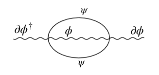
Figure 1: Two-loop contribution in the $\beta$ function of supersymmetric CP(1) model.

the $\phi$ fields without derivatives in the numerator in (152) and its complex conjugated are convoluted into the boson propagator.

Next, we split the calculation in two parts. First we evaluate the fermion loop depicted in Fig. 2. In $\mathds{C}P^{1}$ this is the same famous loop which appears in two-dimensional Schwinger model (Fig. 2).

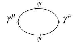
Figure 2: Fermion loop subdiagram.

Using

$$-i\,\frac{1}{2\pi}\,\frac{x_{\mu}\gamma^{\mu}}{x^{2}}\,\,\stackrel{{\scriptstyle\rm Fourier}}{{\longleftrightarrow}}\,\,\frac{ip_{\mu}\gamma^{\mu}}{p^{2}}$$ (153)

for the fermion propagator we obtain for the graph in Fig. 2

$$\frac{1}{2\pi^{2}}\,\frac{1}{x^{2}}\left(g^{\mu\nu}-\frac{2x^{\mu}x^{\nu}}{x^{2}}\right)\,\,\stackrel{{\scriptstyle\rm Fourier}}{{\longleftrightarrow}}\,\,\frac{i}{\pi}\left(\frac{p^{\mu}p^{\nu}}{p^{2}}-g^{\mu\nu}\right).$$ (154)

This is the famous Schwinger infrared effect.

Returning to the diagram in Fig. 1 we convince ourselves that the only actions still to be performed are to input the boson propagator $i/p^{2}$ and insert $(2/g^{2})^{2}$ for two vertices, $(g^{2}/2)^{3}$ for three propagators, $-2^{2}$ reflecting the factor of 2 in (152) and $-2$ in its complex conjugated, and the overall factor $-i$. The final result for the diagram in Fig. 1 is

$$\big{(}\partial_{\mu}\phi^{\dagger}\,\partial^{\mu}\phi\big{)}\,\frac{g^{2}}{2\pi^{2}}\,\log\frac{M_{0}}{\mu}$$ (155)

Since there is no second loop in ${\mathcal{N}}=(2,2)$ $\mathds{C}P^{1}$ model, this contribution must be canceled by the sum of all purely bosonic two-loop graphs. Hence, the two-loop renormalization in non-supersymmetric (purely bosonic) $\mathds{C}P^{1}$ model is

$$\delta{\mathcal{L}}=...-\big{(}\partial_{\mu}\phi^{\dagger}\,\partial^{\mu}\phi\big{)}\,\frac{g^{2}}{2\pi^{2}}\,\log\frac{M_{0}}{\mu}+...$$ (156)

where the dots stand for irrelevant contributions, $M_{0}$ is the UV cutoff and $\mu$ is the normalization point. Comparing $\delta{\mathcal{L}}$ above with $G\big{(}\partial_{\mu}\phi^{\dagger}\,\partial^{\mu}\phi\big{)}$ in (150) we arrive at the two-loop renormalization of the coupling constant in $\mathds{C}P^{1}$,

$$\delta\left(\frac{1}{g^{2}}\right)_{non\,\,{\rm SUSY\,}\mathds{C}P^{1}}=-\frac{g^{2}}{4\pi^{2}}\,\log\frac{M_{0}}{\mu}\,.$$ (157)

This result is certainly well-known in the literature Grah . What was not known is the fact that only one-loop in the graph is truly UV while the other comes from the IR and, therefore, this contribution would not be counted in the Wilsonean OPE.

The same conclusion is achieved from the instanton analysis.

References

- (1) S. Graham, Three-loop -function for the bosonic non-linear sigma model, Physics Letters B 197 (1987) 543.
- (2) A. Foakes and N. Mohammedi, Three-loop calculation of the beta-function for the purely metric non-linear sigma-model, Physics Letters B 198 (1987) 359.
- (3) A. Foakes and N. Mohammedi, An explicit three-loop calculation for the purely metric two-dimensional non-linear sigma model, Nuclear Physics B 306 (1988) 343.
- (4) S.V. Ketov, Quantum Non-linear Sigma-Models, Springer Berlin Heidelberg (2000), 10.1007/978-3-662-04192-5.
- (5) M. Nakahara, Geometry, Topology and Physics, IOP Publishes, 2nd edition, Bristol and Philadelphia (2004).
- (6) A.S. Losev, A. Marshakov and A.M. Zeitlin, On first-order formalism in string theory, Physics Letters B 633 (2006) 375 [hep-th/0510065].
- (7) A.A. Tseytlin, Sigma model renormalization group flow, “central charge” action, and perelman’s entropy, Physical Review D 75 (2007) [hep-th/0612296].
- (8) V.A. Novikov, M.A. Shifman, A.I. Vainshtein and V.I. Zakharov, Exact gell-mann-low function of supersymmetric yang-mills theories from instanton calculus, Nucl. Phys. B 229 (1983) 381.
- (9) M.A. Shifman and A. Vainshtein, Solution of the Anomaly Puzzle in SUSY Gauge Theories and the Wilson Operator Expansion, Nucl. Phys. B 277 (1986) 456.
- (10) X. Cui and M. Shifman, N=(0,2) deformation of the CP(1) model: Two-dimensional analog of N=1 Yang-Mills theory in four dimensions, Physical Review D 85 (2012) [1111.6350].
- (11) N. Arkani-Hamed and H. Murayama, Holomorphy, rescaling anomalies and exact functions in supersymmetric gauge theories, Journal of High Energy Physics 2000 (2000) 030 [hep-th/9707133].
- (12) A.V. Turbiner, One-dimensional quasi-exactly solvable schrödinger equations, Physics Reports 642 (2016) 1 [1603.02992].
- (13) M.A. Shifman, New Findings in Quantum Mechanics (Partial Algebraization of the Spectral Problem), Int. J. Mod. Phys. A 4 (1989) 2897.
- (14) D. Kutasov, String theory and the non-abelian thirring model, Physics Letters B 227 (1989) 68.
- (15) B. Gerganov, A. LeClair and M. Moriconi, Beta function for anisotropic current interactions in 2d, Phys. Rev. Lett. 86 (2001) 4753 [hep-th/0011189].
- (16) A.W. Ludwig and K.J. Wiese, The 4-loop -function in the 2d non-abelian thirring model, and comparison with its conjectured “exact” form, Nuclear Physics B 661 (2003) 577 [cond-mat/0211531].
- (17) A.M. Zeitlin, BRST, generalized maurer–cartan equations and CFT, Nuclear Physics B 759 (2006) 370 [hep-th/0610208].
- (18) A.M. Zeitlin, Perturbed beta–gamma systems and complex geometry, Nuclear Physics B 794 (2008) 381 [0708.0682].
- (19) A.M. Zeitlin, - systems and the deformations of the BRST operator, Journal of Physics A: Mathematical and Theoretical 42 (2009) 355401 [0904.2234].
- (20) N. Nekrasov, Lectures on curved beta-gamma systems, pure spinors, and anomalies, hep-th/0511008.
- (21) J.L. Cardy, Conformal invariance and statistical mechanics, in Les Houches Summer School in Theoretical Physics: Fields, Strings, Critical Phenomena, 1, 1989.
- (22) P.H. Ginsparg, Applied conformal field theory, in Les Houches Summer School in Theoretical Physics: Fields, Strings, Critical Phenomena, 9, 1988 [hep-th/9108028].
- (23) A.B. Zamolodchikov and A.B. Zamolodchikov, Conformal Field Theory and Critical Phenomena in Two-Dimensional Systems, New York, Harwood Academic (1989).
- (24) J. Zinn-Justin, Quantum Field Theory and Critical Phenomena, Oxford University Press (06, 2002), 10.1093/acprof:oso/9780198509233.001.0001.
- (25) C. Callan, D. Friedan, E. Martinec and M. Perry, Strings in background fields, Nuclear Physics B 262 (1985) 593.
- (26) C. Callan, I. Klebanov and M. Perry, String theory effective actions, Nuclear Physics B 278 (1986) 78.
- (27) E. Fradkin and A. Tseytlin, Quantum string theory effective action, Nuclear Physics B 261 (1985) 1.
- (28) D. Friedan, Nonlinear models in dimensions, Phys. Rev. Lett. 45 (1980) 1057.
- (29) D.H. Friedan, Nonlinear models in dimensions, Annals of Physics 163 (1985) 318.
- (30) J.O. Lye, A detailed look at the Calabi-Eguchi-Hanson spaces, 2201.07295.
- (31) C.M. Hull, Lectures on nonlinear sigma models and strings, in NATO Advanced Research Workshop on Superfield Theories, 7, 1986.
- (32) L. Baulieu, A.S. Losev and N.A. Nekrasov, Target space symmetries in topological theories i, Journal of High Energy Physics 2002 (2002) 021 [hep-th/0106042].
- (33) I. Affleck, D. Bykov and K. Wamer, Flag manifold sigma models, Physics Reports 953 (2022) 1 [2101.11638].
- (34) D.V. Bykov, Sigma models as Gross–Neveu models, Theoretical and Mathematical Physics 208 (2021) 993 [2106.15598].
- (35) D. Bykov, -function of the level-zero Gross-Neveu model, 2209.10502.
- (36) K. Sfetsos and K. Siampos, Gauged WZW-type theories and the all-loop anisotropic non-abelian thirring model, Nuclear Physics B 885 (2014) 583 [1404.7803].
- (37) K. Sfetsos, Integrable interpolations: From exact CFTs to non-abelian t-duals, Nuclear Physics B 880 (2014) 225 [1312.4560].
- (38) E. Sagkrioti, K. Sfetsos and K. Siampos, RG flows for -deformed CFTs, Nuclear Physics B 930 (2018) 499 [1801.10174].
- (39) O. Gamayun, A. Losev and A. Marshakov, First order string theory and the kodaira-spencer equations. I, Journal of High Energy Physics 2009 (2009) 028 [0906.4746].
- (40) O. Gamayun and A. Marshakov, First order string theory and the kodaira-spencer equations. II, Journal of High Energy Physics 2009 (2009) 065 [0907.1503].
- (41) G. Itsios, K. Sfetsos and K. Siampos, The all-loop non-Abelian Thirring model and its RG flow, Phys. Lett. B 733 (2014) 265 [1404.3748].
- (42) G. Georgiou, K. Sfetsos and K. Siampos, All-loop correlators of integrable -deformed -models, Nucl. Phys. B 909 (2016) 360 [1604.08212].
- (43) K. Stepanyantz, Derivation of the exact NSVZ -function in SQED, regularized by higher derivatives, by direct summation of feynman diagrams, Nuclear Physics B 852 (2011) 71 [1102.3772].
- (44) K.V. Stepanyantz, The NSVZ -function for theories regularized by higher covariant derivatives: the all-loop sum of matter and ghost singularities, Journal of High Energy Physics 2020 (2020) [1912.12589].
- (45) K.V. Stepanyantz, The all-loop perturbative derivation of the NSVZ -function and the NSVZ scheme in the non-abelian case by summing singular contributions, The European Physical Journal C 80 (2020) [2007.11935].
- (46) O. Gamayun, A. Losev and M. Shifman, work in progress, .
- (47) L. Alvarez-Gaumé and D.Z. Freedman, Kahler geometry and the renormalization of supersymmetric sigma models, Physical Review D 22 (1980) 846.
- (48) L. Alvarez-Gaume and D.Z. Freedman, Geometrical structure and ultraviolet finiteness in the supersymmetric sigma model, Commun. Math. Phys. 80 (1981) 443.
- (49) L. Alvarez-Gaume, D.Z. Freedman and S. Mukhi, The background field method and the ultraviolet structure of the supersymmetric nonlinear sigma model, Annals Phys. 134 (1981) 85.
- (50) V.A. Novikov, M.A. Shifman, A.I. Vainshtein and V.I. Zakharov, Two-Dimensional Sigma Models: Modeling Nonperturbative Effects of Quantum Chromodynamics, Phys. Rept. 116 (1984) 103.
- (51) M. Shifman, Perturbative proximity between supersymmetric and nonsupersymmetric theories, Phys. Rev. D 102 (2020) 125011.
- (52) E. Witten, String theory and black holes, Physical Review D 44 (1991) 314.
- (53) M. Shifman, Quantum Field Theory, Cambridge University Press, 2nd Edition (2022).