Comparison of indicators to evaluate the performance of climate models

Abstract

The evaluation of climate models is a crucial step in climate studies. It consists of quantifying the resemblance of model outputs to reference data to identify models with superior capacity to replicate specific climate variables. Clearly, the choice of the evaluation indicator significantly impacts the results, underscoring the importance of selecting an indicator that properly captures the characteristics of a "good model". This study examines the behavior of six indicators, considering spatial correlation, distribution mean, variance, and shape. A new multi-component measure was selected based on these criteria to assess the performance of 48 CMIP6 models in reproducing the annual seasonal cycle of precipitation, temperature, and teleconnection patterns in Central America. The top six models were determined using multi-criteria methods. It was found that even the best model reproduces one derived climatic variable poorly in this region. The proposed measure and selection method can contribute to enhancing the accuracy of climatological research based on climate models.

Keywords Climate models evaluation  $\cdot$ GCMs  $\cdot$ CMIP6  $\cdot$ Central America

1 Introduction

Climate models are complex mathematical representations of the components of the climate system [1]. Classified and ordered by their level of complexity, the General Circulation Models (GCMs) are located at the far end of the line. They are characterized by their global dominion and a large range of oceanic and atmospheric processes [2]. Considering that these models are developed by researchers in different laboratories across the globe under different methodologies and assumptions (including different physics and initializations), is not a surprise to find divergences in their projections[3]. The evaluation of these climate models consists on the analysis of the differences between these projections and a set of observed or reanalysis data [4], in order to identify the ones with the best capacity to reproduce a certain climatic characteristic in a specific spatial and temporal frame. It is evident that this performance is affected by the particular variable to be measured, the geographical area and the selected period, the data used as reference and finally the selected measure to quantify similarity [5]. Despite the plethora of available statistics to accomplish this evaluation task [6], there is not a standard method, because its selection will depend on the measurement purpose [7], which makes the exploration of new techniques still necessary [8]. A flaw in this exploration is the proposal of new measures without the assurance that they are capturing properly the characteristic of a “good model”. Of course, the definition of a “good model” is totally subjective, and can vary according to the goals settled, but at least, it must be specified for each evaluation method. In this study, the criteria proposed by Taylor [*]Taylor-2001 is used: a good model generates data that presents a high linear correlation with the reference set, besides similar variation and mean. Additional to these criteria, the similarity between the distributions shapes of the model output and the observed or reanalysis data is also contemplated. The importance of this last feature was pointed by Demirel et al. [10].

The model outputs used in this assessments are of a spatio-temporal nature. This means that every single data point is associated to a spatio-temporal location [11]. According to Wikle et al.[*]Wikle-2019 this kind of data can be seen as a sequence of static states or “pictures” (spatial perspective) or as a collection of time series (temporal perspective). This perspective is intrinsically related to the evaluation measures, which can be classified accordingly.

This research employs both spatial and temporal perspective methods, with the temporal approach relying on Functional Data Analysis (FDA) [13] - a statistical methodology that treats each indivisible unit of analysis as a function [14].

Our primary purpose is to evaluate the effectiveness of these measures in identifying a good model based on the Taylor criteria. This work also aims to determine which methods are suitable for generating ranking exercises using real climate model data from the Coupled Model Intercomparison Project (CMIP), currently in its sixth phase [15]. The structure of this article is as follows: Firstly, a description is provided for each of the techniques being considered. Next, the behavior of each technique is illustrated. Finally, based on these behaviors, a specific measure is chosen to evaluate 48 GCMs based on their ability to replicate the annual cycles for precipitation, temperature and influential teleconnections in Central America.

2 Data and Methods

2.1 Performance Measures

A completed and detailed list of measures to evaluate the performance of climatic models is beyond the scope of this work. However, after a thorough examination of various techniques, we have selected the following based on their potential ability to identify correlation and distribution similarities with reference data.

2.1.1 Skill Score

This is one of the most used methods to evaluate model performance. Proposed by Murphy [*]Murphy-1988, it is defined as the relative precision between two forecasts, fixing one of them as reference. Using the Mean Square Error (MSE) as the precision measure and recurring to the sample mean of the observed values as reference, the Skill Score of the model output $\mathbf{y}$ with respect to the observed values $\mathbf{x}$ is

$$SS(\mathbf{x},\mathbf{y})=\rho_{xy}^{2}-\Big{[}\rho_{xy}-\frac{s_{y}}{s_{x}}\Big{]}^{2}-\Big{[}\frac{\bar{y}-\bar{x}}{s_{x}}\Big{]}^{2}.$$

where $\rho_{xy}$ represents the linear correlation between the $\mathbf{x}$ and $\mathbf{y}$ vectors, $s_{x}$ and $s_{y}$ their standard deviations and $\bar{x}$ and $\bar{y}$ their respective means. The resulting values can vary from $-\infty$ to 1, being 1 the perfect score. Hidalgo and Alfaro [*]Hidalgo-2012 already applied this method to evaluate climate change projections in the Eastern Tropical Pacific Seascape and to rank CMIP5 models for reproducing characteristics of the seasonal cycles and El Niño-Southern Oscillation (ENSO) signal in Central America’s climate [18].

2.1.2 Spatial Efficiency

Demirel et al.[10] proposed the Spatial Efficiency (SPAEF) measure as an improvement of the Kling Gupta Efficiency (KGE) [19, 20], which is an attempt to correct some deficiencies of the Skill Score. It is conceived under a multi-objective approach in the calibration of hydrological models. It considers the Euclidean distance of three equally weighted components, as follows:

$$SPAEF(\mathbf{x},\mathbf{y})=1-\sqrt{(\alpha-1)^{2}+(\beta-1)^{2}+(\gamma-1)^{2}}$$

where $\alpha=\rho_{xy}$, $\beta=\frac{s_{y}/s_{x}}{\bar{y}/\bar{x}}$ and $\gamma=\sum_{b=1}^{B}\min(h_{xb},h_{yb})/\sum_{b=1}^{B}h_{xb}$. The last term represents the intersection of histograms $h_{x}$ and $h_{y}$ comparing their common $B$ bins, according to Swain & Ballard [21]. The range of values for this measure extends from $-\infty$ to 1, with a higher value closer to 1 denoting a stronger agreement with the reference data.

This indicator has been used by Ahmed et al. [22] in the ranking of GCMs in Pakistan.

2.1.3 Wasserstein Distance

The concept of Wasserstein distance (WD) arises from the optimal mass transportation problem and serves as a metric family specifically tailored for analyzing probability distributions [23]. It quantifies the cost of moving mass from one location to another. The WD of order $p$ between two probability distributions $P$ and $Q$ in $\mathbbm{R}^{d}$ is given by [24]:

$$WD(P,Q)=\inf\limits_{\begin{subarray}{c}X\sim P\ Y\sim Q\end{subarray}}(\mathbbm{E}|X-Y|)^{\frac{1}{p}}\quad p>0,$$

where $X$ and $Y$ are random variables following distributions $P$ and $Q$, respectively. If $P$ and $Q$ are the empirical distributions of $\mathbf{x}$ and $\mathbf{y}$, then the WD of order $p$ can be expressed as:

$$WD_{p}(\mathbf{x},\mathbf{y})=\Bigg{(}\sum_{i=1}^{n}|x_{i}-y_{i}|^{p}\Bigg{)}^{\frac{1}{p}}$$

$p=2$ is used in this study. As a distance metric, it takes values within the interval $[0,+\infty)$.

Vissio et al. [*]Vissio-2020 applied this distance in the evaluation of global-scale climate models.

2.1.4 Wasserstein Spatial Efficiency

As mentioned earlier, the effectiveness of a performance indicator in the context of this study, is subject to its capacity to identify spatial correspondence and differences between distributions: their position, dispersion and shape. The previous measures fail to detect at least one of these attributes. For example, SPAEF cannot quantify differences in the mean when the histogram intersection is applied to standardized vectors. On the other hand, WD is inadequate for measuring correlation since it does not consider the position of the values.. To address these limitations and provide a more comprehensive evaluation, we propose a novel measure that combines features from both indicators. This is accomplished by replacing the histogram intersection $\gamma$ in the SPAEF formulation by WD=$\phi$, because this distance is defined for not overlapping distributions [26], which allows to account for the bias. The Wasserstein Spatial Efficiency (WSPAEF) is the defined as:

$$WSPAEF(\mathbf{x},\mathbf{y})=\sqrt{(\alpha-1)^{2}+(\varsigma-1)^{2}+\phi^{2}}$$

where $\varsigma=s_{y}/s_{x}$, due the fact that Wasserstein distance is applied over the scaled vectors with variance equal to 1. The preference over the original $\beta$ term arises from its instability when the means approach zero. This instability can occur in the evaluation of dry or cold regions where precipitation or temperature values are low [27]. Initially, the utilization of Wasserstein distance (WD) emerged as a means to circumvent the cross-correlation issue associated with the bias component [28]. However, the incorporation of WD resolves this concern, rendering it irrelevant. The values assigned by this indicator range from 0 to $+\infty$ and can be interpreted as a distance from the reference set.

2.1.5 Kolmogorov Ranking Statistic

Harris et al. [*]Harris-2020 evaluate the similarity of two spatiotemporal fields using the concept of depth, specifically an adaptation of Tukey depth [*]Tukey-1975 to functional data. They proposed the Kolmogorov Depth Statistic (KD), which is effective in the detection of parameter’s changes and useful and pertinent for hypothesis testing purposes, but it does not go far enough if the final objective is to rank the distributions, when not only is necessary to test if there is a difference but also to determine the magnitude of this difference. For this reason, as an additional contribution of this article, the KD has been modified to quantify the misalignment between two function groups and to explore the behavior of temporal perspective techniques, resulting in the Kolmogorov Depth Ranking (KDPR) statistic.

As the KD authors explain, If $P$ is a distribution of a random variable $X\in C[0,1]^{p}$, and $P_{s}$ is the marginal distribution $P$ at location $s\in[0,1]^{p}$, the integrated Tukey depth of $X=x$ wrt $P$ is

$$D(x,P)=\int_{[0,1]^{p}}D(x(s),P_{s})ds$$

where $D(x(s),P_{s})$ is the univariate Tukey depth of $x(s)$ wrt to $P_{s}$, defined as $1-|1-2P(x(s))|$.

Consider two samples, $X\sim P$ and $Y\sim Q$, with estimators $P_{n}$ and $Q_{m}$ respectively. The outlyingness of any curve $x_{k}$ wrt to $P$ can be cuantified as:

$$\hat{F}_{X}(x_{k})=\frac{1}{n}\sum_{i=1}^{n}(D(x_{i},P_{n})-D(x_{k},P_{n}))$$

In the original form, this measure is a standardized rank of curves that follows a discrete uniform distribution [29]. However, this characteristic reduces its usefulness for ranking purposes.

In the same way as it was defined for $\hat{F}_{X}$, the outlyingness of any curve $y_{k}$ wrt to $P$ is:

$$\hat{G}_{Y}(x_{k})=\frac{1}{n}\sum_{j=1}^{n}(D(y_{j},P_{n})-D(x_{k},P_{n}))$$

Due, to the asymmetry property of depth, equivalent measures have to be calculated fixing $Q_{m}$.

$$\hat{F}_{X}(y_{k})=\frac{1}{n}\sum_{i=1}^{n}(D(x_{i},Q_{m})-D(y_{k},Q_{m}))$$

$$\hat{G}_{Y}(y_{k})=\frac{1}{n}\sum_{j=1}^{n}(D(y_{j},Q_{m})-D(y_{k},Q_{m}))$$

The Kolmogorov distance is utilized to compute the KDPR statistic by summing the differences between the “intra” outlyingness measures ($\hat{F}_{X}(x_{k})$, $\hat{G}_{Y}(y_{k})$) and their “inter” counterparts ($\hat{F}_{X}(y_{k})$, $\hat{G}_{Y}(x_{k})$):

$$KDPR(X,Y)=\max\left[\sum\hat{F}_{X}(x_{k})-\hat{G}_{Y}(x_{k}),\sum\hat{F}_{X}(y_{k})-\hat{G}_{Y}(y_{k})\right]$$

The same approach can be applied by substituting depth with alternative distances, (Kolmogorov Distance Ranking or KDSR). For instance, $\hat{F}_{X}(x_{k})$ can be redefined as:

$$\hat{F}_{X}(x_{k})=\frac{1}{n}\sum_{i=1}^{n}||x_{i}-x_{k}||$$

The range of both versions extends from 0 to $+\infty$, where 0 represents a perfect match between observed-reanalysis and simulated data.

2.2 Measures Behavior

To establish our definition of a “good model”, a measure should operate in the following manner when comparing model and reference sets: it should exhibit an increase in value as the correlation between the sets diminishes and the discrepancies in means and variations widen. Additionally, greater values are expected if the empirical distributions of the sets are not similar in terms of their forms. While the SS behavior can be analytically described in a trivial manner, this is not the case for the rest of the techniques, therefore, it is necessary to generate synthetic data to show their behavior. The realizations $\mathbf{x}$ and $\mathbf{y}$ of two spatiotemporal fields $X$ and $Y$ were compared under the resulting combinations of the following characteristics: (a) Linear correlation ($\rho=\rho_{xy}$): -0.9, -0.3, 0.3, 0.9. (b) Standard deviation ratio ($\lambda=\frac{s_{y}}{s_{x}}$): 0.1, 0.7, 1.0, 1.3, 1.9. (c) Bias ($\delta=|\bar{x}-\bar{y}|$): 0.0, 1.0, 5.0. To achieve this, preliminary samples $\mathbf{x^{\prime}}$ and $\mathbf{y^{\prime}}$ were first obtained, which also come from the aforementioned fields $X$ and $Y$, respectively. These consist of sets of 100 static states (temporal segments) of size $5\times 5$, generated using an isotropic and stationary covariance model from the Matérn family, according to the equation:

$$C(r)=\frac{2^{1-\nu}}{\Gamma{\nu}}(\sqrt{2\nu r})^{\nu}K_{\nu}(\sqrt{2\nu r})$$

where $r$ is the distance between two points, $\nu$ is the smoothing parameter ($\nu=1.5$ in this design), and $K_{\nu}$ is the modified Bessel function of the second kind [31]. In addition to the established scenarios, two conditions were created: “Undisturbed” where the shape of the empirical distribution of the preliminary samples $\mathbf{x^{\prime}}$ or $\mathbf{y^{\prime}}$ is not altered, and “Disturbed” where a log-normal transformation ($\mu=1$ and $\sigma=0.5$) is applied to $\mathbf{x^{\prime}}$. For each combination, the data composing $\mathbf{x^{\prime}}$ and $\mathbf{y^{\prime}}$ were organized into centered vectors $\mathbf{u}$ and $\mathbf{v}$. Using $\mathbf{u}$ as a reference and considering that correlation is the magnitude of the cosine of the angle $\theta$ between two centered vectors [32], a new vector $\mathbf{w}$ was generated, defined as:

$$\mathbf{w}=\rho_{uw}\frac{\mathbf{v}_{\parallel\mathbf{u}}}{\|\mathbf{v}_{\parallel\mathbf{u}}\|}+\sqrt{1-\rho_{uw}^{2}}\frac{\mathbf{v}_{\perp\mathbf{u}}}{\|\mathbf{v}_{\perp\mathbf{u}}\|}$$

where $\rho_{uw}$ is the desired correlation between the vectors $\mathbf{u}$ and $\mathbf{w}$, $\mathbf{v}_{\parallel\mathbf{u}}$ is the projection of $\mathbf{v}$ onto $\mathbf{u}$, and $\mathbf{v}_{\perp\mathbf{u}}=\mathbf{v}-\mathbf{v}_{\parallel\mathbf{u}}$ is the projection of $\mathbf{v}$ onto the orthogonal complement of $\mathbf{u}$. Since correlation is not affected by linear transformations, the reference vector $\mathbf{x}=\frac{\mathbf{u}}{s_{u}+c}$ and the vector $\mathbf{y}=\frac{\mathbf{w}}{s_{w}\lambda+c+\delta}$ were defined such that $\lambda=\frac{s_{y}}{s_{x}}$, $\delta=|\bar{x}-\bar{y}|$ (as required), and $\rho_{uw}=\rho_{xy}$. The constant $c$ is arbitrary, as the interest lies in the relationships between certain characteristics of the samples rather than their values. In this case, $c=10$ (because of the issues related to some indicators when the mean is close to 0). Finally, the selected techniques were applied to the pair of vectors $\mathbf{x}$ and $\mathbf{y}$ in each case, considering the entire temporal extension.

Starting by the SS indicator (Figure 1), as a desirable feature, it shows high sensitivity to bias and correlation, however, only in high positive correlation scenarios the lowest point in each facet correspond to the best model in terms of variability, in any other case, the measure will be oriented to models with lower standard deviations than the reference. The SPAEF (Figure 2) corrects this last characteristic, but just for models with non discrepancies in the mean. When these discrepancies increase, the SPAEF privileges models with higher variability (relative to the reference). Other problems are the lack of sensitivity to the mean and shape dissemblance. The first issue was pointed out previously, but the second one was expected to be captured with the $\gamma$ component, which is its main feature over the SS or other measures as the Kling Gupta Efficiency. The WD (Figure 3) detects effectively the bias, variability (with certain level of asymmetry) and shape but, as mentioned, it does not consider the linear correlation. Adding dimensions solve this last issue, but the resulting behavior is almost identical to the skill score. The WSPAEF (Figure 4) seems to meet all the requirements. The weight of mean difference and the correlation value is clearly greater that dissimilarities in variation and shape, which can be seem as a desirable feature depending of the application. Finally, the modified Kolmogorov depth (Figure 5) works relative well when $\delta=0$ but for greater values the behavior change radically until achieving even a concave form. The distance version (Figure 5), leaving aside certain asymmetry, behaves properly when the bias is low. One can said that, in that specific condition, it is the best option to consider if the primary interest is to detect differences in variability.

In ranking methodologies, the lack of a “true model” for ranking, makes impossible the calculation of an accuracy indicator [33], however, the patterns analyzed indicates that the WSPAEF is the best option to proceed with the model sorting exercise if the Taylor criteria is used as a guideline.

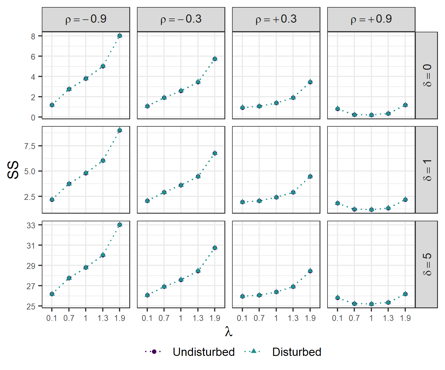
Figure 1: Skill score behavior

Notes: $\rho$: linear correlation, $\lambda$: variation ratio, $\delta$: bias. The “Undisturbed” series refers to normal data while the “Disturbed” series refers to a log-normal transformation of this data. Lower values indicates a better model.

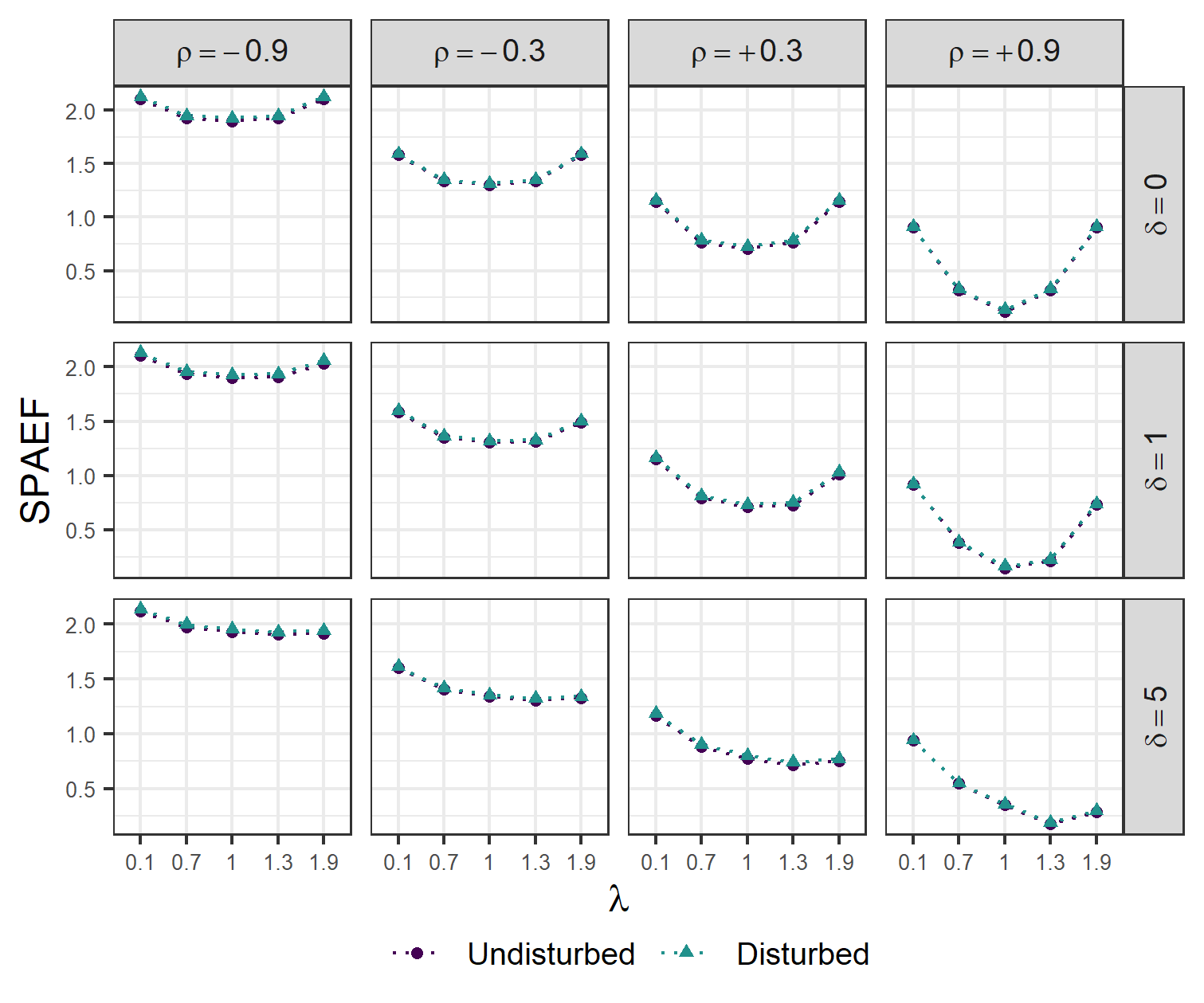
Figure 2: SPAEF behavior

Notes: $\rho$: linear correlation, $\lambda$: variation ratio, $\delta$: bias. The “Undisturbed” series refers to normal data while the “Disturbed” series refers to a log-normal transformation of this data. Lower values indicates a better model.

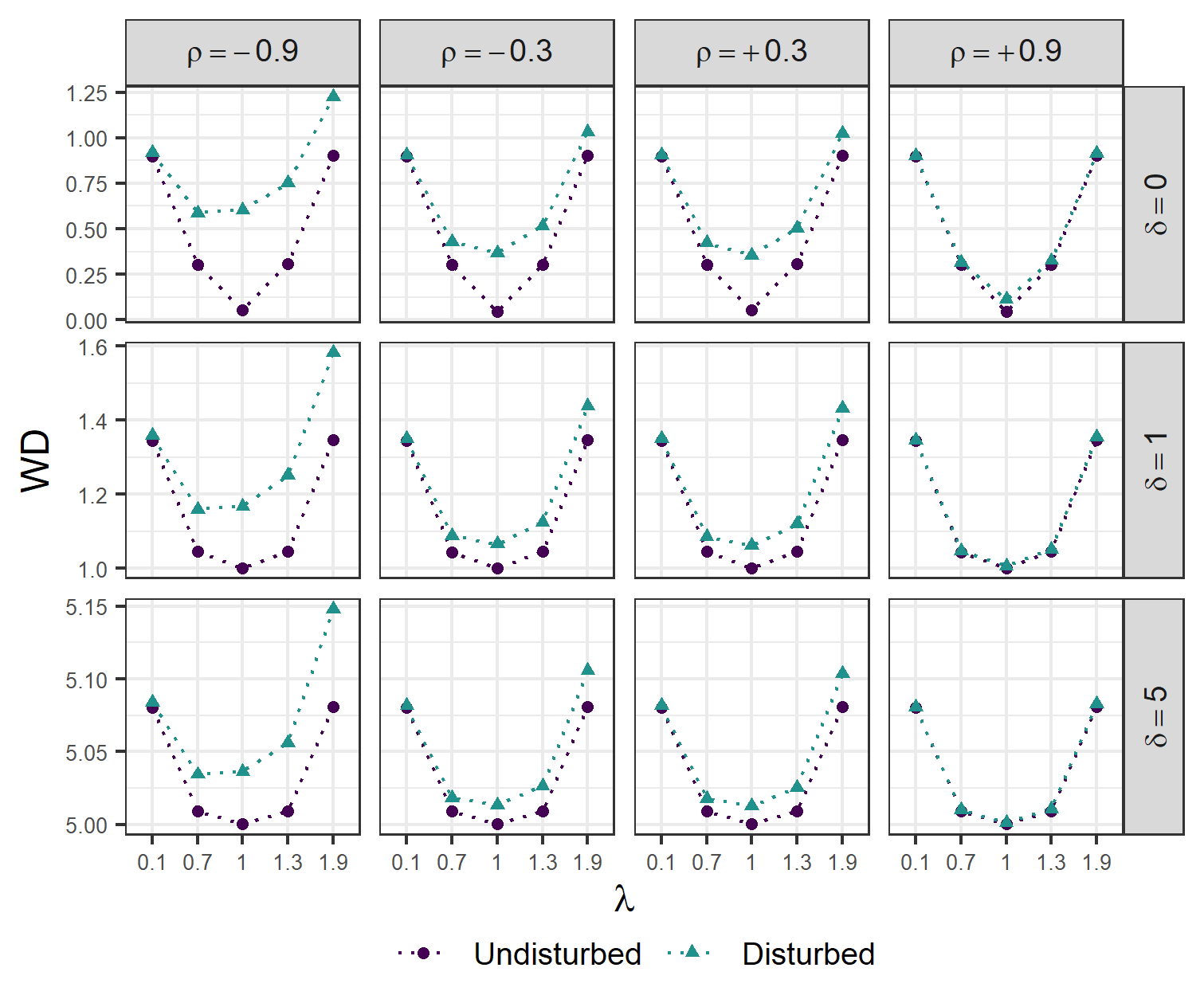
Figure 3: Wasserstsein distance behavior

Notes: $\rho$: linear correlation, $\lambda$: variation ratio, $\delta$: bias. The “Undisturbed” series refers to normal data while the “Disturbed” series refers to a log-normal transformation of this data. Lower values indicates a better model.

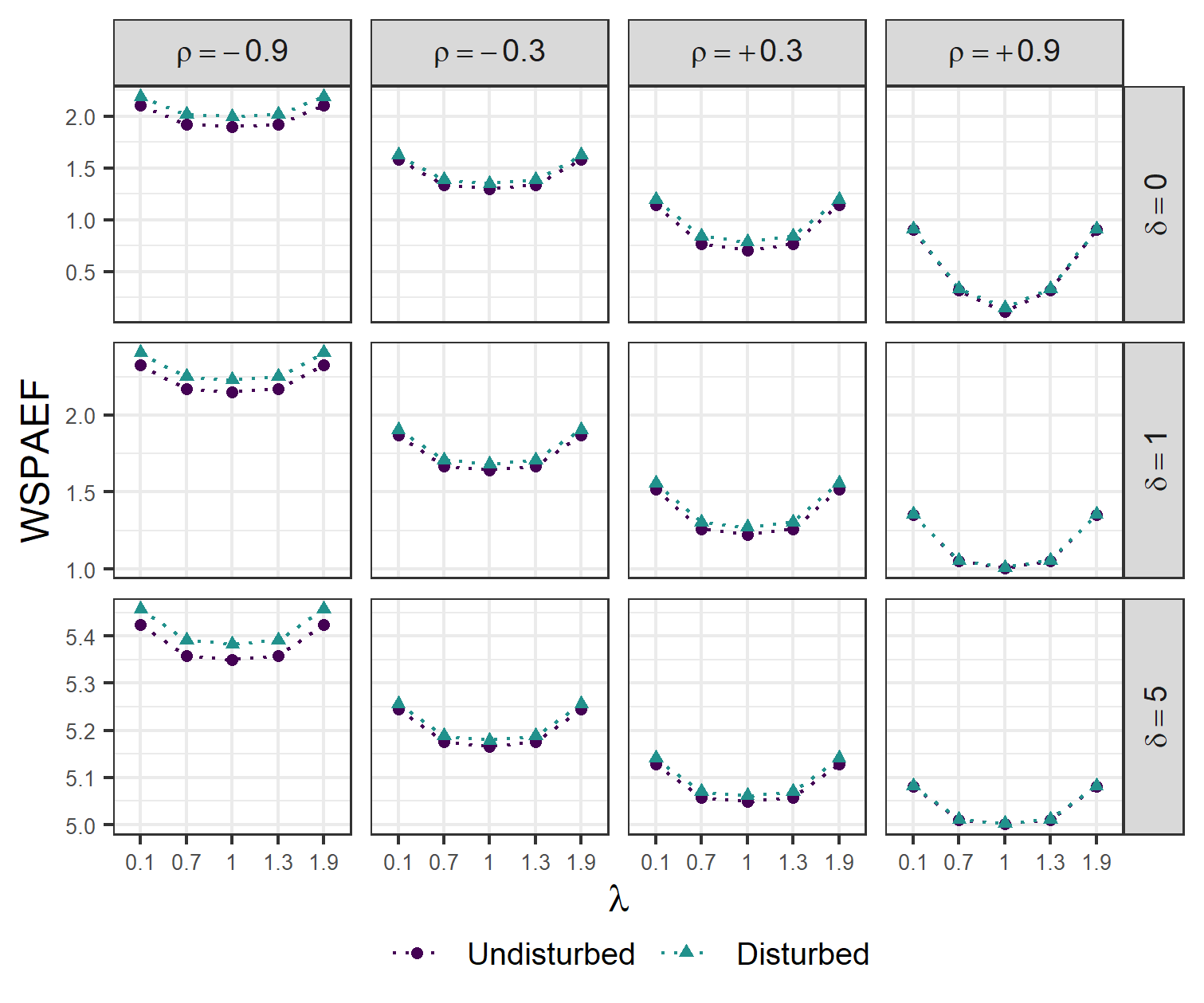
Figure 4: Wasserstein SPAEF

Notes: $\rho$: linear correlation, $\lambda$: variation ratio, $\delta$: bias. The “Undisturbed” series refers to normal data while the “Disturbed” series refers to a log-normal transformation of this data. Lower values indicates a better model.

Figure 5: Kolmogorov depth

Notes: $\rho$: linear correlation, $\lambda$: variation ratio, $\delta$: bias. The “Undisturbed” series refers to normal data while the “Disturbed” series refers to a log-normal transformation of this data. Lower values indicates a better model.

Figure 6: Kolmogorov distance

Notes: $\rho$: linear correlation, $\lambda$: variation ratio, $\delta$: bias. The “Undisturbed” series refers to normal data while the “Disturbed” series refers to a log-normal transformation of this data. Lower values indicates a better model.

2.3 Application

The chosen indicator will be utilized for evaluating the monthly outputs of precipitation and temperature variables from 48 CMIP6 models. For precipitation, the reference data is part of the Global Precipitation Climatology Project version 2.3 dataset [34]. These data include measurements from sensors and satellites from 1979 to the present, covering a global grid (88.75°N-88.75°S, 1.25°E-358.75°E) with a resolution of 2.5°. The temperature data is obtained from reanalysis data provided by the National Centers for Environmental Prediction (NCEP) and the National Center for Atmospheric Research (NCAR) [35]. The temporal coverage is from 1948 to the present, and the spatial coverage is 90°N-90°S, 0°E-357.5°E, with a resolution of 2.5°. A sea surface temperature dataset from the National Oceanic and Atmospheric Administration (NOAA) [36] is also used to gauge El Niño South Oscilation (ENSO) and Tropical North Atlantic (TNA) teleconnection patterns. It contains temperature measurements from ships and buoys from 1854 to the present, covering the area from 88°N-88°S, 0°E-358°E, with a resolution of 2.0°. The model data was obtained from the World Climate Research Program (WCRP). The complete list of models can be seen in Table 1. The model run indicates the realization (r), initialization method (i), physics (p), and forcing (f) used. All the models were transformed to a 2.5°resolution to match the observed data using bilinear interpolation.

The area under study (4°N-20°N, 95°W-75°W), as well as the teleconnection regions can be seen in Figure 7. The temporal frame of the study is limited to the period from 1979 to 1999.

The comparison will focus on the annual seasonal cycles rather than the entire spatio-temporal field, resulting in the derivation of new variables. To illustrate, by computing the mean precipitation values for each grid point in January and repeating this process for the other months, we can obtain the annual cycle of mean precipitation. In this study, in addition to the provided example, the annual cycle of standard deviations for precipitation and their analogues for surface temperature were also used. The resulting derived variables are: precipitation mean (PRM), precipitation standard deviation (PRS), temperature mean (TPM) and temperature standard deviation (TPS). The teleconnection patterns were generated using the procedure proposed by Hidalgo and Alfaro (2015). For each season (December-January-February [DJF], March-April-May [MAM], June-July-August [JJA], September-October-November [SON]), the temporal correlation between the sea surface temperature time series and the precipitation series within the study region is calculated. These correlations are then combined to form teleconnection variables such as ENSO (El Niño-Southern Oscillation) and TNA (Tropical North Atlantic). The WSPAEF values for each month or season in the annual cycle can be combined using the euclidean norm.

Figure 7: Geographical area under study

Table 1: Preselected model and runs

No	Model	Run	Institution	Resolution
1	CMCC-CM2-HR4	r1i1p1f1	Fondazione Centro Euro-Mediterraneo sui Cambiamenti Climatici (FCEMCC)	111 km
2	CMCC-CM2-VHR4	r1i1p1f1	FCEMCC	25 km
3	CNRM-CM6-1	r1i1p1f2	CNRM-CERFACS	250 km
4	CNRM-CM6-1	r2i1p1f2	CNRM-CERFACS	250 km
5	CNRM-CM6-1	r3i1p1f2	Centre National de Recherches Meteorologiques (CNRM), Centre Europeen de Recherche et de Formation Avancee en Calcul Scientifique (CERFACS)	250 km
6	CNRM-CM6-1-HR	r1i1p1f2	CNRM-CERFACS	50 km
7	EC-Earth3P	r1i1p2f1	EC-Earth consortium	100 km
8	EC-Earth3P	r2i1p2f1	EC-Earth	100 km
9	EC-Earth3P	r3i1p2f1	EC-Earth	50 km
10	EC-Earth3P-HR	r1i1p2f1	EC-Earth	50 km
11	EC-Earth3P-HR	r2i1p2f1	EC-Earth	50 km
12	EC-Earth3P-HR	r3i1p2f1	EC-Earth	50 km
13	ECMWF-IFS-HR	r1i1p1f1	European Centre for Medium-Range Weather Forecasts (ECMWF)	25 km
14	ECMWF-IFS-HR	r2i1p1f1	ECMWF	25 km
15	ECMWF-IFS-HR	r3i1p1f1	ECMWF	25 km
16	ECMWF-IFS-HR	r4i1p1f1	ECMWF	25 km
17	ECMWF-IFS-HR	r5i1p1f1	ECMWF	25 km
18	ECMWF-IFS-HR	r6i1p1f1	ECMWF	25 km
19	ECMWF-IFS-LR	r1i1p1f1	ECMWF	50 km
20	ECMWF-IFS-LR	r2i1p1f1	ECMWF	50 km
21	ECMWF-IFS-LR	r3i1p1f1	ECMWF	50 km
22	ECMWF-IFS-LR	r4i1p1f1	ECMWF	50 km
23	ECMWF-IFS-LR	r5i1p1f1	ECMWF	50 km
24	ECMWF-IFS-LR	r6i1p1f1	ECMWF	50 km
25	ECMWF-IFS-LR	r7i1p1f1	ECMWF	50 km
26	ECMWF-IFS-LR	r8i1p1f1	ECMWF	50 km
27	ECMWF-IFS-MR	r1i1p1f1	ECMWF	50 km
28	ECMWF-IFS-MR	r2i1p1f1	ECMWF	50 km
29	ECMWF-IFS-MR	r3i1p1f1	ECMWF	50 km
30	GFDL-CM4C192	r1i1p1f1	Geophysical Fluid Dynamics Laboratory (NOAA-GFDL)	100 km
31	HadGEM3-GC31-HH	r1i1p1f1	Natural Environment Research Council (NERC)	50 km
32	HadGEM3-GC31-HM	r1i1p1f1	Met Office Hadley Centre (MOHC)	50 km
33	HadGEM3-GC31-HM	r1i2p1f1	NERC	50 km
34	HadGEM3-GC31-HM	r1i3p1f1	MOHC	50 km
35	HadGEM3-GC31-LL	r1i1p1f1	MOHC	250 km
36	HadGEM3-GC31-LL	r1i2p1f1	MOHC	250 km
37	HadGEM3-GC31-LL	r1i3p1f1	MOHC	250 km
38	HadGEM3-GC31-LL	r1i4p1f1	MOHC	250 km
39	HadGEM3-GC31-LL	r1i5p1f1	MOHC	250 km
40	HadGEM3-GC31-LL	r1i6p1f1	MOHC	250 km
41	HadGEM3-GC31-LL	r1i7p1f1	MOHC	250 km
42	HadGEM3-GC31-LL	r1i8p1f1	MOHC	250 km
43	HadGEM3-GC31-MM	r1i1p1f1	MOHC	100 km
44	HadGEM3-GC31-MM	r1i2p1f1	MOHC	100 km
45	HadGEM3-GC31-MM	r1i3p1f1	MOHC	100 km
46	INM-CM5-H	r1i1p1f1	Institute for Numerical Mathematics (INM-RAS)	100 km
47	MPI-ESM1-2-HR	r1i1p1f1	Max Planck Institute for Meteorology (MPIM)	100 km
48	MPI-ESM1-2-XR	r1i1p1f1	MPIM	50 km

2.4 Model Ranking

Given that the performance of each model is assessed based on multiple derived variables, the selection and ordering of these variables present a multicriteria decision problem. In the realm of Global Climate Model (GCM) evaluation, there is no consensus on a specific method. Therefore, three different methods were employed: the Euclidean norm (L2N) as a control, the Technique for Order Preference by Similarity to Ideal Solution (TOPSIS) proposed by [37], and the Preference Ranking Organization Method for Enrichment of Evaluations (PROMETHEE) introduced by [38]. These choices were made based on their popularity, properties, different approaches [39], and previous use in similar studies [6, 40, 41, 42]. Finally, the coincident models within the top eight positions according to each of these final rankings were selected.

The following describes each of these methods. Let $A=\{a_{1},a_{2},...,a_{n}\}$ be a set of $n$ models or alternatives, and $F=\{f_{1},f_{2},...,f_{m}\}$ be a set of $m$ variables or criteria that should be minimized. They are organized as follows:

$$\begin{pmatrix}f_{1}(a_{1})&f_{2}(a_{1})&\cdots&f_{m}(a_{1})\\ f_{1}(a_{2})&f_{2}(a_{2})&\cdots&f_{m}(a_{2})\\ \vdots&\vdots&\ddots&\vdots\\ f_{1}(a_{n})&f_{2}(a_{n})&\cdots&f_{m}(a_{n})\end{pmatrix}$$

2.4.1 Euclidean Norm (L2N)

The concept of Euclidean norm or L2-norm is used to calculate the distance from a model $a$ to the origin or point 0 in an $m$-dimensional space, as follows:

$$d_{a}=\sqrt{\sum_{j=1}^{m}(f_{j}(a))^{2}}$$

These distance values are used for ranking operation; the best models are those located at a shorter distance from the origin in the $\mathbbm{R}^{m}$ space.

2.4.2 TOPSIS

This method also relies on Euclidean distance, but instead of using 0 as a reference point, it uses the positive and negative ideal solutions for each variable, represented by $f_{j}(\cdot)^{+}$ and $f_{j}(\cdot)^{-}$, respectively, which correspond to the minimum and maximum values of each column. The distances of each model to these values are then calculated as:

$$d_{a}^{+}=\sqrt{\sum_{j=1}^{m}(f_{j}(a)-f_{j}(\cdot)^{+})^{2}}$$

$$d_{a}^{-}=\sqrt{\sum_{j=1}^{m}(f_{j}(a)-f_{j}(\cdot)^{-})^{2}}$$

Then, the normalized score $\xi_{a}=d_{a}^{-}/(d_{a}^{-}+d_{a}^{+})$ is used to rank the alternatives. A perfect value of 1 will be assigned to the best alternative and 0 to the worst one, so the models with higher scores are considered of superior performance and occupy a lower position in the ranking. The complete description of this process can be found in Lai et al. [37].

2.4.3 PROMETHEE

This method compares two alternatives $\{a,a^{*}\}\in A$ using a preference function $P_{j}(a,a^{*})$. This function depends on the difference between the evaluations of $a$ and $a^{*}$, expressed as $\Delta_{j}(a,a^{*})=f_{j}(a)-f_{j}(a^{*})$. Although there are various types of preference functions, this study opted for the “usual function” [38], described as:

$$P_{j}(a,a^{*})=\begin{cases}0&\quad\text{if }\Delta_{j}(a,a^{*})\geq 0\\ 1&\quad\text{if }\Delta_{j}(a,a^{*})<0\\ \end{cases}$$

When using this function, it indicates that $a$ is strictly preferred to $a^{*}$ for any negative $\Delta_{j}(a,a^{*})$. Model ranking is performed based on the score $\Phi(a)$, defined as:

$$\Phi(a)=\frac{\sum_{a^{*}\in A}\pi(a,a^{*})}{n-1}-\frac{\sum_{a^{*}\in A}\pi(a^{*},a)}{n-1}$$

where $\pi(a,a^{*})$ represents the weighted average of the preference functions:

$$\pi(a,a^{*})=\frac{\sum_{j=1}^{m}\omega_{j}P_{j}(a,a^{*})}{\sum_{j=1}^{m}\omega_{j}}$$

Similar to TOPSIS, higher score values are associated with better models. For a detailed version of the general procedure, refer to Brans et al. [*]Brans-1986.

3 Results

Table 2 presents the ranking for each of the six derived variables, along with the three final rankings obtained using the L2N, TOPSIS, and PROMETHEE methods. The table is not sorted based on the result of a particular method since none can be considered “true”. When evaluating the Spearman correlations of TOPSIS and PROMETHEE with respect to L2N, correlation values of 0.96 and 0.89 were obtained, respectively, while the correlation between TOPSIS and PROMETHEE was 0.86. These values indicate that the results are similar and consistent. If this were not the case, each ranking method could be questioned [39].

Table 2: Model position by variable and ranking method

No.	Model	Run	PRM	PRS	TPM	TPS	ENSO	TNA	L2N	TOPSIS	PROMETHEE
1	CMCC-CM2-HR4	r1i1p1f1	48	47	35	26	5	4	47	48	32
2	CMCC-CM2-VHR4	r1i1p1f1	47	46	36	4	47	48	48	47	48
3	CNRM-CM6-1	r1i1p1f2	25	7	41	27	9	7	25	28	12
4	CNRM-CM6-1	r2i1p1f2	24	15	38	9	17	27	30	30	16
5	CNRM-CM6-1	r3i1p1f2	26	17	40	45	28	22	34	35	38
6	CNRM-CM6-1-HR	r1i1p1f2	13	37	48	35	23	16	36	36	35
7	EC-Earth3P	r1i1p2f1	29	43	31	36	13	21	33	34	36
8	EC-Earth3P	r2i1p2f1	31	45	34	43	39	24	40	42	44
9	EC-Earth3P	r3i1p2f1	28	42	29	44	2	17	24	32	30
10	EC-Earth3P-HR	r1i1p2f1	2	40	28	2	27	37	14	18	20
11	EC-Earth3P-HR	r2i1p2f1	4	41	1	16	1	13	1	1	2
12	EC-Earth3P-HR	r3i1p2f1	3	39	27	11	14	9	9	15	10
13	ECMWF-IFS-HR	r1i1p1f1	1	23	18	17	4	14	2	4	3
14	ECMWF-IFS-HR	r2i1p1f1	19	21	24	1	20	6	8	9	7
15	ECMWF-IFS-HR	r3i1p1f1	17	33	23	10	3	1	4	8	6
16	ECMWF-IFS-HR	r4i1p1f1	18	36	20	14	16	44	16	20	26
17	ECMWF-IFS-HR	r5i1p1f1	11	16	19	3	25	8	7	5	5
18	ECMWF-IFS-HR	r6i1p1f1	12	35	22	23	44	39	27	22	37
19	ECMWF-IFS-LR	r1i1p1f1	36	27	45	31	30	20	39	39	39
20	ECMWF-IFS-LR	r2i1p1f1	38	29	39	38	31	18	41	40	40
21	ECMWF-IFS-LR	r3i1p1f1	34	19	37	40	24	46	37	38	41
22	ECMWF-IFS-LR	r4i1p1f1	44	26	47	19	40	43	46	44	46
23	ECMWF-IFS-LR	r5i1p1f1	35	30	42	37	42	36	44	41	47
24	ECMWF-IFS-LR	r6i1p1f1	45	25	46	41	10	47	43	46	43
25	ECMWF-IFS-LR	r7i1p1f1	42	31	44	32	38	30	45	43	45
26	ECMWF-IFS-LR	r8i1p1f1	37	34	43	29	21	2	38	37	33
27	ECMWF-IFS-MR	r1i1p1f1	21	5	21	42	26	23	21	21	22
28	ECMWF-IFS-MR	r2i1p1f1	33	22	26	6	48	34	35	29	34
29	ECMWF-IFS-MR	r3i1p1f1	32	18	25	8	8	11	12	19	9
30	GFDL-CM4C192	r1i1p1f1	20	28	33	28	7	19	15	27	18
31	HadGEM3-GC31-HH	r1i1p1f1	41	3	15	7	41	28	31	23	19
32	HadGEM3-GC31-HM	r1i1p1f1	40	6	3	5	19	5	18	14	4
33	HadGEM3-GC31-HM	r1i2p1f1	43	9	4	18	22	25	28	26	14
34	HadGEM3-GC31-HM	r1i3p1f1	39	1	6	34	11	41	23	25	17
35	HadGEM3-GC31-LL	r1i1p1f1	9	13	12	15	32	15	5	3	8
36	HadGEM3-GC31-LL	r1i2p1f1	6	32	13	13	37	38	11	11	23
37	HadGEM3-GC31-LL	r1i3p1f1	10	20	17	22	34	33	10	10	21
38	HadGEM3-GC31-LL	r1i4p1f1	16	11	8	25	6	3	3	2	1
39	HadGEM3-GC31-LL	r1i5p1f1	5	38	16	20	18	29	6	7	15
40	HadGEM3-GC31-LL	r1i6p1f1	14	14	9	24	45	35	20	13	24
41	HadGEM3-GC31-LL	r1i7p1f1	8	10	5	12	46	32	13	6	11
42	HadGEM3-GC31-LL	r1i8p1f1	15	44	7	21	36	26	19	16	27
43	HadGEM3-GC31-MM	r1i1p1f1	23	2	10	46	29	45	22	24	28
44	HadGEM3-GC31-MM	r1i2p1f1	27	4	14	30	43	40	26	17	29
45	HadGEM3-GC31-MM	r1i3p1f1	22	8	11	33	35	12	17	12	13
46	INM-CM5-H	r1i1p1f1	30	48	2	39	15	10	29	33	25
47	MPI-ESM1-2-HR	r1i1p1f1	7	12	32	48	33	31	32	31	31
48	MPI-ESM1-2-XR	r1i1p1f1	46	24	30	47	12	42	42	45	42

Six models were found to be in common among the top eight positions in all three multi-criteria methods. These are shown in Figure 8 with their respective positions. Based on the criteria used, it can be asserted that any of these models are capable of adequately reproducing the annual cycle of the analyzed variables.

Model 11 (EC-Earth3P-HR r2i1p2f1) is the best according to L2N and TOPSIS, and the second best according to PROMETHEE, thanks to its ability to reproduce TPM and ENSO. However, it should be noted that it ranks 41st for the PRS variable. This should be taken into consideration if this variable is of special interest. Other more balanced alternatives are Model 13 (ECMWF-IFS-HR r1i1p1f1) and Model 38 (HadGEM3-GC31-LL r1i4p1f1). Notice that all selected models occupy relatively high positions in at least one variable.

Figure 8: Selected models positions

Figures 9 and 10 show the model performance for the temporal grouping of the annual cycle. For mean precipitation, in general, all models show better performance during the drier months (Jan - Mar) and also less variability among them [43]. The same pattern is repeated for the standard deviation, although less prominently. For mean temperature, the WSPAEF values consistently increase until reaching a maximum in June and then decrease. On the other hand, the variability of the results seems to remain constant throughout the cycle. It can also be observed that Model 11 consistently ranks at the minimum or near-minimum positions in all months, justifying its position in the ranking for this variable. TPS does not exhibit any clear trend, but it is worth noting its overall good performance for the month of November and the opposite for February.

The teleconnection patterns (Figure 10), segregated by region, do not show clear trends and appear to be fairly stable. However, the selected individual models exhibit an interesting phenomenon. Model 11, which ranks first overall for ENSO, seems to perform poorly for the MAM season, whereas Model 35, which ranks last for this variable among the selected models, performs particularly well for this season.

Although other studies have evaluated CMIP6 GCMs in Central America [44, 45], differences in the choice of spatial and temporal domains, variables under analysis, reference datasets, and performance indicators, among others, prevent a direct comparison. Additionally, the preselection of models and their respective runs was not the same, further reducing the likelihood of coincidences. With this in mind, it is important to highlight that at least one model from the EC-Earth consortium (EC-Earth3P-HR) shows superior performance in this study and previous studies (EC-Earth3 and EC-Earth3-Veg).

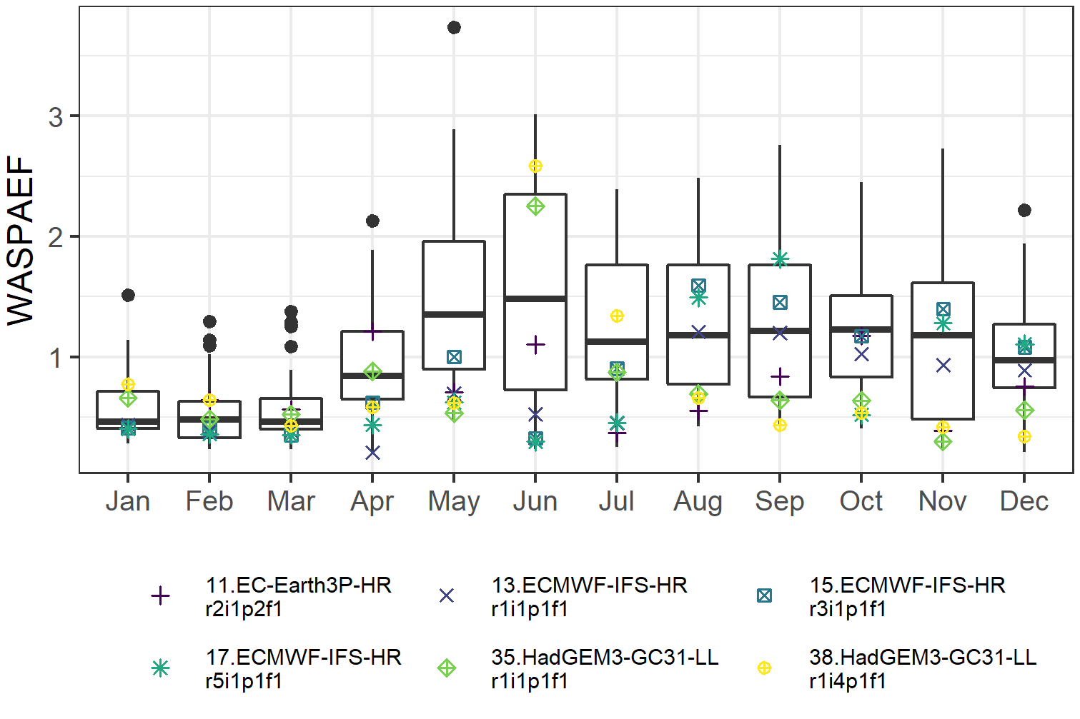
(a) PRM

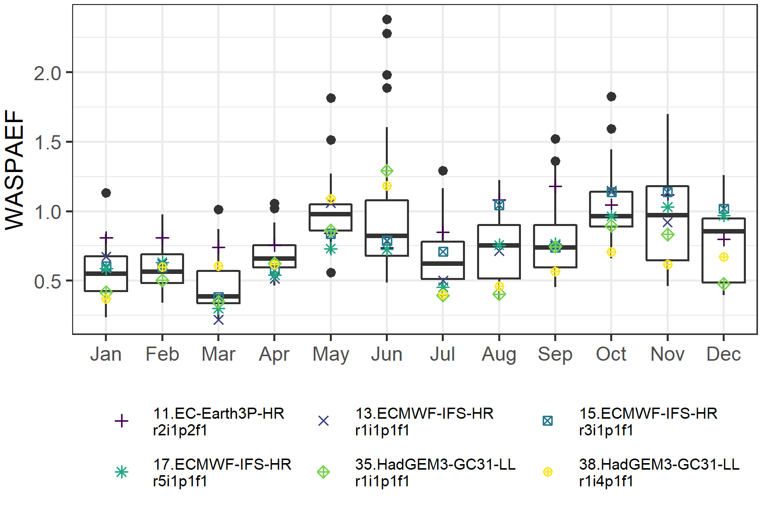
(b) PRS

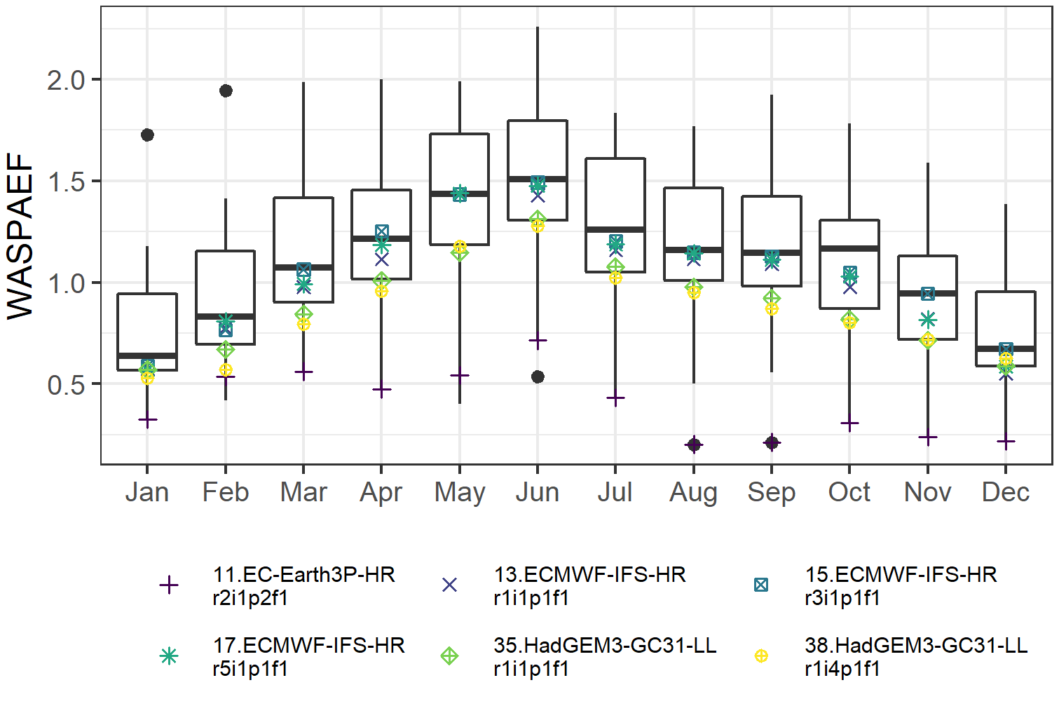
(c) TPM

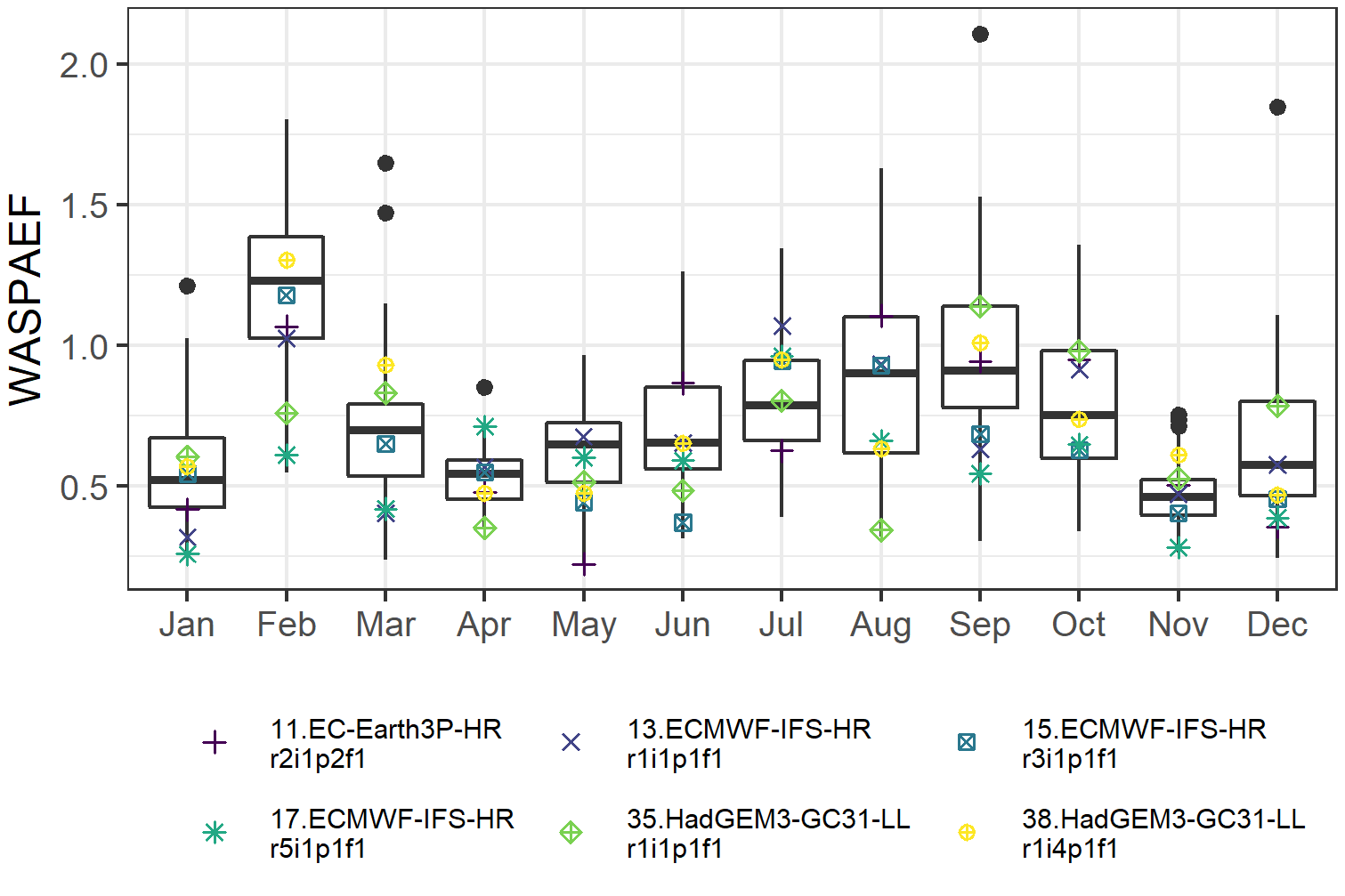
(d) TPS

Figure 9: Precipitation and temperature derived variables WSAPEF by month

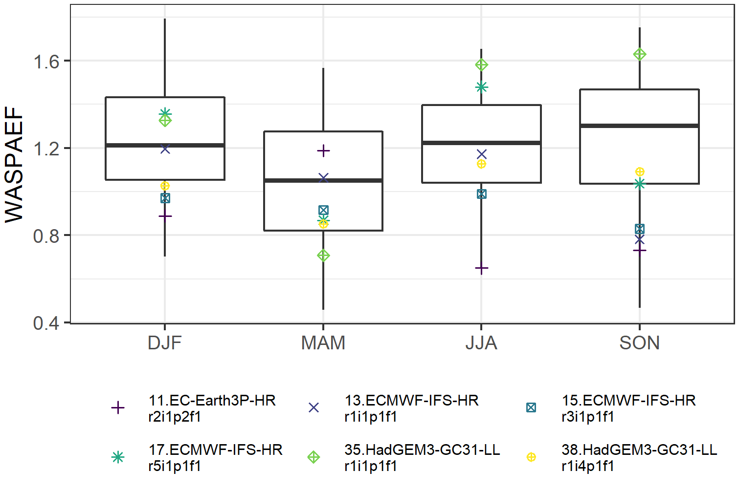
(a) Niño 1.2

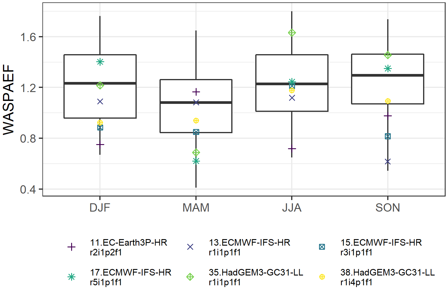
(b) Niño 3

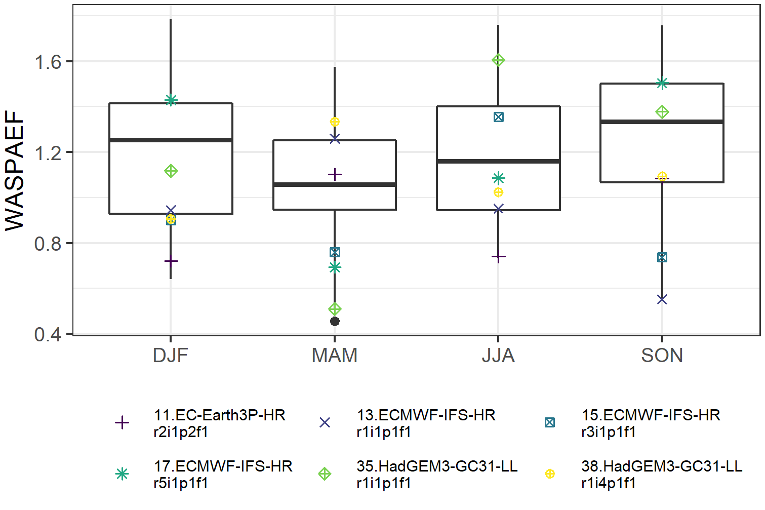
(c) Niño 3.4

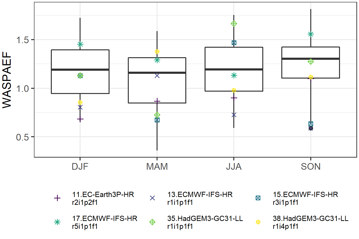
(d) Niño 4

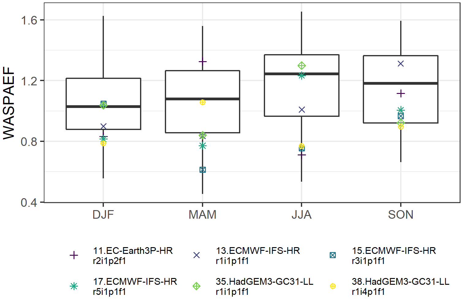
(e) TNA

Figure 10: Teleconnection WSPAEF by season

4 Conclusions

Methods for evaluating model performance are necessary in the atmospheric sciences, where multiple models are constructed to reproduce a climatic variable, and it is important to identify the ones that resemble the reference data. The qualifier “best” can be ambiguous, so defining a “good model” is fundamental, as is determining whether these methods can detect its characteristics.

In this research, it was assumed that a good model is one that generates a field with a high linear correlation with a reference field, as well as similar values for mean, dispersion, and distribution shape. The behavior of six techniques was examined across various scenarios involving these attributes, with three of them being novel in the literature for this particular application. Among these techniques, the WSPAEF, a multi-component measure, demonstrated the highest proficiency in accurately identifying the best alternatives.

A list of 48 CMIP6 models was evaluated with this indicator, based on their ability to reproduce the annual cycle of mean and standard deviation of precipitation and temperature in Central America during the last two decades of the 20th century, as well as the teleconnection patterns in various ENSO and TNA regions. Six models were selected based on three multi-criteria methods. These are: EC-Earth3P-HR (r2i1p2f1), ECMWF-IFS-HR (r1i1p1f1), ECMWF-IFS-HR (r3i1p1f1), ECMWF-IFS-HR (r5i1p1f1), HadGEM3-GC31-LL (r1i1p1f1), HadGEM3-GC31-LL (r1i4p1f1).

When analyzing them individually by variable and month or season, it was identified that their performance is not uniform. For example, the best-performing model overall (EC-Earth3P-HR r2i1p2f1) exhibits poor performance in reproducing the standard deviation of precipitation or the teleconnection patterns during the period from March to May. These performance differences between variables or time periods lead to considering the use of an ensemble of models [46]. The task of reducing the size and precision of these ensembles can be performed using the procedure proposed in this study.

Despite the fact that more intricate methods based on Functional Data Analysis (FDA) did not yield satisfactory outcomes in this study, it is not reasonable to discard this approach. The quest for a metric or procedure enabling a more direct quantification of similarity, devoid of the necessity to aggregate data using statistics like mean and standard deviation, as well as the pursuit of more sophisticated statistical techniques to assess relationships between distinct regions (teleconnections), persist as open challenges.

In addition to introducing the proposed measure and selection method, this work also sheds light on the limitations of other well-established techniques. By doing so, it aims to stimulate the development of new evaluation methods specifically designed for these indicators.

Data availability

The reference data is available at https://psl.noaa.gov/data/gridded/tables/surface.html while the models data can be found at https://esgf-node.llnl.gov/search/cmip6/.

Funding

Not applicable

Conflict of interest

The authors declare no conflict of interest.

Ethics approval

Not applicable

Patient consent

Not applicable

Permission to reproduce material from other sources

Not applicable

Clinical trial registration

Not applicable

Supporting Information

References

- [1] Geophysical Fluid Dynamics Laboratory “Climate Modeling”, 2020 URL: https://www.gfdl.noaa.gov/climate-modeling/
- [2] Joel Katzav and Wendy S. Parker “The future of climate modeling” In Climatic Change 132.4, 2015, pp. 475–487 DOI: 10.1007/s10584-015-1435-x
- [3] Phu Nguyen et al. “Evaluation of CMIP5 Model Precipitation Using PERSIANN-CDR” In Journal of Hydrometeorology 18.9 Boston MA, USA: American Meteorological Society, 2017, pp. 2313–2330 DOI: 10.1175/JHM-D-16-0201.1
- [4] Intergovernmental Panel Climate Change “Evaluation of Climate Models” In Climate Change 2013 – The Physical Science Basis: Working Group I Contribution to the Fifth Assessment Report of the Intergovernmental Panel on Climate Change Cambridge University Press, 2014, pp. 741–866 DOI: 10.1017/CBO9781107415324.020
- [5] Robert Pincus et al. “Evaluating the present-day simulation of clouds, precipitation, and radiation in climate models” In Journal of Geophysical Research: Atmospheres 113.D14, 2008 DOI: https://doi.org/10.1029/2007JD009334
- [6] K.. Raju and Nagesh K.D. “Ranking of global climate models for India using multicriterion analysis” In Climate Research 60.2, 2014, pp. 103–117 URL: https://www.int-res.com/abstracts/cr/v60/n2/p103-117/
- [7] P.. Gleckler, K.. Taylor and C. Doutriaux “Performance metrics for climate models” In Journal of Geophysical Research: Atmospheres 113.D6, 2008 URL: https://agupubs.onlinelibrary.wiley.com/doi/abs/10.1029/2007JD008972
- [8] Reto Knutti “The end of model democracy?” In Climatic Change 102.3, 2010, pp. 395–404 URL: https://doi.org/10.1007/s10584-010-9800-2
- [9] Karl E. Taylor “Summarizing multiple aspects of model performance in a single diagram” In Journal of Geophysical Research: Atmospheres 106.7, 2001, pp. 7183–7192 URL: https://agupubs.onlinelibrary.wiley.com/doi/abs/10.1029/2000JD900719
- [10] M.. Demirel et al. “Combining satellite data and appropriate objective functions for improved spatial pattern performance of a distributed hydrologic model” In Hydrology and Earth System Sciences 22.2, 2018, pp. 1299–1315 DOI: 10.5194/hess-22-1299-2018
- [11] Chengguo Tan and Suiyu Yan “Spatiotemporal data organization and application research” In The International Archives of the Photogrammetry, Remote Sensing and Spatial Information Sciences 42.2, 2017, pp. 1363–1366 URL: https://doaj.org/article/b52c28323dec4e118ba78364aade3fe9
- [12] Christopher K. Wikle, Andrew Zammit-Mangion and Noel Cressie “Spatio-Temporal Statistics with R”, Springer Series in Statistics ChapmanHall/CRC, 2019 URL: https://doi.org/10.1201/9781351769723
- [13] James Ramsay “When the data are functions” In Psychometrika 47, 1982, pp. 379–396 URL: https://doi.org/10.1007/BF02293704
- [14] Jamaludin Suhaila and Zulkifli Yusop “Spatial and temporal variabilities of rainfall data using functional data analysis” In Theoretical and Applied Climatology 129.1, 2017, pp. 229–242 URL: https://doi.org/10.1007/s00704-016-1778-x
- [15] V. Eyring et al. “Overview of the Coupled Model Intercomparison Project Phase 6 (CMIP6) experimental design and organization” In Geoscientific Model Development 9, 2016, pp. 1937–1958 URL: https://doi.org/10.5194/gmd-9-1937-2016
- [16] Allan H. Murphy “Skill Scores Based on the Mean Square Error and Their Relationships to the Correlation Coefficient” In Monthly Weather Review 116.12, 1988, pp. 2417–2424 URL: https://doi.org/10.1175/1520-0493(1988)116%3C2417:SSBOTM%3E2.0.CO;2
- [17] Hugo G. Hidalgo and Eric J. Alfaro “Global Model selection for evaluation of climate change projections in the Eastern Tropical Pacific Seascape” In Revista de Biología Tropical 60.3, 2012, pp. 67–81 URL: http://revistas.ucr.ac.cr/index.php/rbt/issue/archive
- [18] Hugo G. Hidalgo and Eric J. Alfaro “Skill of CMIP5 climate models in reproducing 20th century basic climate features in Central America” In International Journal of Climatology 35.12, 2015, pp. 3397–3421 URL: https://rmets.onlinelibrary.wiley.com/doi/abs/10.1002/joc.4216
- [19] Hoshin V. Gupta, Harald Kling, Koray K. Yilmaz and Guillermo F. Martinez “Decomposition of the mean squared error and NSE performance criteria: Implications for improving hydrological modelling” In Journal of Hydrology 377.1, 2009, pp. 80–91 DOI: https://doi.org/10.1016/j.jhydrol.2009.08.003
- [20] Abel Centella-Artola et al. “Evaluation of Sixteen Gridded Precipitation Datasets over the Caribbean Region Using Gauge Observations” In Atmosphere 11.12, 2020 DOI: 10.3390/atmos11121334
- [21] Michael J. Swain and Dana H. Ballard “Color indexing” In International Journal of Computer Vision 7.1, 1991, pp. 11–32 DOI: 10.1007/BF00130487
- [22] K. Ahmed et al. “Selection of multi-model ensemble of general circulation models for the simulation of precipitation and maximum and minimum temperature based on spatial assessment metrics” In Hydrology and Earth System Sciences 23.11, 2019, pp. 4803–4824 DOI: 10.5194/hess-23-4803-2019
- [23] Cédric Villani “The Wasserstein distances” In Optimal Transport: Old and New Berlin, Heidelberg: Springer Berlin Heidelberg, 2009, pp. 93–111 DOI: 10.1007/978-3-540-71050-9_6
- [24] Victor M. Panaretos and Yoav Zemel “Statistical Aspects of Wasserstein Distances” In Annual Review of Statistics and Its Application 6.1, 2019, pp. 405–431 DOI: 10.1146/annurev-statistics-030718-104938
- [25] Gabriele Vissio, Valerio Lembo, Valerio Lucarini and Michael Ghil “Evaluating the Performance of Climate Models Based on Wasserstein Distance” e2020GL089385 10.1029/2020GL089385 In Geophysical Research Letters 47.21, 2020, pp. e2020GL089385 DOI: https://doi.org/10.1029/2020GL089385
- [26] Espen Bernton, Pierre E Jacob, Mathieu Gerber and Christian P Robert “On parameter estimation with the Wasserstein distance” In Information and Inference: A Journal of the IMA 8.4, 2019, pp. 657–676 DOI: 10.1093/imaiai/iaz003
- [27] Guoqiang Tang, Martyn P. Clark and Simon Michael Papalexiou “The Use of Serially Complete Station Data to Improve the Temporal Continuity of Gridded Precipitation and Temperature Estimates” In Journal of Hydrometeorology 22.6 Boston MA, USA: American Meteorological Society, 2021, pp. 1553–1568 DOI: https://doi.org/10.1175/JHM-D-20-0313.1
- [28] Harald Kling, Martin Fuchs and Maria Paulin “Runoff conditions in the upper Danube basin under an ensemble of climate change scenarios” In Journal of Hydrology 424-425, 2012, pp. 264–277 DOI: https://doi.org/10.1016/j.jhydrol.2012.01.011
- [29] Trevor Harris et al. “Evaluating Proxy Influence in Assimilated Paleoclimate Reconstructions—Testing the Exchangeability of Two Ensembles of Spatial Processes” In Journal of the American Statistical Association, 2020 URL: https://doi.org/10.1080/01621459.2020.1799810
- [30] J.. Tukey “Mathematics and the picturing of data”, 1975
- [31] Martin Schlather et al. “Analysis, Simulation and Prediction of Multivariate Random Fields with Package RandomFields” In Journal of Statistical Software 63.8, 2015, pp. 1–25 URL: http://www.jstatsoft.org/v63/i08/
- [32] Georgy L Shevlyakov and Hannu Oja “Robust correlation: Theory and applications” John Wiley & Sons, 2016
- [33] Zhuhua Lin and Yingchun Zhou “Ranking of functional data in application to worldwide data analysis” In Environmental and Ecological Statistics 24.4, 2017, pp. 469–484 URL: https://doi.org/10.1007/s10651-017-0384-0
- [34] Robert F. Adler et al. “The Version-2 Global Precipitation Climatology Project (GPCP) Monthly Precipitation Analysis (1979–Present)” In Journal of Hydrometeorology 4.6, 2003, pp. 1147–1167 URL: https://doi.org/10.1175/1525-7541(2003)004%3C1147:TVGPCP%3E2.0.CO;2
- [35] E. Kalnay et al. “The NCEP/NCAR 40-Year Reanalysis Project” In Bulletin of the American Meteorological Society 77.3, 1996, pp. 437–472 URL: https://doi.org/10.1175/1520-0477(1996)077%3C0437:TNYRP%3E2.0.CO;2
- [36] Boyin Huang et al. “NOAA Extended Reconstructed Sea Surface Temperature (ERSST), Version 5” NOAA National Centers for Environmental Information, 2017 URL: https://psl.noaa.gov/data/gridded/data.noaa.ersst.v5.html
- [37] Young-Jou Lai, Ting-Yun Liu and Ching-Lai Hwang “TOPSIS for MODM” Facility Location Models for Distribution Planning In European Journal of Operational Research 76.3, 1994, pp. 486–500 DOI: https://doi.org/10.1016/0377-2217(94)90282-8
- [38] J.P. Brans, Ph. Vincke and B. Mareschal “How to select and how to rank projects: The Promethee method” Mathematical Programming Multiple Criteria Decision Making In European Journal of Operational Research 24.2, 1986, pp. 228–238 DOI: https://doi.org/10.1016/0377-2217(86)90044-5
- [39] Wojciech Salabun, Jaroslaw Watróbski and Andrii Shekhovtsov “Are MCDA Methods Benchmarkable? A Comparative Study of TOPSIS, VIKOR, COPRAS, and PROMETHEE II Methods” In Symmetry 12.9, 2020 URL: https://www.mdpi.com/2073-8994/12/9/1549
- [40] S. Sithara, S.. Pramada and Santosh G. Thampi “Statistical downscaling of sea levels: application of multi-criteria analysis for selection of global climate models” In Environmental Monitoring and Assessment 194.10, 2022, pp. 764 DOI: 10.1007/s10661-022-10449-2
- [41] Ritica Thakur and V.. Manekar “Ranking of CMIP6 based High-resolution Global Climate Models for India using TOPSIS” In ISH Journal of Hydraulic Engineering 0.0 Taylor & Francis, 2022, pp. 1–14 DOI: 10.1080/09715010.2021.2015462
- [42] Reza Zamani and Ronny Berndtsson “Evaluation of CMIP5 models for west and southwest Iran using TOPSIS-based method” In Theoretical and Applied Climatology 137.1, 2019, pp. 533–543 DOI: 10.1007/s00704-018-2616-0
- [43] Tito Maldonado, Eric J. Alfaro and Hugo G. Hidalgo “A review of the main drivers and variability of Central America’s Climate and seasonal forecast systems” In Revista de Biología Tropical 66.1-1, 2018, pp. S153–S175 DOI: https://doi.org/10.15517/rbt.v66i1.33294
- [44] Mansour Almazroui et al. “Projected Changes in Temperature and Precipitation Over the United States, Central America, and the Caribbean in CMIP6 GCMs” In Earth Systems and Environment 5.1, 2021, pp. 1–24 DOI: 10.1007/s41748-021-00199-5
- [45] Meng-Zhuo Zhang, Zhongfeng Xu, Ying Han and Weidong Guo “Evaluation of CMIP6 models toward dynamical downscaling over 14 CORDEX domains” In Climate Dynamics Springer, 2022, pp. 1–15 DOI: https://doi.org/10.1007/s00382-022-06355-5
- [46] Swedish Meteorological and Hydrological Institute “Why use a model ensemble?”, 2016 URL: https://climateinformation.org/data-production-and-tailoring/why-use-a-model-ensemble/