Poles and zeros in non-Hermitian systems: Application to photonics

Abstract

Resonances are essential for understanding the interactions between light and matter in photonic systems. The real frequency response of the non-Hermitian systems depends on the complex-valued resonance frequencies, which are the poles of electromagnetic response functions. The zeros of the response functions are often used for designing devices, since the zeros can be located close to the real axis, where they have significant impact on scattering properties. While methods are available to determine the locations of the poles, there is a lack of appropriate approaches to find the zeros in photonic systems. We present an approach to compute poles and zeros based on contour integration of electromagnetic quantities. This also allows to extract sensitivities with respect to geometrical or other parameters enabling efficient device design. The approach is applied to a topical example in nanophotonics, an illuminated metasurface, where the emergence of reflection zeros due to the underlying resonance poles is explored using residue-based modal expansions. The generality and simplicity of the theory allows straightforward transfer to other areas of physics. We expect that easy access to zeros will enable new computer-aided design methods in photonics and other fields.

I Introduction

In the field of photonics, light-matter interactions can be tuned by exploiting resonance phenomena. Examples include tailoring quantum entanglement with atoms and photons in cavities Raimond et al. (2001), probing single molecules with ultrahigh sensitivity Nie and Emory (1997), and realizing efficient single-photon sources Senellart et al. (2017). While electromagnetic observables are measured at real-valued excitation frequencies, the concept of resonances intrinsically considers the complex frequency plane Lalanne et al. (2018); Dyatlov and Zworski (2019). Resonance frequencies are complex-valued as the systems are non-Hermitian, e.g., due to interaction with the environment Wu et al. (2021). Resonances are natural properties of photonic systems, often featuring highly localized electromagnetic field intensities, and correspond to poles of electromagnetic response functions, such as scattering ($S$) matrix, reflection, or transmission coefficients. Resonances can also serve as a basis for the expansion of the response functions. Although most nanophotonic systems support many resonances, often only a few resonances are sufficient to determine the optical response in the real-valued frequency range of interest Sauvan et al. (2022); Nicolet et al. (2023).

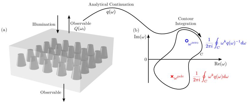
Figure 1: Singularities of physical observables emerge in the complex frequency plane. (a) Schematic of a metasurface illuminated by a plane wave. The response of the nanostructure is typically described by resulting physical observables $Q(\omega_{0})$ for real excitation frequencies $\omega_{0}\in\mathbb{R}$. The corresponding analytical continuation $q(\omega)$ into the complex frequency plane $\omega\in\mathbb{C}$ is considered. (b) Both quantities $q(\omega)$ and $q(\omega)^{-1}$ exhibit singularities in the complex frequency plane. A singularity of $q(\omega)$ is denoted by $\omega^{\mathrm{pole}}$ and a singularity of $q(\omega)^{-1}$ is denoted by $\omega^{\mathrm{zero}}$. There exists a relation between contour integrals involving $q(\omega)$ and $q(\omega)^{-1}$, respectively, and their singularities. This allows for determining the locations of $\omega^{\mathrm{pole}}$ and $\omega^{\mathrm{zero}}$.

Photonic response functions not only have poles but also zeros describing the vanishing of the response functions for the considered input-output channels. Just like the poles in non-Hermitian systems, the zeros generally occur in the complex frequency plane. For example, in systems without absorption, the zeros of the $S$-matrix coefficients are complex conjugates of the underlying poles Nussenzveig (1972). In the case of reflection or transmission coefficients, poles and zeros do not necessarily occur as complex conjugated pairs. In particular, in the absence of absorption, it is possible that zeros lie exactly on the real axis Sweeney et al. (2020); Kang and Genack (2021); Colom et al. (2023). Zeros are equally important for the qualitative prediction of the real frequency response, even if they occur at complex-valued frequencies. Therefore, controlling the relative locations of the poles and zeros in the complex frequency plane can be considered as an alternative, more fundamental approach to design photonic systems in general.

This kind of approach has long been used to design electronic systems Desoer and Schulman (1974). For example, all-pass filters, i.e., systems whose response amplitude remains constant when the excitation frequency is varied, have poles and zeros which are complex conjugates of each other Oppenheim and Verghese (2017). Other examples are minimum-phase systems, where the zeros have to be restricted to the lower part of the complex plane Bechhoefer (2011). In photonic crystals, bound states in the continuum can exist when a pole and a zero of the $S$-matrix coincide on the real axis Hsu et al. (2016). Away from this condition, the pole and zero split and may occur in the complex frequency plane Sakotic et al. (2023). Exceptional points, which have recently attracted much attention in photonics due to their potential for sensing Wiersig (2020), occur when at least two poles or two zeros merge yielding a higher order singularity Miri and Alù (2019); Sweeney et al. (2019); Moritake and Notomi (2023). It has further been shown that a $2\pi$-phase gradient of the reflection or transmission output channel of a metasurface can be realized when a pair of pole and zero is separated by the real axis Colom et al. (2023) and that phase gradient metasurfaces can be designed by exploiting the $2\pi$-phase winding around zeros of cross-polarization reflection coefficients Song et al. (2021). The zeros of photonic systems can have arbitrarily small imaginary parts, i.e., the analysis of the locations of the zeros is extremely relevant to design the response of the systems at real frequencies. Total absorption of light or perfect coherent absorption occurs when zeros of the $S$-matrix are on the real axis Hutley and Maystre (1976); Chong et al. (2010); Maystre (2013). Reflection zeros are also exploited for phase-sensitive detection with nanophotonic cavities in biosensing applications Sreekanth et al. (2018); Kravets et al. (2018).

While in many electronic systems the determination of poles and zeros of the transfer matrix may be done analytically, this is often not possible for photonic structures. To compute zeros of $S$-matrix, reflection, and transmission coefficients of specific systems, it has been proposed to solve Maxwell’s equations as an eigenproblem with appropriately modified boundary conditions Shao et al. (1995); Grigoriev et al. (2013); Bonnet-Ben Dhia et al. (2018); Sweeney et al. (2020).

In this work, we develop a framework for the investigation of poles and zeros of electromagnetic response functions, such as $S$-matrix, reflection, or transmission coefficients, in non-Hermitian systems. The underlying approach exploits a contour integral method well-known in numerical mathematics. The framework, based on scalar physical quantities, extends this approach and enables the simultaneous determination of poles, zeros, sensitivities, and residue-based modal expansions. This is demonstrated by a numerical investigation of the reflection of a photonic metasurface. The occurrence of reflection zeros due to the interference of modal contributions corresponding to poles is observed.

II Singularities and contour integration

In the steady-state regime, light scattering in a material system can be described by the time-harmonic Maxwell’s equation in second-order form,

$$\begin{split}\nabla\times\mu^{-1}&\nabla\times\mathbf{E}-\omega_{0}^{2}\epsilon\mathbf{E}=i\omega_{0}\mathbf{J},\end{split}$$ (1)

where $\mathbf{E}(\mathbf{r},\omega_{0})\in\mathbb{C}^{3}$ is the electric field, $\mathbf{J}(\mathbf{r})\in\mathbb{C}^{3}$ is the electric current density describing a light source, $\epsilon(\mathbf{r},\omega_{0})$ and $\mu(\mathbf{r},\omega_{0})$ are the complex-valued permittivity and permeability tensors, respectively, $\mathbf{r}\in\mathbb{R}^{3}$ is the position, and $\omega_{0}\in\mathbb{R}$ is the angular frequency.

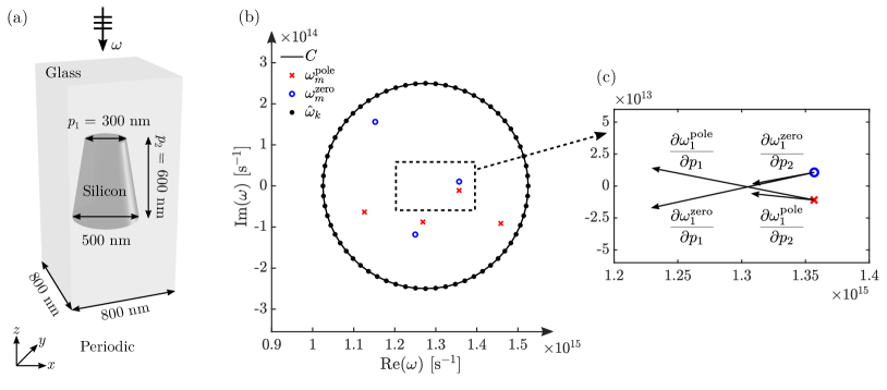
Figure 2: Poles, reflection zeros, and their sensitivities of an illuminated metasurface. (a) Sketch of the unit cell, which is periodic in $x$ and $y$ direction. The metasurface consists of silicon cones with upper radius $p_{1}$ and height $p_{2}$ embedded in an infinitely extended glass medium. The refractive indices of silicon and glass are $n=3.5$ and $n=1.5$, respectively. The illumination is given by a $x$ polarized plane wave of the optical frequency $\omega$ at normal incidence from above. (b) Integration contour $C$, which is a circle with center $1.275\times 10^{15}\,\mathrm{s}^{-1}$ and radius $2.5\times 10^{14}\,\mathrm{s}^{-1}$. The integration contour is numerically discretized by a trapezoidal rule with $64$ integration points $\hat{\omega}_{k}$ marked with black dots. The resulting poles $\omega^{\mathrm{pole}}_{m}$ and reflection zeros $\omega^{\mathrm{zero}}_{m}$ correspond to the Fourier coefficient $q(\omega)$. (c) Detail of the complex frequency plane comprising the two singularities $\omega^{\mathrm{pole}}_{1}$ and $\omega^{\mathrm{zero}}_{1}$. The arrows are associated to the corresponding sensitivities $\partial\omega^{\mathrm{pole}}_{1}/\partial p_{k}$ and $\partial\omega^{\mathrm{zero}}_{1}/\partial p_{k}$ with respect to the shape parameters $p_{1}$ and $p_{2}$. The computation of the sensitivities is also based on integrals along the contour $C$. The complex-valued arrows are given by $\delta\omega=\partial\omega/\partial p\times 100\mathrm{nm}$.

Electromagnetic quantities $Q(\mathbf{E}(\mathbf{r},\omega_{0}))\in\mathbb{C}$ are typically experimentally measured for real excitation frequencies $\omega_{0}\in\mathbb{R}$. However, to obtain deeper insights into light-matter interactions in non-Hermitian systems, an investigation of the optical response for complex frequencies $\omega\in\mathbb{C}$ is essential. For this, we consider the analytical continuation of $Q(\mathbf{E}(\mathbf{r},\omega_{0}))$ into the complex frequency plane, which we denote by $q(\omega)\in\mathbb{C}$ as a short notation of $q(\mathbf{E}(\mathbf{r},\omega))$. Figure 1(a) shows an example from the field of nanophotonics, a dielectric metasurface Mikheeva et al. (2023). Illumination of the metasurface by a plane wave with the optical frequency $\omega_{0}$ yields a physical observable $Q(\omega_{0})$. The singularities of its analytical continuation $q(\omega)$ and the singularities of $q(\omega)^{-1}$ are of special interest and can be used to investigate the properties of the metasurface.

The singularities of $q(\omega)$ are the poles $\omega^{\mathrm{pole}}$ of the physical quantity $q(\omega)$. The associated electric fields are so-called resonances or quasinormal modes, which are also solutions of Eq. (1) without a source term and with losses, e.g., due to open boundaries or dissipation in the system. The singularities of $q(\omega)^{-1}$ are the zeros $\omega^{\mathrm{zero}}$ of $q(\omega)$. The associated electric fields lead to $q(\omega^{\mathrm{zero}})=0$. Figure 1(b) sketches the complex frequency plane with exemplary locations of a pole and a zero. By using Cauchy’s integral theorem for a contour $C$ which encloses one simple pole $\omega^{\mathrm{pole}}$ and (or) one simple zero $\omega^{\mathrm{zero}}$ of the quantity $q(\omega)$, as sketched in Fig. 1(b), $\omega^{\mathrm{pole}}$ and $\omega^{\mathrm{zero}}$ are given by

$$\omega^{\mathrm{pole}}=\frac{\oint\nolimits_{{C}}\omega q(\omega)d\omega}{\oint\nolimits_{{C}}q(\omega)d\omega}\hskip 7.11317pt\mathrm{and}\hskip 7.11317pt\omega^{\mathrm{zero}}=\frac{\oint\nolimits_{{C}}\omega q(\omega)^{-1}d\omega}{\oint\nolimits_{{C}}q(\omega)^{-1}d\omega},$$

respectively. The locations of $M$ poles $\omega^{\mathrm{pole}}_{m}$ inside a contour $C$ are given by the eigenvalues $\omega_{m}$ of the generalized eigenproblem Austin et al. (2014)

$$H^{<}X=HX\Omega,$$ (2)

where $\Omega=\mathrm{diag}(\omega_{1},\dots,\omega_{M})$ is a diagonal matrix containing the eigenvalues, the columns of the matrix $X\in\mathbb{C}^{M\times M}$ are the eigenvectors, and

$$H=\begin{bmatrix}s_{0}&\dots&s_{M-1}\\ \vdots&&\vdots\\ s_{M-1}&\dots&s_{2M-2}\end{bmatrix},\,\,\,H^{<}=\begin{bmatrix}s_{1}&\dots&s_{M}\\ \vdots&&\vdots\\ s_{M}&\dots&s_{2M-1}\end{bmatrix}$$

are Hankel matrices with the contour-integral-based elements

$$s_{k}=\frac{1}{2\pi i}\oint\nolimits_{{C}}\omega^{k}q(\omega)d\omega.$$

The zeros $\omega^{\mathrm{zero}}_{m}$ inside the contour are also given in this way, except that the quantity $q(\omega)^{-1}$ is considered for the elements instead of $q(\omega)$. Note that this type of approach has inspired a family of numerical methods to reliably evaluate all zeros and poles in a given bounded domain. The methods are an active area of research in numerical mathematics, where, e.g., numerical stability, error bounds, and adaptive subdivision schemes are investigated Delves and Lyness (1967); Kravanja and Barel (2000); Austin et al. (2014); Chen (2022). In the field of photonics, poles are usually determined by computing the quasinormal modes as electromagnetic vector fields, where, e.g., the Arnoldi Saad (2011); Yan et al. (2018), FEAST Gavin et al. (2018), or Beyn’s Beyn (2012) algorithm is used. This is in contrast to the approach presented in this work, where scalar physical quantities are considered.

To compute poles and zeros, the elements of the Hankel matrices can be approximated by numerical integration Trefethen and Weideman (2014), where the quantity of interest $q(\omega)$ is calculated by computing $\mathbf{E}(\mathbf{r},\omega)$ for complex frequencies on the integration contour $C$. The electric field $\mathbf{E}(\mathbf{r},\omega)$ can be obtained by numerically solving Maxwell’s equation given in Eq. (1). In general, the electric field is not meromorphic everywhere in the complex plane, due to branch cuts and accumulation points Sauvan et al. (2022). For our approach, the electric field must be analytic only in the spectral region of interest, except at the poles to be investigated. The quantity $q(\omega)^{-1}$ is immediately available by inverting the scalar quantity $q(\omega)$. Computing the different contour integrals for each of the elements requires no additional computational effort since the quantity $q(\omega)$ needs to be calculated only once for each of the integration points. The integrands differ only in the weight functions $\omega^{k}$. Information on the numerical realization can be found in Sec. S1 in the Supplemental Material Sup and in Ref. Betz et al. (2021). Further, the data publication Binkowski et al. (2023) contains software for reproducing the results of this work, based on an interface to the finite-element-based Maxwell solver JCMsuite.

Table 1: Computed pole $\omega^{\mathrm{pole}}_{1}$ and zero $\omega^{\mathrm{zero}}_{1}$ in $\mathrm{s}^{-1}$ and their sensitivities $\partial\omega^{\mathrm{pole}}_{1}/\partial p_{k}$ and $\partial\omega^{\mathrm{zero}}_{1}/\partial p_{k}$ in $(\mathrm{s\,nm})^{-1}$. The sensitivities are computed at the parameter reference values shown in Fig. 2(a) using the $64$ integration points on the contour $C$ depicted in Fig. 2(b). The relative error is defined by $\mathrm{err}(\mathrm{Re}(u))=|(\mathrm{Re}(u)-\mathrm{Re}(u_{\mathrm{ref}}))/\mathrm{Re}(u_{\mathrm{ref}})|$, where $u_{\mathrm{ref}}$ is the reference solution computed with $256$ integration points.

$u$	$\mathrm{Re}(u)$	$\mathrm{Im}(u)$	$\mathrm{err}(\mathrm{Re}(u))$	$\mathrm{err}(\mathrm{Im}(u))$
$\omega^{\mathrm{pole}}_{1}$	$1.357\times 10^{15}$	$-1.095\times 10^{13}$	$<10^{-8}$	$3\times 10^{-8}$
$\frac{\partial\omega^{\mathrm{pole}}_{1}}{\partial p_{1}}$	$-1.257\times 10^{12}$	$2.47\times 10^{11}$	$8\times 10^{-5}$	$6\times 10^{-4}$
$\frac{\partial\omega^{\mathrm{pole}}_{1}}{\partial p_{2}}$	$-4.782\times 10^{11}$	$4.9\times 10^{10}$	$7\times 10^{-5}$	$2\times 10^{-3}$
$\omega^{\mathrm{zero}}_{1}$	$1.357\times 10^{15}$	$1.066\times 10^{13}$	$<10^{-8}$	$3\times 10^{-8}$
$\frac{\partial\omega^{\mathrm{zero}}_{1}}{\partial p_{1}}$	$-1.26\times 10^{12}$	$-2.8\times 10^{11}$	$7\times 10^{-4}$	$3\times 10^{-3}$
$\frac{\partial\omega^{\mathrm{zero}}_{1}}{\partial p_{2}}$	$-4.7\times 10^{11}$	$8.8\times 10^{10}$	$2\times 10^{-3}$	$2\times 10^{-3}$

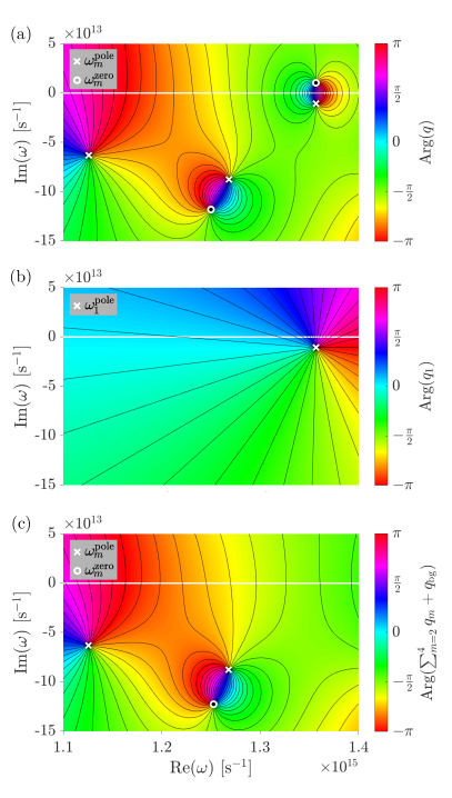
Figure 3: Phase distribution of the electric field reflected from an illuminated metasurface and corresponding modal contributions. (a) Phase $\mathrm{Arg}(q(\omega))$ of the Fourier coefficient $q(\omega)$ in a region enclosed by the contour $C$ shown in Fig. 2(b). This phase distribution is obtained by a modal expansion where $q(\omega)$ is computed only at the integration points $\hat{\omega}_{k}$ on the contour $C$. As expected, the locations of the poles $\omega^{\mathrm{pole}}_{m}$ and zeros $\omega^{\mathrm{zero}}_{m}$ from Fig. 2(b), which are marked with white crosses and circles, respectively, coincide with the poles and zeros of the modal expansion $\mathrm{Arg}(q(\omega))$. (b) Modal contribution $\mathrm{Arg}(q_{1}(\omega))$ to the phase. (c) Sum over remaining phase contributions, $\mathrm{Arg}(\sum_{m=2}^{4}q_{m}(\omega)+q_{\mathrm{bg}}(\omega)$).

III Poles and reflection zeros of a metasurface

We apply this approach to determine the poles $\omega^{\mathrm{pole}}_{m}$ and reflection zeros $\omega^{\mathrm{zero}}_{m}$ of the metasurface sketched in Fig. 1(a). Figure 2(a) shows the geometry of the nanostructures forming the metasurface, including the parameters chosen for the numerical simulation. The metasurface is illuminated by a plane wave at normal incidence from above. For the investigation of the reflected electric field, we consider the Fourier transform of $\mathbf{E}(\mathbf{r},\omega_{0})$ Novotny and Hecht (2012). Due to sub-wavelength periodicity, the resulting upward propagating Fourier spectrum consists of only one term, the zero-order diffraction coefficient $Q(\omega_{0})$. Solving the generalized eigenproblem given by Eq. (2) with the analytical continuation $q(\omega)$ of $Q(\omega_{0})$ gives the poles $\omega^{\mathrm{pole}}_{m}$ and the reflection zeros $\omega^{\mathrm{zero}}_{m}$ of the illuminated metasurface. We emphasize that Eq. (2) provides an expression of both poles and reflection zeros and that the numerical implementation does not pose any difficulties. Figure 2(b) shows the integration contour $C$ and the computed poles and zeros.

The contour-integral-based elements of the Hankel matrices in Eq. (2) allow to apply the approach of direct differentiation Binkowski et al. (2022). When the Fourier coefficients $q(\hat{\omega}_{k})$ are calculated at the integration points $\hat{\omega}_{k}$ on the contour $C$, also their sensitivities $\partial q/\partial p$ with respect to geometry, material, or source parameters $p$ can be evaluated without significant additional computational effort. The sensitivities of the zeros can be extracted in the same way as the sensitivities of the poles can be extracted Binkowski et al. (2022). Figure 2(c) sketches the sensitivities $\partial\omega^{\mathrm{pole}}_{1}/\partial p_{k}$ and $\partial\omega^{\mathrm{zero}}_{1}/\partial p_{k}$ with respect to the upper radius $p_{1}$ and the height $p_{2}$ of the silicon cones of the metasurface. With $64$ integration points, it is possible to compute poles, zeros, and their sensitivities with high accuracies, see Table 1. Numerical convergence with respect to the number of integration points can be observed, see Sec. S1 in the Supplemental Material Sup . To demonstrate the general applicability of the presented approach, we investigate another electromagnetic response function, the transmission coefficients of a photonic structure supporting a bound state in the continuum, in Sec. S2 in the Supplemental Material Sup .

IV Modal expansion in the complex frequency plane

The residues

$$a_{m}=\frac{1}{2\pi i}\oint_{C_{m}}q(\omega)d\omega,$$

where $C_{m}$ are contours enclosing the single eigenvalues $\omega_{m}$ from Eq. (2), can be used as a selection criterion for meaningful eigenvalues $\omega_{m}$. Eigenvalues with large $a_{m}$ are prioritized, while $\omega_{m}$ with small $a_{m}$ are likely to be unphysical eigenvalues because either $M$ is chosen larger than the actual number of eigenvalues within the contour or they are not significant with respect to the quantity of interest. Correspondingly, the choice of a specific source in Eq. (1) allows to regard only a subset of eigenvalues of the considered physical system Betz et al. (2021); Binkowski et al. (2023). Note that, for simple eigenvalues, the residues are directly available, given by $\mathrm{diag}(a_{1},\dots,a_{M})=X^{T}HX$, where $X$ is suitably scaled Binkowski et al. (2023).

Moreover, with the poles $\omega^{\mathrm{pole}}_{m}$ and the corresponding residues $a_{m}$, the residue-based modal expansion of the Fourier coefficient,

$$\begin{split}&q(\omega)=\sum_{m=1}^{M}q_{m}(\omega)+q_{\mathrm{bg}}(\omega),\\ q_{m}(\omega)=&\frac{-a_{m}}{\omega^{\mathrm{pole}}_{m}-\omega},\,\,\,q_{\mathrm{bg}}(\omega)=\frac{1}{2\pi i}\oint_{C}\frac{q(\xi)}{\xi-\omega}d\xi,\end{split}$$ (3)

can be performed, where $q_{m}(\omega)$ are Riesz-projection-based modal contributions and $q_{\mathrm{bg}}(\omega)$ is the background contribution Zschiedrich et al. (2018).

Figure 3(a) shows the phase distribution $\mathrm{Arg}(q(\omega))$ of the electric field reflected from the metasurface shown in Fig. 2(a). This is obtained by evaluating the modal expansion given by Eq. (3) for the contour $C$ shown in Fig. 2(b). A phase retardation of $2\pi$ for a real frequency scan, which is often required for the design of metasurfaces, is obtained when a pair of pole $\omega^{\mathrm{pole}}_{m}$ and zero $\omega^{\mathrm{zero}}_{m}$ is separated by the real axis Colom et al. (2023). Figure 3(b) shows $\mathrm{Arg}(q_{1}(\omega))$ corresponding to the pole $\omega^{\mathrm{pole}}_{1}$ and Fig. 3(c) shows $\mathrm{Arg}(\sum_{m=2}^{4}q_{m}(\omega)+q_{\mathrm{bg}}(\omega))$. In particular, it can be observed that the zero $\omega^{\mathrm{zero}}_{1}$ does not appear for the modal contribution $q_{1}(\omega)$, but it emerges due to interference with the other contributions, i.e., when $\sum_{m=2}^{4}q_{m}(\omega)+q_{\mathrm{bg}}(\omega)$ is added to $q_{1}(\omega)$.

V Conclusion

We presented a theoretical formulation to determine the locations of complex-valued singularities, including poles and zeros, in non-Hermitian systems. The zeros can be determined by contour integration, in the same way as the poles corresponding to resonances can be computed. We also presented residue-based modal expansions in the complex frequency plane of the phase of the field reflected from a photonic metasurface, where the total expansion validated the computed reflection zeros. The different modal contributions give insight into the emergence of the reflection zeros by interference of various expansion terms. Furthermore, computation of partial derivatives of the reflection zeros was demonstrated. The approach can easily be transferred to other physical systems supporting resonances, e.g., to quantum mechanics and acoustics.

The theory essentially relies on detecting singularities of meromorphic functions in the complex plane. Therefore, it can be easily applied to compute other response functions, e.g., $S$-matrix and transmission coefficients, coefficients of the Jones matrix, scattering cross sections of isolated particles, or maximal chiral response of nanoassemblies. The real frequency response of metasurfaces can in many cases be significantly impacted by reflection and transmission zeros, since these typically lie close to the real axis or can even cross the real axis with slight parameter variations, see also Sec. S3 in the Supplemental Material Sup . Therefore, a precise quantification of the sensitivities of reflection and transmission zeros or also of other physical quantities is essential for gradient-based optimization of photonic metasurfaces or other non-Hermitian systems. We expect that the presented theory will enable new computer-aided design approaches.

Data and code availability

Supplementary data tables and source code for the numerical experiments for this work can be found in the open access data publication Binkowski et al. (2023).

See pages 1 of supplement.pdf

See pages 2 of supplement.pdf

See pages 3 of supplement.pdf

See pages 4 of supplement.pdf

See pages 5 of supplement.pdf

See pages 6 of supplement.pdf

References

- Raimond et al. (2001) J. M. Raimond, M. Brune, and S. Haroche, Rev. Mod. Phys. 73, 565 (2001).
- Nie and Emory (1997) S. Nie and S. R. Emory, Science 275, 1102 (1997).
- Senellart et al. (2017) P. Senellart, G. Solomon, and A. White, Nat. Nanotechnol. 12, 1026 (2017).
- Lalanne et al. (2018) P. Lalanne, W. Yan, K. Vynck, C. Sauvan, and J.-P. Hugonin, Laser Photonics Rev. 12, 1700113 (2018).
- Dyatlov and Zworski (2019) S. Dyatlov and M. Zworski, Mathematical theory of scattering resonances (American Mathematical Society, Providence, Rhode Island, 2019).
- Wu et al. (2021) T. Wu, M. Gurioli, and P. Lalanne, ACS Photonics 8, 1522 (2021).
- Sauvan et al. (2022) C. Sauvan, T. Wu, R. Zarouf, E. A. Muljarov, and P. Lalanne, Opt. Express 30, 6846 (2022).
- Nicolet et al. (2023) A. Nicolet, G. Demésy, F. Zolla, C. Campos, J. E. Roman, and C. Geuzaine, Eur. J. Mech. A Solids 100, 104809 (2023).
- Nussenzveig (1972) H. M. Nussenzveig, Causality and dispersion relations (Academic Press, 1972).
- Sweeney et al. (2020) W. R. Sweeney, C. W. Hsu, and A. D. Stone, Phys. Rev. A 102, 063511 (2020).
- Kang and Genack (2021) Y. Kang and A. Z. Genack, Phys. Rev. B 103, L100201 (2021).
- Colom et al. (2023) R. Colom, E. Mikheeva, K. Achouri, J. Zuniga-Perez, N. Bonod, O. J. F. Martin, S. Burger, and P. Genevet, Laser Photonics Rev. 17, 2200976 (2023).
- Desoer and Schulman (1974) C. Desoer and J. Schulman, IEEE Trans. Circuits Syst. 21, 3 (1974).
- Oppenheim and Verghese (2017) A. Oppenheim and G. Verghese, Signals, Systems and Inference, Global Edition (Pearson, 2017).
- Bechhoefer (2011) J. Bechhoefer, Am. J. Phys. 79, 1053 (2011).
- Hsu et al. (2016) C. W. Hsu, B. Zhen, A. D. Stone, J. D. Joannopoulos, and M. Soljačić, Nat. Rev. Mater. 1, 16048 (2016).
- Sakotic et al. (2023) Z. Sakotic, P. Stankovic, V. Bengin, A. Krasnok, A. Alù, and N. Jankovic, Laser Photonics Rev. 17, 2200308 (2023).
- Wiersig (2020) J. Wiersig, Photon. Res. 8, 1457 (2020).
- Miri and Alù (2019) M.-A. Miri and A. Alù, Science 363, eaar7709 (2019).
- Sweeney et al. (2019) W. R. Sweeney, C. W. Hsu, S. Rotter, and A. D. Stone, Phys. Rev. Lett. 122, 093901 (2019).
- Moritake and Notomi (2023) Y. Moritake and M. Notomi, ACS Photonics 10, 667 (2023).
- Song et al. (2021) Q. Song, M. Odeh, J. Zúñiga-Pérez, B. Kanté, and P. Genevet, Science 373, 1133 (2021).
- Hutley and Maystre (1976) M. Hutley and D. Maystre, Opt. Commun. 19, 431 (1976).
- Chong et al. (2010) Y. D. Chong, L. Ge, H. Cao, and A. D. Stone, Phys. Rev. Lett. 105, 053901 (2010).
- Maystre (2013) D. Maystre, C. R. Phys. 14, 381 (2013).
- Sreekanth et al. (2018) K. V. Sreekanth, S. Sreejith, S. Han, A. Mishra, X. Chen, H. Sun, C. T. Lim, and R. Singh, Nat. Commun. 9, 369 (2018).
- Kravets et al. (2018) V. G. Kravets, A. V. Kabashin, W. L. Barnes, and A. N. Grigorenko, Chem. Rev. 118, 5912 (2018).
- Shao et al. (1995) Z. Shao, W. Porod, C. S. Lent, and D. J. Kirkner, J. Appl. Phys. 78, 2177 (1995).
- Grigoriev et al. (2013) V. Grigoriev, A. Tahri, S. Varault, B. Rolly, B. Stout, J. Wenger, and N. Bonod, Phys. Rev. A 88, 011803(R) (2013).
- Bonnet-Ben Dhia et al. (2018) A.-S. Bonnet-Ben Dhia, L. Chesnel, and V. Pagneux, Proc. R. Soc. A 474, 20180050 (2018).
- Mikheeva et al. (2023) E. Mikheeva, R. Colom, K. Achouri, A. Overvig, F. Binkowski, J.-Y. Duboz, S. Cueff, S. Fan, S. Burger, A. Alù, and P. Genevet, Optica 10, 1287 (2023).
- Austin et al. (2014) A. P. Austin, P. Kravanja, and L. N. Trefethen, SIAM J. Numer. Anal. 52, 1795 (2014).
- Delves and Lyness (1967) L. M. Delves and J. N. Lyness, Math. Comp. 21, 543 (1967).
- Kravanja and Barel (2000) P. Kravanja and M. V. Barel, Computing the Zeros of Analytic Functions, Lect. Notes Math. 1727 (Springer, New York, 2000).
- Chen (2022) H. Chen, J. Comput. Appl. Math. 402, 113796 (2022).
- Saad (2011) Y. Saad, Numerical Methods for Large Eigenvalue Problems, 2nd ed. (SIAM, Philadelphia, 2011).
- Yan et al. (2018) W. Yan, R. Faggiani, and P. Lalanne, Phys. Rev. B 97, 205422 (2018).
- Gavin et al. (2018) B. Gavin, A. Miedlar, and E. Polizzi, J. Comput. Sci. 27, 107 (2018).
- Beyn (2012) W.-J. Beyn, Linear Algebra Its Appl. 436, 3839 (2012).
- Trefethen and Weideman (2014) L. N. Trefethen and J. Weideman, SIAM Rev. 56, 385 (2014).
- (41) See Supplemental Material for numerical convergence studies for the investigated metasurface, an examination of poles and transmission zeros of an additional photonic example supporting a bound state in the continuum, and details on using poles and zeros for designing photonic structures, which includes the Refs. Pomplun et al. (2007); Binkowski et al. (2023); Saad (2011); Betz et al. (2021); Koshelev et al. (2018); Hsu et al. (2016); Sakotic et al. (2023); Miri and Alù (2019); Hutley and Maystre (1976); Chong et al. (2010); Sweeney et al. (2020); Mikheeva et al. (2023); Kang and Genack (2021); Colom et al. (2023); Song et al. (2021); Baek et al. (2023); Sweeney et al. (2019); Wang et al. (2021); Ferise et al. (2022); Elsawy et al. (2023).
- Betz et al. (2021) F. Betz, F. Binkowski, and S. Burger, SoftwareX 15, 100763 (2021).
- Binkowski et al. (2023) F. Binkowski, F. Betz, R. Colom, P. Genevet, and S. Burger, “Source code and simulation results: Poles and zeros of electromagnetic quantities in photonic systems,” Zenodo (2023), doi: 10.5281/zenodo.8063932.
- Novotny and Hecht (2012) L. Novotny and B. Hecht, Principles of Nano-Optics, 2nd ed. (Cambridge University Press, Cambridge, 2012).
- Binkowski et al. (2022) F. Binkowski, F. Betz, M. Hammerschmidt, P.-I. Schneider, L. Zschiedrich, and S. Burger, Commun. Phys. 5, 202 (2022).
- Zschiedrich et al. (2018) L. Zschiedrich, F. Binkowski, N. Nikolay, O. Benson, G. Kewes, and S. Burger, Phys. Rev. A 98, 043806 (2018).
- Pomplun et al. (2007) J. Pomplun, S. Burger, L. Zschiedrich, and F. Schmidt, Phys. Status Solidi B 244, 3419 (2007).
- Koshelev et al. (2018) K. Koshelev, S. Lepeshov, M. Liu, A. Bogdanov, and Y. Kivshar, Phys. Rev. Lett. 121, 193903 (2018).
- Baek et al. (2023) S. Baek, S. H. Park, D. Oh, K. Lee, S. Lee, H. Lim, T. Ha, H. S. Park, S. Zhang, L. Yang, et al., Light Sci. Appl. 12, 87 (2023).
- Wang et al. (2021) C. Wang, W. R. Sweeney, A. D. Stone, and L. Yang, Science 373, 1261 (2021).
- Ferise et al. (2022) C. Ferise, P. del Hougne, S. Félix, V. Pagneux, and M. Davy, Phys. Rev. Lett. 128, 203904 (2022).
- Elsawy et al. (2023) M. Elsawy, C. Kyrou, E. Mikheeva, R. Colom, J.-Y. Duboz, K. Z. Kamali, S. Lanteri, D. Neshev, and P. Genevet, Laser Photonics Rev. 17, 2200880 (2023).