Joint Salient Object Detection and Camouflaged Object Detection via Uncertainty-aware Learning

Abstract

Salient objects attract human attention and usually stand out clearly from their surroundings. In contrast, camouflaged objects share similar colors or textures with the environment. In this case, salient objects are typically non-camouflaged, and camouflaged objects are usually not salient. Due to this inherent “contradictory” attribute, we introduce an uncertainty-aware learning pipeline to extensively explore the contradictory information of salient object detection (SOD) and camouflaged object detection (COD) via data-level and task-wise contradiction modeling. We first exploit the “dataset correlation” of these two tasks and claim that the easy samples in the COD dataset can serve as hard samples for SOD to improve the robustness of the SOD model. Based on the assumption that these two models should lead to activation maps highlighting different regions of the same input image, we further introduce a “contrastive” module with a joint-task contrastive learning framework to explicitly model the contradictory attributes of these two tasks. Different from conventional intra-task contrastive learning for unsupervised representation learning, our “contrastive” module is designed to model the task-wise correlation, leading to cross-task representation learning. To better understand the two tasks from the perspective of uncertainty, we extensively investigate the uncertainty estimation techniques for modeling the main uncertainties of the two tasks, namely “task uncertainty” (for SOD) and “data uncertainty” (for COD), and aiming to effectively estimate the challenging regions for each task to achieve difficulty-aware learning. Experimental results on benchmark datasets demonstrate that our solution leads to both state-of-the-art performance and informative uncertainty estimation.

1 Introduction

Visual salient object detection (SOD) aims to localize the salient object(s) of the image that attract human attention. The early work of saliency detection mainly relies on human visual priors based handcrafted features [2, 3, 4] to detect high contrast regions. Deep SOD models [5, 6, 7, 8] use deep saliency features instead of handcrafted features to achieve effective global and local context modeling, leading to better performance. In general, existing SOD models [5, 9, 10, 6, 8] focus on two directions: 1) constructing effective saliency decoders [9, 10] that facilitate high/low-level feature aggregation; and 2) designing appropriate loss functions [6, 8] to achieve structure-preserving saliency detection.

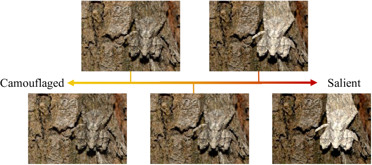
Figure 1: Illustration of the transition from camouflaged objects to salient objects by gradually increasing the contrast of the foreground.

Unlike salient objects that immediately attract human attention, camouflaged objects evolve to blend into their surroundings, effectively avoiding detection by predators. The concept of camouflage has a long history [11], and finds application in various domains including biology [12, 13, 14], military [15, 16, 17] and other fields [18, 19]. From a biological evolution perspective, prey species have developed adaptive mechanisms to camouflage themselves within their environment [20, 21], often by mimicking the structure or texture of their surroundings. These camouflaged objects can only be distinguished by subtle differences. Consequently, camouflaged object detection (COD) models [22, 23, 24, 25, 26] are designed to identify and localize these ”subtle” differences, enabling the comprehensive detection of camouflaged objects.

To address the contradictory nature of SOD and COD, we propose a joint-task learning framework that explores the relationship between these two tasks. Our investigation reveals an inverse relationship between saliency and camouflage, where a higher level of saliency typically indicates a lower level of camouflage, and vice versa. This oppositeness is clearly demonstrated in Fig. 1, where the object gradually transits from camouflaged to salient as the contrast level increases. Hence, we explore the correlation of SOD and COD from both data-wise and task-wise perspectives.

For data-wise correlation modeling, we re-interpret the data augmentation by defining easy samples from COD as hard samples for SOD. By doing so, we achieve contradiction modeling from the dataset perspective. Fig. 1 illustrates that typical camouflaged objects are never salient, but samples in the middle can be defined as hard samples for SOD. Thus, we achieve context-aware data augmentation by the proposed “data interaction as data augmentation” method. In addition, for COD, we find the performance is sensitive to the size of camouflaged objects. To explain this, we crop the foreground camouflaged objects with different percentages of background, and show their corresponding prediction maps and uncertainty maps in Fig. 3. We observe that the cropping based prediction uncertainty, i.e. variance of multiple predictions, is relatively consistent with region-level detectability of the camouflaged objects, validating that performance of the model can be influenced by the complexity of the background. The foreground-cropping strategy can serve as an effective data augmentation technique and a promising uncertainty generation strategy for COD, which also simulates real-world scenarios that camouflaged objects in the wild may appear in different environments. We have also investigated the foreground cropping strategy for SOD, and observed relatively stable predictions, thus the foreground cropping is only applied to COD training dataset.

Aside from data augmentation, we integrate contrastive learning into our framework to address task-wise contradiction modeling. Conventional contrastive learning typically constructs their positive/negative pairs based on semantic invariance. However, since both SOD and COD are class-agnostic tasks that rely on contrast-based object identification, we adopt a different approach for selecting positive/negative pairs based on region contrast. Specifically, given the same input image and its corresponding detected regions for the two tasks, we define region features with similar contrast as positive pairs, while features with different contrast serve as negative pairs. This contrastive module is designed to cater to class-agnostic tasks and effectively captures the contrast differences between the foreground objects in both tasks.

Additionally, we observe two types of “uncertainty” for SOD and COD, respectively, as depicted in Fig. 2. For SOD, the subjective nature [27, 28, 29] and the prediction uncertainty due to the“majority voting” mechanism in labeling procedure, which we define as “task uncertainty.” On the other hand, in COD, uncertainty arises from the difficulty of accurately annotating camouflaged objects due to their resemblance to the background, which we refer to as “data uncertainty.” To address these uncertainties, as shown in the fifth column of Fig. 2, we extensively investigate uncertainty estimation techniques to achieve two main benefits: (1) a self-explanatory model that is aware of its prediction, with an additional uncertainty map to explain the model’s confidence, and (2) difficulty-aware learning, where the estimated uncertainty map serves as an indicator for pixel-wise difficulty representation, facilitating practical hard negative mining.

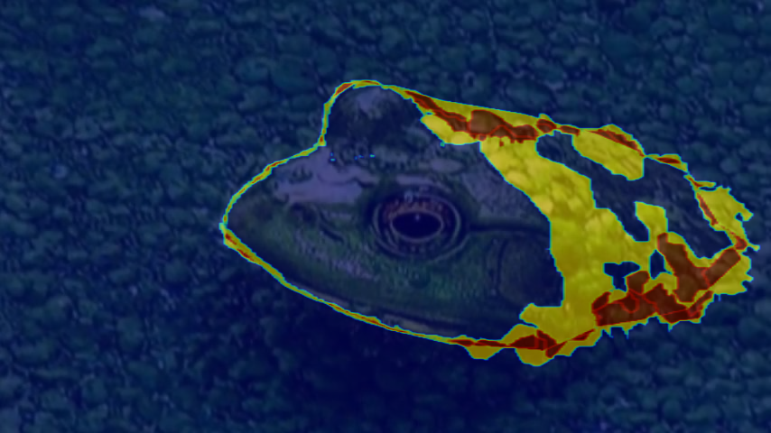
Image	GT	Candidate Annotations		Uncertainty

Figure 2: Inherent uncertainty for SOD ($1^{st}$ row) and COD ($2^{nd}$ row), where the “Candidate Annotations” represent two possible annotations for both tasks, and the “Uncertainty” is the “task uncertainty” ($1^{st}$ row) and “data uncertainty” ($2^{nd}$ row) respectively.

Image	GT	ZoomNet [30]					Ours

Figure 3: Illumination of COD model performance for different percentages of background regions. For each method, from left to right are: image, ground truth, prediction of “CCrop”, “MCrop”, “LCrop”,“Raw” and the uncertainty maps of the four predictions. “CCrop” is achieved via cropping the minimal bounding box that contains the camouflaged objects. “MCrop” and “LCrop” are approximately 65% and 80% of the size of “Raw” image , respectively. Uncertainty maps represent the different predictive regions for the four types of cropped images.

A preliminary version of our work appeared at [1]. Compared with the previous version, we have made the following extensions: 1): We have fully analyzed the relationship between SOD and COD from both dataset and task connection perspectives to further build their relationships. 2): To further investigate the cross-task correlations from the “contrast” perspective, we have introduced contrastive learning to our dual-task learning framework. 3): As an adversarial training based framework, we have investigated more training strategies for the discriminator, leading to more stable training. 4): We have conducted additional experiments to fully explain the task connections, the uncertainty estimation techniques, the experiment setting, and the hyper-parameters.

Our main contributions are summarized as:

• We propose that salient object detection and camouflaged object detection are tasks with opposing attributes for the first time and introduce the first joint learning framework which utilizes category-agnostic “contrastive module” to model the contradictory attributes of two tasks.

• Based on the transitional nature between saliency and camouflage, we introduce “data interaction as data augmentation” by defining simple COD samples as hard SOD samples to achieve context-aware data augmentation for SOD.

• We analyze the main sources of uncertainty in SOD and COD annotations. In order to achieve reliable model predictions, we propose an “uncertainty-aware learning module” as an indicator of model prediction confidence.

• Considering the inherent differences between COD and SOD tasks, we propose “random sampling-based foreground-cropping” as the COD data augmentation technique to simulate the real-world scenarios of camouflaged objects, which significantly improves the performance.

2 Related Work

Salient Object Detection. Existing deep saliency detection models [9, 5, 7, 31, 6, 32, 8] are mainly designed to achieve structure-preserving saliency predictions. [8, 5] introduced an auxiliary edge detection branch to produce a saliency map with precise structure information. Wei et al.  [6] presented structure-aware loss function to penalize prediction along object edges. Wu et al.  [9] designed a cascade partial decoder to achieve accurate saliency detection with finer detailed information. Feng et al.  [32] proposed a boundary-aware mechanism to improve the accuracy of network prediction on the boundary. There also exist salient object detection models that benefit from data of other sources. [33, 34] integrated fixation prediction and salient object detection in a unified framework to explore the connections of the two related tasks. Zeng et al.  [35] presented to jointly learn a weakly supervised semantic segmentation and fully supervised salient object detection model to benefit from both tasks. Zhang et al.  [36] used two refinement structures, combining expanded field of perception and dilated convolution, to increase structural detail without consuming significant computational resources, which are used for salient object detection task on high-resolution images. Liu et al.  [37] designed the stereoscopically attentive multi-scale module to ensure the effectiveness of the lightweight salient object detection model, which uses a soft attention mechanism in any channel at any position, ensuring the presence of multiple scales and reducing the number of parameters.

Camouflaged Object Detection. The concept of camouflage is usually associated with context [38, 39, 40], and the camouflaged object detection models are designed to discover the camouflaged object(s) hidden in the environment. Cuthill et al.  [41] concluded that an effective camouflage includes two mechanisms: background pattern matching, where the color is similar to the environment, and disruptive coloration, which usually involves bright colors along edge, and makes the boundary between camouflaged objects and the background unnoticeable. Bhajantri et al.  [42] utilized co-occurrence matrix to detect defective. Pike et al.  [43] combined several salient visual features to quantify camouflage, which could simulate the visual mechanism of a predator. Le et al.  [23] fused a classification network with a segmentation network and used the classification network to determine the likelihood that the image contains camouflaged objects to produce more accurate camouflaged object detection. In the field of deep learning, Fan et al.  [22] proposed the first publicly available camouflage deep network with the largest camouflaged object training set. Mei et al.  [24] incorporated the predation mechanism of organisms into the camouflaged object detection model and proposed a distraction mining strategy. Zhai et al.  [25] introduced a joint learning model for COD and edge detection based on graph networks, where the two modules simultaneously mine complementary information. Lv et al.  [44] presented a triple-task learning framework to simultaneously rank, localize and segment the camouflaged objects.

Multi-task Learning. The basic assumption of multi-task learning is that there exists shared information among different tasks. In this way, multi-task learning is widely used to extract complementary information about positively related tasks. Kalogeiton et al.  [45] jointly detected objects and actions in a video scene. Zhen et al.  [46] designed a joint semantic segmentation and boundary detection framework by iteratively fusing feature maps generated for each task with a pyramid context module. In order to solve the problem of insufficient supervision in semantic alignment and object landmark detection, Jeon et al.  [47] designed a joint loss function to impose constraints between tasks, and only reliable matched pairs were used to improve the model robustness with weak supervision. Joung et al.  [48] solved the problem of object viewpoint changes in 3D object detection and viewpoint estimation with a cylindrical convolutional network, which obtains view-specific features with structural information at each viewpoint for both two tasks. Luo et al.  [49] presented a multi-task framework for referring expression comprehension and segmentation.

Uncertainty-aware Learning. Difficulty-aware (or uncertainty-aware, confidence-aware) learning aims to explore the contribution of hard samples, leading to hard-negative mining [50], which has been widely used in medical image segmentation [51, 52, 53, 54], semantic segmentation [55, 56, 50], and other fields [57]. To achieve difficulty-aware learning, one needs to estimate model confidence. To achieve this, Gal et al.  [58] used Monte Carlo dropout (MC-Dropout) as a Bayesian approximation, where model uncertainty can be obtained with dropout neural networks. Deep Ensemble [59, 60, 61] is another popular type of uncertainty modeling technique, which usually involves generating an ensemble of predictions to obtain variance of predictions as the uncertainty estimation. With extra latent variable involved, the latent variable models [62, 63, 64] can also be used to achieve predictive distribution estimation, leading to uncertainty modeling. Following the uncertainty-aware learning pipeline, Lin et al.  [50] introduced focal loss to balance the contribution of simple and hard samples for loss updating. Li et al.  [55] presented a deep layer cascade model for semantic segmentation to pay more attention to the difficult parts. Nie et al.  [51] adopted adversarial learning to generate confidence levels for predicting segmentation maps, and then used the generated confidence levels to achieve difficulty-aware learning. Xie et al.  [56] applied difficulty-aware learning to an active learning task, where the difficult samples are claimed to be more informative.

Contrastive learning. The initial goal of contrastive learning [65, 66, 67, 68, 69, 70] is to achieve effective feature representation via self-supervised learning. The main strategy to achieve this is through constructing positive/negative pairs via data augmentation techniques [71, 72, 73, 74, 75, 76, 77, 78], where the basic principle is that similar concepts should have similar representation, thus stay close to each other in the embedding space. On the contrary, dissimilar concepts should stay apart in the embedding space. Different from augmentation based self-supervised contrastive learning, supervised contrastive learning builds the positive/negative pairs based on the given labels [67, 68, 70]. Especially for image segmentation, the widely used loss function is cross-entropy loss. However, it’s well known that cross-entropy loss is not robust to labeling noise [79] and the produced category margins are not separable enough for better generalizing. Further, it penalizes pixel-wise predictions independently without modeling the cross-pixel relationships. Supervised contrastive learning [80] can fix the above issues with robust feature embedding exploration, following the similar training pipeline as self-supervised contrastive learning.

3 Our Method

We propose an uncertainty-aware joint learning framework via contrastive learning (see Fig. 4) to learn SOD and COD in a unified framework. Firstly, we explain that these two tasks are both contradictory and closely related (Sec. 3.1), and a joint learning pipeline can benefit each other with effective context modeling. Then, we present a “Contrastive Module” to explicitly model the “contradicting” attributes of these two tasks (Sec. 3.2), with a data-interaction technique to achieve context-level data augmentation. Further, considering uncertainty for both tasks, we introduce a difficulty-aware learning network (Sec. 3.3) to produce predictions with corresponding uncertainty maps, representing the model’s awareness of the predictions.

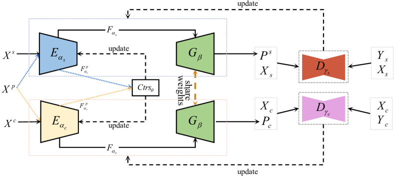
Figure 4: Overview of the proposed uncertainty-aware joint learning network. The “Feature Encoders” for SOD $E_{\alpha_{s}}$ and COD $E_{\alpha_{c}}$ are used to extract independent feature representation $F_{\alpha_{s}}$ and $F_{\alpha_{c}}$, respectively. Given the feature representation of auxiliary image $X^{p}$, the contrastive module $\mathit{Ctrs}_{\theta}$ is presented to model the contradicting attributes of SOD and COD, achieving effective multi-task learning, and based on which the “Prediction Decoders” $G_{\beta}$ share weights to produce fine-grained SOD prediction $P_{s}$ and COD prediction $P_{c}$. As an adversarial learning network, we extract confidence indicators from the two discriminators $D_{\gamma_{s}}$ and $D_{\gamma_{c}}$ for uncertainty-aware learning to distinguish the prediction from the ground truth.

3.1 Tasks Analysis

3.1.1 Tasks Relationship Exploration

Model Perspective: At the task level, both SOD and COD are class-agnostic binary segmentation tasks, where a UNet [81] structure is usually designed to achieve mapping from input (image) space to output (segmentation) space. Differently, the foreground of SOD usually stands out highly from the context, while camouflaged instances are evolved to conceal in the environment. With the above understanding about both SOD and COD, we observe “complementary” information between the two tasks. Given the same image, we claim that due to the “contradicting” attributes of saliency and camouflage, the extracted features for each task should be different from each other, and the localized region of each task should be different as well.

Dataset Perspective: At the dataset level, we observe some samples within the COD dataset can also be included in the SOD dataset (see Fig. 6), where the camouflaged region is consistent with the salient region. However, due to the similar appearance of foreground and background, these samples are easy for COD but challenging for SOD, making them effective for serving as hard samples for SOD to achieve hard negative mining. On the other side, most of the salient foreground in the SOD dataset has high contrast, and the camouflaged regions of the same image usually differ from the salient regions. In this way, samples in the SOD dataset usually cannot serve as simple samples for COD. Considering the dataset relationships of both tasks, we claim that easy samples in the COD dataset can effectively serve as hard samples for SOD to achieve context-level data augmentation.

3.1.2 Inherent Uncertainty

Subjective Nature of SOD: To reflect the human visual system, the initial saliency annotation of each image is obtained with multiple annotators [82, 83, 3, 84], and then “majority voting” is performed to generate the final ground truth saliency map that represents the majority salient regions, e.g. the DUTS dataset [82], ECSSD [83], DUT [3] dataset are annotated by five annotators and HKU-IS [84] is annotated by three annotators. Further, to maintain consistency of the annotated data, some SOD datasets adopt the pre-selection strategy, where the images contain no common salient regions across all the annotators will be removed before the labeling process, e.g. HKU-IS [84] dataset first evaluates the consistency of the annotation of the three annotators, and removes the images with greater disagreement. In the end, 4,447 images are obtained from an initial dataset with 7,320 images. We argue that both the majority voting process for final label generation and the pre-selection process for candidate dataset preparation introduce bias to both the dataset and the models trained on it. We explain this as the “subjective nature” of saliency.

Labeling Uncertainty of COD: Camouflaged objects are evolved to have similar texture and color information to their surroundings [38, 41]. Due to the similar appearance of camouflaged objects and their habitats, it’s more difficult to accurately annotate the camouflaged instance than generic object segmentation, especially along instance boundaries. This poses severe and inevitable labeling noise while generating the camouflaged object detection dataset, which we define as “labeling uncertainty” of camouflage.

3.2 Joint-task Contrastive Learning

As a joint learning framework, we have two sets of training dataset for each individual task, namely a SOD dataset $D_{s}=\{x_{i}^{s},y_{i}^{s}\}_{i=1}^{N_{s}}$ for SOD and a COD dataset $D_{c}=\{x_{i}^{c},y_{i}^{c}\}_{i=1}^{N_{c}}$ for COD, where $\{x_{i}^{s},y_{i}^{s}\}$ is the SOD image/ground truth pair and $\{x_{i}^{c},y_{i}^{c}\}$ is the COD image/ground truth pair, and $i$ indexes images, $N_{s}$ and $N_{c}$ are the size of training dataset for each task. Motivated by both the task contradiction and data sharing attributes of the two tasks, we introduce a contrastive learning based joint-task learning pipeline for joint salient object detection and camouflaged object detection. Firstly, we model the “task contradiction” (Section 3.2.1) with a “contrastive module”. Secondly, we select easy samples by weighted MAE from the COD training dataset (Section 3.2.2), serving as hard samples for SOD.

3.2.1 Task Correlation Modeling via Contrastive Learning

To model the task-wise correlation, we design a “Contrastive Module” in Fig. 4 and introduce another set of images from the PASCAL VOC 2007 dataset [85] as “connection modeling” dataset $D_{p}=\{x_{i}^{p}\}_{i=1}^{N_{p}}$, from which we extract both the camouflaged features and the salient features. With the three datasets (SOD dataset $D_{s}$, COD dataset $D_{c}$ and connection modeling dataset $D_{p}$), our contradicting modeling framework uses the “Feature Encoder” module to extract both the camouflage feature and the saliency feature. The “Prediction Decoder” is then used to produce the prediction of each task. We further present a “Contrastive Module” to model the connection of the two tasks with the connection modeling dataset.

Feature Encoder: The “Feature Encoder” takes the RGB image ($x^{s}$ or $x^{c}$) as input to produce task-specific predictions and also serves as the feature extractor for the “Contrastive Module”. We design both the saliency encoder $E_{\alpha_{s}}$ and camouflage encoder $E_{\alpha_{c}}$ with the same backbone network, e.g. the ResNet50 [86], where $\alpha_{s}$ and $\alpha_{c}$ are the corresponding network parameter sets. The ResNet50 backbone network has four groups of convolutional layers of channel size 256, 512, 1024 and 2048 respectively. We then define the output features of both encoders as $F_{\alpha_{s}}=\{f^{s}_{k}\}_{k=1}^{4}$ and $F_{\alpha_{c}}=\{f^{c}_{k}\}_{k=1}^{4}$, where $k$ indexes the feature group.

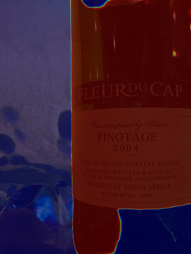
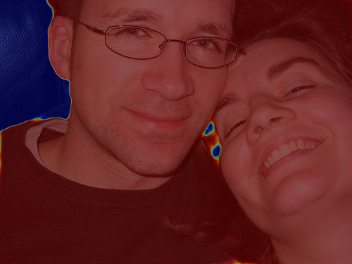
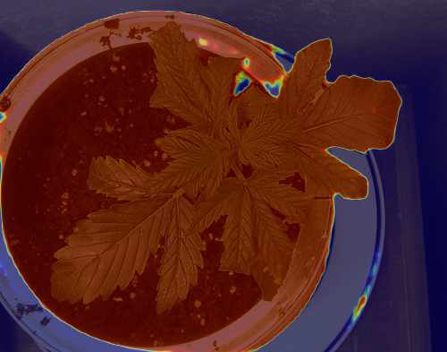
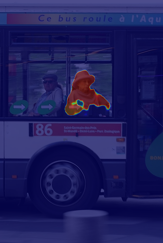
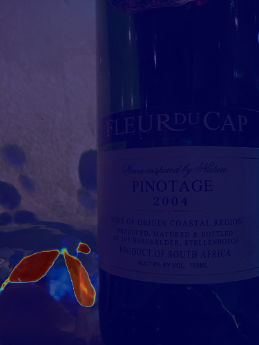
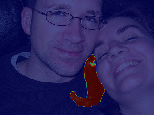
Figure 5: Detected regions from the saliency encoder branch ($1^{st}$ row) and the camouflage encoder branch ($2^{nd}$ row).

Prediction Decoder: As shown in Fig. 4, we design a shared decoder structure for our joint learning framework. To reduce the computational burden, also to achieve feature with larger receptive field, we first attach a multi-scale dilated convolution [87] of output channel size $C=32$ to each backbone feature to generate the new backbone features $F^{\prime}_{\alpha_{s}}=\{f^{cs}_{k}\}_{k=1}^{4}$ and $F^{\prime}_{\alpha_{c}}=\{f^{cc}_{k}\}_{k=1}^{4}$ for each specific task from $F_{\alpha_{s}}$ and $F_{\alpha_{c}}$. Then, we adopt the residual attention based feature fusion strategy from [88] to achieve high/low level feature aggregation. Specifically, the lower-level features are fed to a residual connection module [89] with two $3\times 3$ convolutional layers, which is then added to the higher level feature. The sum of the high/low level feature is then fed to another residual connection block of the same structure as above to generate the fused feature. We perform the above feature fusion operation until we reach the lowest level feature, e.g. $f^{cc}_{1}$ or $f^{cs}_{1}$. To generate the prediction for each task, we design a classifier module, which is composed of three cascaded convolutional layers, where the kernel size of the first two convolutional layers is $3\times 3$, and that of the last convolutional layer is $1\times 1$. After generating initial predictions, we used the holistic attention module [9] for feature optimization to obtain further improved predictions, as the final predictions. To simplify the explanation, we only use prediction after the holistic attention module as the decoder output. We then define prediction of each task as: $G_{\beta}(F_{\alpha_{s}})$ for SOD and $G_{\beta}(F_{\alpha_{c}})$ for COD, where $\beta$ represents the parameter set of the shared prediction decoder.

Contrastive Module: The “Contrastive Module” $\mathit{Ctrs}_{\theta}$ aims to enhance the identity of each task with the feature of other tasks as guidance. Specifically, it takes image $x^{p}$ from the connection modeling dataset $D_{p}=\{x_{i}^{p}\}_{i=1}^{N_{p}}$ as input to model the feature correlation of SOD and COD, where $\theta$ is parameter set of the contrastive module.

For image $x^{p}$ from the connection modeling dataset, its saliency and camouflage features are $F^{p}_{\alpha_{s}}=\{f^{p}_{sk}\}_{k=1}^{4}$ and $F^{p}_{\alpha_{c}}=\{f^{p}_{ck}\}_{k=1}^{4}$, respectively. With the shared decoder $G_{\beta}$, the prediction map are $G_{\beta}(F^{p}_{\alpha_{s}})$ indicating the saliency map and $G_{\beta}(F^{p}_{\alpha_{c}})$ as the camouflage map. The contrastive module decides positive/negative pairs based on contrast information, where regions of similar contrast are defined as positive pairs and the different contrast regions are defined as negative pairs. The intuition behind this is that COD and SOD are both contrast based class-agnostic binary segmentation tasks, making conventional category-aware contrastive learning infeasible to work in this scenario. Considering the goal of building the positive/negative pairs for contrastive learning is to learn representative features via exploring the inherent data correlation, i.e. the category information, we argue the inherent correlation in our scenario is the “contrast” information. For SOD, the foreground shows higher contrast compared with the background, indicating the different contrast level. For COD, the contrast levels of foreground and background are similar. Thus given the same input image $x^{p}$, we decide positive/negative pairs based on the contrast information of the activated regions.

In Fig. 5, we show the activation region (the processed predictions) of the same image from both the saliency encoder (first row) and camouflage encoder (second row). Specifically, given same image $x^{p}$, we compute its camouflage map and saliency map, and highlight the detected foreground region in red. Fig. 5 shows that the two encoders focus on different regions of the image, where the saliency encoder pays more attention to the region that stands out from the context. The camouflage encoder focuses more on the hidden object with similar color or structure as the background, which is consistent with our assumption that these two tasks are contradicting with each other in general.

Feature definition: Following the conventional practice of contrastive learning, our contrastive module $Ctrs_{\theta}$ maps image features, i.e. $F^{p}_{\alpha_{s}}$ and $F^{p}_{\alpha_{c}}$ for the connection modeling data $x^{p}$, to the lower dimensional feature space via four spectral normed convolutional layers (SNconv) [90], which is proven effective in preserving the geometric distance in the compressed space. We then compute saliency and camouflage features of the same image:

$$F^{p}_{sf} =S(G_{\beta}(F^{p}_{\alpha_{s}}),Ctrs_{\theta}(F^{p}_{\alpha_{s}})),$$ (1)

$$F^{p}_{sb} =S((1-G_{\beta}(F^{p}_{\alpha_{s}})),Ctrs_{\theta}(F^{p}_{\alpha_{s}})),$$

$$F^{p}_{\mathit{cf}} =S(G_{\beta}(F^{p}_{\alpha_{c}}),Ctrs_{\theta}(F^{p}_{\alpha_{c}})),$$

$$F^{p}_{cb} =S((1-G_{\beta}(F^{p}_{\alpha_{c}})),Ctrs_{\theta}(F^{p}_{\alpha_{c}})),$$

where $S(\cdot,\cdot)$ computes the region feature via matrix multiplication [91], where the feature maps, i.e. $Ctrs_{\theta}(F^{p}_{\alpha_{s}})$, are scaled to be the same spatial size as the activation map, i.e. $G_{\beta}(F^{p}_{\alpha_{s}})$. $F^{p}_{sf}\in\mathbb{R}^{1\times C}$ and $F^{p}_{sb}\in\mathbb{R}^{1\times C}$ in Eq. (1) represent the SOD foreground and background features, and $F^{p}_{\mathit{cf}}$ and $F^{p}_{cb}$ are the COD foreground and background features, respectively.

Positive/negative pair construction: According to our previous discussion, we define three sets of positive pairs based on contrast similarity: (1) The SOD background feature and COD background feature of the same image should be highly similar, indicating similar contrast information; (2) Due to the nature of the camouflaged object, the foreground and the background features of COD are similar as well as camouflaged object shares similar contrast with the background; (3) Similarly, the COD foreground feature and SOD background feature are also similar in contrast. On the other hand, the negative pair consists of SOD foreground feature and background feature.

Contrastive loss: Given the positive/negative pairs, we follow [92] and define the contrastive loss as:

$$\mathcal{L}_{ctrs}=-\log\frac{\textstyle\sum_{pos}}{{\textstyle\sum_{pos}}+\exp(c(F^{p}_{sf},F^{p}_{sb}))},$$ (2)

where $c(\cdot)$ measures the cosine similarity of the normalized vectors. $\textstyle\sum_{pos}$ represents the similarity of positive pairs, which is defined as:

$${\textstyle\sum_{pos}}=\exp(c(F^{p}_{cf},F^{p}_{cb}))+\exp(c(F^{p}_{sb},F^{p}_{cb}))+\exp(c(F^{p}_{sb},F^{p}_{cf})).$$ (3)

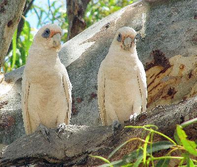
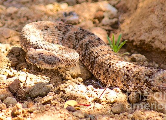
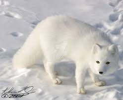
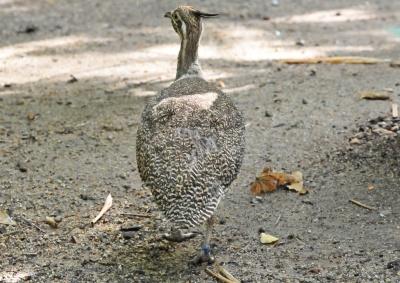
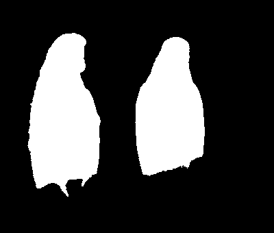
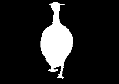
Figure 6: Selected easy samples from the COD training dataset.

3.2.2 Data Interaction

In Section 3.2, we discuss the contradicting modeling strategy to model the two tasks from the model correlation perspective. In this section, we further explore the task relationships from dataset perspective, and introduce data interaction as data augmentation.

Sample selection principle: As shown in Fig. 1, saliency and camouflage are two properties that can transfer from each other. We find that there exist samples in the COD dataset that are both salient and camouflaged. We argue that those samples can be treated as hard samples for SOD to achieve robust learning. The main requirement is that the activation of those samples for SOD and COD should be similar. In other words, the predictions of the selected images for both tasks need to be similar. To select those samples from the COD dataset, we resort to weighted Mean Absolute Error ($\mathit{wMAE}$), and select samples in the COD dataset [22] which achieve the smallest $\mathit{wMAE}$ by testing it using a trained SOD model.

The weighted mean absolute error $\mathit{wMAE}$ is defined as :

$$\mathit{wMAE}=\frac{\sum_{u=1}^{W}\sum_{v=1}^{H}|y^{u,v}-p^{u,v}|}{\sum_{u=1}^{W}\sum_{v=1}^{H}y^{u,v}},$$ (4)

where ${u,v}$ is the pixel index, $p$ represents the model prediction, $y$ is the corresponding ground-truth, and $W$ and $H$ indicate size of $y$. Compared with mean absolute error, $\mathit{wMAE}$ avoids the biased selection caused by different sizes of the foreground object(s).

Data interaction: For the COD training dataset $D_{c}=\{x_{i}^{c},y_{i}^{c}\}_{i=1}^{N_{c}}$ and the trained SOD model $M_{\theta_{s}}$, we obtain saliency prediction of the images in $D_{c}$ as $P^{c}_{s}=M_{\theta_{s}}(\{x^{c}\})=\{p^{c}_{i}\}_{i=1}^{N_{c}}$, where $p_{i}^{c}$ is the saliency prediction of the COD training dataset. We assume that easy samples for COD can be treated as hard samples for SOD as shown in Fig. 1. Then we select $M=403$ samples $D_{c}^{M}$ with the smallest $\mathit{wMAE}$ in $D_{c}$ via Eq. (4), and add in our SOD training dataset [82] as a data augmentation technique. We show the selected samples in Fig. 6, which clearly illustrates the partially positive connection of the two tasks at the dataset level.

3.2.3 Foreground Cropping as Data Augmentation:

Considering the real-life scenarios, camouflaged objects can appear in different sizes, we introduce foreground cropping to achieve context-aware data augmentation. Note that we only perform foreground cropping for COD as the prediction of SOD is relatively stable with different sizes of the foreground object(s). Specifically, we first define the largest bounding box region that covers all the camouflaged objects as the compact cropping (“CCrop”). Then, we obtain the median cropping (“MCrop”) and loose cropping (“LCrop”) by randomly extending $0-80$ and $0-150$ pixels respectively randomly outward along the compact bounding box. We perform cropping on the raw images and resize the cropped image back to the pre-defined training image size for training.

3.3 Uncertainty-aware Learning

In Section 3.1, we discussed that both SOD and COD have inherent uncertainty, where the “subjective nature” of SOD poses serious “model uncertainty” [93] for SOD and difficulty of labeling introduces “data uncertainty” [93] for COD. As shown in Fig. 2, for the SOD dataset, the uncertainty comes from the ambiguity of saliency. For the COD dataset, the uncertainty mainly comes from the difficulty of labeling (the accuracy of $y_{i}$). To model the uncertainty of both tasks for reliable model generation, we introduce an uncertainty-aware adversarial training strategy to model the task-specific uncertainty in our joint learning framework.

Adversarial learning framework: Following the conventional practice of generative adversarial network (GAN) [64], we design a fully convolutional discriminator network to evaluate confidence of the predictions. The fully convolutional discriminator network $D_{\gamma}$ consists of five SNconv layers [90] of kernel size $3\times 3$. As a conditional generation task, the fully convolutional discriminator takes the prediction/ground truth and the conditional variable, i.e. the RGB image, as input, and produces a one-channel confidence map, where $\gamma$ is the network parameter set. Note that we have batch normalization and leaky relu layers after the first four convolutional layers. $D_{\gamma}$ aims to distinguish areas of uncertainty, which produce all-zero output with ground truth $y$ as input, and produce $|p-y|$ output with prediction map $p$ as input.

In our case, the fully convolutional discriminator aims to discover the hard (or uncertain) regions of the input image. We use the same structure of discriminators with parameter sets $\gamma_{s}$ and $\gamma_{c}$ for SOD and COD respectively, to identify the two types of challenging regions, i.e. the “subjective area” for SOD, and the “ambiguous regions” for COD.

Uncertainty-aware learning: For the prediction decoder module, we first have the task-specific loss function to learn each task. Specifically, we adopt the structure-aware loss function [6] for both SOD and COD, and define the loss function as:

$$\mathcal{L}_{str}(p,y)=\omega*\mathcal{L}_{ce}(p,y)+\mathcal{L}_{iou}^{\omega}(p,y),$$ (5)

where $\omega$ is the edge-aware weight, which is defined as $\omega=1+5*\left|(avg\_pool(y)-y)\right|$, $y$ is task-specific ground truth, $\mathcal{L}_{ce}$ is the binary cross-entropy loss, $\mathcal{L}_{iou}^{\omega}$ is the weighted boundary-IOU loss [94]. In this way, the task specific loss functions $\mathcal{L}_{str}^{s}$ and $\mathcal{L}_{str}^{c}$ for SOD and COD are defined as:

$$\mathcal{L}_{str}^{s}=\mathcal{L}_{str}(G_{\beta}(F_{\alpha_{s}}),y^{s}),$$ (6)

$$\mathcal{L}_{str}^{c}=\mathcal{L}_{str}(G_{\beta}(F_{\alpha_{c}}),y^{c}),$$ (7)

To achieve adversarial learning, following [95], we further introduce adversarial loss function to both SOD and COD predictors, which is defined as a consistency loss between discriminators prediction of prediction map and discriminators prediction of ground-truth, aiming to fool the discriminators that the prediction of SOD or COD is the actual ground truth. The adversarial loss functions ($\mathcal{L}_{adv}^{s}$ and $\mathcal{L}_{adv}^{c}$) for SOD and COD, respectively, are defined as:

$$\mathcal{L}_{adv}^{s}=\mathcal{L}_{ce}(D_{\gamma_{s}}(x^{s},G_{\beta}(F_{\alpha_{s}})),D_{\gamma_{s}}(x^{s},y^{s})),$$ (8)

$$\mathcal{L}_{adv}^{c}=\mathcal{L}_{ce}(D_{\gamma_{c}}(x^{c},G_{\beta}(F_{\alpha_{c}})),D_{\gamma_{c}}(x^{c},y^{c})),$$ (9)

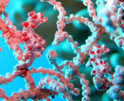
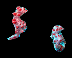
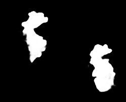
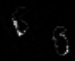
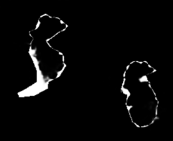
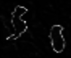
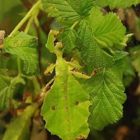
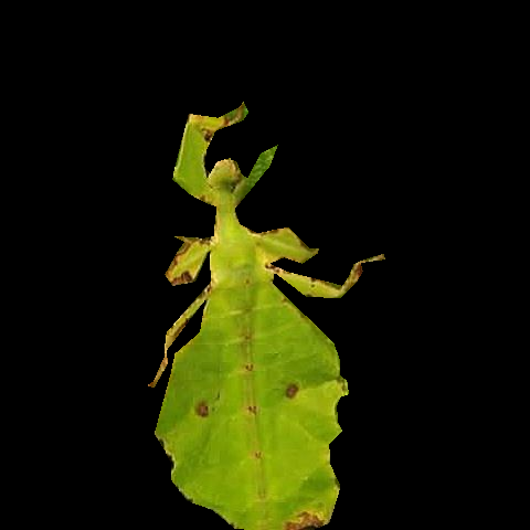
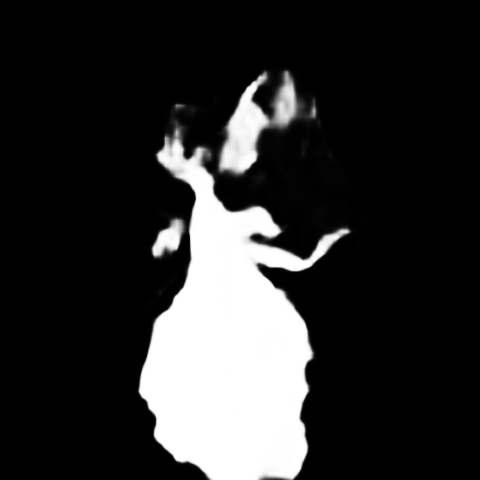
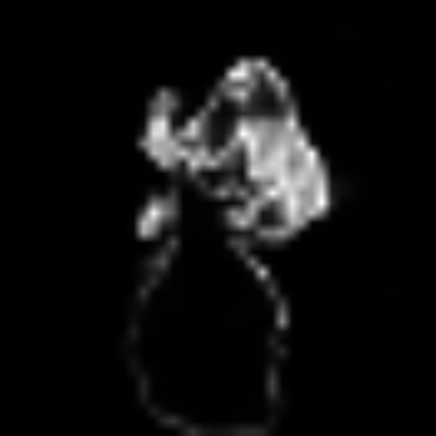
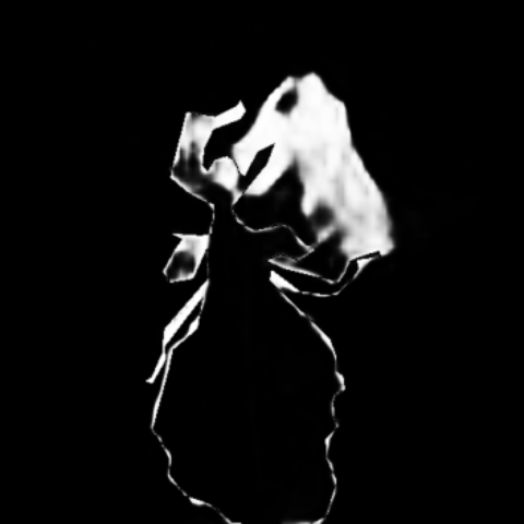
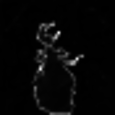
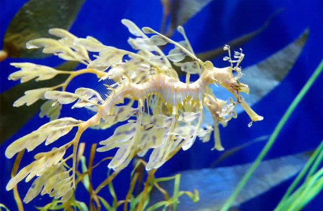
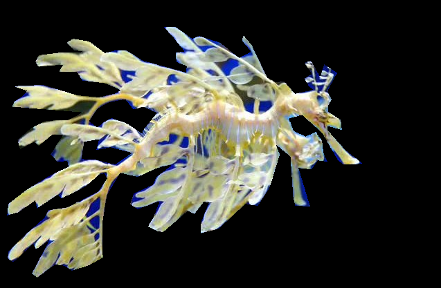
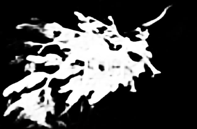
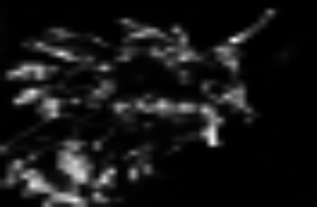
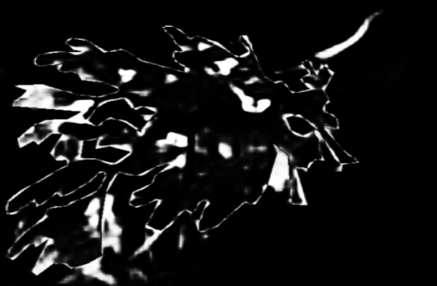
Image	GT	Pred	$D_{\gamma_{s}}(x^{s},G_{\beta}(F_{\alpha_{s}}))$	$|G_{\beta}(F_{\alpha_{s}})-y^{s}|$	$D_{\gamma_{c}}(x^{c},y^{c})$	0

Figure 7: Illumination of the ground truth and predictions of the discriminator, where “Image”, “GT” and “Pred” are the RGB image, the camouflage ground truth map, and the camouflage prediction. The definition of other items is defined in Eq. (10) and Eq. (11). The discriminator is designed to highlight the error predictions, leading to ground-truth aware uncertainty generation at the testing stage.

Both the task specific loss in Eq. (6), Eq. (7) and the adversarial loss in Eq. (8), Eq. (9) are used to update the task-specific network (the generator). To update the discriminator, following the conventional GAN, we want it to distinguish areas of uncertainty clearly. Due to the inherent uncertainty that cannot be directly described, the uncertainty in inputting the ground truth cannot be accurately represented. However, because the correctly annotated regions are dominant in the complete dataset, we believe that the network can perceive the areas that are difficult to learn. The adversarial learning mechanism makes it difficult for the discriminator to distinguish between predicted and ground truth maps, and it can differentiate between noisy ground truth images and areas where RGB images cannot be aligned. Therefore, the output of the discriminator when inputting ground truth is defined as an all-zero map. Additionally, it produces a residual output for the prediction map. The outputs corresponding to different inputs of the discriminator are shown in Fig. 7. Then, the discriminators ($D_{\gamma_{s}}$ and $D_{\gamma_{c}}$) are updated via:

$$\mathcal{L}_{dis}^{s}=\mathcal{L}_{ce}(D_{\gamma_{s}}(x^{s},G_{\beta}(F_{\alpha_{s}})),|G_{\beta}(F_{\alpha_{s}})-y^{s}|),$$ (10)

$$+\mathcal{L}_{ce}(D_{\gamma_{s}}(x^{s},y^{s}),\mathbf{0}),$$

$$\mathcal{L}_{dis}^{c}=\mathcal{L}_{ce}(D_{\gamma_{c}}(x^{c},G_{\beta}(F_{\alpha_{c}})),|G_{\beta}(F_{\alpha_{c}})-y^{c}|),$$ (11)

$$+\mathcal{L}_{ce}(D_{\gamma_{c}}(x^{c},y^{c}),\mathbf{0}),$$

Note that the two discriminators are updated separately.

3.4 Objective Function

As a joint confidence-aware adversarial learning framework, we further introduce the objective functions in detail for better understanding of our learning pipeline.

Firstly, given a batch of images from the SOD training dataset $x^{s}$, we define the confidence-aware loss with contrastive modeling for the generator as:

$$\mathcal{L}^{s}=\mathcal{L}_{str}^{s}+\lambda_{adv}*\mathcal{L}_{adv}^{s}+\lambda_{ctrs}*\mathcal{L}_{ctrs},$$ (12)

where $\mathcal{L}_{str}^{s}$ is the task specific loss, defined in Eq. (6), $\mathcal{L}_{avd}^{s}$ is the adversarial loss in Eq. (8), and $\mathcal{L}_{ctrs}$ is the contrative loss in Eq. (2). The parameters $\lambda_{adv}=1,\lambda_{ctrs}=0.1$ are used to balance the contribution of adversarial loss/contrastive loss for robust training.

Similarly, for image batch $x^{c}$ from the COD training dataset, the confidence-aware loss with contrastive modeling for the generator is defined as:

$$\mathcal{L}^{c}=\mathcal{L}_{str}^{c}+\lambda_{adv}*\mathcal{L}_{adv}^{c}+\lambda_{ctrs}*\mathcal{L}_{ctrs}.$$ (13)

The discriminators are optimized separately, where $D_{\gamma_{s}}$ and $D_{\gamma_{c}}$ are updated via Eq. (10) and Eq. (11). Note that, we only introduce contrastive learning to our joint-task learning framework after every 5 steps, which is proven more effective in practice. We show the training pipeline of our framework in Algorithm 1 for better understanding of the implementation details.

Algorithm 1 Uncertainty-aware Joint Salient Object Detection and Camouflaged Object Detection

Input: Training image sets: $D_{s}=\{x^{s},y^{s}\}$, $D_{c}=\{x^{c},y^{c}\}$ and $D_{p}=\{x^{p}\}$; Maximal number of learning iterations $T$.
Output: $\alpha_{s}$, $\alpha_{c}$ for feature encoder, $\theta$ for contrastive module, $\beta$ for prediction decoder, and $\gamma_{s}$ and $\gamma_{c}$ for the two fully convolutional discriminators;

1:Initialize $\alpha_{s}$, $\alpha_{c}$ with ResNet50 [86], and $\theta$, $\beta$, $\gamma_{s}$, $\gamma_{c}$ by default.

2:for $t\leftarrow 1$ to $T$ do

3:    if $t\textbf{ mod }5=0$ then

4:         Compute contrastive loss $\mathcal{L}^{ctrs}$ via Eq.(2) with $\lambda_{ctrs}=0.1$;

5:    else

6:         $\lambda_{ctrs}=0$ in Eq.(12) and Eq. (13).

7:    end if

8:    Compute generator loss $\mathcal{L}^{s}$ and update $\alpha_{s}$, $\beta$ via loss function in Eq. (12);

9:    Compute generator loss $\mathcal{L}^{c}$ and update $\alpha_{c}$, $\beta$ via loss function in Eq. (13);

10:    Compute discriminator loss $\mathcal{L}_{dis}^{s}$ and update $\gamma_{s}$ via Eq. (10);

11:    Compute discriminator loss $\mathcal{L}_{dis}^{c}$ and update $\gamma_{c}$ via Eq. (11);

12:end for

TABLE I: Performance comparison with benchmark SOD models, where “BkB” indicates the backbone model. “V16” and “R50” are VGG16Net and Res50Net respectively. “RV” represents that the model use both VGG16Net and Res50Net backbones. Red and blue denote the best and the second-best results, respectively.

			DUTS [82]				ECSSD [83]				DUT [3]				HKU-IS [84]				PASCAL-S [96]				SOD [97]
Method	Year	BkB	$S_{\alpha}\uparrow$	$F_{\beta}\uparrow$	$E_{\xi}\uparrow$	$\mathcal{M}\downarrow$	$S_{\alpha}\uparrow$	$F_{\beta}\uparrow$	$E_{\xi}\uparrow$	$\mathcal{M}\downarrow$	$S_{\alpha}\uparrow$	$F_{\beta}\uparrow$	$E_{\xi}\uparrow$	$\mathcal{M}\downarrow$	$S_{\alpha}\uparrow$	$F_{\beta}\uparrow$	$E_{\xi}\uparrow$	$\mathcal{M}\downarrow$	$S_{\alpha}\uparrow$	$F_{\beta}\uparrow$	$E_{\xi}\uparrow$	$\mathcal{M}\downarrow$	$S_{\alpha}\uparrow$	$F_{\beta}\uparrow$	$E_{\xi}\uparrow$	$\mathcal{M}\downarrow$
CPD [9]	2019	R50	.869	.821	.898	.043	.913	.909	.937	.040	.825	.742	.847	.056	.906	.892	.938	.034	.848	.819	.882	.071	.799	.779	.811	.088
SCRN [5]	2019	R50	.885	.833	.900	.040	.920	.910	.933	.041	.837	.749	.847	.056	.916	.894	.935	.034	.869	.833	.892	.063	.817	.790	.829	.087
PoolNet [31]	2019	R50	.887	.840	.910	.037	.919	.913	.938	.038	.831	.748	.848	.054	.919	.903	.945	.030	.865	.835	.896	.065	.820	.804	.834	.084
BASNet [8]	2019	R34	.876	.823	.896	.048	.910	.913	.938	.040	.836	.767	.865	.057	.909	.903	.943	.032	.838	.818	.879	.076	.798	.792	.827	.094
EGNet [98]	2019	R50	.878	.824	.898	.043	.914	.906	.933	.043	.840	.755	.855	.054	.917	.900	.943	.031	.852	.823	.881	.074	.824	.811	.843	.081
AFNet [32]	2019	V16	.867	.812	.893	.046	.907	.901	.929	.045	.826	.743	.846	.057	.905	.888	.934	.036	.850	.837	.886	.071	.	.	.	.
F3Net [6]	2019	R50	.888	.852	.920	.035	.919	.921	.943	.036	.839	.766	.864	.053	.917	.910	.952	.028	.861	.835	.898	.062	.824	.814	.850	.077
CSNet [99]	2020	R50	.884	.834	.907	.040	.920	.911	.940	.038	.836	.750	.852	.055	.918	.900	.944	.031	.810	.752	.810	.107	.770	.688	.750	.120
ITSD [10]	2020	R50	.886	.841	.917	.039	.920	.916	.943	.037	.842	.767	.867	.056	.921	.906	.950	.030	.860	.830	.894	.066	.836	.829	.867	.076
LDF [100]	2020	R50	.892	.861	.925	.034	.919	.923	.943	.036	.839	.770	.865	.052	.920	.913	.953	.028	.860	.856	.901	.063	.826	.822	.852	.075
GateNet [101]	2020	R50	.885	.833	.902	.040	.920	.910	.934	.041	.837	.752	.851	.055	.915	.896	.937	.034	.654	.835	.879	.072	.828	.809	.844	.081
UIS [28]	2021	R50	.888	.860	.927	.034	.921	.926	.947	.035	.839	.773	.869	.051	.921	.919	.957	.026	.848	.836	.899	.063	.808	.808	.847	.079
PAKRN [102]	2021	R50	.900	.876	.935	.033	.928	.930	.951	.032	.853	.796	.888	.050	.923	.919	.955	.028	.859	.856	.898	.068	.833	.836	.866	.074
MSFNet [103]	2021	R50	.877	.855	.927	.034	.915	.927	.951	.033	.832	.772	.873	.050	.909	.913	.957	.027	.849	.855	.900	.064	.813	.822	.852	.077
MMDF[104]	2022	RV	.849	.819	.891	.050	.902	.915	.931	.045	.831	.775	.870	.053	.901	.910	.942	.034	.837	.825	.875	.077	.786	.798	.814	.098
EDN[105]	2022	R50	.892	.860	.922	.035	.927	.927	.948	.033	.850	.785	.874	.050	.922	.913	.951	.028	.861	.857	.895	.066	.828	.826	.855	.079
BiconNets[106]	2022	R50	.892	.859	.917	.035	.923	.923	.940	.037	.841	.771	.862	.052	.922	.913	.946	.029	.863	.855	.895	.067	.813	.808	.833	.082
UJSC [1]	2021	R50	.899	.866	.937	.032	.933	.935	.960	.030	.850	.782	.884	.051	.931	.924	.967	.026	.864	.841	.902	.062	.840	.831	.867	.067
Ours	2023	R50	.900	.875	.937	.030	.929	.935	.955	.029	.841	.777	.876	.050	.921	.920	.958	.026	.866	.867	.910	.058	.835	.839	.871	.072

4 Experimental Results

4.1 Setting:

Dataset: For salient object detection, we train our model using the augmented DUTS training dataset [82] via data interaction (see Sec. 3.2.2), and testing on six other testing dataset, including the DUTS testing datasets, ECSSD [83], DUT [3], HKU-IS [84], PASCAL-S dataset [96] and SOD dataset [97]. For camouflaged object detection, we train our model using the benchmark COD training dataset, which is a combination of COD10K training set [22] and CAMO training dataset [23], and test on four camouflaged object detection testing sets, including the CAMO testing dataset [23], CHAMELEON [107], COD10K testing dataset [22] and NC4K dataset [26].

Evaluation Metrics: We use four evaluation metrics to evaluate the performance of the salient object detection models and the camouflaged object detection models, including Mean Absolute Error ($\mathcal{M}$), Mean F-measure ($F_{\beta}$), Mean E-measure [108] ($E_{\xi}$) and S-measure [109] ($S_{\alpha}$).

Mean Absolute Error ($\mathcal{M}$): measures the pixel-level pairwise errors between the prediction $s$ and the ground-truth map $y$, which is defined as:

$$\mathcal{M}=\frac{\sum_{u=1}^{W}\sum_{v=1}^{H}|y^{u,v}-s^{u,v}|}{W\times H},$$ (14)

where $W$ and $H$ indicate size of the ground-truth map.

Mean F-measure ($F_{\beta}$): measures the precision and robustness of the model, which is defined as:

$$F_{\beta}=\frac{TP}{TP+\frac{1}{2}(FP+FN)},$$ (15)

where $TP$ denotes the number of true positives, $FP$ shows the false positives and $FN$ indicates the false negatives.

Mean E-measure ($E_{\xi}$): measures the pixel-level matching and image-level statistics of the prediction [108], which is defined as:

$$E_{\xi} =\frac{1}{W\times H}\sum_{u=1}^{W}\sum_{v=1}^{H}\phi_{p}(u,v),$$ (16)

where $\phi_{p}(u,v)$ is the alignment matrix [108], measuring the alignment of model prediction and the ground truth.

TABLE II: Performance comparison with benchmark COD models, where “BkB” indicates the backbone models. “V16”, “R50”, “R34” and “R250” are VGG16Net, Res50Net, Res34Net and Res2Net50 [110] respectively. “RL” indicates the resolution of the training/testing images.

				CAMO [23]				CHAMELEON [107]				COD10K [22]				NC4K [26]
Method	Year	BkB	RL	$S_{\alpha}\uparrow$	$F_{\beta}\uparrow$	$E_{\xi}\uparrow$	$\mathcal{M}\downarrow$	$S_{\alpha}\uparrow$	$F_{\beta}\uparrow$	$E_{\xi}\uparrow$	$\mathcal{M}\downarrow$	$S_{\alpha}\uparrow$	$F_{\beta}\uparrow$	$E_{\xi}\uparrow$	$\mathcal{M}\downarrow$	$S_{\alpha}\uparrow$	$F_{\beta}\uparrow$	$E_{\xi}\uparrow$	$\mathcal{M}\downarrow$
SINet [22]	2020	R50	$352\times 352$	.745	.702	.804	.092	.872	.827	.936	.034	.776	.679	.864	.043	.810	.772	.873	.057
SINet-V2 [111]	2021	R250	$352\times 352$	.820	.782	.882	.070	.888	.835	.942	.030	.815	.718	.887	.037	.847	.805	.903	.048
PFNet [24]	2021	R50	$416\times 416$	.782	.744	.840	.085	.882	.826	.922	.033	.800	.700	.875	.040	.829	.782	.886	.053
MGL [25]	2021	R50	$473\times 473$	.775	.726	.812	.088	.893	.834	.918	.030	.814	.711	.852	.035	.833	.782	.867	.052
C2FNet [112]	2021	R50	$352\times 352$	.611	.481	.672	.147	.791	.704	.860	.069	.638	.438	.718	.089	.681	.570	.744	.110
C2FNet-V2 [112]	2021	R250	$352\times 352$	.772	.737	.825	.087	.889	.853	.941	.030	.807	.719	.883	.036	.837	.805	.894	.049
ERRNet [113]	2022	R50	$352\times 352$	.690	.599	.730	.112	.825	.756	.888	.047	.715	.572	.795	.053	.764	.697	.833	.071
ZoomNet [30]	2022	R50	$384\times 384$	.789	.741	.829	.076	.865	.823	.939	.031	.821	.741	.866	.032	.839	.796	.867	.046
LSR+ [44]	2023	R50	$352\times 352$	.789	.751	.840	.079	.878	.828	.929	.034	.805	.711	.880	.037	.840	.801	.896	.048
UJSC [1]	2021	R50	$352\times 352$	.803	.759	.853	.076	.894	.848	.943	.030	.817	.726	.892	.035	.842	.806	.898	.047
Ours	2023	R50	$352\times 352$	.803	.768	.858	.071	.892	.848	.948	.025	.817	.733	.895	.033	.856	.824	.913	.040

S-measure ($S_{\alpha}$): measures the regional and global structural similarities between the prediction and the ground-truth [109] as:

$$S_{\alpha}=\alpha\cdot S_{o}+(1-\alpha)\cdot S_{r}.$$ (17)

where $S_{o}$ measures the global structural similarity, in terms of the consistencies in the foreground and background predictions and contrast between the foreground and background predictions, $S_{r}$ measures the regional structure similarity, and $\alpha=0.5$ balances the two similarity measures following [109].

Training details: We train our model in Pytorch with ResNet50 [86] as backbone, as shown in Fig. 4. Both the encoders for saliency and camouflage branches are initialized with ResNet50 [86] trained on ImageNet, and other newly added layers are initialized by default. We resize all the images and ground truth to $352\times 352$, and perform multi-scale training. The maximum step is 30000. The initial learning rate are 2e-5, 2e-5 and 1.2e-5 with Adam optimizer for the generator, discriminators and contrastive module respectively. The whole training takes 26 hours with batch size 22 on an NVIDIA GeForce RTX 3090 GPU.

Image	GT	SCRN [5]	F3Net [6]	ITSD [10]	PAKRN [102]	MSFNet [103]	EDN[105]	Uncertainty	Ours

Figure 8: Visual comparison of our saliency predictions with the state-of-the-art models.

Image	GT	SINet [22]	PFNet [24]	C2FNet [112]	ERRNet [113]	ZoomNet[30]	LSR+ [44]	Uncertainty	Ours

Figure 9: Visual comparison of our camouflage predictions with the state-of-the-art models.

4.2 Performance Comparison

Quantitative Analysis: We compare the performance of our SOD branch with SOTA SOD models as shown in Table I. One observation from Table I is that the structure-preserving strategy is widely used in the state-of-the-art saliency detection models, e.g.SCRN [5], F³Net [6], ITSD [10], and it can indeed improve model performance. Our method shows significant improvement in performance on four evaluation metrics compared to other SOD methods, except for the SOD dataset [97]. Due to the small size of the SOD dataset [97](300 images), we believe that fluctuations in predictions are reasonable. We also compare the performance of our COD branch with SOTA COD models in Table II. Except for COD10k[22], where our method is slightly inferior to ZoomNet [30], our method shows significant superiority over all other COD methods on all datasets. The reason for this may be that ZoomNet [30] was tested at resolution $384\times 384$, while our method was tested at resolution $352\times 352$, and resolution can affect the performance of COD. The consistent best performance of our camouflage model further illustrates the effectiveness of the joint learning framework.

Qualitative Analysis: Further, we show predictions of ours and SOTA models of SOD method in Fig. 8, and COD method in Fig. 9, where the “Uncertainty” is obtained based on the prediction from the discriminator. Fig. 8 shows that we produce both accurate prediction and reasonable uncertainty estimation, where the brighter areas of the uncertainty map indicate the less confident regions. It can be observed that our approach can better distinguish the boundaries between salient objects and the background. Fig. 9 illustrates that our proposed joint learning approach and random-sampling based foreground cropping can better localize camouflaged targets. Further, the produced uncertainty map clearly represents model awareness of the prediction, leading to interpretable prediction for the downstream tasks.

Run-time Analysis: For COD task, the inference time of our model is 53.9 ms per image. And for SOD task, the inference time of our model is 40.4 ms per image on an NVIDIA GeForce RTX 3090 GPU, which is comparable to the state-of-the-art model in terms of speed.

4.3 Ablation Study

We extensively analyze the proposed joint learning framework to explain the effectiveness of our strategies, and show the performance of our SOD and COD models in Table III and Table IV respectively. Note that, unless otherwise stated, we do not perform multi-scale training for the related models.

Train each individual task: We use the same “Feature encoder”, “Prediction decoder” in Fig. 4 to train the SOD model with original DUTS dataset and the COD model trained without random-sampling based foreground cropping following the same training related setting as in the “Training details” section, and show their performance as “SSOD” and “SCOD”, respectively. And we used the augmented DUTS dataset and foreground cropping COD training dataset to train the SOD model and the COD model separately, the results are shown as “ASOD” and “ACOD”. The comparable performance of “SSOD” and “SCOD” with their corresponding SOTA models proves the effectiveness of our prediction decoder. Further, the two data augmentation based models show clear performance improvement compared with training directly with the raw dataset, especially for the COD task, where foreground cropping is applied. We generated the augmented SOD dataset via data interaction (see Sec. 3.2.2 and Fig. 1). Experimental results show a reasonable performance improvement, indicating that our proposed data augmentation techniques are effective in enriching the diversity of the training data.

TABLE III: Ablation studies on the salient object detection datasets.

	DUTS [82]				ECSSD [83]				DUT [3]				HKU-IS [84]				PASCAL-S [96]				SOD [97]
Method	$S_{\alpha}\uparrow$	$F_{\beta}\uparrow$	$E_{\xi}\uparrow$	$\mathcal{M}\downarrow$	$S_{\alpha}\uparrow$	$F_{\beta}\uparrow$	$E_{\xi}\uparrow$	$\mathcal{M}\downarrow$	$S_{\alpha}\uparrow$	$F_{\beta}\uparrow$	$E_{\xi}\uparrow$	$\mathcal{M}\downarrow$	$S_{\alpha}\uparrow$	$F_{\beta}\uparrow$	$E_{\xi}\uparrow$	$\mathcal{M}\downarrow$	$S_{\alpha}\uparrow$	$F_{\beta}\uparrow$	$E_{\xi}\uparrow$	$\mathcal{M}\downarrow$	$S_{\alpha}\uparrow$	$F_{\beta}\uparrow$	$E_{\xi}\uparrow$	$\mathcal{M}\downarrow$
Ours	.900	.875	.937	.030	.929	.935	.955	.029	.841	.777	.876	.050	.921	.920	.958	.026	.866	.867	.910	.058	.835	.839	.871	.072
SSOD	.887	.850	.924	.035	.924	.924	.952	.032	.837	.767	.871	.053	.917	.910	.954	.028	.861	.854	.904	.062	.848	.844	.885	.065
ASOD	.891	.860	.928	.033	.927	.928	.953	.031	.842	.777	.875	.050	.917	.914	.955	.027	.863	.859	.906	.061	.836	.835	.874	.070
JSOD1	.892	.857	.928	.034	.929	.930	.955	.030	.836	.765	.869	.054	.919	.913	.956	.027	.862	.856	.906	.062	.839	.840	.875	.071
JSOD2	.895	.864	.932	.032	.931	.933	.957	.029	.839	.771	.873	.052	.921	.916	.959	.026	.862	.857	.906	.062	.842	.844	.877	.068
JSOD3	.893	.861	.931	.033	.928	.931	.956	.030	.835	.766	.869	.053	.919	.914	.956	.027	.863	.859	.908	.060	.844	.848	.883	.065

TABLE IV: Ablation studies on the camouflaged object detection datasets.

	CAMO				CHAMELEON				COD10K				NC4K
Method	$S_{\alpha}\uparrow$	$F_{\beta}\uparrow$	$E_{\xi}\uparrow$	$\mathcal{M}\downarrow$	$S_{\alpha}\uparrow$	$F_{\beta}\uparrow$	$E_{\xi}\uparrow$	$\mathcal{M}\downarrow$	$S_{\alpha}\uparrow$	$F_{\beta}\uparrow$	$E_{\xi}\uparrow$	$\mathcal{M}\downarrow$	$S_{\alpha}\uparrow$	$F_{\beta}\uparrow$	$E_{\xi}\uparrow$	$\mathcal{M}\downarrow$
Ours	.803	.768	.858	.071	.892	.848	.948	.025	.817	.733	.895	.033	.856	.824	.913	.040
SCOD	.784	.754	.843	.077	.895	.859	.946	.030	.797	.708	.880	.037	.833	.803	.897	.049
ACOD	.805	.771	.863	.071	.886	.840	.943	.029	.810	.711	.887	.036	.851	.809	.906	.043
JCOD1	.816	.781	.863	.068	.893	.845	.946	.027	.815	.722	.889	.035	.856	.817	.906	.042
JCOD2	.805	.772	.860	.074	.886	.841	.938	.029	.812	.719	.891	.035	.853	.814	.907	.042
JCOD3	.808	.785	.868	.068	.892	.853	.951	.027	.810	.723	.890	.034	.850	.815	.906	.041

Joint training of SOD and COD: We train the “Feature encoder” and “Prediction decoder” within a joint learning pipeline to achieve simultaneous SOD and COD. The performance is reported as “JSOD1” and “JCOD1”, respectively. For the COD task, there was a slight improvement in performance compared to the uni-task setting, indicating that under the joint learning framework, SOD can provide effective prediction optimization for COD. For SOD task, there was a slight decrease in performance, which we believe is due to the lack of consideration of the “contradicting” attribute between the two tasks. The subsequent experiments in the paper fully demonstrate this point.

Joint training of SOD and COD with contrastive learning: We add the task connection constraint to the joint learning framework, i.e. the contrastive module in particular, and show performance as “JSOD2” and “JCOD2” respectively. As discussed in Sec. 3.2, our contrastive module is designed to enhance the context information, and the final results show performance improvement for SOD. However, we observe deteriorated performance for COD when the contrastive module is applied. We have analyzed the predictions and find that the context enhancement strategy via contrastive learning can be a double-edged sword, which is effective for SOD but leads to performance deterioration for COD. Different from the conventional way of constructing positive/negative pairs based on augmentation or category information, SOD and COD are both class-agnostic tasks, and our positive/negative pairs are designed based on contrast information. Experimental results explain its effectiveness for high-contrast based foreground detection, i.e. salient object detection, while minimal context difference between foreground and background of COD poses new challenges for applying contrastive learning effectively to achieve distinguishable foreground/background feature representation.

Joint adversarial training of SOD and COD: Based on the joint learning framework (“JSOD1” and “JCOD1”), we further introduce the adversarial learning pipeline, and show performance as “JSOD3” and “JCOD3”. We observe relatively comparable performance of “JSOD3” (“JCOD3”) to “JSOD1” (“JCOD1”), explaining that the adversarial training pipeline will not sacrifice model deterministic performance. Note that with adversarial training, our model can output prediction uncertainty with single forward, serving as an auxiliary output to explain confidence of model output (see “Uncertainty” in Fig. 8 and Fig. 9).

The proposed joint framework: We report our final model performance with both the contrastive module and the adversarial learning solution as “Ours”. As a dual-task learning framework, “Ours” shows improved performance compared with models with each individual strategy, i.e. contrastive learning and adversarial training. As discussed in Sec. 1, the former is introduced to model the task-wise correlation, and the latter is presented to model the inherent uncertainty within the two tasks. Although these two strategies show limitations for some specific datasets, we argue that as a class-agnostic task, both our contrast based positive/negative pair construction for contrastive learning and residual learning based discriminator learning within the adversarial training pipeline are effective in general, and more investigation will be conducted to further explore their contributions for the joint learning of the contradictory tasks.

4.4 Framework Analysis

As discussed in Sec. 3.1.1, SOD and COD are correlated from both task’s point of view and the data’s perspective. In this Section, we further analyze their relationships and the inherent uncertainty modeling techniques for SOD and COD.

4.4.1 Data interaction analysis

SOD and COD are both context based tasks (see Fig. 1), and can be transformed into each other, where the former represents the attribute of object(s) with high-contrast and the latter is related to concealment. Considering the opposite object attribute of saliency and camouflage, we introduce a simple data selection strategy as data augmentation for saliency detection. Based on the nature of the two task, we explicitly connected the SOD and COD datasets. Experimental results show that incorporating an additional $3.8\%$ of data, specifically 403 out of 10,553 images, led to performance improvement for SOD, comparing “ASOD” and “SSOD” in Tabel III.

4.4.2 Task interaction analysis

In our preliminary version [1], we used the entire PASCAL VOC 2007 as a bridge dataset to model the contradictory properties of SOD and COD via similarity modeling. Here, we apply contrative learning based on contrast information instead, which is proven effective for SOD, comparing “JSOD2” and “JSOD1” in Tabel III. As contrastive learning is sensitive to the positive/negative pools, and PASCAL VOC 2007 dataset contains samples that pose challenges for either SOD or COD to decide the foreground, we thus selected a portion of the images from the bridge dataset as the updated PASCAL dataset. Specifically, we tested the PASCAL VOC 2007 dataset using the trained SOD and COD models to obtain the weighted MAE of the SOD and COD prediction maps. Then, we selected 200 images from the PASCAL VOC 2007 dataset with the smallest weighted MAE as the new bridge dataset for training the contradicting modeling module. The contradicting module is trained every 5 steps of the other modules to avoid involving feature conflicting for COD. Although our contrastive learning solution is proven effective for SOD, the final performance still shows deteriorated performance of COD, comparing “JCOD2” and “JCOD1” in Tabel IV. The main reason is that the contrastive learning module tries to push the feature spaces of foreground and background to be close as Eq. (2), while the main task of COD is to distinguish the foreground from the background. The contradicting objectives pose challenges for the COD task to converge.

4.4.3 Discriminator analysis

Considering that the uncertainty regions of both tasks are associated with the image, we concatenate the prediction/ground truth with the image, and feed it to the discriminator. We define the portions of a network’s incorrect predictions as areas that are difficult to learn following [114]. In the early stages of training, the network fits the correctly annotated regions, and in later training, the predicted maps gradually approach the ground truth maps with the uncertainty/noise annotations [115, 116, 117]. When introducing image information, the areas that are difficult to predict or annotated incorrectly (inherent uncertainty) can be gradually discovered under the guidance of RGB image.

4.5 Hyper-parameters analysis

In our joint learning framework, several hyper-parameters affect our final performance, including the maximum iterations, the base learning rates, weights for the contrastive learning loss function and the adversarial loss function. We found that although the training dataset size of SOD is three times of the COD dataset, the COD images are more complex than the SOD images. Therefore, we kept the same numbers of iterations for SOD and COD tasks. Due to the overlapping regions of saliency and camouflage, for the contrastive learning module, we trained it every 5 steps to avoid involving too much conflicting to COD. With the same goal, we set the weight of the contrastive loss to 0.1. For the “Confidence estimation” module, we observed that excessively large adversarial training loss may lead to over-fitting on noise. Our main goal of using the adversarial learning is to provide reasonable uncertainty estimation. In this case, we define the ground truth output of the discriminator as the residual between the main network prediction and the corresponding ground truth, and set the weight of Eq. (8) and Eq. (9) as 1.0, to achieve trade-off between model performance and effective uncertainty estimation.

5 Conclusion

In this paper, we proposed the first joint salient object detection and camouflaged object detection framework to explore the contradicting nature of these two tasks. Firstly, we conducted an in-depth analysis on the intrinsic relationship of the two tasks. Based on it, we designed a contrastive module to model the task-wise correlation, and a data interaction strategy to achieve context-aware data augmentation for SOD. Secondly, considering that camouflage is a local attribute, we proposed random sampling-based foreground-cropping as the COD data augmentation technique. Finally, uncertainty-aware learning is explored to produce uncertainty estimation with single forward. Experimental results across different datasets prove the effectiveness of our proposed joint learning framework. We observed that although contrast-based task-wise contrastive learning is proven effective for SOD, it damages the performance of COD due to the contradicting attribute of these two tasks. More investigation will be conducted to further explore informative feature representation learning via contrastive learning for class-agnostic tasks.

References

- [1] A. Li, J. Zhang, Y. Lyu, B. Liu, T. Zhang, and Y. Dai, “Uncertainty-aware joint salient object and camouflaged object detection,” in IEEE Conference on Computer Vision and Pattern Recognition (CVPR), pp. 10071–10081, 2021.
- [2] L. Itti, C. Koch, and E. Niebur, “A model of saliency-based visual attention for rapid scene analysis,” IEEE Transactions on Pattern Analysis and Machine Intelligence (TPAMI), vol. 20, no. 11, pp. 1254–1259, 1998.
- [3] C. Yang, L. Zhang, H. Lu, X. Ruan, and M.-H. Yang, “Saliency detection via graph-based manifold ranking,” in IEEE Conference on Computer Vision and Pattern Recognition (CVPR), pp. 3166–3173, 2013.
- [4] Y. Wei, F. Wen, W. Zhu, and J. Sun, “Geodesic saliency using background priors,” in European Conference on Computer Vision (ECCV), pp. 29–42, 2012.
- [5] Z. Wu, L. Su, and Q. Huang, “Stacked cross refinement network for edge-aware salient object detection,” in IEEE International Conference on Computer Vision (ICCV), pp. 7264–7273, 2019.
- [6] J. Wei, S. Wang, and Q. Huang, “F3net: Fusion, feedback and focus for salient object detection,” in AAAI Conference on Artificial Intelligence (AAAI), pp. 12321–12328, 2020.
- [7] B. Wang, Q. Chen, M. Zhou, Z. Zhang, X. Jin, and K. Gai, “Progressive feature polishing network for salient object detection.,” in AAAI Conference on Artificial Intelligence (AAAI), pp. 12128–12135, 2020.
- [8] X. Qin, Z. Zhang, C. Huang, C. Gao, M. Dehghan, and M. Jagersand, “Basnet: Boundary-aware salient object detection,” in IEEE Conference on Computer Vision and Pattern Recognition (CVPR), pp. 7479–7489, 2019.
- [9] Z. Wu, L. Su, and Q. Huang, “Cascaded partial decoder for fast and accurate salient object detection,” in IEEE Conference on Computer Vision and Pattern Recognition (CVPR), pp. 3907–3916, 2019.
- [10] H. Zhou, X. Xie, J.-H. Lai, Z. Chen, and L. Yang, “Interactive two-stream decoder for accurate and fast saliency detection,” in IEEE Conference on Computer Vision and Pattern Recognition (CVPR), pp. 9141–9150, 2020.
- [11] A. H. Thayer, “The law which underlies protective coloration,” The Auk, vol. 13, no. 2, pp. 124–129, 1896.
- [12] L. Talas, J. G. Fennell, K. Kjernsmo, I. C. Cuthill, N. E. Scott-Samuel, and R. J. Baddeley, “Camogan: Evolving optimum camouflage with generative adversarial networks,” Methods in Ecology and Evolution, vol. 11, no. 2, pp. 240–247, 2020.
- [13] M. Stevens and S. Merilaita, “Animal camouflage: current issues and new perspectives,” Philosophical Transactions of the Royal Society B: Biological Sciences, vol. 364, no. 1516, pp. 423–427, 2009.
- [14] R. Hanlon, “Cephalopod dynamic camouflage,” Current Biology, vol. 17, no. 11, pp. R400–R404, 2007.
- [15] K. H. Løkken, A. Brattli, H. C. Palm, L. Aurdal, and R. A. Klausen, “Robustness of adversarial camouflage (ac) for naval vessels,” in Automatic Target Recognition XXX, vol. 11394, pp. 184–197, 2020.
- [16] N. Puzikova, E. Uvarova, I. Filyaev, and L. Yarovaya, “Principles of an approach for coloring military camouflage,” Fibre Chemistry, vol. 40, no. 2, pp. 155–159, 2008.
- [17] C. J. Lin and Y. T. Prasetyo, “A metaheuristic-based approach to optimizing color design for military camouflage using particle swarm optimization,” Color Research & Application, vol. 44, no. 5, pp. 740–748, 2019.
- [18] R. Duan, X. Ma, Y. Wang, J. Bailey, A. K. Qin, and Y. Yang, “Adversarial camouflage: Hiding physical-world attacks with natural styles,” in IEEE Conference on Computer Vision and Pattern Recognition (CVPR), pp. 1000–1008, 2020.
- [19] S.-C. Chen, B.-S. Huang, C.-Y. Lin, K.-H. Fan, J. T.-C. Chang, S.-C. Wu, and Y.-H. Lai, “Psychosocial effects of a skin camouflage program in female survivors with head and neck cancer: a randomized controlled trial,” Psycho-oncology, vol. 26, no. 9, pp. 1376–1383, 2017.
- [20] R. T. Hanlon and J. B. Messenger, “Adaptive coloration in young cuttlefish (sepia officinalis l.): the morphology and development of body patterns and their relation to behaviour,” Philosophical Transactions of the Royal Society of London. B, Biological Sciences, vol. 320, no. 1200, pp. 437–487, 1988.
- [21] L. N. Carvalho, J. Zuanon, and I. Sazima, “The almost invisible league: crypsis and association between minute fishes and shrimps as a possible defence against visually hunting predators,” Neotropical Ichthyology, vol. 4, no. 2, pp. 219–224, 2006.
- [22] D.-P. Fan, G.-P. Ji, G. Sun, M.-M. Cheng, J. Shen, and L. Shao, “Camouflaged object detection,” in Proceedings of the IEEE Conference on Computer Vision and Pattern Recognition, pp. 2777–2787, 2020.
- [23] T.-N. Le, T. V. Nguyen, Z. Nie, M.-T. Tran, and A. Sugimoto, “Anabranch network for camouflaged object segmentation,” Computer Vision and Image Understanding, vol. 184, pp. 45–56, 2019.
- [24] H. Mei, G.-P. Ji, Z. Wei, X. Yang, X. Wei, and D.-P. Fan, “Camouflaged object segmentation with distraction mining,” in IEEE Conference on Computer Vision and Pattern Recognition (CVPR), pp. 8772–8781, 2021.
- [25] Q. Zhai, X. Li, F. Yang, C. Chen, H. Cheng, and D.-P. Fan, “Mutual graph learning for camouflaged object detection,” in IEEE Conference on Computer Vision and Pattern Recognition (CVPR), pp. 12997–13007, 2021.
- [26] Y. Lv, J. Zhang, Y. Dai, A. Li, B. Liu, N. Barnes, and D.-P. Fan, “Simultaneously localize, segment and rank the camouflaged objects,” in IEEE Conference on Computer Vision and Pattern Recognition (CVPR), pp. 11591–11601, 2021.
- [27] J. Zhang, D.-P. Fan, Y. Dai, S. Anwar, F. S. Saleh, T. Zhang, and N. Barnes, “Uc-net: Uncertainty inspired rgb-d saliency detection via conditional variational autoencoders,” in IEEE Conference on Computer Vision and Pattern Recognition (CVPR), pp. 8582–8591, 2020.
- [28] J. Zhang, D.-P. Fan, Y. Dai, S. Anwar, F. Saleh, S. Aliakbarian, and N. Barnes, “Uncertainty inspired rgb-d saliency detection,” IEEE Transactions on Pattern Analysis and Machine Intelligence (TPAMI), vol. 44, no. 9, pp. 5761–5779, 2021.
- [29] J. Zhang, Y. Dai, T. Zhang, M. T. Harandi, N. Barnes, and R. Hartley, “Learning saliency from single noisy labelling: A robust model fitting perspective,” IEEE Transactions on Pattern Analysis and Machine Intelligence (TPAMI), vol. 43, no. 8, pp. 2866–2873, 2020.
- [30] Y. Pang, X. Zhao, T.-Z. Xiang, L. Zhang, and H. Lu, “Zoom in and out: A mixed-scale triplet network for camouflaged object detection,” in IEEE Conference on Computer Vision and Pattern Recognition (CVPR), pp. 2160–2170, 2022.
- [31] J.-J. Liu, Q. Hou, M.-M. Cheng, J. Feng, and J. Jiang, “A simple pooling-based design for real-time salient object detection,” in IEEE Conference on Computer Vision and Pattern Recognition (CVPR), pp. 3917–3926, 2019.
- [32] M. Feng, H. Lu, and E. Ding, “Attentive feedback network for boundary-aware salient object detection,” in IEEE Conference on Computer Vision and Pattern Recognition (CVPR), pp. 1623–1632, 2019.
- [33] W. Wang, J. Shen, X. Dong, and A. Borji, “Salient object detection driven by fixation prediction,” in IEEE Conference on Computer Vision and Pattern Recognition (CVPR), pp. 1711–1720, 2018.
- [34] S. S. S. Kruthiventi, V. Gudisa, J. H. Dholakiya, and R. V. Babu, “Saliency unified: A deep architecture for simultaneous eye fixation prediction and salient object segmentation,” in IEEE Conference on Computer Vision and Pattern Recognition (CVPR), 2016.
- [35] Y. Zeng, Y. Zhuge, H. Lu, and L. Zhang, “Joint learning of saliency detection and weakly supervised semantic segmentation,” in IEEE International Conference on Computer Vision (ICCV), pp. 7223–7233, 2019.
- [36] P. Zhang, W. Liu, Y. Zeng, Y. Lei, and H. Lu, “Looking for the detail and context devils: High-resolution salient object detection,” IEEE Transactions on Image Processing (TIP), vol. 30, pp. 3204–3216, 2021.
- [37] Y. Liu, X.-Y. Zhang, J.-W. Bian, L. Zhang, and M.-M. Cheng, “Samnet: Stereoscopically attentive multi-scale network for lightweight salient object detection,” IEEE Transactions on Image Processing (TIP), vol. 30, pp. 3804–3814, 2021.
- [38] R. R. Behrens, “The theories of Abbott H. Thayer: Father of camouflage,” Leonardo, vol. 21, no. 3, pp. 291–296, 1988.
- [39] R. R. Behrens, “Seeing through camouflage: Abbott Thayer, background-picturing and the use of cutout silhouettes,” Leonardo, vol. 51, no. 1, pp. 40–46, 2018.
- [40] I. Cuthill, “Camouflage,” Journal of Zoology, vol. 308, no. 2, pp. 75–92, 2019.
- [41] I. C. Cuthill, M. Stevens, J. Sheppard, T. Maddocks, C. A. Párraga, and T. S. Troscianko, “Disruptive coloration and background pattern matching,” Nature, vol. 434, no. 7029, pp. 72–74, 2005.
- [42] N. U. Bhajantri and P. Nagabhushan, “Camouflage defect identification: a novel approach,” in International Conference on Information Technology, pp. 145–148, 2006.
- [43] T. W. Pike, “Quantifying camouflage and conspicuousness using visual salience,” Methods in Ecology and Evolution, vol. 9, no. 8, pp. 1883–1895, 2018.
- [44] Y. Lv, J. Zhang, Y. Dai, A. Li, N. Barnes, and D.-P. Fan, “Towards deeper understanding of camouflaged object detection,” IEEE Transactions on Circuits and Systems for Video Technology (TCSVT), 2023.
- [45] V. Kalogeiton, P. Weinzaepfel, V. Ferrari, and C. Schmid, “Joint learning of object and action detectors,” in IEEE International Conference on Computer Vision (ICCV), pp. 4163–4172, 2017.
- [46] M. Zhen, J. Wang, L. Zhou, S. Li, T. Shen, J. Shang, T. Fang, and L. Quan, “Joint semantic segmentation and boundary detection using iterative pyramid contexts,” in IEEE Conference on Computer Vision and Pattern Recognition (CVPR), pp. 13666–13675, 2020.
- [47] S. Jeon, D. Min, S. Kim, and K. Sohn, “Joint learning of semantic alignment and object landmark detection,” in IEEE International Conference on Computer Vision (ICCV), pp. 7294–7303, 2019.
- [48] S. Joung, S. Kim, H. Kim, M. Kim, I.-J. Kim, J. Cho, and K. Sohn, “Cylindrical convolutional networks for joint object detection and viewpoint estimation,” in IEEE Conference on Computer Vision and Pattern Recognition (CVPR), pp. 14163–14172, 2020.
- [49] G. Luo, Y. Zhou, X. Sun, L. Cao, C. Wu, C. Deng, and R. Ji, “Multi-task collaborative network for joint referring expression comprehension and segmentation,” in IEEE Conference on Computer Vision and Pattern Recognition (CVPR), pp. 10034–10043, 2020.
- [50] T.-Y. Lin, P. Goyal, R. Girshick, K. He, and P. Dollár, “Focal loss for dense object detection,” in IEEE International Conference on Computer Vision (ICCV), pp. 2980–2988, 2017.
- [51] D. Nie, L. Wang, L. Xiang, S. Zhou, E. Adeli, and D. Shen, “Difficulty-aware attention network with confidence learning for medical image segmentation,” in AAAI Conference on Artificial Intelligence (AAAI), pp. 1085–1092, 2019.
- [52] X. Li, L. Yu, Y. Jin, C.-W. Fu, L. Xing, and P.-A. Heng, “Difficulty-aware meta-learning for rare disease diagnosis,” in Medical Image Computing and Computer Assisted Intervention, pp. 357–366, 2020.
- [53] Y. Huang, S. Ahmad, J. Fan, D. Shen, and P.-T. Yap, “Difficulty-aware hierarchical convolutional neural networks for deformable registration of brain mr images,” Medical image analysis, vol. 67, p. 101817, 2021.
- [54] S. Yu, H.-Y. Zhou, K. Ma, C. Bian, C. Chu, H. Liu, and Y. Zheng, “Difficulty-aware glaucoma classification with multi-rater consensus modeling,” in Medical Image Computing and Computer Assisted Intervention, pp. 741–750, 2020.
- [55] X. Li, Z. Liu, P. Luo, C. Change Loy, and X. Tang, “Not all pixels are equal: Difficulty-aware semantic segmentation via deep layer cascade,” in IEEE Conference on Computer Vision and Pattern Recognition (CVPR), pp. 3193–3202, 2017.
- [56] S. Xie, Z. Feng, Y. Chen, S. Sun, C. Ma, and M. Song, “Deal: Difficulty-aware active learning for semantic segmentation,” in Asian Conference on Computer Vision (ACCV), 2020.
- [57] L. Li, Y. Lin, S. Ren, D. Chen, X. Ren, P. Li, J. Zhou, and X. Sun, “Accelerating pre-trained language models via calibrated cascade,” arXiv preprint arXiv:2012.14682, 2020.
- [58] Y. Gal and Z. Ghahramani, “Dropout as a bayesian approximation: Representing model uncertainty in deep learning,” in International Conference on Machine Learning (ICML), pp. 1050–1059, 2016.
- [59] B. Lakshminarayanan, A. Pritzel, and C. Blundell, “Simple and scalable predictive uncertainty estimation using deep ensembles,” in Advances in Neural Information Processing Systems (NeurIPS), vol. 30, 2017.
- [60] K. Chitta, J. Feng, and M. Hebert, “Adaptive semantic segmentation with a strategic curriculum of proxy labels,” arXiv preprint arXiv:1811.03542, 2018.
- [61] I. Osband, C. Blundell, A. Pritzel, and B. Van Roy, “Deep exploration via bootstrapped dqn,” in Advances in Neural Information Processing Systems (NeurIPS), vol. 29, pp. 4026–4034, 2016.
- [62] D. P. Kingma and M. Welling, “Auto-encoding variational bayes,” in International Conference on Learning Representations (ICLR), 2014.
- [63] K. Sohn, H. Lee, and X. Yan, “Learning structured output representation using deep conditional generative models,” in Advances in Neural Information Processing Systems (NeurIPS), vol. 28, pp. 3483–3491, 2015.
- [64] I. Goodfellow, J. Pouget-Abadie, M. Mirza, B. Xu, D. Warde-Farley, S. Ozair, A. Courville, and Y. Bengio, “Generative adversarial nets,” in Advances in Neural Information Processing Systems (NeurIPS), vol. 27, pp. 2672–2680, 2014.
- [65] S. Chopra, R. Hadsell, and Y. LeCun, “Learning a similarity metric discriminatively, with application to face verification,” in IEEE Conference on Computer Vision and Pattern Recognition (CVPR), vol. 1, pp. 539–546, 2005.
- [66] R. Hadsell, S. Chopra, and Y. LeCun, “Dimensionality reduction by learning an invariant mapping,” in IEEE Conference on Computer Vision and Pattern Recognition (CVPR), pp. 1735–1742, 2006.
- [67] K. Q. Weinberger and L. K. Saul, “Distance metric learning for large margin nearest neighbor classification.,” Journal of machine learning research, vol. 10, no. 2, 2009.
- [68] G. Chechik, V. Sharma, U. Shalit, and S. Bengio, “Large scale online learning of image similarity through ranking,” Journal of Machine Learning Research, vol. 11, no. 36, pp. 1109–1135, 2010.
- [69] F. Schroff, D. Kalenichenko, and J. Philbin, “Facenet: A unified embedding for face recognition and clustering,” in IEEE Conference on Computer Vision and Pattern Recognition (CVPR), pp. 815–823, 2015.
- [70] K. Sohn, “Improved deep metric learning with multi-class n-pair loss objective,” in Advances in Neural Information Processing Systems (NeurIPS) (D. D. Lee, M. Sugiyama, U. von Luxburg, I. Guyon, and R. Garnett, eds.), pp. 1849–1857, 2016.
- [71] Z. Xie, Y. Lin, Z. Zhang, Y. Cao, S. Lin, and H. Hu, “Propagate yourself: Exploring pixel-level consistency for unsupervised visual representation learning,” in IEEE Conference on Computer Vision and Pattern Recognition (CVPR), pp. 16684–16693, 2021.
- [72] X. Li, Y. Zhou, Y. Zhang, A. Zhang, W. Wang, N. Jiang, H. Wu, and W. Wang, “Dense semantic contrast for self-supervised visual representation learning,” in ACM International Conference on Multimedia (MM), pp. 1368–1376, 2021.
- [73] T. Zhang, C. Qiu, W. Ke, S. Süsstrunk, and M. Salzmann, “Leverage your local and global representations: A new self-supervised learning strategy,” in Proceedings of the IEEE/CVF Conference on Computer Vision and Pattern Recognition, pp. 16580–16589, 2022.
- [74] W. Van Gansbeke, S. Vandenhende, S. Georgoulis, and L. Van Gool, “Unsupervised semantic segmentation by contrasting object mask proposals,” in IEEE International Conference on Computer Vision (ICCV), pp. 10052–10062, 2021.
- [75] X. Wang, R. Zhang, C. Shen, T. Kong, and L. Li, “Dense contrastive learning for self-supervised visual pre-training,” in IEEE Conference on Computer Vision and Pattern Recognition (CVPR), pp. 3024–3033, 2021.
- [76] P. O. O Pinheiro, A. Almahairi, R. Benmalek, F. Golemo, and A. C. Courville, “Unsupervised learning of dense visual representations,” Advances in Neural Information Processing Systems (NeurIPS), vol. 33, pp. 4489–4500, 2020.
- [77] K. Chaitanya, E. Erdil, N. Karani, and E. Konukoglu, “Contrastive learning of global and local features for medical image segmentation with limited annotations,” Advances in Neural Information Processing Systems (NeurIPS), vol. 33, pp. 12546–12558, 2020.
- [78] E. Xie, J. Ding, W. Wang, X. Zhan, H. Xu, P. Sun, Z. Li, and P. Luo, “Detco: Unsupervised contrastive learning for object detection,” in IEEE International Conference on Computer Vision (ICCV), pp. 8392–8401, 2021.
- [79] Y. Wang, X. Ma, Z. Chen, Y. Luo, J. Yi, and J. Bailey, “Symmetric cross entropy for robust learning with noisy labels,” in IEEE International Conference on Computer Vision (ICCV), pp. 322–330, 2019.
- [80] P. Khosla, P. Teterwak, C. Wang, A. Sarna, Y. Tian, P. Isola, A. Maschinot, C. Liu, and D. Krishnan, “Supervised contrastive learning,” in Advances in Neural Information Processing Systems (NeurIPS), vol. 33, pp. 18661–18673, 2020.
- [81] O. Ronneberger, P. Fischer, and T. Brox, “U-net: Convolutional networks for biomedical image segmentation,” in Medical Image Computing and Computer-Assisted Intervention, pp. 234–241, 2015.
- [82] L. Wang, H. Lu, Y. Wang, M. Feng, D. Wang, B. Yin, and X. Ruan, “Learning to detect salient objects with image-level supervision,” in IEEE Conference on Computer Vision and Pattern Recognition (CVPR), pp. 136–145, 2017.
- [83] Q. Yan, L. Xu, J. Shi, and J. Jia, “Hierarchical saliency detection,” in IEEE Conference on Computer Vision and Pattern Recognition (CVPR), pp. 1155–1162, 2013.
- [84] G. Li and Y. Yu, “Visual saliency based on multiscale deep features,” in IEEE Conference on Computer Vision and Pattern Recognition (CVPR), pp. 5455–5463, 2015.
- [85] M. Everingham, L. Van Gool, C. Williams, J. Winn, and A. Zisserman, “The pascal visual object classes (voc) challenge,” International Journal of Computer Vision (IJCV), vol. 88, pp. 303–338, 06 2010.
- [86] K. He, X. Zhang, S. Ren, and J. Sun, “Deep residual learning for image recognition,” in IEEE Conference on Computer Vision and Pattern Recognition (CVPR), pp. 770–778, 2016.
- [87] L.-C. Chen, G. Papandreou, F. Schroff, and H. Adam, “Rethinking atrous convolution for semantic image segmentation,” arXiv preprint arXiv:1706.05587, 2017.
- [88] R. Ranftl, K. Lasinger, D. Hafner, K. Schindler, and V. Koltun, “Towards robust monocular depth estimation: Mixing datasets for zero-shot cross-dataset transfer,” IEEE Transactions on Pattern Analysis and Machine Intelligence (TPAMI), vol. 44, no. 3, pp. 1623–1637, 2020.
- [89] Y. Zhang, K. Li, K. Li, L. Wang, B. Zhong, and Y. Fu, “Image super-resolution using very deep residual channel attention networks,” in European Conference on Computer Vision (ECCV), pp. 286–301, 2018.
- [90] T. Miyato, T. Kataoka, M. Koyama, and Y. Yoshida, “Spectral normalization for generative adversarial networks,” arXiv preprint arXiv:1802.05957, 2018.
- [91] J. Xie, J. Xiang, J. Chen, X. Hou, X. Zhao, and L. Shen, “C2am: contrastive learning of class-agnostic activation map for weakly supervised object localization and semantic segmentation,” in IEEE Conference on Computer Vision and Pattern Recognition (CVPR), pp. 989–998, 2022.
- [92] A. v. d. Oord, Y. Li, and O. Vinyals, “Representation learning with contrastive predictive coding,” arXiv preprint arXiv:1807.03748, 2018.
- [93] A. Kendall and Y. Gal, “What uncertainties do we need in bayesian deep learning for computer vision?,” in Advances in Neural Information Processing Systems (NeurIPS), 2017.
- [94] Z. Luo, A. Mishra, A. Achkar, J. Eichel, S. Li, and P.-M. Jodoin, “Non-local deep features for salient object detection,” in IEEE Conference on Computer Vision and Pattern Recognition (CVPR), pp. 6609–6617, 2017.
- [95] W.-C. Hung, Y.-H. Tsai, Y.-T. Liou, Y.-Y. Lin, and M.-H. Yang, “Adversarial learning for semi-supervised semantic segmentation,” arXiv preprint arXiv:1802.07934, 2018.
- [96] Y. Li, X. Hou, C. Koch, J. M. Rehg, and A. L. Yuille, “The secrets of salient object segmentation,” in IEEE Conference on Computer Vision and Pattern Recognition (CVPR), pp. 280–287, 2014.
- [97] V. Movahedi and J. H. Elder, “Design and perceptual validation of performance measures for salient object segmentation,” in IEEE Conference on Computer Vision and Pattern Recognition (CVPR) Workshop, pp. 49–56, 2010.
- [98] J.-X. Zhao, J.-J. Liu, D.-P. Fan, Y. Cao, J. Yang, and M.-M. Cheng, “Egnet:edge guidance network for salient object detection,” in IEEE International Conference on Computer Vision (ICCV), pp. 8779–8788, 2019.
- [99] S.-H. Gao, Y.-Q. Tan, M.-M. Cheng, C. Lu, Y. Chen, and S. Yan, “Highly efficient salient object detection with 100k parameters,” in European Conference on Computer Vision (ECCV), pp. 702–721, 2020.
- [100] J. Wei, S. Wang, Z. Wu, C. Su, Q. Huang, and Q. Tian, “Label decoupling framework for salient object detection,” in IEEE Conference on Computer Vision and Pattern Recognition (CVPR), pp. 13025–13034, 2020.
- [101] X. Zhao, Y. Pang, L. Zhang, H. Lu, and L. Zhang, “Suppress and balance: A simple gated network for salient object detection,” in European Conference on Computer Vision (ECCV), pp. 35–51, 2020.
- [102] B. Xu, H. Liang, R. Liang, and P. Chen, “Locate globally, segment locally: A progressive architecture with knowledge review network for salient object detection,” in AAAI Conference on Artificial Intelligence (AAAI), pp. 3004–3012, 2021.
- [103] M. Zhang, T. Liu, Y. Piao, S. Yao, and H. Lu, “Auto-msfnet: Search multi-scale fusion network for salient object detection,” in ACM International Conference on Multimedia (MM), pp. 667–676, 2021.
- [104] Z. Wu, S. Li, C. Chen, A. Hao, and H. Qin, “Recursive multi-model complementary deep fusion for robust salient object detection via parallel sub-networks,” Pattern Recognition (PR), vol. 121, p. 108212, 2022.
- [105] Y.-H. Wu, Y. Liu, L. Zhang, M.-M. Cheng, and B. Ren, “Edn: Salient object detection via extremely-downsampled network,” IEEE Transactions on Image Processing (TIP), vol. 31, pp. 3125–3136, 2022.
- [106] Z. Yang, S. Soltanian-Zadeh, and S. Farsiu, “Biconnet: an edge-preserved connectivity-based approach for salient object detection,” Pattern Recognition (PR), vol. 121, p. 108231, 2022.
- [107] P. Skurowski, H. Abdulameer, J. Baszczyk, T. Depta, A. Kornacki, and P. Kozie, “Animal camouflage analysis: Chameleon database.,” Unpublished manuscript, vol. 2, no. 6, p. 7, 2018.
- [108] D.-P. Fan, C. Gong, Y. Cao, B. Ren, M.-M. Cheng, and A. Borji, “Enhanced-alignment measure for binary foreground map evaluation,” arXiv preprint arXiv:1805.10421, 2018.
- [109] D.-P. Fan, M.-M. Cheng, Y. Liu, T. Li, and A. Borji, “Structure-measure: A new way to evaluate foreground maps,” in IEEE International Conference on Computer Vision (ICCV), pp. 4548–4557, 2017.
- [110] S.-H. Gao, M.-M. Cheng, K. Zhao, X.-Y. Zhang, M.-H. Yang, and P. Torr, “Res2net: A new multi-scale backbone architecture,” IEEE Transactions on Pattern Analysis and Machine Intelligence (TPAMI), vol. 43, no. 2, pp. 652–662, 2021.
- [111] D.-P. Fan, G.-P. Ji, M.-M. Cheng, and L. Shao, “Concealed object detection,” IEEE Transactions on Pattern Analysis and Machine Intelligence (TPAMI), vol. 44, no. 10, pp. 6024–6042, 2021.
- [112] Y. Sun, G. Chen, T. Zhou, Y. Zhang, and N. Liu, “Context-aware cross-level fusion network for camouflaged object detection,” in International Joint Conference on Artificial Intelligence (IJCAI), 2021.
- [113] G.-P. Ji, L. Zhu, M. Zhuge, and K. Fu, “Fast camouflaged object detection via edge-based reversible re-calibration network,” Pattern Recognition (PR), vol. 123, p. 108414, 2022.
- [114] G. Franchi, X. Yu, A. Bursuc, E. Aldea, S. Dubuisson, and D. Filliat, “Latent discriminant deterministic uncertainty,” in European Conference on Computer Vision (ECCV), 2022.
- [115] J. Huang, L. Qu, R. Jia, and B. Zhao, “O2u-net: A simple noisy label detection approach for deep neural networks,” in IEEE International Conference on Computer Vision (ICCV), pp. 3326–3334, 2019.
- [116] B. Han, Q. Yao, X. Yu, G. Niu, M. Xu, W. Hu, I. Tsang, and M. Sugiyama, “Co-teaching: Robust training of deep neural networks with extremely noisy labels,” Advances in neural information processing systems, vol. 31, 2018.
- [117] X. Ma, Y. Wang, M. E. Houle, S. Zhou, S. Erfani, S. Xia, S. Wijewickrema, and J. Bailey, “Dimensionality-driven learning with noisy labels,” in International Conference on Machine Learning (ICML), pp. 3355–3364, 2018.