Self-consistent Combined HST, K-band, and Spitzer Photometric Catalogs of the BUFFALO Survey Fields

Abstract

This manuscript presents new astronomical source catalogs using data from the BUFFALO Survey. These catalogs contain detailed information for over 100,000 astronomical sources in the 6 BUFFALO clusters: Abell 370, Abell 2744, Abell S1063, MACS 0416, MACS 0717, and MACS 1149 spanning a total $240$ arcmin². The catalogs include positions and forced photometry measurements of these objects in the F275W, F336W, F435W, F606W, F814W, F105W, F125W, F140W, and F160W HST-bands, Keck-NIRC2/VLT-HAWKI Ks band, and IRAC Channel 1 and 2 bands. Additionally, we include photometry measurements in the F475W, F625W, and F110W bands for Abell 370. This catalog also includes photometric redshift estimates computed via template fitting using LePhare. When comparing to spectroscopic reference, we obtain an outlier fraction of 9.2% and scatter, normalized median absolute deviation (NMAD), of 0.062. The catalogs are publicly available for their use by the community.

1 Introduction

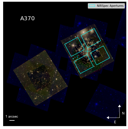
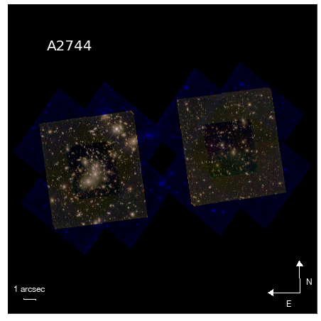
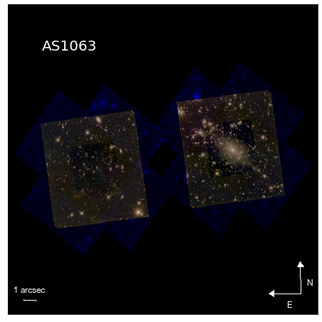
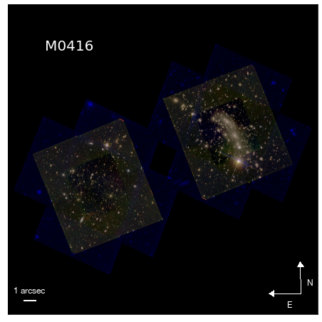
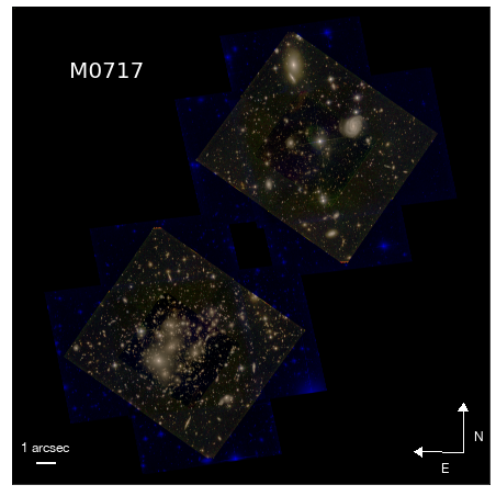
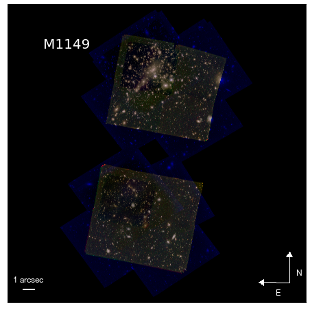
Figure 1: BUFFALO cluster footprints analyzed in this work. The HST mosaics were calibrated, aligned and created following the approaches described in Koekemoer et al. (2011), and the BUFFALO dataset is described in Steinhardt et al. (2020). The RGB color pictures were created using trilogy (Coe et al., 2012), using F160W as the red channel, F105W as the green channel, and F814W as the blue channel. Note that due to the larger area coverage of F814W (ACS) compared to other bands (WFC3), certain areas of the footprint appear as blue. In the top left panel, we include the JWST NIRSpec apertures for reference.

The Hubble Frontier Fields (HFF) (Lotz et al., 2017a) is a multi-waveband program obtaining deep imaging observations of six massive clusters in a narrow redshift range $z\sim 0.308$ - $0.545$. Combining the sensitivity, resolution power and multi-wavelength capability of the Hubble Space Telescope (HST), with the gravitational lensing effect introduced by the massive galaxy clusters selected for this study, one can reach unprecedented depths. Two HST instruments, the Advanced Camera for Surveys (ACS) and Wide-Field Camera 3 (WFC3), were used in parallel to simultaneously observe each cluster and parallel field. The parallel fields separated by $\sim$ 6 arcmin from the cluster core, corresponding to $>1.8$ projected co-moving Mpc for a $z>0.3$ cluster. The six parallel fields are comparable in depth to the Hubble Ultra Deep Field (HUDF, Beckwith et al., 2006), corresponding to m(AB) $\sim$ 29 mag. The area coverage and depth of the parallel fields provide significant improvement in the volume covered and statistics of faint galaxies.

The aims of the HFF observations were: (1) leverage gravitational lensing due to massive clusters (see Kneib & Natarajan, 2011, for a review) to magnify fluxes and hence detect very faint background galaxies at $z$ $\sim 5$ - $10$ (Schneider, 1984; Blandford & Narayan, 1986, and references therein). Strong lensing allows us to probe $\sim$ 2 magnitudes fainter than in blank fields. At the time of HFF observations, blank fields studies reached $\sim$-17 rest-frame UV magnitudes (Finkelstein et al., 2015; Bouwens et al., 2015); (2) study the stellar population of these faint galaxies at high redshifts and constrain the mass function of galaxies at early epochs. Stellar masses reach down to $10^{8}M_{\odot}$ in blank fields (Song et al., 2016; Stefanon et al., 2021; Weaver et al., 2022; Kauffmann et al., 2022) and down to $10^{6}M_{\odot}$ in HFF lensed fields (Bhatawdekar et al., 2019; Kikuchihara et al., 2020; Furtak et al., 2021); (3) study of the morphology and other observable properties of lensed galaxies at $z>8$.

The Beyond Ultra-deep Frontier Fields and Legacy Observations (BUFFALO) is an HST treasury program with 101 prime orbits (and 101 parallel orbits) (GO-15117; PIs: Steinhardt and Jauzac), covering the immediate areas around the HFF clusters where deep Spitzer (IRAC channels 1 and 2) and multi-waveband coverage already exist (Steinhardt et al., 2020). BUFFALO extends the spatial coverage of each of the six HFF clusters by three to four times. Observing these fields in five filters (ACS: F606W, F814W and WFC3: F105W, F125W and F160W), BUFFALO aims at a factor of 2 improvement in the statistics of high redshift galaxies (Furtak et al., 2021, Pagul et al. in prep.), improves the cosmic variance and allows a more accurate modeling of the dark matter distribution in the foreground clusters. The HST and Spitzer data for BUFFALO, combined with ground-based observations (Brammer et al., 2016, KIFF) was specifically designed to expand the HFF to sufficiently large area to encompass a full James Webb Space Telescope NIRSpec field of view, without the need for JWST/NIRCam pre-imaging. The program significantly improves the statistics of galaxies in the outskirts of clusters and field samples.

In this paper, we present photometric and redshift catalogs for the BUFFALO galaxies. The catalogs presented in this work aim to extend and complement previous efforts in the HFF (Merlin et al., 2016a; Castellano et al., 2016; Di Criscienzo et al., 2017; Bradač et al., 2019; Shipley et al., 2018; Nedkova et al., 2021; Pagul et al., 2021). In section 2, we present the data used in this study. In section 3, we briefly outline the data reduction process, referring the reader to Pagul et al. (2021) for a more detailed description. In section 4, we describe our photometric validation procedure. Section 5, details the data products and results. Section 6 describes the photometric redshifts extracted. Finally, our conclusions are presented in section 7.

Throughout this paper we assume standard cosmology with $\Omega_{M}=0.23$, $\Omega_{\Lambda}=0.76$ and $H_{0}=73$ Km/sec/Mpc. Magnitudes are in the AB system.

2 The data

We provide a brief summary of the dataset in the following subsections. For more details about the design, aims and observations of BUFFALO we refer the reader to the BUFFALO overview paper (Steinhardt et al., 2020). All our data products are available at MAST as a High Level Science Product via 10.17909/t9-w6tj-wp63 (catalog 10.17909/t9-w6tj-wp63)

2.1 HST observations

The BUFFALO images provide the deepest exposures of galaxy clusters by HST, only second to the HUDF with respect to depth. With 101 additional prime (and 101 parallel) orbits, they build on the existing HFF cluster and parallel field surveys. BUFFALO slightly increases the depth at the center of the HFF clusters while increasing their areal coverage three- to four fold. As a result, it expands the radial coverage of cluster outskirts, providing observations of the global mass distribution of clusters to almost the virial radius, i.e. $\sim 3/4\times R_{vir}$. The coverage was chosen to increase the high-z sample size, in particular for rare bright high-mass galaxies at $z\sim 8-9$. Furthermore, BUFFALO’s footprint is chosen to be compatible with JWST’s NIRSpec field of view, allowing multiwavelength programs with JWST (Figure 1), which is especially timely for planning robust observations with JWST.

In the HFF, the gravitational potential of the clusters’ halo, besides binding together the galaxies in the system, produces a lensing magnification that could detect background objects to apparent magnitudes of 30–33 mag, i.e. 10–100 times fainter than previous surveys. With BUFFALO, we get magnifications of $\sim 4$ on average. Details of the BUFFALO survey design are provided in Steinhardt et al. (2020). In Table 1, we report the main characteristics of the six clusters, with a summary of the ancillary observations in Table 2. We use the official BUFFALO mosaics, with a pixel scale of 0.06"/pix, which have been produced following the procedures outlined in Koekemoer et al. (2011); the full BUFFALO dataset is described further in Steinhardt et al. (2020).

We complement this data with the available public F275W and F336W HFF data from the HFF-Deepspace campaign (Shipley et al., 2018), which uses observations from Alavi et al. (2016).

2.2 Ancillary data

The large wealth of complementary legacy datasets and programs for the HFF clusters has contributed to its success. The Spitzer Space Telescope dedicated more than 1,000 hours of Director’s Discretionary time to obtain Infrared Array Camera (IRAC) 3.6 $\mu$m (channel 1) and 4.6 $\mu$m (channel 2) imaging down to the depths of 26.5 and 26.0 mag., in cluster and parallel fields respectively (program IDs: Abell 2744: 83, 90275; MACS J0416.1-2403: 80168, 90258; MACS J0717.4+3745: 40652, 60034, 90009, 90259; MACS J1149.4+2223: 60034, 90009, 90260; Abell S1063 (RXC J2248.7-4431): 83, 10170, 60034; Abell 370: 137, 10171, 60034). These observations are especially important for redshift determination given that they help break the degeneracies between low-redshift interlopers and high-redshift galaxies, and are beneficial in constraining galaxy properties since they provide a good proxy for galaxy stellar mass.

The HFF clusters in the southern sky are also covered in the Ks band using the High Acuity Wide Field K-band Imager (HAWK-I) (KIFF Brammer et al., 2016; Pirard et al., 2004; Kissler-Patig et al., 2008) at the Very Large Telescope (VLT), reaching a depth of 26.0 mag (5$\sigma$, point-like sources) for Abell 2744, MACS-0416, Abell S1063, and Abell 370 clusters. In the northern sky, this campaign used the Multi-Object Spectrometer for Infrared Exploration (MOSFIRE) (McLean et al., 2010, 2012) at Keck to observe MACS-0717 and MACS-1149 to a K-band 5$\sigma$ depth of 25.5 and 25.1 mag respectively. This data covers all of the cluster and parallel field centers, but not the entirety of the outer area observed by BUFFALO. Table 2 summarizes the available ancillary data.

Table 1: Frontier Field cluster and parallel field positions, along with clusters’ mean redshift ($z_{\mathrm{clu}}$), virial mass ($M_{\mathrm{vir}}$), and X-ray luminosity ($L_{X}$) (Lotz et al., 2017a)

Field	Cluster Center (J2000)	Parallel Center (J2000)	$z_{\mathrm{clu}}$	$M_{vir}$	$L_{X}$
	R.A., Decl.	R.A., Decl.
Abell 370	02:39:52.9, -01:34:36.5	02:40:13.4, -01:37:32.8	0.375	$\sim 1\times 10^{15}$	$1.1\times 10^{45}$
Abell 2744	00:14:21.2, -30:23:50.1	00:13:53.6, -30:22:54.3	0.308	$1.8\times 10^{15}$	$3.1\times 10^{45}$
Abell S1063	22:48:44.4, -44:31:48.5	22:49:17.7, -44:32:43.8	0.348	$1.4\times 10^{15}$	$1.8\times 10^{45}$
MACS J0416.1-2403	04:16:08.9, -24:04:28.7	04:16:33.1, -24:06:48.7	0.396	$1.2\times 10^{15}$	$1.0\times 10^{45}$
MACS J0717.5+3745	07:17:34.0 +37:44:49.0	07:17:17.0 +37:49:47.3	0.545	$\sim 2-3\times 10^{15}$	$3.3\times 10^{45}$
MACS J1149.5+2223	11:49:36.3, +22:23:58.1	11:49:40.5, +22:18:02.3	0.543	$2.5\times 10^{15}$	$1.8\times 10^{45}$

Table 2: Existing multi-wavelength HFF coverage from follow-up programs, as used in the present work. The 5-$\sigma$ point-source depth was estimated by integrating the noise in a 2D Gaussian PSF aperture with the FWHM value set to the ones given in Table 3. The HFF (Lotz et al., 2017a) program is led by PIs T. Soifer and P. Capak; KIFF PI is G. Brammer (Brammer et al., 2016).

Field	Observatory/Camera	Central Wavelength	Depth
Abell 370	VLT/HAWK-I	2.2$\mu m$	$\sim$ 26.18
	Spitzer IRAC 1,2	3.6$\mu m$, 4.5$\mu m$	$\sim$ 25.19, 25.09
MACS J0717.5+3745	Keck/MOSFIRE	2.2$\mu m$	$\sim$ 25.31
	Spitzer IRAC 1,2	3.5$\mu m$, 4.5 $\mu m$	$\sim$ 25.04, 25.17
MACS J0416.1-2403	VLT/HAWK-I	2.2$\mu m$	$\sim$ 26.25
	Spitzer IRAC 1,2	3.5$\mu m$, 4.5 $\mu m$	$\sim$ 25.31, 25.44
Abell S1063	VLT/HAWK-I	2.2$\mu m$	$\sim$ 26.31
	Spitzer IRAC 1,2	3.6$\mu m$, 4.5$\mu m$	$\sim$ 25.04, 25.04
Abell 2744	VLT/HAWK-I	2.2$\mu m$	$\sim$ 26.28
	Spitzer IRAC 1,2	3.6$\mu m$, 4.5$\mu m$	$\sim$ 25.32, 25.08
MACS J1149.5+2223	Keck/MOSFIRE	2.2$\mu m$	$\sim$ 25.41
	Spitzer IRAC 1,2	3.5$\mu m$, 4.5 $\mu m$	$\sim$ 25.24, 25.01

Table 3: The Point Spread Function radius and effective wavelengths for different photometric bands used for the BUFFALO fields.

Band	$FWHM$	$\lambda_{\mathrm{pivot}}$ (Å)
F275W	0$\farcs$11	2710
F336W	0$\farcs$12	3354
F435W	0$\farcs$13	4329
F606W	0$\farcs$11	5922
F814W	0$\farcs$10	8045
F105W	0$\farcs$20	10551
F125W	0$\farcs$20	12486
F140W	0$\farcs$20	13923
F160W	0$\farcs$20	15369
Ks	0$\farcs$36	21524
I1	1$\farcs$29	35634
I2	1$\farcs$42	45110

Note. — Values were calculated for the cluster Abell 370.

3 Data processing

The workflow followed for the data processing in this work is the same as the one in Pagul et al. (2021) (P21 hereafter). The main steps taken to obtain the data products presented here are summarized as follows:

1. Error map correction: we compare the standard deviation of the values of the background pixels in the science image, with the reported root mean-square (rms) values as given by the error maps, and correct the latter so that the mean ratio in the background pixels are equal to $1$.

2. PSF extraction: we select unsaturated, unblended stars and perform median stacking to obtain an estimate of the PSF.

3. Intracluster light (ICL) + bright galaxy modeling: Perform multi-object fits to Sérsic profiles, plus a local background using a combination of GALFIT (Peng et al., 2010) and GALAPAGOS-M (Häußler et al., 2013).

4. Bright galaxy photometry: we run Source Extractor (Bertin & Arnouts, 1996) on HST bands PSF-matched to the reddest, F160W, band, and obtain photometric measurements.

5. Background galaxy photometry: we subtract the bright galaxies and ICL, and run Source Extractor on the “cleaned” field for the PSF-matched HST images.

6. Spitzer and K-band photometry: we use T-PHOT (Merlin et al., 2016b) to obtain self-consistent photometry measurements on the Spitzer and K-band images, using the HST images and segmentation maps as priors.

7. Synthetic source injection: we inject synthetic sources and repeat the process to validate and correct the photometric measurements.

8. Estimate photometric redshifts: the last step consists on using LePhare (Arnouts et al., 1999; Ilbert et al., 2006) to obtain photometric redshift estimates of detected galaxies in these catalogs.

In the following subsections some of these steps are described in more detail. For a detailed description of all the steps, we refer the reader to P21.

3.1 Point Spread Function

A well-defined point spread function (PSF) as a function of wavelength is crucial to perform consistent photometry within a ‘panchromatic’ baseline to correctly model galaxies and obtain galaxy fluxes in PSF-matched images. In order to perform multi-waveband photometry with accurate signal-to-noise and resolution for each aperture, we convolve images with a kernel generated by taking (in Fourier space) the ratio between their original and target PSFs, to match that of the reddest F160W PSF. In order to generate the PSFs for the HST and K-band images, we stack isolated and unsaturated stars in each individual image, taking the median of the stack. Up to this point, the procedure is identical to that followed in P21. We improve upon our previous work by creating PSFs for the representative inner (deeper) and outer (shallower) regions in both the cluster- and parallel-fields. Figure 2 shows examples of the stacked PSFs derived in different regions, and Table 3 gives the representative FWHM as a function of wavelength. We note that the full-width-half-max (FWHM) in both regions are compatible.

Due to large spatial variations of the PSF in the mid-IR Spitzer channels , we do not use the same approach to create our Spitzer PSF model. Furthermore, the individual pixel response functions (PRFs) are asymmetric and are thus dependent on the orientation of the camera. Moreover, the pixels on IRAC Ch 1 and 2 tend to under sample the PRF. Thus, instead of stacking stars and generating a single PSF per field, we use a synthetic pixel response function (PRF) that combines the information on the PSF, the detector sampling, and the intrapixel sensitivity variation in response to a point-like source, as done in P21. A PRF model for a given position on the IRAC mosaic is generated by the code PRFMap (A. Faisst, private communication) by combining the single-epoch frames that contribute to that mosaic. To do so, PRFMap stacks individual PRF models with the same orientation of the frames, resulting in a realistic, spatially-dependent PSF model.

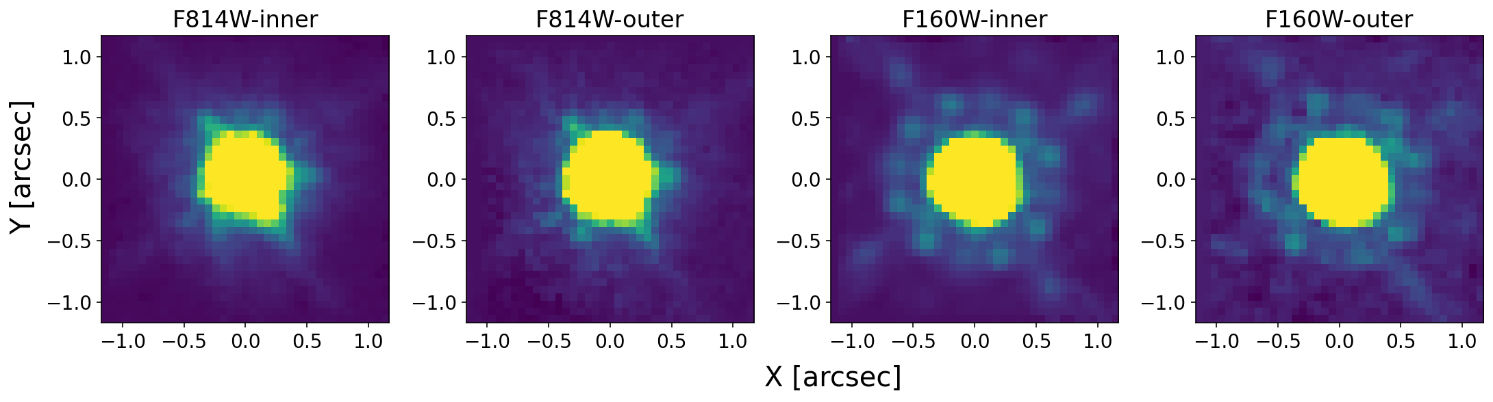
Figure 2: Representative examples of the point spread function (PSF) for the instruments used in this study, corresponding to a 0.06"/pixel scale normalized with the ZScale algorithm. From left to right, panels show ACS-F814W (inner region), ACS-F814W (outer region), WFC3-F160W (inner region), WFC3-F160W (outer region). See Section 3.1 for more details

3.2 Modeling the intra-cluster light

The deep potential well and high density of galaxy clusters make them rich laboratories to study galaxy dynamics and interactions. Due to these complex processes, stars and gas stripped from their constituent galaxies build up in the cluster core as intracluster light (ICL) (see Montes, 2022, for a review). This can bias the flux measurements of galaxies, close in angular space, to the cluster center. Following Morishita et al. (2017) and P21, in order to model the ICL in the BUFFALO clusters, we first generate $18\times 18$ arcsecond ($300\times 300$ pixel) stamps centered on each galaxy with a magnitude brighter than 26 in each image/band. Using GALFIT (Peng et al., 2010), we fit all galaxies in each stamp with a single Sérsic profile, masking those that are fainter than magnitude 26. In case a given pixel with coordinates $(x,y)$ is only included in one cutout, the ICL emission ($F_{\mathrm{ICL}}$) is defined as the local background measurement as reported by GALFIT (namely, the sky value parameter). If there are overlapping cutouts in $(x,y)$, we use the inverse $\chi^{2}$-weighted mean of their background measurements:

$$F_{\mathrm{ICL}}(x,y)=\frac{\Sigma_{i}s_{i}(x,y)/\chi^{2}_{i}(x,y)}{\Sigma_{i}1/\chi^{2}_{i}(x,y)}\;,$$ (1)

where $s_{i}$ and $\chi_{i}^{2}$ are the sky fit (fit value to the local background of the postage stamp) and goodness-of-fit values from GALFIT for the $i$-th cutout, respectively.

As described in P21, the resulting ICL map has unphysical sharp features, which are smoothed out using a Gaussian kernel with $\sigma=4.32"$.

Similarly, for the $K_{s}$ and $Spitzer$ bands, we use T-PHOT to obtain the local background for each measured source, which is then merged into a single mosaic, and smoothed with a representative kernel.

As a caveat, though these maps primarily contain ICL emission, they also contain inhomogeneities in the background. This ensures a robust ‘background$+$ICL subtraction" in the individual images. Cleaning of these maps via color selection of the individual stamps will then be performed.

3.3 Modeling the brightest galaxies

The procedure to model bright galaxies (magnitude brighter than 19) is also unchanged from P21. We rely on GALAPAGOS-M (Häußler et al., 2013) to fit Sérsic profiles simultaneously to galaxies in all bands, with the fitting parameters varying as a function of wavelength. We construct galaxy models for the relevant galaxies and also cross-check the fits with those in Nedkova et al. (2021). The results of the ICL and bright galaxy modeling and subtraction are illustrated in Figure 3.

Finally, we apply a median filter to the ICL+bright galaxy subtracted images. We use a filter with a box size of 1^∘ per side, applied only to pixels within 1$\sigma$ of the background level to reduce the effects of over-subtraction in the residual. Figure 3 shows the modeling and filtering process. The lower right panel shows the effect of median filtering. Note that this process does not significantly affect the outskirts of the cluster.

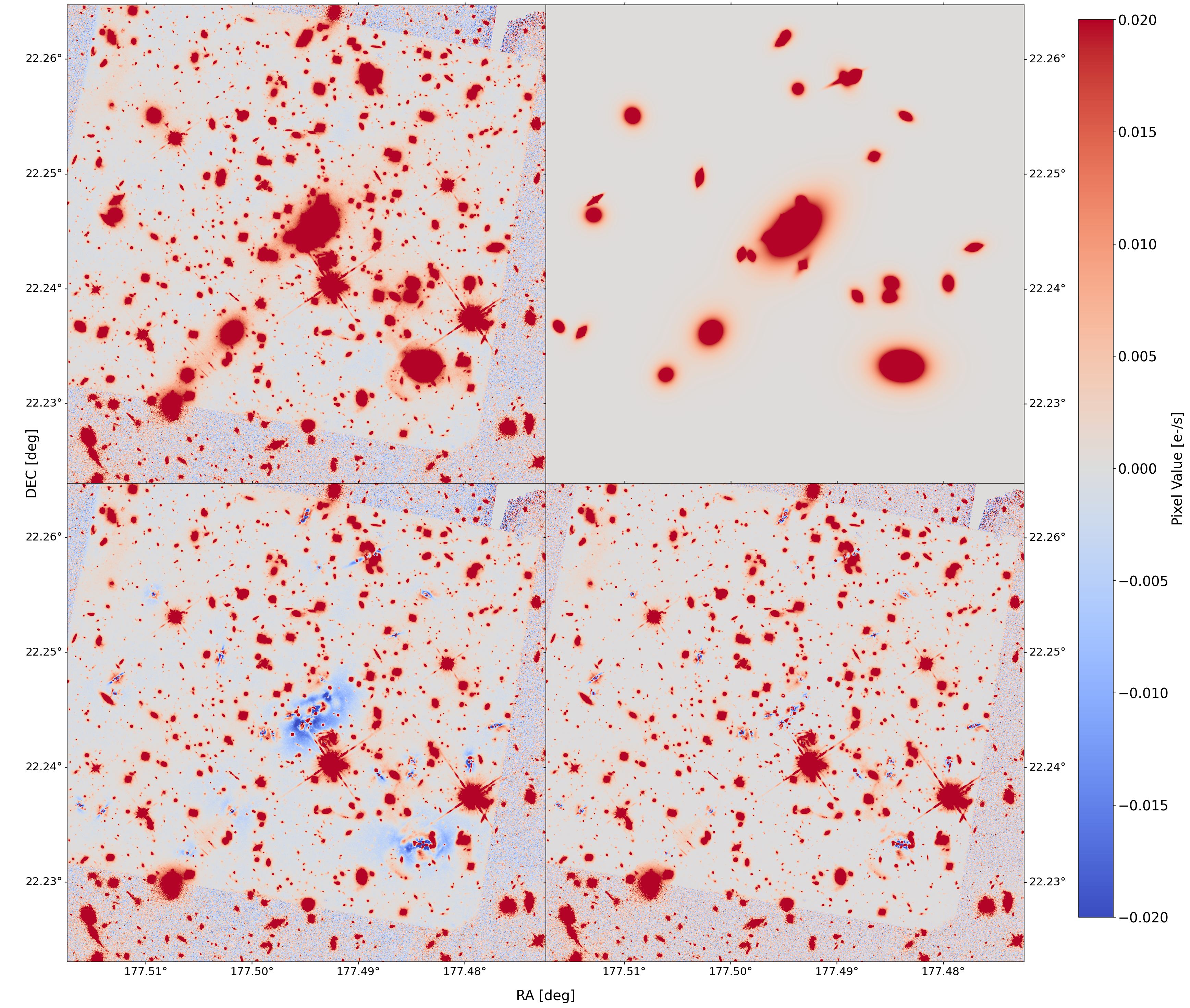
Figure 3: Steps in bright cluster + ICL modelling (in this case for cluster MACS 1149) for the F160W band. Upper panels show the original image (left) and the galaxy/ICL models (right). Lower panels show the residual image before and after median filtering (left- and right-hand panel respectively). The colorbar denotes the pixel intensity in counts/s. See Sections from 3.2 to 3.3 for more details.

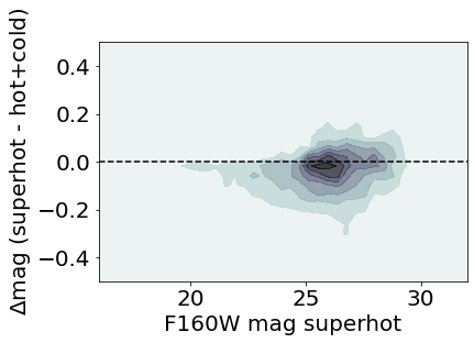
Figure 4: Magnitude comparison between “hot+cold" mode as described in P21, and the “super hot" mode used in this work. Note, the magnitude difference is primarily within 0.05 mags.

3.4 Source Extraction

To detect galaxies and perform photometry, we use Source Extractor, focusing only on the "super hot" mode, rather than creating a dual run with hot and cold modes (see P21 for definition of "hot" and "cold" modes). This is one of the main differences with the procedure presented in P21 where a second “cold" mode Source Extractor run is performed. We find that this second run does not have a significant impact on the detection nor photometric performance ($<0.05$ mag), especially after bright galaxy and ICL subtraction. This is a consequence of the cold mode focusing on extracting information about the brightest objects, which have already been removed by the bright galaxy subtraction. This is illustrated in Figure 4, where we compare a dual run with our new “super hot" run, finding similar magnitudes for the BUFFALO cluster Abell 370. The final Source Extractor configuration file is presented in Appendix B.

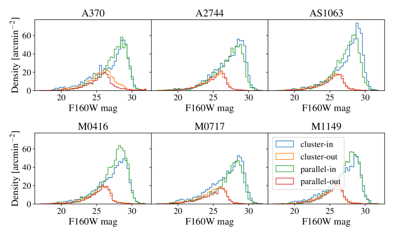
Figure 5: Magnitude distributions for sources in the BUFFALO catalogs across all clusters. We subdivide each of the catalogs, one per cluster and per parallel/infall field, into inner (in) and outer (out) regions, which correspond to different depth regimes.

We also show the magnitude distribution of sources in the F160W band for all clusters in Figure 5. The large number density (defined as the number of sources per square arcmin) and depth of these catalogs are indicated. We subdivided the catalogs into sources detected in the inner field regions (the overlap with HFF), which reaches to significant depth, and the outer regions (the extension), where the depth is noticeably lower. The differences between the distributions of the cluster and the parallel regions is apparent. The cluster regions typically contain an over-abundance of brighter galaxies, whereas the parallel fields contain less of these bright objects but reach slightly deeper levels.

3.5 Photometry in Ancillary images

Because the Ks and Spitzer images have lower angular resolution than the HST images, they are more affected by blending. In order to effectively deblend sources and maximize the information extracted in each image, we use T-PHOT as in P21 to perform forced photometry in the Ks- and IRAC images on sources detected in the IR-Weighted HST image. T-PHOT (Merlin et al., 2015, 2016b) is a software that uses priors from high resolution data in order to deblend and extract fluxes of the same objects in a lower resolution image. We first use T-PHOT’s built-in background routine to generate a local background for each source and remove the excess ICL light as well as inhomogenieties in the backgrounds. Then, as “real” galaxy priors, we use the IR-Weighted segmentation map and flux measurements from the F160W-band image. Additionally, we use the galaxy models that have been created in the bright galaxy$+$ICL removal step as the “model” priors. Given the spatial variation of the PRF in the IRAC bands, we take advantage of T-PHOT’s “multikernel” option, and use a separate PRF to model sources at each position. We emphaize that the flux (FitQty) that is provided by T-PHOT corresponds to the total flux emitted by a given source.

4 Photometric validation

In order to characterize the performance of our detection and measurement procedures, we proceed as in P21 injecting synthetic galaxies in the original BUFFALO images using GalSim (Rowe et al., 2015) to render noiseless realistic galaxies via the RealGalaxy class following the morphology measurements in COSMOS by Leauthaud et al. (2007). This catalog only contains information for fluxes in the F814W band. Thus, we match these sources to the COSMOS catalog (Laigle et al., 2016a) in order to obtain the fluxes in the rest of our bands of interest. We choose to keep the morphology and centroids fixed across bands in order to simplify data handling and bookkeeping. In this case, we generate 10 realizations of a set of 160 sources using the F160W image footprint as reference. Note that, since not all bands cover the same footprint, some sources will not be recovered after processing. We then insert these sources in the original images, run our pipeline on the resulting combined image (which is the sum of the original and the noiseless synthetic sources) and compare their measured fluxes and positions to their inputs.

This provides valuable information about completeness and absolute zeropoint calibration. The two catalogs are matched using a nearest neighbor matching routine, match_coordinates_sky, included in the astropy package Astropy Collaboration et al. (2013, 2018). The results of this comparison are shown in Figure 6. We see that for all of the HST bands (F435W, F606W, F814W, F105W, F125W, F140W, F160W) the recovered magnitude is within 20 mmags of the input, and that the reconstruction of the fluxes is relatively stable across the considered range of magnitudes. We note that at the bright end, there is a small fraction of the flux missing, probably due to the extended tails of the sources not being captured by the aperture. This photometric bias becomes smaller with increasing magnitude up to the point where we start to lose sensitivity. We use these offsets to robustly correct the fluxes in each band. For Ks the performance is also excellent and we find a median value of $\Delta\rm{mag}=-0.05\rm{mag}$. For the Spitzer IRAC channels, we find a small photometric offset $\Delta\rm{mag}=-0.12$ and $\Delta\rm{mag}=-0.13$ for I1 and I2, respectively.

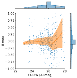
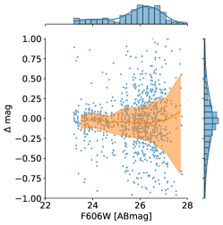
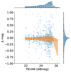
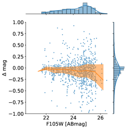
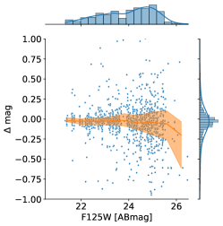
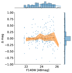
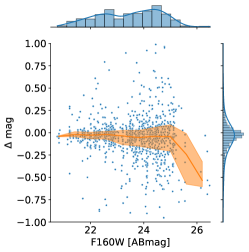
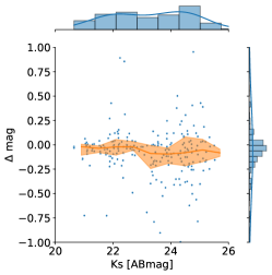
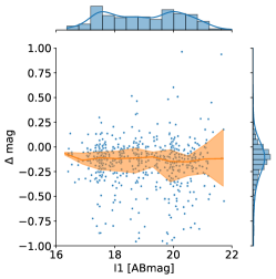
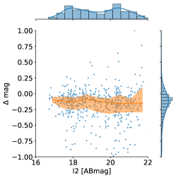
Figure 6: Photometric validation of the BUFFALO catalogs. Scatter plot of $\Delta\rm{mag}=\rm{mag}_{in}-\rm{mag}_{out}$ as a function of the input magnitude for the different bands considered in this work. The solid line shows the rolling mean magnitude offset and the shaded area corresponds to the inter-quartile range. Additionally, each panel includes the input magnitude histogram (top horizontal histogram) as well as the $\Delta\rm{mag}$ histogram (right vertical histogram).

We compare the mean uncertainty reported by the measurement pipeline to the standard deviation of $\Delta\rm{mag}$ as a function of magnitude. Again, for the HST bands the performance is excellent, and we find that the reported errors are in good agreement with the scatter measured using our synthetic sources. This is not the case for Ks nor IRAC, where we find that a correction is needed. In particular, we use a power-law correction:

$$\Delta F_{new}=\Delta F_{old}AF^{B},$$ (2)

where $\Delta F_{new}$ is the corrected uncertainty estimate, $\Delta F_{old}$ is the reported uncertainty by the measurement software, $F$ is the reported flux, and $A$, $B$ are free parameters. We fit $A$, $B$ and tabulate the results in Table 4.

Band	$A$ [counts/s]-1	$B$
Ks	2.05	0.26
I1	164.67	0.44
I2	123.14	0.43

Table 4: Best-fit coefficients used to perform the uncertainty correction as a function of flux.

5 Data products and results

In this section, we discuss the data products from this work and present some validation results. We produce several new data products from BUFFALO, including catalogs, models for the point spread function, and models for the ICL and bright galaxies. The final catalogs include properties of >100,000 sources in the 6 BUFFALO cluster and parallel fields, and extend the Frontier Fields footprint, covering a total of $\sim 240$ square-arcminutes. These include positions, multi-waveband photometry, and photometric redshift estimates for the sources detected as provided by LePhare (Arnouts et al., 1999; Ilbert et al., 2006). Additional details about the information provided by these catalogs can be found in Appendix A.

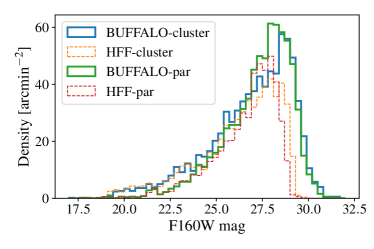
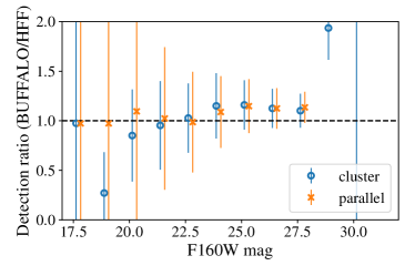
Figure 7: Top panel: Comparison of magnitude distribution in the F160W band between BUFFALO sources (solid lines) and HFF (broken lines) for both the cluster and parallel (par) fields in the deepest part of the images for MACS J1149. Bottom panel: Ratio between the histograms in the top panel for the cluster field (blue open circles) and parallel field (orange crosses). Other fields show similar behavior

Point spread function (PSF) estimates are provided as as FITS images. Section 3.1 describes the modeling of the PSFs. We summarize some of their properties in Table 3. Unsurprisingly, these results are very similar to those found by P21, as the BUFFALO fields are mostly extensions of the HFF.

The procedure to obtain models for the ICL and bright galaxies is described in Section 3.3. These models are also available as FITS images.

5.1 Photometric redshifts

In this section we present our redshift estimates based on the photometric measurements presented in previous sections. We run LePhare  (Arnouts et al., 1999; Ilbert et al., 2006), a template-based code that derives a redshift likelihood function for each source. As in P21, the fluxes used as inputs to LePhare are rescaled by a factor:

$$f_{\mathrm{tot}}=\frac{\sum_{i}w_{i}(\mathrm{FLUX\_AUTO}/\mathrm{FLUX\_ISO})_{i}}{\sum_{i}w_{i}},$$ (3)

i.e. the weighted mean of the AUTO-to-ISO flux ratio summed over the observed HST bands, where the weights, $w_{i}$, are the sum in quadrature of the Source Extractor errors: $w_{i}=\sqrt{\sigma_{i,\mathrm{AUTO}}^{2}+\sigma_{i,\mathrm{ISO}}^{2}}$. This is done in order to improve the accuracy of the colors. For the TPHOT-based photometry (Ks, and IRAC bands), as we do not have an equivalent to FLUX_ISO, we include our baseline fluxes. The template library, and dust attenuation follows Laigle et al. (2016b), using Prevot et al. (1984) or Calzetti et al. (2000) extinction laws depending on the galaxy type. For details about the templates and the extinction prescriptions we refer the reader to Laigle et al. (2016b) and P21. In our catalog the redshift estimates, ZPDF, correspond to the position of the maximum-likelihood for each object.

The redshift calibration procedure is similar to that presented in P21, which is based on spectroscopic data described in Owers et al. (2011); Ebeling et al. (2014); Richard et al. (2014); Balestra et al. (2016); Treu et al. (2015); Schmidt et al. (2014); Jauzac et al. (2015); Grillo et al. (2016); Treu et al. (2016); Lagattuta et al. (2017); Mahler et al. (2018); Lagattuta et al. (2019). We obtain the best-fit template for each source and try to find a systematic offset in each band by comparing the predicted and observed flux for all sources that have a measured spectroscopic redshift with a spectroscopic quality flag $>3$. These magnitude offsets, when applied to the photometric baseline, compensate for a possible bias in the template library and/or for calibration issues in data reduction. We find these corrections to be below 9% for all the HST bands. For the $K_{\mathrm{s}}$ band, we find a correction of $0.883$ while in the IRAC channels 1 and 2, the correction is a factor $1.117$ and $1.182$, respectively. These corrections are shown in Table 5.

Figure 10 also shows the photometric redshift distribution for objects in each cluster, estimated from the SED fits with a reduced $\chi^{2}<$ 10.

Table 5: Multiplicative factors applied to each band in the photo-z calibration step.

Band	Multiplicative Factor
F275W	1.055
F336W	1.011
F435W	1.085
F475W	1.060
F606W	1.004
F625W	1.006
F814W	0.992
F105W	1.004
F110W	1.015
F125W	1.011
F140W	1.008
F160W	0.995
Ks	0.883
IRAC1	1.117
IRAC2	1.182

6 Comparison with the Hubble Frontier Fields

By design, there is significant overlap between the HFF and the BUFFALO fields. This makes the HFF catalogs an exceptional reference to verify and validate the data presented in this work and to check for potential improvements, given the increased number of exposures. Here, we compare our BUFFALO data products with those presented in P21.

Figure 7 compares the magnitude distribution of sources in the F160W band between the catalog presented here and the catalogs in P21 in the overlapping region of the MACS J1149 cluster. Here we show that our new BUFFALO catalogs reach fainter sources than those from the HFF. We also show the fraction of detected objects as a function of magnitude, finding that both catalogs have a similar completeness to magnitude $\sim 27.5$ in the F160W band. This is in agreement with P21, where the completeness dropped below 100% at $\sim 27.5$. Other bands and clusters show a similar behavior. We note that these completeness estimates do not take into account the effects of strong lensing.

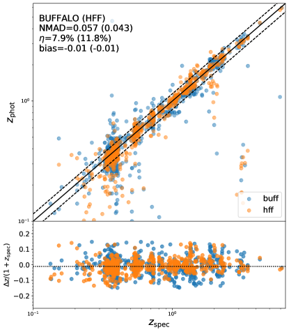
Figure 8: Assessing the quality of photometric redshifts estimated through SED fitting. Top panel: Photometric vs. spectroscopic redshift comparison. Blue and orange points are 709 matched BUFFALO and HFF sources, respectively, whose with BUFFALO F160W band magnitude are between 16 and 26, are detected in at least 5 BUFFALO bands, with a redshift quality flag > 3. The solid line shows the 1:1 relationship, and the dashed lines encloses the $z_{phot}=z_{spec}\pm 0.15(1+z_{spec})$ threshold used to identify outliers (i.e., catastrophic errors). NMAD scatter ($\sigma$) and outlier fraction ($\eta$) are reported on the top-left corner. Bottom panel: $\Delta z\equiv z_{phot}-z_{spec}$ scatter.

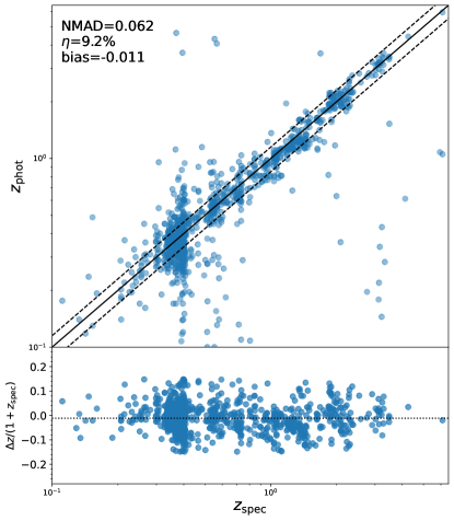
Figure 9: Assessing the quality of photometric redshifts estimated through SED fitting. Top panel: Photometric vs. spectroscopic redshift comparison. Blue points are 999 spectroscopic redshifts selected for 16 < F 160W < 26, detected in at least 5 bands, with a redshift quality flag > 3. The solid line shows the 1:1 relationship and the dashed lines encloses the zphot = zspec$\pm$0.15(1$+$zspec) threshold used to identify outliers (i.e., catastrophic errors). The median of $\Delta z/(1+z_{spec})$ (bias) and outlier fraction ($\eta$) are reported on the top-left corner. Bottom panel: $\Delta$z $\equiv$ zphot $-$ zspec scatter.

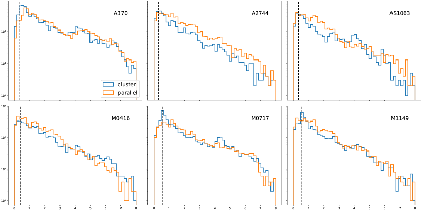
Figure 10: Redshift histograms for each cluster field. Dotted line corresponds to the redshift of the cluster. Sources were chosen with mag$AB_{F160W}<28.5$ and $\chi^{2}/\rm{ndof}<5$.

7 Summary

The wealth of deep (HST) observations and ancillary data in the HFF (Lotz et al., 2017b), open a window to the high-redshift universe, and provides a complementary sample to the JWST. The BUFFALO survey (Steinhardt et al., 2020, PIs: Mathilde Jauzac, Charles Steinhardt) used these data and extended the observations in the 6 HFFs, to allow for follow-up spectroscopy. This work presents a new set of data products based on the BUFFALO observations. The data products include models for the point spread function (PSF), intra-cluster light (ICL), the bright galaxies, and catalogs of astronomical sources. The catalogs contain detailed information (including positions and photometry) of over 100,000 sources distributed across 6 separate cluster and parallel fields covering a total area of 240 arcmin².

The data products are obtained using a similar procedure to that outlined in Pagul et al. (2021). First, a model of the bright galaxies, and the ICL are created. These models are then subtracted from the original image, in order to increase our sensitivity allowing us to observe fainter sources, which are detected and measured using Source Extractor in the HST bands. We then use the IR-weighted segmentation map as priors in the T-PHOT package to obtain forced-photometry in ancillary data from Keck $K$s band, and Spitzer IRAC channels 1 and 2. The photometric measurements are validated using synthetic source injection. Finally, LePhare is run to obtain redshift estimates based on our photometric measurements. The main change with respect to the procedure in P21 is the usage of a “super hot” mode Source Extractor run, that simplifies bookkeping, while not biasing the photometric estimates. As a sanity check, we plot the redshift histograms and note that the peaks of these histograms correspond to the redshift of each respective cluster.

This catalog represents one of the deepest views at galaxy clusters to date and a sample that lends itself well for JWST follow-up. All of the data products presented in this work will be made publicly available to the astronomical community through the usual astronomical archive databases (MAST and Vizier).

Appendix A Catalog details

The catalogs presented in this work contain the following information:

• ID: Source number

• FLUX_FXXXW: Total scaled flux in cgs units of $\mathrm{erg/cm}^{2}\mathrm{/s/Hz}$

• FLUXERR_FXXXW: Corrected flux error in cgs units of $\mathrm{erg/cm}^{2}\mathrm{/s/Hz}$

• ZSPEC: reported spectroscopic redshift

• ZSPEC_Q: reported quality flag of spectroscopic redshift

• ZSPEC_REF: dataset from which spectroscopic redshift was obtained

• ALPHA_J2000_STACK: Right Ascension (J2000) in degrees using GAIA DR2 as reference.

• DELTA_J2000_STACK: Declination (J2000) in degrees using GAIA DR2 as reference.

• FIELD: denotes the field object belongs to

• ZCHI2: photometric redshift goodness of fit

• CHI2_RED: reduced chi square

• ZPDF: photometric redshift derived via maximum likelihood

• ZPDF_LOW: lower threshold for photometric redshift

• ZPDF_HIGH: upper threshold for photometric redshift

• MOD_BEST: galaxy model for best $\chi^{2}$

• EXT_LAW: Extinction law

• E_BV: E(B-V)

• ZSECOND: secondary photometric redshift peak in maximum likelihood distribution

• BITMASK: Base 2 number to determine which bands were used. Calculated via bitmask$=\sum_{n=goodbandindex}2^{n}$

• NB_USED: number of bands used

Appendix B Source Extractor Configuration

DETECT_MINAREA 3

DETECT_THRESH 0.5

ANALYSIS_THRESH 0.5

FILTER Y

FILTER_NAME gauss_4.0_7x7.conv

DEBLEND_NTHRESH 64

DEBLEND_MINCONT 0.000005

CLEAN Y

CLEAN_PARAM 0.8

MASK_TYPE CORRECT

PHOT_AUTOPARAMS 2.0, 3.5

PHOT_FLUXFRAC 0.5

SEEING_FWHM 0.17

STARNNW_NAME goods_default.nnw

BACK_SIZE 64

BACK_FILTERSIZE 3

BACKPHOTO_TYPE LOCAL

BACKPHOTO_THICK 24

References

- Alavi et al. (2016) Alavi, A., Siana, B., Richard, J., et al. 2016, ApJ, 832, 56, doi: 10.3847/0004-637X/832/1/56
- Arnouts et al. (1999) Arnouts, S., Cristiani, S., Moscardini, L., et al. 1999, MNRAS, 310, 540, doi: 10.1046/j.1365-8711.1999.02978.x
- Astropy Collaboration et al. (2013) Astropy Collaboration, Robitaille, T. P., Tollerud, E. J., et al. 2013, A&A, 558, A33, doi: 10.1051/0004-6361/201322068
- Astropy Collaboration et al. (2018) Astropy Collaboration, Price-Whelan, A. M., Sipőcz, B. M., et al. 2018, AJ, 156, 123, doi: 10.3847/1538-3881/aabc4f
- Balestra et al. (2016) Balestra, I., Mercurio, A., Sartoris, B., et al. 2016, ApJS, 224, 33, doi: 10.3847/0067-0049/224/2/33
- Beckwith et al. (2006) Beckwith, S. V. W., Stiavelli, M., Koekemoer, A. M., et al. 2006, AJ, 132, 1729, doi: 10.1086/507302
- Bertin & Arnouts (1996) Bertin, E., & Arnouts, S. 1996, A&AS, 117, 393, doi: 10.1051/aas:1996164
- Bhatawdekar et al. (2019) Bhatawdekar, R., Conselice, C. J., Margalef-Bentabol, B., & Duncan, K. 2019, MNRAS, 486, 3805, doi: 10.1093/mnras/stz866
- Blandford & Narayan (1986) Blandford, R., & Narayan, R. 1986, ApJ, 310, 568, doi: 10.1086/164709
- Bouwens et al. (2015) Bouwens, R. J., Illingworth, G. D., Oesch, P. A., et al. 2015, ApJ, 803, 34, doi: 10.1088/0004-637X/803/1/34
- Bradač et al. (2019) Bradač, M., Huang, K.-H., Fontana, A., et al. 2019, MNRAS, 489, 99, doi: 10.1093/mnras/stz2119
- Brammer et al. (2016) Brammer, G. B., Marchesini, D., Labbé, I., et al. 2016, The Astrophysical Journal Supplement Series, 226, 6, doi: 10.3847/0067-0049/226/1/6
- Calzetti et al. (2000) Calzetti, D., Armus, L., Bohlin, R. C., et al. 2000, ApJ, 533, 682
- Castellano et al. (2016) Castellano, M., Amorín, R., Merlin, E., et al. 2016, A&A, 590, A31, doi: 10.1051/0004-6361/201527514
- Coe et al. (2012) Coe, D., Umetsu, K., Zitrin, A., et al. 2012, ApJ, 757, 22, doi: 10.1088/0004-637X/757/1/22
- Di Criscienzo et al. (2017) Di Criscienzo, M., Merlin, E., Castellano, M., et al. 2017, A&A, 607, A30, doi: 10.1051/0004-6361/201731172
- Ebeling et al. (2014) Ebeling, H., Ma, C.-J., & Barrett, E. 2014, ApJS, 211, 21, doi: 10.1088/0067-0049/211/2/21
- Finkelstein et al. (2015) Finkelstein, S. L., Ryan, Russell E., J., Papovich, C., et al. 2015, ApJ, 810, 71, doi: 10.1088/0004-637X/810/1/71
- Furtak et al. (2021) Furtak, L. J., Atek, H., Lehnert, M. D., Chevallard, J., & Charlot, S. 2021, MNRAS, 501, 1568, doi: 10.1093/mnras/staa3760
- Grillo et al. (2016) Grillo, C., Karman, W., Suyu, S. H., et al. 2016, ApJ, 822, 78, doi: 10.3847/0004-637X/822/2/78
- Häußler et al. (2013) Häußler, B., Bamford, S. P., Vika, M., et al. 2013, MNRAS, 430, 330, doi: 10.1093/mnras/sts633
- Ilbert et al. (2006) Ilbert, O., Arnouts, S., McCracken, H. J., et al. 2006, A&A, 457, 841, doi: 10.1051/0004-6361:20065138
- Jauzac et al. (2015) Jauzac, M., Richard, J., Jullo, E., et al. 2015, MNRAS, 452, 1437, doi: 10.1093/mnras/stv1402
- Kauffmann et al. (2022) Kauffmann, O. B., Ilbert, O., Weaver, J. R., et al. 2022, arXiv e-prints, arXiv:2207.11740. https://arxiv.org/abs/2207.11740
- Kikuchihara et al. (2020) Kikuchihara, S., Ouchi, M., Ono, Y., et al. 2020, ApJ, 893, 60, doi: 10.3847/1538-4357/ab7dbe
- Kissler-Patig et al. (2008) Kissler-Patig, M., Pirard, J. F., Casali, M., et al. 2008, A&A, 491, 941, doi: 10.1051/0004-6361:200809910
- Kneib & Natarajan (2011) Kneib, J.-P., & Natarajan, P. 2011, A&A Rev., 19, 47, doi: 10.1007/s00159-011-0047-3
- Koekemoer et al. (2011) Koekemoer, A. M., Faber, S. M., Ferguson, H. C., et al. 2011, ApJS, 197, 36, doi: 10.1088/0067-0049/197/2/36
- Lagattuta et al. (2017) Lagattuta, D. J., Richard, J., Clément, B., et al. 2017, MNRAS, 469, 3946, doi: 10.1093/mnras/stx1079
- Lagattuta et al. (2019) Lagattuta, D. J., Richard, J., Bauer, F. E., et al. 2019, MNRAS, 485, 3738, doi: 10.1093/mnras/stz620
- Laigle et al. (2016a) Laigle, C., McCracken, H. J., Ilbert, O., et al. 2016a, ApJS, 224, 24, doi: 10.3847/0067-0049/224/2/24
- Laigle et al. (2016b) —. 2016b, ApJS, 224, 24, doi: 10.3847/0067-0049/224/2/24
- Leauthaud et al. (2007) Leauthaud, A., Massey, R., Kneib, J.-P., et al. 2007, ApJS, 172, 219, doi: 10.1086/516598
- Lotz et al. (2017a) Lotz, J. M., Koekemoer, A., Coe, D., et al. 2017a, ApJ, 837, 97, doi: 10.3847/1538-4357/837/1/97
- Lotz et al. (2017b) —. 2017b, ApJ, 837, 97, doi: 10.3847/1538-4357/837/1/97
- Mahler et al. (2018) Mahler, G., Richard, J., Clément, B., et al. 2018, MNRAS, 473, 663, doi: 10.1093/mnras/stx1971
- McLean et al. (2010) McLean, I. S., Steidel, C. C., Epps, H., et al. 2010, in Society of Photo-Optical Instrumentation Engineers (SPIE) Conference Series, Vol. 7735, Ground-based and Airborne Instrumentation for Astronomy III, ed. I. S. McLean, S. K. Ramsay, & H. Takami, 77351E
- McLean et al. (2012) McLean, I. S., Steidel, C. C., Epps, H. W., et al. 2012, in Society of Photo-Optical Instrumentation Engineers (SPIE) Conference Series, Vol. 8446, Ground-based and Airborne Instrumentation for Astronomy IV, ed. I. S. McLean, S. K. Ramsay, & H. Takami, 84460J
- Merlin et al. (2015) Merlin, E., Fontana, A., Ferguson, H. C., et al. 2015, A&A, 582, A15, doi: 10.1051/0004-6361/201526471
- Merlin et al. (2016a) Merlin, E., Amorín, R., Castellano, M., et al. 2016a, A&A, 590, A30, doi: 10.1051/0004-6361/201527513
- Merlin et al. (2016b) Merlin, E., Bourne, N., Castellano, M., et al. 2016b, A&A, 595, A97, doi: 10.1051/0004-6361/201628751
- Montes (2022) Montes, M. 2022, Nature Astronomy, 6, 308, doi: 10.1038/s41550-022-01616-z
- Morishita et al. (2017) Morishita, T., Abramson, L. E., Treu, T., et al. 2017, ApJ, 846, 139, doi: 10.3847/1538-4357/aa8403
- Nedkova et al. (2021) Nedkova, K. V., Häußler, B., Marchesini, D., et al. 2021, MNRAS, 506, 928, doi: 10.1093/mnras/stab1744
- Owers et al. (2011) Owers, M. S., Randall, S. W., Nulsen, P. E. J., et al. 2011, ApJ, 728, 27, doi: 10.1088/0004-637X/728/1/27
- Pagul et al. (2021) Pagul, A., Sánchez, F. J., Davidzon, I., & Mobasher, B. 2021, ApJS, 256, 27, doi: 10.3847/1538-4365/abea9d
- Peng et al. (2010) Peng, C. Y., Ho, L. C., Impey, C. D., & Rix, H.-W. 2010, AJ, 139, 2097, doi: 10.1088/0004-6256/139/6/2097
- Pirard et al. (2004) Pirard, J.-F., Kissler-Patig, M., Moorwood, A., et al. 2004, in Society of Photo-Optical Instrumentation Engineers (SPIE) Conference Series, Vol. 5492, Ground-based Instrumentation for Astronomy, ed. A. F. M. Moorwood & M. Iye, 1763–1772
- Prevot et al. (1984) Prevot, M. L., Lequeux, J., Prevot, L., Maurice, E., & Rocca-Volmerange, B. 1984, Astronomy and Astrophysics (ISSN 0004-6361), 132, 389
- Richard et al. (2014) Richard, J., Jauzac, M., Limousin, M., et al. 2014, MNRAS, 444, 268, doi: 10.1093/mnras/stu1395
- Rowe et al. (2015) Rowe, B. T. P., Jarvis, M., Mandelbaum, R., et al. 2015, Astronomy and Computing, 10, 121, doi: 10.1016/j.ascom.2015.02.002
- Schmidt et al. (2014) Schmidt, K. B., Treu, T., Brammer, G. B., et al. 2014, ApJ, 782, L36, doi: 10.1088/2041-8205/782/2/L36
- Schneider (1984) Schneider, P. 1984, A&A, 140, 119
- Shipley et al. (2018) Shipley, H. V., Lange-Vagle, D., Marchesini, D., et al. 2018, ApJS, 235, 14, doi: 10.3847/1538-4365/aaacce
- Song et al. (2016) Song, M., Finkelstein, S. L., Ashby, M. L. N., et al. 2016, ApJ, 825, 5, doi: 10.3847/0004-637X/825/1/5
- Stefanon et al. (2021) Stefanon, M., Bouwens, R. J., Labbé, I., et al. 2021, ApJ, 922, 29, doi: 10.3847/1538-4357/ac1bb6
- Steinhardt et al. (2020) Steinhardt, C. L., Jauzac, M., Acebron, A., et al. 2020, ApJS, 247, 64, doi: 10.3847/1538-4365/ab75ed
- Treu et al. (2015) Treu, T., Schmidt, K. B., Brammer, G. B., et al. 2015, ApJ, 812, 114, doi: 10.1088/0004-637X/812/2/114
- Treu et al. (2016) Treu, T., Brammer, G., Diego, J. M., et al. 2016, ApJ, 817, 60, doi: 10.3847/0004-637X/817/1/60
- Weaver et al. (2022) Weaver, J. R., Kauffmann, O. B., Ilbert, O., et al. 2022, ApJS, 258, 11, doi: 10.3847/1538-4365/ac3078