An End-To-End Analysis of Deep Learning-Based Remaining Useful Life Algorithms for Satefy-Critical 5G-Enabled IIoT Networks

Abstract

Remaining Useful Life (RUL) prediction is a critical task that aims to estimate the amount of time until a system fails, where the latter is formed by three main components, that is, the application, communication network, and RUL logic. In this paper, we provide an end-to-end analysis of an entire RUL-based chain. Specifically, we consider a factory floor where Automated Guided Vehicles (AGVs) transport dangerous liquids whose fall may cause injuries to workers. Regarding the communication infrastructure, the AGVs are equipped with 5G User Equipments (UEs) that collect real-time data of their movements and send them to an application server. The RUL logic consists of a Deep Learning (DL)-based pipeline that assesses if there will be liquid falls by analyzing the collected data, and, eventually, sending commands to the AGVs to avoid such a danger. According to this scenario, we performed End-to-End 5G NR-compliant network simulations to study the Round-Trip Time (RTT) as a function of the overall system bandwidth, subcarrier spacing, and modulation order. Then, via real-world experiments, we collect data to train, test and compare 7 DL models and 1 baseline threshold-based algorithm in terms of cost and average advance. Finally, we assess whether or not the RTT provided by four different 5G NR network architectures is compatible with the average advance provided by the best-performing one-Dimensional Convolutional Neural Network (1D-CNN). Numerical results show under which conditions the DL-based approach for RUL estimation matches with the RTT performance provided by different 5G NR network architectures.

I Introduction

Remaining Useful Life (RUL) estimation is a predictive task that determine the time until a system fails. Through the utilization of Artificial Intelligence (AI) algorithms, RUL prediction provides a means to optimize maintenance strategies, minimize downtime, and foresee system failures, encompassing the integration of sensor data and proactive approaches across diverse industrial sectors [1]. Generally speaking, a RUL-based chain is made of three main components, i.e., (i) the application, (ii) communication network, and (iii) RUL logic. To the best of the authors’ knowledge, there is no contribution that jointly analyzes all three elements. This paper then aims to fill this gap.

In particular, we consider an Industrial Internet of Things (IIoT) safety-critical use case [2] where the factory floor contains Automated Guided Vehicles that transport dangerous liquids whose fall may cause injuries to workers. These failure events can be foreseen by RUL algorithms. The communication infrastructure is based on 5G New Radio (5G NR), where the AGVs are equipped with 5G User Equipments that collect real-time data of their movements and send them to an application server. The RUL logic is implemented at the server and consists of a Deep Learning (DL)-based pipeline that analyses the collected data and assesses if there will be liquid falls. Whenever a liquid fall is foreseen, the server sends a command to the AGV to avoid this danger.

For the aforementioned RUL scenario, this work provides three main results. First, we performed End-to-End (E2E) 5G NR-compliant network simulations to study the Round-Trip Time (RTT) as a function of the different system parameters, such as the overall system bandwidth, subcarrier spacing, and modulation order. Then, by means of experiments in a real-world industrial plant, we collected AGV movement data to train, test and compare 7 DL models and a baseline threshold-based algorithm in terms of cost (i.e., a metric related to the number of erroneous predictions) and average advance (a metric quantifying the advance time of the prediction w.r.t the liquid fall). Finally, we evaluate the compatibility between the average advance provided by the best-performing 1D Convolutional Neural Network (1D-CNN) and the RTT provided by four different 5G NR network architectures. These architectures align with those foreseen by 3rd Generation Partnership Project (3GPP) and 5G Alliance for Connected Industries and Automation (5G-ACIA) [3, 4].

The paper is thus organized as follows. Sec. II describes all the features of our E2E 5G NR-compliant network simulator, whereas Sec. III illustrates how we created the dataset and designed the DL-based pipeline for RUL estimation. Then, Sec. IV provides a mathematical formulation of RTT, while the corresponding numerical results are presented in Sec. V. Finally, Sec. VI summarizes the main findings of our paper.

II End-to-End 5G NR-compliant Network Simulator

II-A Network Architecture

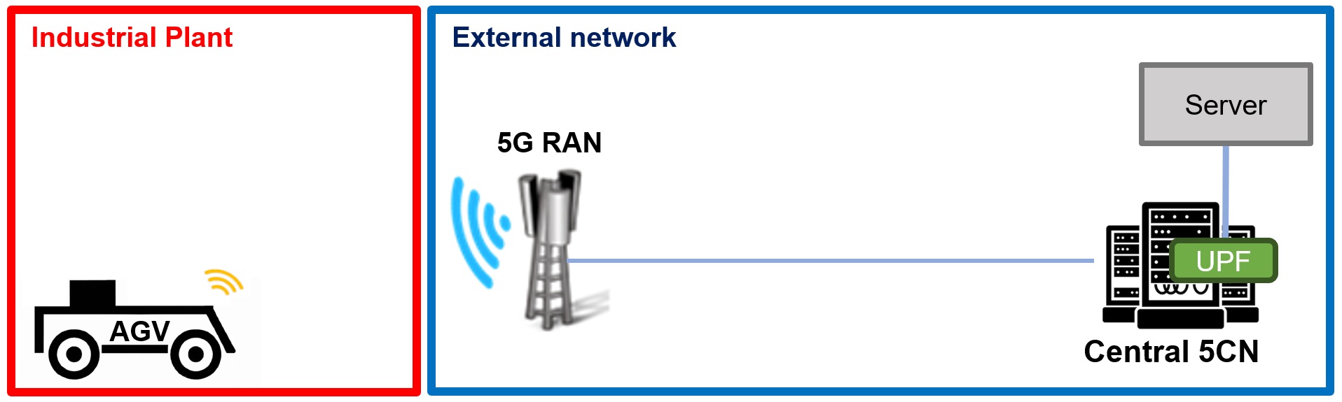
(a) Architecture 1.

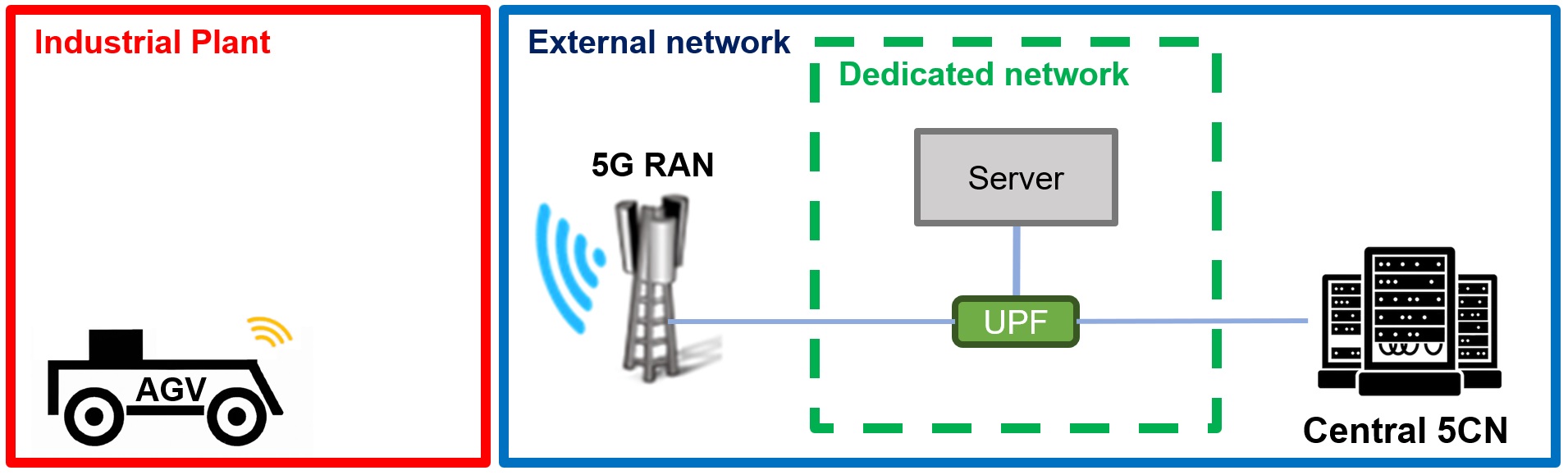
(b) Architecture 2.

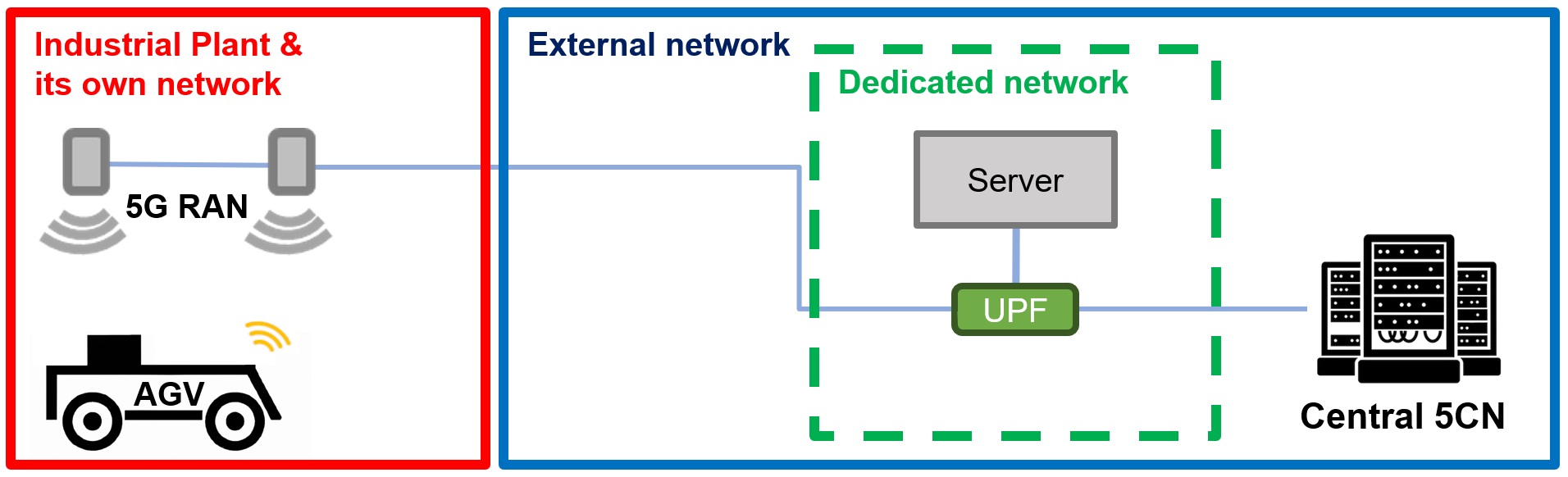
(c) Architecture 3.

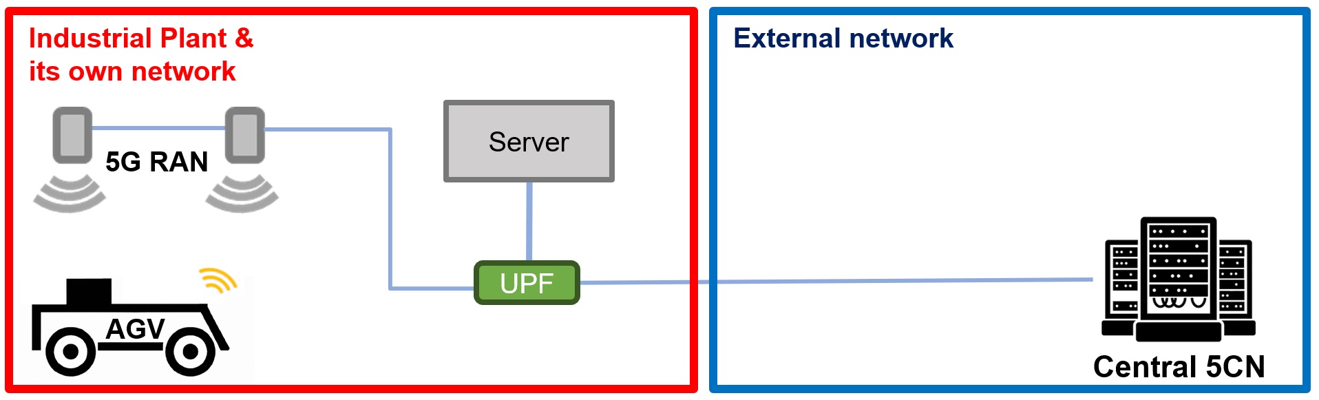
(d) Architecture 4.

Figure 1: Pictorial representation of the considered 5G NR network architectures.

For the scenario described in Sec. I, we foresee four different 5G NR network architectures which are depicted in Fig. 1 and described hereafter.

1. Architecture 1: both the 5G Radio Access Network (RAN) and 5G Core Network (5CN) are deployed outside the factory (see Fig. 1(a));

2. Architecture 2: the application server and User Plane Function (UPF) functionalities are hosted at the network operator’s premises closer to the industrial plant (see Fig. 1(b)), and 5G RAN is deployed outside the factory;

3. Architecture 3: the 5G RAN is deployed in the industrial plant, whereas the application server and UPF functionalities are hosted at the public network operator’s premises (see Fig. 1(c));

4. Architecture 4: the 5G RAN, the application server, and the UPF functionalities are deployed inside the factory, whereas the other 5CN elements are external (see Fig. 1(d)).

In all cases, the 5G RAN is composed of a single gNodeB (gNB). These architectures, proposed by TIM, draw inspiration from the 5G-ACIA documentations [4].

II-B Traffic model

Each UE collects information about the AGV movements (e.g., positions, axial and angular accelerations, etc.) and sends them to the application server with a fixed periodicity $\tau_{\rm UL}$.

Upon receiving each uplink transmission, the server leverages DL to assess whether or not there will be a future fall of the dangerous liquids carried by the considered AGV. With a probability $p_{\rm DL}$, the DL algorithm will predict a future liquid fall. In this case, the server sends a command to the UE to prevent the fall, otherwise, it will not generate any downlink transmission.

II-C Channel Model

The channel model is based on the Gilbert-Elliot model [5]. It is a 2-state Markov model, where the states are usually referred to as good (G) and bad (B). $g$ and $b$ are the probabilities of correct reception when being in state G and B, respectively, such that $g\gg b$. The transition probability from state G to B is $u$, while the transition probability from state B to G is $v$. Therefore, the reception error rate $p_{\rm{e}}$ in steady state is:

$$p_{\rm e}= (1-g)\pi_{\rm G}+(1-b)\pi_{\rm B},$$ (1)

where $\pi_{\rm G}=\frac{v}{u+v}$ and $\pi_{\rm B}=\frac{u}{u+v}$ are the probability of being in state G and B, respectively.

II-D Implementation of the 5G NR framework

In the frequency domain, the available bandwidth $B$ is split in $n_{\rm{RB}}$ Resource Blocks, where each RB is composed of 12 Orthogonal Frequency Division Multiplexing (OFDM) subcarriers, such that:

$$n_{\rm{RB}}= \left\lfloor\frac{B}{12\Delta f}\right\rfloor,$$ (2)

where $\Delta f$ is the Subcarrier Spacing (SCS).

In the time domain, OFDM symbols are grouped into slots, in particular, 14 OFDM symbols form one slot. However, in 5G NR, it is also possible to have communications over fractions of slots, the so-called “mini-slots”. In this regard, we used mini-slots composed of 7 OFDM symbols each.

We consider the same uplink messages defined in [6], with the inclusion of the downlink ones, as summarized in the following:

• Physical Uplink Control Channel (PUCCH), used by UEs to ask the gNB for being scheduled. It occupies 1 RB and 7 OFDM symbols.

• Physical Downlink Control Channel (PDCCH), used by the gNB to inform the UEs about the uplink/downlink scheduling outcome. It occupies 1 RB and 7 OFDM symbols.

• Physical Uplink Shared Channel (PUSCH), used by UEs to transmit Physical (PHY) Protocol Data Units. It occupies 1 or more RB and 4 OFDM symbols depending on the network load, scheduling policy, etc.

• Physical Downlink Shared Channel (PDSCH), used by the gNB to transmit PHY PDUs to UEs. It occupies 1 or more RB and 4 OFDM symbols.

• Hybrid Automatic Repeat reQuest (HARQ) Acknowledgment (ACK), used to inform the sender about the outcome of the uplink/downlink transmission. It occupies 1 RB and 2 OFDM symbols.

It is worth mentioning that a PUSCH/PDSCH transmission is followed by the corresponding HARQ ACK and the overall process has a duration of one mini-slot. Indeed, we assume half-duplex communications, and that one OFDM symbol is needed to switch from transmission to reception and vice-versa.

II-E Implementation of the 5G NR dynamic scheduling

The gNB makes scheduling decisions, i.e., assigns RBs and OFDM symbols to UEs, both in uplink and downlink, every $T_{\rm{SRP}}$. Specifically, $T_{\rm{SRP}}$ is formed by 8 mini-slots, where half are dedicated to the control plane (i.e., PUCCH, PDCCH and HARQ ACKs) and the other half to the data plane (i.e., PUSCH, and PDSCH).

The control plane resource assignment is fixed a-priori, i.e., each UE knows when to transmit/receive PUCCHs/PDCCHs, respectively, according to a predetermined pattern that repeats over time and depends on the number of resources available, as well as network load. On the opposite, the data plane resources are scheduled based on the current traffic needs, according to the 5G NR scheduling mechanisms denoted as dynamic scheduling. In particular, UEs willing to transmit data in the uplink have to first send a PUCCH before receiving the indications via PDCCH on how to transmit the PUSCHs. Additionally, in the downlink, the gNB exploits the PDCCHs to tell the UEs when (and how) they will receive data. To make the scheduling decisions, the gNB exploits the two scheduling policies defined in [6], by applying them independently to the uplink and downlink traffic flows.

III DL-based RUL estimation pipeline

In this section, we describe (i) how we created a dataset from experiments in a real-world industry plant, and (ii) the DL-based pipeline for RUL estimation. It is worth mentioning that some details are omitted due to confidentiality reasons.

III-A Data collection

We performed an experimental campaign where we collected real-time data (accelerations, positions, etc.) of the AGV moving within the industrial pilot line of BIREX. Several sessions were registered, where, during each session, the AGV carried a bottle of water and was forced, at some point in time, to perform a sudden change in its path, thereby leading to the fall of the bottle. A custom script registered the fall event’s timestamp to correctly label the closest sensor’s data as a Fault event and, consequently, all the others were labeled as Non-Fault. The data collected within each session constitute time series data, as they record the AGV movement over time with regular intervals and timestamps, resulting in a sequence of ordered observations. In this context, we formulate the RUL prediction problem as a binary classification task, where the objective is to predict whether a Fault event occurs within a certain margin $m$. This margin defines the classification task since it determines the number $m$ of time series samples prior to a Fault event that can be labeled as Fault and should trigger the server to send a command to the AGV for avoiding potential failures.

III-B Data pre-processing

The real-time data collected by the AGV has been manipulated via different pre-processing steps that are listed hereafter:

• Class weighting [7] to cope with the skewed distribution where the majority of the data points correspond to the normal operating conditions and a minority of the data points correspond to the failed state, as usual in RUL scenarios;

• Feature creation to obtain a more suitable representation of the physical phenomenon. Specifically, we created the mean, maximum, minimum, and standard deviation over multiple fixed-length windows [8], as well as the derivative of those time series as the difference between subsequent data points;

• Differencing to remove seasonality from the time series data [9]. This was done by subtracting from each data point the mean acceleration value for its position and orientation;

• Standardization to ensure that all features are on a similar scale and improve the performance and convergence of DL models during training.

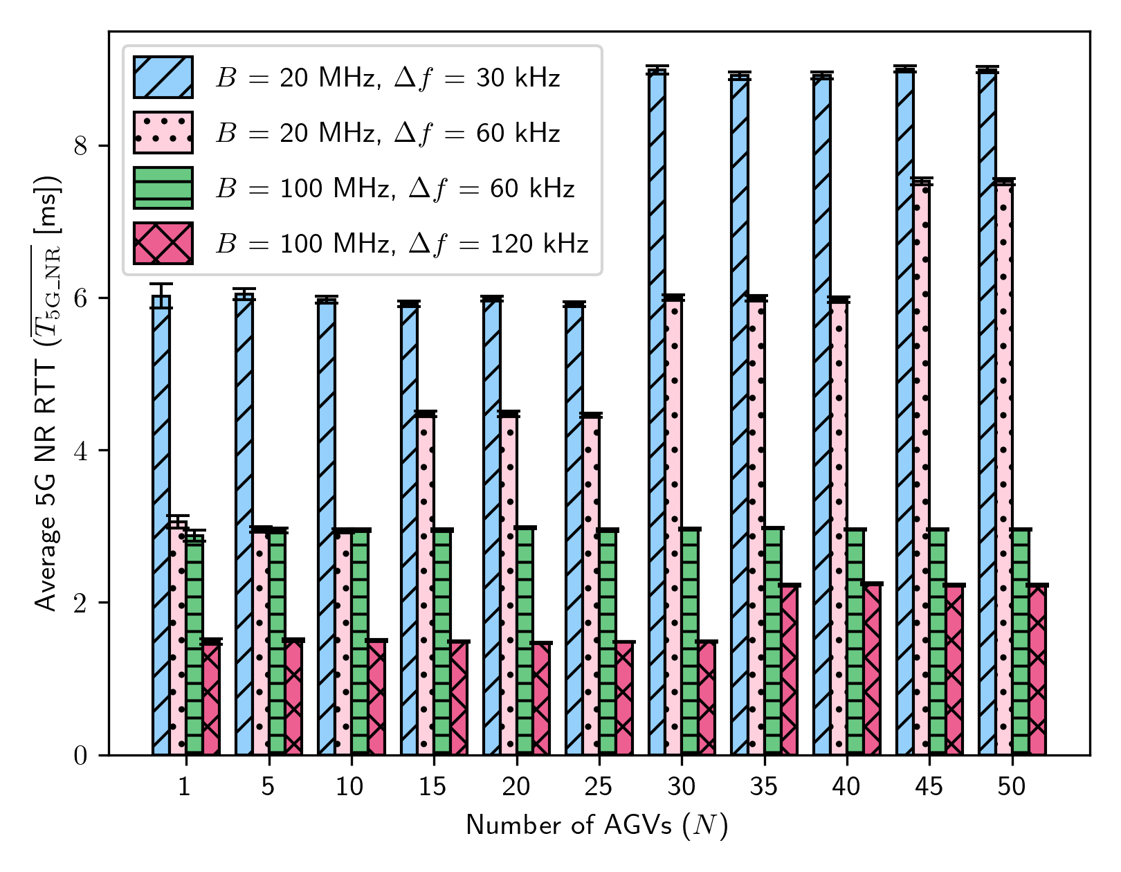
Figure 2: $\overline{T_{\rm{5G\_NR}}}$ as a function of $N$, $B$ and $\Delta f$. We set $M=256$ and $T_{\rm{CN}}=0$ ms.

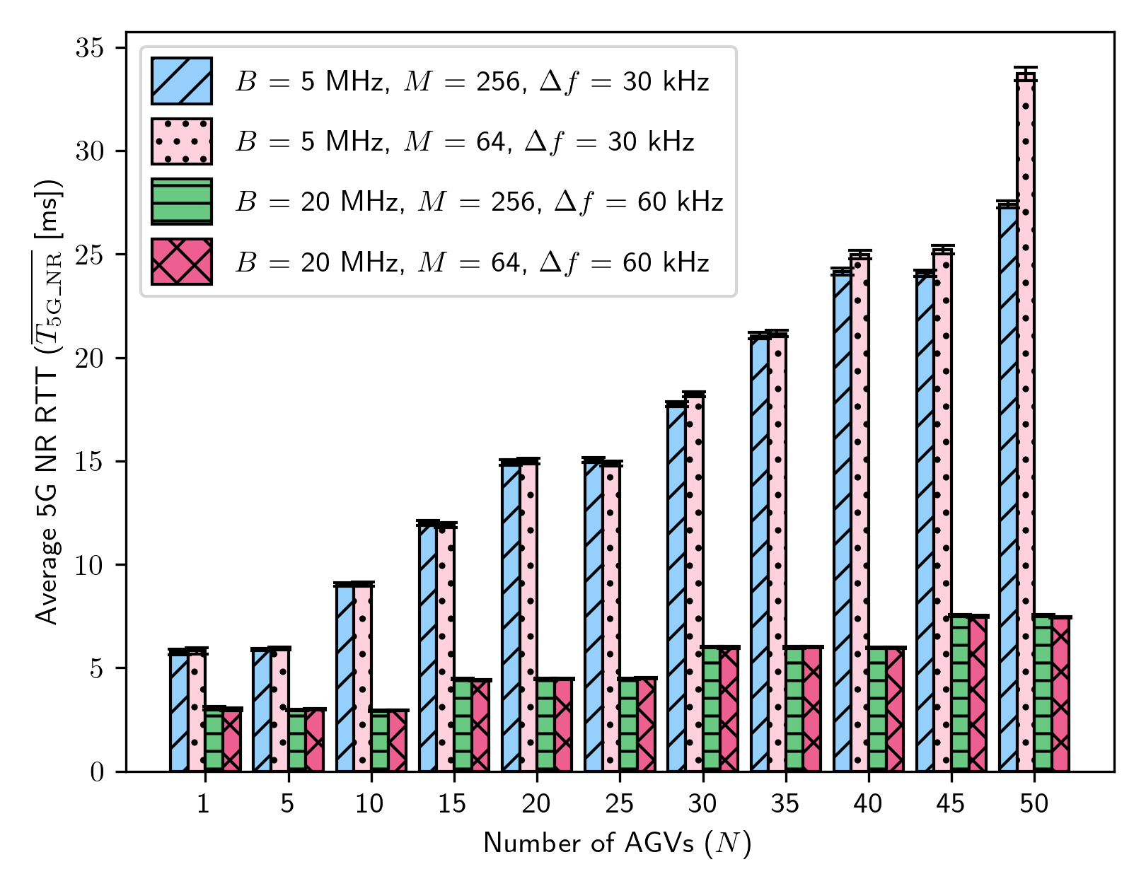
Figure 3: $\overline{T_{\rm{5G\_NR}}}$ as a function of $N$, $B$, $\Delta f$, and $M$. We set $T_{\rm{CN}}=0$ ms.

III-C DL-based pipeline

To perform RUL estimations, the server implements a DL-based pipeline that is formed by a DL model and a threshold-based algorithm. Indeed, the former is trained on the data collected during the hands-on measurement campaign to predict the RUL, and the latter transforms the DL output to either zero or one as the RUL task is tackled as a binary classification problem (see Sec. III-A).

The DL-based pipeline was trained, optimized, and tested by exploiting the manipulated dataset described in Sec. III-B. Specifically, the dataset was further partitioned into 4-folds, i.e., 1) a training set to train the DL model, 2) a validation set to monitor the DL model performance at training time, 3) another validation set to define the optimal value of the threshold, and 4) a test set to evaluate the DL-based pipeline performance.

In particular, the validation set of step 3) is used iteratively in a procedure that aims to find the optimal threshold which minimizes the cost function $C$, whose expression for a DL model $X$ over a set of $K$ time series $S=\{S_{1},S_{2},\ldots,S_{\rm K}\}$ is as follows:

$$C=\sum_{k=1}^{K}\sum_{p=1}^{P_{\rm k}}C_{\rm FP}+\sum_{k=1}^{K}\sum_{q=1}^{Q_{\rm k}}C_{\rm FN}(s_{\rm q},S_{\rm k},m),$$ (3)

where $P_{\rm k}$ is the number of false positive samples for the $k$-th time series, $Q_{\rm k}$ is the number of false negative samples for the $k$-th time series, $C_{\rm FP}$ is the cost for a false positive sample, $C_{\rm FN}$ is the cost for a false negative sample. The expressions for $C_{\rm FP}$ and $C_{\rm FN}$ are the following:

$$\begin{split}C_{\rm FP}&=0.2\\ C_{\rm FN}(s_{\rm q},S_{\rm k},m)&=m-|S_{\rm k}|+q,\end{split}$$ (4)

where $m$ is the margin, $S_{\rm k}$ is a time series, and $q$ is the index of $s_{\rm q}$ in $S_{\rm k}$. We set the cost of false positives $C_{\rm FP}$ constant, regardless of their occurrence in the time series or the margin, while the cost of false negatives $C_{\rm FN}$ increases the closer the sample is to the anomalous event. This design choice is inherently bounded to safety-critical applications, where false negative samples are considered the major risk to deal with.

However, the most important metric to assess the quality of the DL-based pipeline is the average advance function $\bar{a}({D}_{\rm X})$, where ${D}_{\rm X}=\{{s}_{1},{s}_{2},\ldots,{s}_{\rm K}\}$ is the set of the first samples in the time series detected correctly as faulty by a given model $X$ for a given margin $m$. It indicates the amount of time before the actual fault occurs and it is defined as follows:

$$\bar{a}({D}_{\rm X})=\frac{\sum_{i=1}^{K}a({s}_{\rm i})}{K},$$ (5)

where $a({s}_{\rm i})$ is the advance function which indicates the amount of time before the actual fault occurs after sample ${s}_{\rm i}$.

IV Round-Trip Time Analysis

We define the RTT for a single UE as the time from which the movements’ data are generated at the application layer to the time it receives the corresponding command. In particular, its expression is given by:

$$R= T_{\rm{P\_S}}+2\cdot(T_{\rm{P\_gNB}}+T_{\rm{P\_UE}}+T_{\rm{CN}})+T_{\rm{RAN\_UL}}+$$

$$+T_{\rm{RAN\_DL}}+T_{\rm{A}}=$$

$$=T_{\rm{P\_S}}+T_{\rm{5G\_NR}}+T_{\rm{A}},$$ (6)

where:

• $T_{\rm{P\_S}}$ is the processing time of the DL-based pipeline described in Sec. III;

• $T_{\rm{P\_gNB}}$ is the time needed by the gNB to process a PHY PDU, i.e., to eliminate all headers along the 5G protocol stack;

• $T_{\rm{P\_UE}}$ is the time needed by the UE to process a PHY PDU;

• $T_{\rm{CN}}$ is the delay introduced by the 5CN;

• $T_{\rm{RAN\_UL}}$ is the time needed by the UE to successfully perform an uplink transmission;

• $T_{\rm{RAN\_DL}}$ is the time needed by the gNB to successfully perform a downlink transmission;

• $T_{\rm{A}}$ is the time needed to execute the actuation command;

• $T_{\rm{5G\_NR}}$ is the overall delay contribution caused by 5G NR.

We then introduce the term $\overline{T_{\rm{5G\_NR}}}$, as well as the average RTT $\bar{R}$, both averaged among the total number of 5G UEs, i.e., $N$, and the total number of simulations $N_{\rm S}$.

V Numerical results

Parameter	Description	Value
$B$	Overall system bandwidth	{5, 20, 100} MHz
$\Delta f$	Subcarrier spacing	{30, 60, 120} kHz
$M$	Modulation order of	{64, 256}
	PUSCHs/PDSCHs transmissions
$p_{\rm{e}}$	Reception error rate in steady state	$1\%$
$P_{\rm{UL}}$	Uplink payload	32 B
$P_{\rm{DL}}$	Downlink payload	1 B
$p_{\rm DL}$	Downlink generation probability	$10\%$
$T_{\rm{P\_gNB}}$	gNB processing time	7 OFDM symbols
$T_{\rm{P\_UE}}$	UE processing time	7 OFDM symbols
$T_{\rm{CN}}$	Delay introduced by the 5CN	{1, 2, 7} ms
$T_{\rm{SRP}}$	Scheduling periodicity	8 mini-slots
$T_{\rm{S}}$	Simulation time	10 s
$\tau_{\rm{UL}}$	Uplink periodicity	100 ms
$H$	5G protocol stack header	72 B
$N_{\rm S}$	Number of simulations	20

Table I: Simulation parameters

	$m=5$		$m=10$		$m=15$
Model $X$	$C$	$\bar{a}({D}_{\rm X})$	$C$	$\bar{a}({D}_{\rm X})$	$C$	$\bar{a}({D}_{\rm X})$
BASELINE	80.80	0.24s	306.40	0.46s	448.20	1.07s
LR	96.00	0.32s	221.20	0.44s	679.60	0.45s
DDNN	43.40	0.27s	142.00	0.66s	311.20	0.95s
1D-CNN	28.80	0.27s	114.40	0.80s	197.60	1.33s
AE	2396.40	0.39s	2666.80	0.90s	2561.80	1.40s
LSTM	95.40	0.20s	346.40	0.34s	569.80	0.81s
BiLSTM	61.60	0.28s	272.40	0.48s	689.40	1.08s
GRU	85.40	0.23s	290.80	0.68s	539.80	0.92s

Table II: Cost and average advance function of seven DL models and a baseline threshold-based approach for three different margins.

V-A Performance of the 5G NR network

Simulations parameters, if not otherwise specified, are reported in Table I. However, it is important to underline that:

• We assume that $p_{\rm{e}}=1\%$ and $M=\{64,256\}$ for PUSCH and PDSCH communications, but PUCCH, PDCCH and HARQ ACK receptions are error-free as they are transmitted with the most conservative modulation order, i.e., $p_{\rm{e}}=0\%$ due to $M=4$;

• We set $p_{\rm DL}=10\%$ to have, on average, multiple PDSCH transmissions per UE within the simulation time $T_{\rm{S}}$.

• Among the four mini-slots per $T_{\rm{SRP}}$ dedicated to data plane resources (see Sec. II-E), three of them are dedicated to PUSCHs, and only one to PDSCHs, due to the uplink-oriented nature of the considered traffic model (see Sec. II-B);

• All results will show a confidence interval with a probability of $90\%$.

We start the analysis by investigating the impact of different network parameters on the term $T_{\rm{5G\_NR}}$ of Eq. (6), where we set $T_{\rm CN}=0$ ms to be independent of the four architectures defined in Sec. II-A.

In particular, Fig. 3 shows $\overline{T_{\rm{5G\_NR}}}$ as a function of $N$, $B$, $\Delta f$, and by setting $M=256$. It can be observed that a wider bandwidth provides better performance due to a higher number of RBs (see Eq. (2)), for both the control and data plane. Quite interestingly, there is also a benefit when $\Delta f$ increases for a fixed value of $B$. This is because the shorter $T_{\rm{SRP}}$ duration translates into more transmission opportunities per unit of time. As expected, $\bar{R}$ increases with $N$ but exhibits a stepwise behavior. The reason is that, for sufficiently high values of $N$, it is not possible to serve all UEs within one $T_{\rm{SRP}}$ because of a shortage of control plane resources; therefore, some UEs have to transmit/receive their PUCCHs/PDCCHs in the next scheduling periodicity with a consequent non-negligible increase in the average RTT.

To assess the impact of different modulation orders for a different set of bandwidths, Fig. 3 depicts $\overline{T_{\rm{5G\_NR}}}$ as a function of $N$, $B$, $\Delta f$, and by considering $M=64$ and $M=256$. It can be clearly noted that, regardless of the values of $N$, both modulation orders provide the same performance when $B=20$ MHz. This is no longer true in the case of $N\geq 30$ and $B=5$ MHz, where it is preferable to have a higher modulation order, i.e., $M=256$. This is because, otherwise, there is a shortage of data plane resources, and some UEs are forced to transmit/receive their PUSCHs/PDSCHs in the next scheduling periodicity.

V-B Performance of the DL-based RUL estimation pipeline

In this section, we present the performance of the DL-based RUL estimation pipeline that has been constructed, trained, and tested as described in Sec. III.

Specifically, Table II illustrates the cost $C$ and average advance function $\bar{a}({D}_{{\rm X}})$ (see Eqs. (3) and (5)) provided by seven different DL models, including Logistic Regression (LR), Deep Dense Neural Networks (DDNN), Autoencoders (AE), 1D Convolutional Neural Network (1D-CNN), Long Short Term Memory (LSTM), Bi-directional Long Short Term Memory (BiLSTM), Gated Recurrent Unit (GRU) [10, 11, 12], and a baseline threshold-based approach which works over the raw data. Three margins have been considered, that is, $m=\{5,10,15\}$. It can be clearly seen that a trade-off exists for all the considered models, as low margins (i.e., $m=5$) correspond to low average advance and cost, while high margins (i.e., $m=15$) correspond to higher average advance and cost.

However, 1D-CNN is the best-performing model when considering both metrics because it better captures the local temporal patterns present in the data. More complex memory-based models, such as LSTM, BiLSTM and GRU, are not effective in this particular RUL estimation task. This is because only a few input samples are relevant for predicting the liquid fall, whereas recurrent models are designed to capture long-term dependencies and patterns in time series data. Another notable observation is that the reconstruction error, which autoencoders seek to minimize, may not be an effective indicator for predicting the RUL because these models exhibited markedly inferior performance compared to the others.

V-C Performance of the entire RUL chain

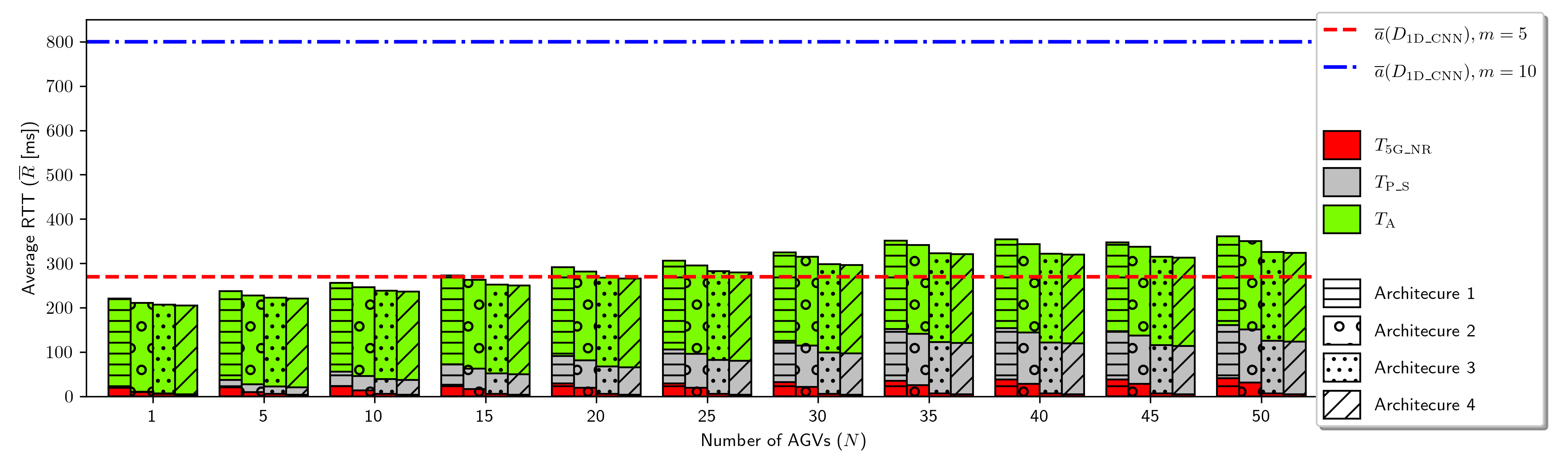
Figure 4: Average RTT $\bar{R}$, as a function of $N$, and the four network architectures described in Sec. II-A, when considering 1D-CNN as DL model, and two average advance values $\bar{a}({D}_{\rm 1D\_CNN})$ for $m=5$ and $m=10$.

In this section, we finally assess whether or not the average RTT provided by the four 5G NR IIoT architectures described in Sec. II-A is sufficiently lower than the average advance provided by 1D-CNN, i.e., the best performing DL model according to the results presented in Sec. V-B. To this aim, we exploited the 5G NR network simulator described in Sec. II by considering the same settings described in Sec. V-A. However, differently from Sec. V-A, this RTT analysis also considers the first and third terms of Eq. (6), as well as the four network architectures described in Sec. II-A. In particular:

• $T_{\rm{P\_S}}$ ranges from $1.2$ ms to $119.2$ ms, depending on the number of UEs. This range derives from experimental tests that consider 1D-CNN processing when considering an i9-11900K processor with 128 GB of RAM and up to 50 parallel flows;

• $T_{\rm A}=200$ ms and is taken from a commercial product.

• Due to their structure, and by leveraging real-world data coming from the TIM infrastructure, we consider that Architecture 1 and 2 work with $B=5$ MHz, $\Delta f=30$ kHz, $M=256$, and are characterized by $T_{\rm{CN}}=7$ ms, and $T_{\rm{CN}}=2$ ms, respectively. Conversely, Architecture 3 and 4 operate with $B=100$ MHz, $\Delta f=120$ kHz, $M=64$, and are characterized by $T_{\rm{CN}}=2$ ms, and $T_{\rm{CN}}=1$ ms, respectively.

As a result, Fig. 4 shows the average RTT, $\bar{R}$, as a function of $N$, and the four network architectures described in Sec. II-A. Average advance values $\bar{a}({D}_{\rm 1D\_CNN})$ for $m=5$ and $m=10$ are represented with dashed horizontal lines. The different colors of each bar represent a diverse delay contribution, that is, $T_{\rm 5G\_NR}$, $T_{\rm P\_S}$, and $T_{\rm A}$ (see Eq. (6)), while different architectures are represented by different bar patterns.

Notably, when $N\leq 10$, all architectures provide an $\bar{R}$ lower than the average advance margin with $m=5$. As expected, Architecture 3 and 4 are the best-performing ones, as they are characterized by higher bandwidths, SCS, and smaller core network delays; indeed, they still yield sufficiently lower average RTTs for $N=15$ and $N=20$. Nevertheless, when $N\geq 25$, it is necessary to change the RUL task by increasing $m$ up to 10, independently of the considered network architectures. However, as described in Sec. V-B, a higher margin leads to an increase in the cost $C$, i.e., the number of erroneous fall predictions, which could compromise the safety conditions within the factory. Finally, it is worth highlighting that the average RTT is mainly affected by application-specific parameters, i.e., $T_{\rm P\_S}$ and $T_{\rm A}$, and optimizations of 5G NR are not really needed for the considered IIoT scenario and settings.

VI Conclusions

In this paper, we performed an E2E analysis of a RUL estimation problem, where all its three main elements, namely application, communication system, and RUL logic, have been studied. In particular, we considered a safety-critical IIoT application where 5G NR is used to collect movements data from AGVs carrying dangerous liquids, while DL algorithms are trained to foresee the potential liquid falls.

The problem is analyzed by considering 4 different 5G NR architectures, 7 DL-based and 1 threshold-based algorithm, as a function of different system parameters. The main findings of this analysis are reported hereafter:

• Wider bandwidths and/or subcarrier spacings lead to lower RTTs, whereas employing higher modulation orders is beneficial only when the data plane resources saturate;

• 1D-CNN is the best-performing DL model for RUL estimation as it shows the best trade-off between cost and average advance for all the considered margins;

• The use of dedicated RAN and 5CN resources, as in Architecture 3 and 4, together with their network settings result in a reduction of the average RTT w.r.t other solutions, like Architecture 2 and 1;

• The training of 1D-CNN for RUL estimation needs a margin $m\geq 10$ to provide an average advance time compatible with the average RTT performance provided by all the considered network architectures;

• The training of 1D-CNN for RUL estimation can leverage a margin $m=5$, which features lower costs, for certain architectures and number of AGVs $N$. However, if the RTT increases, due to an increase of $N$ or to a less performing architecture, using the set up with $m=10$ is required;

• The average RTT is mainly affected by application-specific parameters, i.e., $T_{\rm P\_S}$ and $T_{\rm A}$, rather than 5G NR-related optimizations.

In future works, we aim to address more realistic, and therefore complex, scenarios by considering multiple gNBs and different channel models. Our future research will also target reliability assessment for safety critical RUL-based chains.

References

- [1] C. Ferreira and G. Gonçalves, “Remaining useful life prediction and challenges: A literature review on the use of machine learning methods,” Journal of Manufacturing Systems, vol. 63, pp. 550–562, 2022.
- [2] 3GPP, TR 22.804 - Study on Communication for Automation in Vertical domains (CAV), 7 2020. Rel 16.3.0.
- [3] 3GPP, TR 23.501 - System architecture for the 5G System (5GS), 4 2023. Rel 18.1.0.
- [4] 5G ACIA, 5G Non-Public Networks for Industrial Scenarios, 9 2021.
- [5] G. Hasslinger and O. Hohlfeld, “The Gilbert-Elliott Model for Packet Loss in Real Time Services on the Internet,” in 14th GI/ITG Conference - Measurement, Modelling and Evalutation of Computer and Communication Systems, pp. 1–15, Mar. 2008.
- [6] G. Cuozzo, S. Cavallero, et al., “Enabling URLLC in 5G NR IIoT Networks: A Full-Stack End-to-End Analysis,” in 2022 Joint European Conference on Networks and Communications & 6G Summit (EuCNC/6G Summit), pp. 333–338, 2022. ISSN: 2575-4912.
- [7] G. Haixiang, L. Yijing, et al., “Learning from class-imbalanced data: Review of methods and applications,” Expert Systems with Applications, vol. 73, pp. 220–239, 2017.
- [8] J. Brownlee, Introduction to Time Series Forecasting With Python. Machine Learning Mastery, 2018.
- [9] R. Manuca and R. Savit, “Stationarity and nonstationarity in time series analysis,” Physica D: Nonlinear Phenomena, vol. 99, no. 2, pp. 134–161, 1996.
- [10] H. I. Fawaz, G. Forestier, et al., “Deep learning for time series classification: a review,” Data Mining and Knowledge Discovery, vol. 33, pp. 917–963, mar 2019.
- [11] A. Borghesi, A. Bartolini, et al., “Anomaly detection using autoencoders in high performance computing systems,” Proceedings of the AAAI Conference on Artificial Intelligence, vol. 33, pp. 9428–9433, jul 2019.
- [12] Y. Wu, M. Yuan, et al., “Remaining useful life estimation of engineered systems using vanilla lstm neural networks,” Neurocomputing, vol. 275, pp. 167–179, 2018.