A Semi-Automated Solution Approach Selection Tool for Any Use Case via Scopus and OpenAI: a Case Study for AI/ML in Oncology

Abstract

In today’s vast literature landscape, a manual review is very time-consuming. To address this challenge, this paper proposes a semi-automated tool for solution method review and selection. It caters to researchers, practitioners, and decision-makers while serving as a benchmark for future work. The tool comprises three modules: (1) paper selection and scoring, using a keyword selection scheme to query Scopus API and compute relevancy; (2) solution method extraction in papers utilizing OpenAI API; (3) sensitivity analysis and post-analyzes. It reveals trends, relevant papers, and methods. AI in the oncology case study and several use cases are presented with promising results, comparing the tool to manual ground truth.

[inst1]organization=Department of Materials and Production, Aalborg University,addressline=Fibigerstræde 16, city=Aalborg, postcode=9220, country=Denmark

Automated support for literature choice and solution selection for any use case.

A generalized keyword selection scheme for literature database queries.

Trends in literature: detecting AI methods for a case study using Scopus and OpenAI.

A better understanding of the tool by sensitivity analyses for Scopus and OpenAI.

Robust tool for different domains with promising OpenAI performance results.

1 Introduction

Over the past decade, artificial intelligence (AI) and machine learning (ML) have gained significant attention in the fields of information technology and computer science, accompanying significant advancements and benefits across diverse industries and sectors [1, 2]. There are numerous AI/ML taxonomies presented in the literature that can be used to select a collection of AI strategies to address a specific challenge [3, 4]. Figure 1 illustrates an example taxonomy of the extensive AI/ML domain, encompassing multiple problem types and branches. However, to search for AI methods specific to a given use case, it is not only necessary to select a fitting branch in the taxonomy, but one also has to refine the search by comparing it to the standing knowledge base of the literature on the use case.

The increasing amount of literature presents a challenge for decision-makers seeking to employ AI/ML methodology in their specific problem domains. Manual review is time-consuming [5], often resulting in incomplete information without targeted searches. A tool that rapidly generates trend findings and examines solution methods for any use case would be extremely beneficial in various situations.

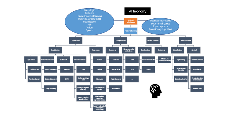
Figure 1: An example of AI/ML taxonomy.

This research proposes a semi-automatic tool developed to generate results on solution approaches for any use case. The study presents results on multiple problem domains on AI with a focus on the case study for AI/ML in oncology. The proposed scheme contains the following steps:

• Determining keywords systematically from the use case by a two-domain, three-level setup.

• Automated literature extraction using selected keywords via Scopus Search API [6].

• Extracting AI methods automatically from Scopus search results by using OpenAI API.

• Sensitivity-analyzes for both Scopus and OpenAI.

• Post-analyzes based on results.

The proposed scheme can be used iteratively for the decision makers to augment their understanding of the problem and similarly align the keywords better with the desired use case and specificity level, consequently obtaining better results.

The remainder of this paper is structured as follows: Sec. 2 reviews the use of AI methods and the literature on model selection approaches. Sec. 3 presents the proposed AI method selection tool, and Sec. 4 showcases the performance, sensitivity, and post-analysis of the method. In Sec. 5, discussion, conclusion, and suggestions for future works are given.

2 Literature review

In the literature, there are reviews and surveys on which AI approaches or applications are used for different problem domains such as building and construction 4.0 [7], architecture, engineering and construction (AEC) [8], agriculture [9], watermarking [10], healthcare [11, 12], oil and gas sector [13], supply chain management [14], pathology [15], banking [16], finance [17], food adulteration detection [18], engineering and manufacturing [19], renewable energy-driven desalination system [20], path planning in UAV swarms [21], military [22], cybersecurity management [23], engineering design [24], vehicular ad-hoc networks [25], dentistry [26], green building [27], e-commerce [28], drug discovery [29], marketing [30], electricity supply chain automation [31], monitoring fetus via ultrasound images [32], IoT security [33].

As can be seen, some of the problem domains in the example review and surveys are low-level, while some are high-level. The abstraction level is difficult to integrate for the solution domain while considering the reviews and surveys. Even if the same problem domain is considered, it will be an issue to depend on reviews or surveys in the literature as there may be an unlimited number of use case scenarios and levels of specificity. In addition, AI approaches specified in reviews or surveys can sometimes be very general. In this case, it may be necessary to make article reviews manually, and it causes labor and time lost [34]. Based on this idea, one can search for an automated way to minimize the time spent on manual review in order to get an AI method applied to a given use case.

The last decade saw significant steps toward a fully automatic model selection scheme with tools that select models for specialized use cases, generally referred to as model determination, parameter estimation, or hyper-parameter selection tools. For forecasting time series in R, the popular forecast package by R. Hyndman et al. was presented, showcasing great initial results [35]. For regression models, the investigated selection procedures are generally based on the evaluation of smaller pre-defined sets of alternative methods, e.g., by information criteria (AIC, BIC), shrinkage methods (Lasso), stepwise regression, and or cross-validation schemes [36]. For ML-based model schemes, the methods proposed by B. Komer et al. [37] introduce the hyperopt package for hyper-parameter selection accompanying the Scikit-learn ML library, J. Snoek et al. [38] presents a bayesian optimization scheme to identify the hyper-parameter configuration efficiently, and J. Bergstra et al. [39] identifies hyper-parameter configurations for training neural networks and deep belief networks by using a random search algorithm and two greedy sequential methods based on the expected improvement criterion. There also exist smaller frameworks, e.g., that of hyper-parameter tuning based on problem features with MATE [40], to model and fit autoregressive-to-anything processes in Java [41], or extensions to general purpose optimization frameworks [42].

On the other hand, Dinter et al. [5] presents a systematic literature review on the automation of systematic literature reviews with a concentration on all systematic literature review procedures as well as natural language processing (NLP) and ML approaches. They stated that the main objective of automating a systematic literature review is to reduce time because human execution is costly, time-consuming, and prone to mistakes. Furthermore, the title and abstract are mostly used as features for several steps in the systematic review process proposed by Kitchenham et al. [43]. Even though our research does not stick to these procedures since our study was not a pure systematic literature review, the title and abstract are included for the OpenAI part. Additionally, they found the majority of systematic literature reviews to be automated using support vector machine (SVM) and Bayesian networks, such as Naive Bayes classifiers, and there appears to be a distinct lack of evidence regarding the effectiveness of deep learning approaches in this regard.

The work of H. Chen et al. [44] produce a written section of relevant background material to a solution approach written in the form of a research paper through a bidirectional encoder representation from transformers (BERT)-based semantic classification model. Similarly, K. Heffernan et al. [45] utilizes a series of machine learning algorithms as automatic classifiers to identify solutions and problems from non-solutions and non-solutions in scientific sentences with good results. These findings suggest that ML-based language models can be utilized in the automation of literature review with success.

Consequently, we have identified literature that explains the procedure of manually and automatically reviewing the literature. We have also identified automated tuning frameworks for different modeling schemes. However, there is a gap in the automatic selection of a solution approach. Our paper aims to investigate and address this gap.

3 Methodology

The proposed methodology has three main modules; see the flowchart in Fig. 2. The first module covers selecting keywords and getting results via Scopus Search. Then the advanced search query returns the results where the fields are explained by Scopus Search Views . In the second module, solution methods that are used for each article are searched using the OpenAI API. In the third module, sensitivity and post-analyzes are performed. The flow indicated by the red dashed line is performed automatically.

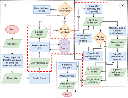
Figure 2: The flowchart shows the proposed methodology where red ellipses are the start and end points, green parallelograms are inputs and outputs, blue rectangles are processes, orange diamonds are decisions, and the purple cylinder is the database. The red dashed line demonstrates the automated flow.

This scheme is appropriate for any problem and solution domain. It can be used for use cases in many different fields. Although the second block of this study focuses on AI methods, this block can also evolve into other topics, such as which hardware to be used and which scientific applications to be employed. However, as the tool relies on the OpenAI framework, ground truth data is created manually to check the performance.

In Tab. 1, the benefits and functions of the methods used in the proposed methodology are shown.

Table 1: Solution method selection comparison table.

Methods / Features	Manual literature review via articles	Manual literature review via surveys and reviews	Proposed method
Reduction of time and effort spent	No	Maybe	Yes
Guaranteeing to search in desired problem and solution detail	Maybe	Maybe	Yes
Automation	No	No	Yes
Making inferences about AI methods utilized for use case (relevancy and popularity)	No	No	Yes

3.1 Module 1: Scopus search

The goal of the first module is to search for a relevant pool of paper w.r.t. the given problem a user is dealing with. To do so, a keyword selection scheme has been made in order to facilitate the user’s work. This scheme is then used to make a Scopus query, but also to score each paper.

To determine keywords, three specification levels (a general, an expended, and a detailed one) are applied to the given problem and the searched solutions. This work is done manually as it involves eliciting user information on the use case. That means both classification and order are specified by the user. However, this stage is critical in recommending more appropriate solution approaches because these keywords are the first inputs to the proposed methodology and determine the pool of papers used in module 2. Fig. 3 gives an example of the proposed keyword selection scheme. Notice that it is possible, but not necessary, to add keywords in each field, where a field refers to the specific level in the block. Leaving some fields empty will lead to a less specified pool of solution approaches, which consequently risks not fitting the use case. At the same time, adding too many keywords can lead either to a too restricted pool of papers (e.g., if one uses too many general keywords, and fulfill each field) or, if too many expanding keywords are given, to a less specific pool of paper as if the field was left empty. The different levels showcase:

• The general and necessary keywords. The keyword must be a part of the research paper for the paper to be in the selected pool of papers.

• The expanding keywords. Here only one of the keywords in the field is necessary for the paper to be selected.

• A further specification. It is only used in the later stage to rank the identified solution methods with the relevancy metric.

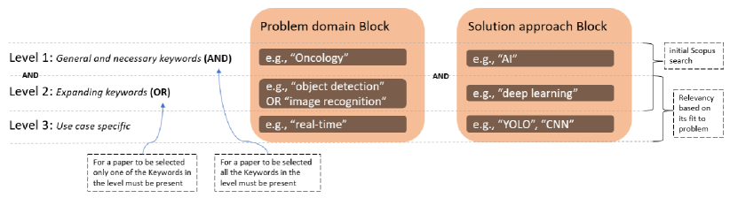
Figure 3: Example illustration of the proposed framework for keyword selection. Note, in the database search, adding some version of a keyword will only search for that specific keyword. Consequently, other versions of that word will also have to be added, but with the logic operator OR to indicate that either version can be used in the paper. E.g. “AI OR artificial intelligence”.

After keyword selection, a query is created for Scopus Search API. Information is searched in titles, abstracts, and keywords of recent articles or conference papers, for the words defined in levels 1 and 2. The query can be, for example:

‘TITLE-ABS-KEY(("oncology") AND ("artificial intelligence" OR "AI")
AND ("image processing")) AND DOCTYPE(ar OR cp) AND PUBYEAR > 2013’

Note that an expert can directly enter a query instead of using the keyword selection scheme. It is useful in some cases, for example: when it is difficult to find a good pool of papers using the query built by the keyword selection scheme, or when one wants to search in a specific field or a specific range of years, or for a first try if one wants to search only for reviews in order to get more appropriate academic keywords. However, it is still advantageous to follow this scheme as it helps to find, classify, and order the use case keywords, but also to specify what is important for scoring the paper.

The publication year, the number of citations, the title, and the abstract information of all articles returned by the Scopus query are saved. After all the results are obtained, the title and abstract information of all the articles are examined manually, and articles that are irrelevant and have not applied/mentioned any AI method are eliminated.

3.2 Module 2: Scoring and method extraction

In this module, the relevancy and popularity metrics for the Scopus search results are computed, and solution methods are extracted from the title and abstract of each paper.

The relevancy metrics count the number of unique level 2 and 3 keywords appearing at least once in the title, abstract, or keywords. Ultimately, the metric represents how well the methods fit the specificity of the use case. For example, a paper named “Hybrid learning method for melanoma detection” yields in the abstract “image recognition (5 times), deep learning (2 times), real-time”; it will therefore have a relevancy metric of 3, taking into account Fig. 3.

The popularity metric is used to know the research interest of a paper and its methods. It is computed by $\frac{\text{citation number}}{\text{publication age in whole years}+1}$ where 1 is added in the denominator to avoid zero divisions.

After calculating the relevancy and popularity metrics, the tool inputs the title and abstract information to OpenAI and outputs the AI approaches used in each article.

When someone provides a text prompt in OpenAI API, the model will produce a text completion that tries to match the context or pattern you provided. Essential GPT-3 models, which generate natural language, are Davinci, Curie, Babbage, and Ada. In this paper, “text-davinci-003” is used which is the most potent GPT-3 model and one of the models that are referred to as “GPT 3.5”. Some issues to consider when preparing prompts are as follows:

• It is advised to place instructions at the start of the prompt and to use ### or ””” to demarcate the context from the instruction.

• Speaking of what to do is preferable to speaking about what not to do.

The prompt can then be the following:

"Extract the names of the artificial intelligence approaches used
from the following text. ###{" + str(document_text) +  "}### \nA:"

where ‘document_text’ includes the title and abstract information of a paper.

To evaluate OpenAI’s performance, the ground truth AI methods are manually produced for non-filtered papers, regarding the title and abstract information of each paper. Some high-level tags, such as “artificial intelligence” and “machine learning” are not included. In other words, the keywords used in Scopus search as a method are not involved. Precision, recall, and F1-measure are calculated for performance analysis.

3.3 Module 3: Analyzes

In this module, sensitivity analyzes are done regarding Scopus and OpenAI. Different combinations of level 1 and 2 keywords in the Scopus query are tried and the initial prompt is compared with other prompts for OpenAI.

For the selected use case, post-analyzes are performed by investigating which AI methods are used more often and which have higher relevancy or popularity metrics and comparing the results over different periods. This can be done manually, or, if there are too many methods listed, first a clustering algorithm can be used to help this investigation. Currently, density-based spatial clustering of applications with noise (DBSCAN) [46] used with ($1-$ the normalized Indel similarity) as distance performs well enough to support post-analysis.

4 Experiments

4.1 Use case definition

The use case example given in Fig. 4 is tackled for our initial experiment. Here, AI is employed on the dataset of images to detect cancer.

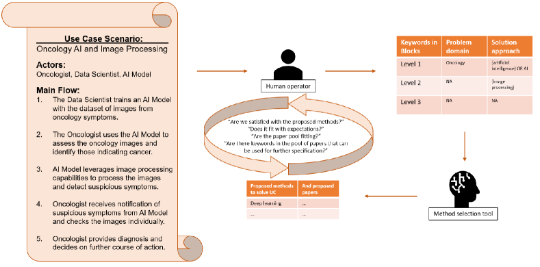
Figure 4: An example use case and an illustration of the procedure of interactively using the proposed method.

4.2 Keywords from the use case scenario

Using Fig. 3, the following keywords are defined: “oncology” as problem level 1, “artificial intelligence” and “AI” as solution level 1. Only “image processing” is used as solution level 2. By using only one level 2 keyword, the experiment stays rather general in the expected results.

For simplicity, level 3 keywords are not used in this example. Level 3 keywords do not affect the pool of papers but enable the user to elicit relevancy to papers that match their use case better. Because the computation of the relevancy metric is trivial, it is omitted in this example.

4.3 Scopus API search and manual article cleaning

According to the selected keywords, our initial query of Scopus API is given below.

‘TITLE-ABS-KEY(("oncology") AND ("artificial intelligence" OR "AI")
AND ("image processing")) AND DOCTYPE(ar OR cp) AND PUBYEAR > 2013’

That means the keywords are searched in the title, abstract, and keyword parts. In addition, to limit the size of the results, the publications published after 2013 are selected, and to be more specific, the document type is restricted to “Article” or “Conference Paper”.

Then DOI, eid, year, and citation number results that Scopus API returns are given in Tab. 5. The relevancy and popularity values are calculated as stated in Sec. 3.2. Currently, some papers can have a relevancy of 0, but by manually checking them, they stay relevant. It happens when keywords only appear in “INDEXTERMS” provided by Scopus but are absent from the title, abstract, and author keywords. Moreover, this is also due to a total absence of keyword level 3. It can be fixed by taking these automatic keywords for the OpenAI analysis.

The query returns 92 results. Among them, 25 publications (irrelevant, not technical, just survey, etc.) indicated in red in Tab. 5 are manually filtered. The remaining 67 articles are the results related to the domains and keywords of the use case. However, there are among them 12 papers, highlighted in orange, that apply an AI method successfully, but they do not mention particular methods (they do only highly general, level 1 and 2 ones) in the title and abstract; they will therefore be missed by the OpenAI extraction part that is stated in Sec. 4.4. However, it is not critical as trends are explored. Still, 55 papers remain to be analyzed. Note that of the 37 articles eliminated, these could have been marked as such if we had implemented the level 3 keywords.

4.4 OpenAI

The initial prompt for the OpenAI API is stated below.

"Extract the names of the artificial intelligence approaches used
from the following text. ###{" + str(document_text) +  "}### \nA:"

where ‘document_text’ includes the title and abstract information of a paper.

After finding methods using OpenAI and manual work, the precision value is calculated. Here it is assumed that manual findings are the actual methods. On the other hand, the results coming from OpenAI are the predicted ones.

4.4.1 OpenAI performance

To analyze the results, the methods found by OpenAI are compared to the ones found by manual investigation (considered ground truths) for each paper. There are four different performance determinants, and they are called

• “true found” the number of methods found both by OpenAI that belong to the ground truths,

• “false found” the number of methods found by OpenAI that do not belong to the ground truths,

• “true general found” the number of methods found by OpenAI and the manual search but belonging to level 1 or 2 keywords or high-level keywords like “machine learning”,

• “total manual” the number of ground truths,

• “missing” = “total manual” - “true found”.

With these data, precision, recall (or sensitivity or true positive rate), and F1-score can be calculated for performance analysis. To do that, the following metrics are employed:

• True Positive (TP) $=$“true found”,

• False Positive (FP) $=$“false found” + “true general found”,

• False Negative (FN) $=$“missing”.

The “true general found” results are counted as False Positive since they are terms that are entered into the Scopus search or they are high-level keywords for our solution domain interest like “machine learning, artificial intelligence-based approach” as mentioned above.

For each paper that is not filtered, the performance metrics are calculated as follows.

• $Precision=TP/(TP+FP)$

• $Recall=TP/(TP+FN)$

• $F1\text{-}score=2\times\frac{Precision\times Recall}{(Precision+Recall)}$

The F1-score assesses the trade-off between precision and recall [47]. When F1-score is high, it indicates that both precision and recall are high. A lower F1-score indicates a larger imbalance in precision and recall.

Let’s check the following example, coming from [48]: “Transfer learning with different modified convolutional neural network models for classifying digital mammograms utilizing Local Dataset”

“ […] accuracy of different machine learning algorithms in diagnostic mammograms […] Image processing included filtering, contrast limited adaptive histogram equalization (CLAHE), then […] Data augmentation was also applied […] Transfer learning of many models trained on the Imagenet dataset was used with fine-tuning. […] NASNetLarge model achieved the highest accuracy […] The least performance was achieved using DenseNet169 and InceptionResNetV2. […]”

Manually, “transfer learning”, “convolutional neural network”, “NASNetLarge”, “DenseNet169”, “InceptionResNetV2”, “data augmentation”, and “fine-tuning” are found as AI methods. What OpenAI has found is highlighted as well. Highlighted in green, “transfer learning”, “convolutional neural network”, “data augmentation”, ‘NASNetLarge”, “DenseNet169” and “InceptionResNetV2” are “true found”; so $TP=6$. Highlighted in orange, “machine learning algorithms” is a “true general found”, and highlighted in red, “contrast limited adaptive histogram equalization (CLAHE)” is “false found”, then $FP=2$. Finally, highlighted in blue “fine-tuning” is a “missing” and so $FN=1$. With these, data can compute $Precision=6/(6+2)=0.75$, $Recall=6/(6+1)=0.86$ and $F1\text{-}score=(2\times 0.75\times 0.86)/(0.75+0.86)=0.8$.

In our studied case (see B), the average scores are good, with an average precision of 0.7111, recall of 0.9226, and F1-score of 0.7775. There are 108 TPs, 51 FPs, and 12 FNs if all 55 results are grouped into a single result pool. The values of the precision, recall, and F1-score are then 0.6793, 0.9, and 0.7742, respectively. All ground truths and OpenAI findings are presented in Tab. 10.

4.5 Sensitivity analyzes

4.5.1 Scopus API sensitivity

For the Scopus sensitivity analysis, different combinations of level 1 keywords are tried in the query. The initial query can be seen in Sec. 4.3.

Table 2: Summary table for different queries, the first query is the initial one, given for comparison.

Query level 1 keywords problem/solution	papers found	common papers with the initial query
“oncology”/ “artificial intelligence” “AI”	92	92
“cancer”/ “artificial intelligence” “AI”	746	64
“oncology”/ “machine learning” “ML”	155	53
{oncology}/ {artificial intelligence} {AI}	92	92
“oncology”/ “artificial intelligence”	89	89
“oncology”/ “AI”	16	16

Tab. 2 shows the impact of changing keywords in level 1. Changing a problem domain keyword with another that could be seen as a synonym can greatly impact the papers found. Using the more specific keyword “machine learning” in the solution domain instead of “artificial intelligence” has an impact on the publications found. Similarly, in the problem domain using “cancer” instead of “oncology” has a great impact on the number of papers found. On the other hand, changing double quotes to braces has not that much effect. Moreover, it seems that using only an abbreviation instead of the open form can change the number of results found. Using only the abbreviation has resulted in a poor paper pool.

However, despite the different pool of papers, the methods found by OpenAI are pretty much the same, both for the second and the third query. This means that using synonyms changes the pool of papers but not the methods used to solve the same kind of problem, which means that the method is robust to the keyword selection scheme.

4.5.2 OpenAI sensitivity

To analyze the sensitivity of OpenAI, different prompts are tested, and the differences of proposed AI methods are checked. Results are summarized in Tab 3, and details are provided in C. The number in the last column is an enriched ratio, meaning that if two prompts are equal, it will obtain an infinite value. However, having a difference between two prompts will lead to a decreasing ratio, considering that two papers do not provide the same set of words but also how many words in the prompt are different.

Below prompts are used for analysis.

"Extract the names of the artificial intelligence approaches used from the following text. ###{" + str(document_text) + "}### \nA:"
Prompt 1
"Just write the names of used artificial intelligence or machine
learning methods in the following text. ###{" + str(document_text) + "}### \nA:"
Prompt 2
"Just write the names of used artificial intelligence methods in the following text. ###{" + str(document_text) + "}### \nA:"
Prompt 3
"Just write the names of the artificial intelligence approaches used in the following text. ###{" + str(document_text) + "}### \nA:"
Prompt 4
"Extract the names of the used artificial intelligence approaches from the following text. ###{" + str(document_text) + "}### \nA:"
Prompt 5
"Write the names of successfully applied artificial intelligence
approaches in the following text. ###{" + str(document_text) + "}### \nA:"
Prompt 6
"Extract the names of the artificial intelligence approaches employed in the following text. ###{" + str(document_text) + "}### \nA:"

Table 3: Summary table for OpenAI sensitivity with respect to the initial prompt.

	Total number of missing / extra or different words	Total number of articles which has the same results	Column 2 divided by column 1
Prompt 1	117	12	0.1026
Prompt 2	107	16	0.1495
Prompt 3	101	15	0.1485
Prompt 4	31	41	1.3226
Prompt 5	96	18	0.1875
Prompt 6	51	34	0.6667

The original prompt has a higher F1-score value than the other six prompts. With these few prompts, it can already be said that OpenAI is sensitive to the sentence used. However, it generally adds words with respect to the manual search, and extracting the most common words belonging to these results should be enough to find what the user is searching for. Moreover, it is observed that changing a word’s position has less impact than changing a word; the more words the user changes, the more differences appear. It also seems that using more common/usual words will give more generic results, closer to the ones that are being searched for; when using very specific instructions, notably in the action verbs, the results will generally be more irrelevant.

4.6 Post-analyzes

The extracted AI methods for the use case described in Sec. 4.1 are presented in D. The total number of appearances of the methods, their relevancy, and popularity metrics are showcased in Tab. 30 by years. Methods selected from articles that are not highlighted in Tab. 5 and appeared at least in two papers are discussed.

Fig. 5 illustrates the summary chart of Tab. 30. It is seen from the figure that many different methods have been investigated to solve our example use case, but some are much more used or popular than others. These methods (e.g., class 2 (deep learning methods) and class 1 (artificial neural networks)) are the ones that the user should investigate in the first place to solve the given use case. To be more specific, until 2018 different types of neural networks, logistic regression, SVM, and random forest are popular methods. After 2018, SVM and neural networks are still utilized, and the extra trees classifier seems popular in 2022. However, the trend is being dominated by deep learning methods. Among the deep learning algorithms, CNN, U-Net, and AlexNet can be counted as the three most used and popular methods.

AI methods can be examined without making any classification, but in this case, there will be too many methods. To simplify this situation, the methods are divided into classes. In D, specifics on method classification and detailed information for AI methods in these classes are provided. Moreover, a more detailed decision-making process can be made by using relevancy and popularity metrics. For example, these metrics support decision-making when being uncertain between two AI methods.

Figure 5: Summary chart of extracted AI methods for “oncology” problem domain and “image processing” solution approach.

4.7 Experiments for different problem domains

In order to check the robustness of the tool, different problem domains and solution approaches are also considered for the Scopus search. The same initial prompt given in Sec. 4.4 is used for all use cases to extract AI methods by utilizing OpenAI API.

First, the same problem domain is kept, and the level 2 solution approach is changed as given in the below query.

‘TITLE-ABS-KEY(("oncology") AND ("artificial intelligence" OR "AI")
AND ("natural language processing" OR "NLP")) AND DOCTYPE(ar OR cp)
AND PUBYEAR > 2013’

The aforementioned search yields 35 documents. Although 5 of them effectively use an AI approach, they do not mention any particular methods in the title or abstract, and 15 of them are irrelevant or merely surveys. Consequently, 15 of them are selected in the manner described in Sec. 4.3. Fig. 6 shows AI methods employed in selected papers. Until 2019, SVM seems to be a popular method, and from 2019 the trend is shifting to deep learning algorithms. Recurrent neural network (RNN), convolutional neural network (CNN), and BERT are among the deep learning methods that are more used after 2019. In addition, some of the most popular methods are BERT, long short-term memory (LSTM), and generative pre-trained transformers (GPT).

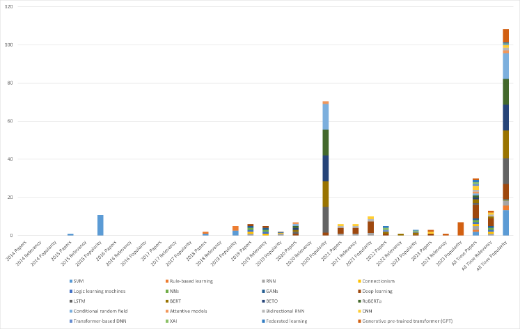
Figure 6: Summary chart of extracted AI methods for “oncology” problem domain and “natural language processing” solution approach.

Secondly, the solution approach components are retained the same while changing the problem domain. The query for the ”traffic control” issue domain is presented below.

‘TITLE-ABS-KEY(("traffic control") AND ("artificial intelligence" OR
"AI") AND ("image processing")) AND DOCTYPE(ar OR cp) AND PUBYEAR
> 2013’

The query returns 52 results, where nine are irrelevant or just surveys, and 20 use an AI method successfully, but they do not mention specific methods in the title and abstract. Therefore, 23 of them are selected. In Fig. 7, it is seen that until 2020, classical methods like scale-invariant feature transform (SIFT), speeded up robust features (SURF), k-nearest neighbors (KNN), and decision trees are popular methods. After 2020, deep learning methods class (that contains region-based CNN (R-CNN), Fast R-CNN, Faster R-CNN, you only look once (YOLO), deep simple online real-time tracking (DeepSORT), CNN, U-Net, etc.) is on the rise in terms of the number of uses and popularity.

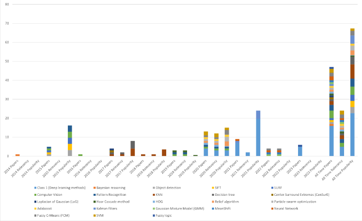
Figure 7: Summary chart of extracted AI methods “traffic control” problem domain “image processing” solution approach.

Another query is the “satellite imagery” for the problem domain, given below. It returns 66 results and 37 of them are selected to be used in analyzes.

‘TITLE-ABS-KEY(("satellite imagery") AND ("artificial intelligence"
OR "AI") AND ("image processing")) AND DOCTYPE(ar OR cp)
AND PUBYEAR > 2013’

Fig. 8 illustrates the summary of extracted AI methods. Class 1 includes CNN, deep neural network (DNN), DeepLabv3+, Fully Convolution Networks (FCN), U-Net, U-Net++, encoder-decoder, attention mechanism, Res2Net, ResNet, LSTM, SegNet, V-Net, U2Net, AttuNet, LinkNet, mask R-CNN, and cloud attention intelligent network (CAI-Net). On the other hand, class 2 covers ant colony optimization (ACO), genetic algorithm, particle swarm optimization (PSO), bat algorithm, and artificial bee colony (ABC). Until 2020, SVM, artificial neural network (ANN), and ACO were frequently used and popular methods. After 2020, the use and popularity of class 1 and PSO appear to be increasing. In class 1, the top three most used and most popular methods are CNN, U-Net, and DNN. As can be seen from the trend, the first methods to be considered in this problem domain may be the deep learning methods given above.

Figure 8: Summary chart of extracted AI methods “satellite imagery” problem domain “image processing” solution approach.

In Tab. 4, OpenAI performance results for all experiments are given, where TP, FP, and FN values are considered as a single pool, i.e., performance metrics are not average values for each article result. It should also be taken into account that if the “true found” words (i.e., machine learning, artificial intelligence, image processing) are not included in the FP, higher precision and F1-score values would have been obtained. Although the problem domain and solution approach change, similar performance results are attained, which is promising for the robustness of the tool.

Table 4: OpenAI performance results for all problem domains.

Problem domain	Solution Approach	Precision	Recall	F1-score
oncology	(artificial intelligence $\vee$ AI) $\wedge$ image processing	0.6793	0.9	0.7742
oncology	(artificial intelligence $\vee$ AI) $\wedge$ (natural language processing $\vee$ NLP)	0.6667	0.9677	0.7895
traffic control	(artificial intelligence $\vee$ AI) $\wedge$ image processing	0.6026	0.9216	0.7287
satellite imagery	(artificial intelligence $\vee$ AI) $\wedge$ image processing	0.7917	0.9406	0.8597

5 Discussion and conclusion

A big issue when utilizing automatic solution method selection schemes is the trust in the fit, relevancy, and popularity of the suggested methods. The fit to the actual use case depends on the ability of the human operator to interact with the tool and whether or not they understand the intricacies of the approach. With the proposed method, the human operator has the ability to validate the suggested methods from the accompanying pool of research papers, and due to the simplicity, responsiveness, and intuitiveness, it is relatively straightforward for the human operator to modify and align the usage of the tool with the overall goal of solving a problem. Additionally, to increase the tool’s performance in terms of operation requirements (e.g., explainability, trustworthiness) and resources (e.g., hardware), the necessary features or extra resources for AI methods can be added and expanded later if the detailed requirements and current resources are stated clearly.

For example, if explainability is required, many different methods exist for obtaining explainable AI (XAI) methods [49, 50, 51, 52, 53, 54]. On the other hand, if trustworthiness is required, then according to the system, environment, goals, and other parameters where AI will be used, several alternative criteria for trustworthiness may be specified [55, 56].

Details or requirements such as explainability and trustworthiness can be retrieved in the keyword selection scheme in Fig. 3. Or, after AI methods are found by the proposed tool, post hoc analyzes can be made with the requirements not used in the proposed method. In some use cases, such requirements or details may not be specified at the beginning of the AI system life cycle and, therefore, may not be included in the keyword selection phase.

Due to the specificity of certain use cases, there is a considerable risk that no research has been conducted on the specifics of the use case. Consequently, the proposed methods will likely not showcase a high score in the relevancy metric. Therefore, the literature pool must be investigated after the results are identified.

Ultimately, the tool’s applicability comes down to the objective of the application. It will comfortably propose methods already explained in the literature as to why it is very useful when identifying trends in the research communities. However, as the method identification is based on historical data that train the tool to determine what words within a research paper can be classified as a method, the tool will not fare well when dealing with entirely new solution approach schemes.

It is noteworthy that the relevancy explained in Sec. 3.2 is computed and saved at the same time as the other data. It could be useful in the future if one wants an automatic filter. On the other hand, if the pool of papers is too big to be manually filtered, it is possible to filter at the end of the process, when one is checking for the methods to be used. The main disadvantage of filtering after the whole process is that it can allow a lot of irrelevant papers to be analyzed by OpenAI, and this will modify the perception of the trends of research for the studied use case. However, note that our tool is used to get trends in research about a given use case to support the selection of solution methods, and does not directly select a method for the user. It means that having some irrelevant papers analyzed in the whole process will not lead to a completely different result. Moreover, no information is lost, so the trends can be recomputed after filtering if necessary.

On the other hand, when the experiments are examined, the tool produces robust results concerning OpenAI performance for different problem and solution domains in its current state. In terms of the trend, up-to-date usage, and popularity of solution methods, our proposed approach quickly produces rich and advantageous information for the user. In addition, the recommended keyword selection scheme offers a very flexible structure in choosing the problem domain and solution approach for any use case.

5.1 Future work

Due to the nature of the underlying problem, certain processes are technically more difficult to automate than others [5]. In its current form, the proposed method still needs a human to perform the keyword selection, check the results given by the query, classify the found methods, and validate the robustness of the solution. For future work, it would be of high value to remove the need for human intervention while presenting results that signify the trade-off for the different automated decisions. Our study towards automating these tasks is currently underway.

Simultaneously, employing versions from the updated suite of large language models, such as OpenAI’s GPT-4, and exploring other databases (like Web of Science, PubMed, IEEE Xplore, etc.) are also future works. Besides, open-source alternatives to GPT-3 or GPT-4, such as GPT-NeoX-20B [57] and GPT-J [58], will be implemented to help in cutting costs.

The sensitivity analysis is split into two parts: queries and prompts. Queries highly depend on the keyword selection scheme and should be studied together. However, reasonably an automatic sensitivity analysis can be made using some variants of the initial query, like using quotation marks instead of brackets or using several forms of the same words. Later, it could be interesting to study the sensitivity concerning synonyms. On the other part, prompts can be analyzed more easily. Indeed, several sentences could be automatically generated with respect to the initial one and then tested. The common pool of solutions, or using a scoring-like number of occurrences, could be a robust amicable solution.

Classifying methods is not easy as we want to keep a stratification level from general methods to specific ones. However, as deep learning is already used to classify images, e.g., gaining attention in cancer research [59], a deep learning method could pool different methods together and reduce the number of methods used like YOLO-v2, YOLOv4-tiny, etc. Without any logical pooling, a simple clustering approach based on the text, such as DBSCAN, can be used to make an automatic pooling for a sufficiently big set of methods extracted. However, if we want to automatically match a specific taxonomy, another method will be needed.

Currently, the tool only checks the title, abstract, and keywords for the method determination. For certain papers, the specifics of the method are only introduced later in the paper. E.g., for hybrid methods. Consequentially, an important extension will be to determine the applied method of a paper from the entirety of a paper.

Finally, the tool can essentially investigate any arbitrary characteristic of the literature rather than only the solution approaches — E.g., identifying problem formulations and varieties therein. Therefore, exploring how to do this manually will greatly benefit the research community.

CRediT authorship contribution statement

Deniz Kenan Kılıç: Conceptualization, Methodology, Software, Validation, Formal analysis, Investigation, Data curation, Writing – original draft, Writing – review & editing, Visualization. Alex Elkjær Vasegaard: Conceptualization, Methodology, Software, Validation, Formal analysis, Investigation, Data curation, Writing – original draft, Writing – review & editing, Visualization. Aurélien Desoeuvres: Conceptualization, Methodology, Software, Validation, Formal analysis, Investigation, Data curation, Writing – original draft, Writing – review & editing. Peter Nielsen: Conceptualization, Methodology, Validation, Investigation, Data curation, Writing – review & editing, Supervision.

Declaration of competing interest

The authors declare that they have no known competing financial interests or personal relationships that could have appeared to influence the work reported in this paper.

Appendix A Scopus and OpenAI results

In Tab. 5, Scopus results are shown for the initial query stated in Sec. 4.3. As it is mentioned, articles highlighted in red are manually deleted, and the orange ones that use the AI method are related to the use case but do not specify it in the title and abstract.

Table 5: Journals regarding Scopus API search (red articles are manually filtered, and orange ones apply an AI method successfully, but they do not mention methods in the title and abstract) where C., R., and P. stand for citation number, relevancy value, and popularity value respectively.

doi	eid	Year	C.	R.	P.
10.3233/978-1-61499-474-9-244	2-s2.0- 84918834255	2014	6	0	0.6
[HTML]FFC000 10.1109/CSCI.2014.26	2-s2.0- 84902660528	2014	3	1	0.3
10.1117/12.2043516	2-s2.0- 84902106481	2014	8	0	0.8
[HTML]FFC000 10.1016/j.compbiomed.2013.11.002	2-s2.0- 84891153909	2014	67	0	6.7
10.1109/ICCICCT.2014.6993162	2-s2.0- 84921642433	2014	27	1	2.7
10.1016/j.procs.2015.07.555	2-s2.0- 84948392681	2015	6	0	0.6667
10.1007/978-3-319-19387-8_204	2-s2.0- 84944318438	2015	9	1	1
10.1088/1742-6596/633/1/012079	2-s2.0- 84983425726	2015	4	0	0.4444
10.1109/CLEI.2015.7360029	2-s2.0- 84961903068	2015	10	0	1.1111
10.1117/12.2216973	2-s2.0- 84988890309	2016	17	1	2.125
[HTML]FFC000 10.1117/12.2208620	2-s2.0- 84981719831	2016	21	0	2.625
[HTML]FF0000	2-s2.0- 84960402804	2016	0	1	0
[HTML]FFC000 10.1089/tmj.2014.0249	2-s2.0- 84954436777	2016	13	0	1.625
[HTML]FF0000 10.1109/TIPTEKNO.2015.7374612	2-s2.0- 84964265510	2016	0	1	0
10.1109/IC4.2015.7375719	2-s2.0- 84962792167	2016	9	0	1.125
10.1109/INDICON.2015.7443447	2-s2.0- 84994285804	2016	14	0	1.75
10.1109/TMI.2015.2506270	2-s2.0- 84963804529	2016	48	0	6
10.1088/0031-9155/61/13/4855	2-s2.0- 84976426664	2016	33	0	4.1250
[HTML]FFC000	2-s2.0- 85038823793	2017	4	1	0.5714

Table 6: Cont.

doi	eid	Year	C.	R.	P.
[HTML]FF0000 10.1016/j.procs.2017.06.122	2-s2.0- 85028633382	2017	23	0	3.2857
[HTML]FFC000 10.1007/978-3-319-60699-6_79	2-s2.0- 85021253325	2017	12	0	1.7143
[HTML]FF0000 10.1109/INTECH.2016.7845044	2-s2.0- 85015305877	2017	8	0	1.1429
10.1109/IPAS.2016.7880148	2-s2.0- 85018542177	2017	19	0	2.7143
[HTML]FFC000 10.1109/C-CODE.2017.7918949	2-s2.0- 85020287797	2017	64	0	9.1429
[HTML]FF0000 10.1093/jnci/djx055	2-s2.0- 85021849026	2017	91	0	13
10.1016/j.ijmedinf.2017.05.016	2-s2.0- 85019985302	2017	23	0	3.2857
10.1109/INTERCON.2017.8079674	2-s2.0- 85039989899	2017	8	1	1.1429
10.1109/IDAP.2017.8090211	2-s2.0- 85039912655	2017	5	1	0.7143
[HTML]FFC000 10.4081/ejh.2017.2838	2-s2.0- 85036544923	2017	10	0	1.4286
10.1109/ICMLC.2017.8107759	2-s2.0- 85042474953	2017	2	1	0.2857
[HTML]FF0000	2-s2.0- 85103213412	2018	0	1	0
[HTML]FF0000 10.1109/TMI.2018.2800298	2-s2.0- 85042927927	2018	60	0	10
10.1109/ICECCO.2017.8333341	2-s2.0- 85050502789	2018	12	1	2
10.1002/cnm.2953	2-s2.0- 85042181700	2018	24	0	4
10.1109/CICN.2018.8864942	2-s2.0- 85074209854	2018	0	1	0
10.1016/j.knosys.2018.05.016	2-s2.0- 85048760650	2018	25	1	4.1667
10.1109/CSCI.2017.72	2-s2.0- 85060645376	2018	0	0	0
10.1007/978-3-030-05532-5_42	2-s2.0- 85059759729	2019	6	1	1.2
[HTML]FF0000 10.1007/s40291-018-0366-4	2-s2.0- 85056306068	2019	15	1	3
[HTML]FF0000 10.1007/s40291-018-0367-3	2-s2.0- 85055963110	2019	6	1	1.2

Table 7: Cont.

doi	eid	Year	C.	R.	P.
[HTML]FFC000 10.1016/j.artmed.2018.09.003	2-s2.0- 85054192769	2019	29	0	5.8
[HTML]FFC000 10.1109/BIBE.2019.00181	2-s2.0- 85077975055	2019	4	1	0.8
10.1016/j.canrad.2019.08.005	2-s2.0- 85073726145	2019	1	0	0.2
10.1109/ACCESS.2020.3028248	2-s2.0- 85099879408	2020	15	1	3.75
	2-s2.0- 85091193990	2020	0	1	0
[HTML]FF0000	2-s2.0- 85086354606	2020	2	1	0.5
10.1117/12.2542161	2-s2.0- 85081629940	2020	0	1	0
[HTML]FF0000 10.1002/mp.13891	2-s2.0- 85075297765	2020	50	0	12.5
10.1145/3374135.3385327	2-s2.0- 85086182046	2020	1	1	0.25
10.1111/cas.14377	2-s2.0- 85082062276	2020	82	0	20.5
10.3892/ijo.2020.5063	2-s2.0- 85084500870	2020	29	0	7.25
10.3390/cancers12113080	2-s2.0- 85093943094	2020	18	0	4.5
10.1109/WCSP52459.2021.9613447	2-s2.0- 85123369429	2021	0	1	0
10.1109/ISPCC53510.2021.9609516	2-s2.0- 85123014841	2021	5	1	1.6667
10.1155/2021/9998379	2-s2.0- 85107175102	2021	14	0	4.6667
[HTML]FFC000 10.3791/61895	2-s2.0- 85138248078	2021	8	1	2.6667
10.1109/JBHI.2020.3003475	2-s2.0- 85096782074	2021	11	0	3.6667
[HTML]FF0000 10.1016/j.ejmp.2021.03.009	2-s2.0- 85102886091	2021	55	1	18.3333
[HTML]FF0000 10.1088/1361-6560/abd4f7	2-s2.0- 85103515923	2021	23	0	7.6667
[HTML]FF0000 10.1016/j.xjtc.2021.03.016	2-s2.0- 85103937126	2021	22	0	7.3333
[HTML]FF0000 10.1038/s41416-021-01386-x	2-s2.0- 85104847620	2021	26	0	8.6667

Table 8: Cont.

doi	eid	Year	C.	R.	P.
10.2217/fon-2020-0987	2-s2.0- 85108124165	2021	2	0	0.6667
[HTML]FF0000 10.3390/jimaging7080124	2-s2.0- 85111942180	2021	2	1	0.6667
10.1093/jrr/rrab070	2-s2.0- 85116348283	2021	7	0	2.3333
[HTML]FF0000 10.1515/cdbme-2021-2057	2-s2.0- 85121865792	2021	2	0	0.6667
10.1109/GCAT52182.2021.9587838	2-s2.0- 85119477680	2021	1	1	0.3333
[HTML]FF0000 10.1148/rg.2021210037	2-s2.0- 85117052739	2021	67	0	22.3333
[HTML]FF0000 10.1016/j.radi.2021.07.012	2-s2.0- 85114341702	2021	10	0	3.3333
[HTML]FF0000 10.1002/onco.13862	2-s2.0- 85111119804	2021	2	0	0.6667
[HTML]FF0000 10.1007/s11018-022-02003-w	2-s2.0- 85124348701	2021	1	0	0.3333
10.1155/2022/2259373	2-s2.0- 85135422352	2022	0	1	0
10.1016/j.ebiom.2021.103757	2-s2.0- 85121330341	2022	17	0	8.5
10.1371/journal.pone.0264140	2-s2.0- 85125337919	2022	4	0	2
10.1007/s11042-022-12067-z	2-s2.0- 85124261031	2022	3	0	1.5
[HTML]FF0000 10.1053/j.sult.2022.02.005	2-s2.0- 85125529381	2022	4	1	2
[HTML]FF0000 10.3145/epi.2022.jul.08	2-s2.0- 85137378624	2022	0	1	0
10.3390/ijerph19159057	2-s2.0- 85135382796	2022	4	0	2
[HTML]FF0000 10.1007/s00261-021-03254-x	2-s2.0- 85113512614	2022	20	0	10
10.1007/s13534-022-00227-x	2-s2.0- 85131873486	2022	0	0	0
10.1111/exsy.12938	2-s2.0- 85124549532	2022	3	1	1.5
[HTML]FFC000 10.2967/jnumed.122.264063	2-s2.0- 85139515590	2022	3	0	1.5
10.1186/s13014-022-02102-6	2-s2.0- 85134588716	2022	2	0	1

Table 9: Cont.

doi	eid	Year	C.	R.	P.
10.1109/ATEE58038.2023.10108394	2-s2.0- 85159074452	2023	0	0	0
	2-s2.0- 85148402129	2023	0	1	0
10.3390/ijms24021554	2-s2.0- 85146500215	2023	0	0	0
10.3390/s23020926	2-s2.0- 85146428707	2023	0	0	0
10.1109/JTEHM.2022.3224021	2-s2.0- 85144032371	2023	0	0	0
10.1007/s11042-022-13046-0	2-s2.0- 85131537962	2023	2	0	2
10.3390/s23073548	2-s2.0- 85152350497	2023	0	0	0
10.1016/j.bspc.2023.104647	2-s2.0- 85147848611	2023	1	1	1
[HTML]FF0000 10.1016/j.ciresp.2022.10.023	2-s2.0- 85144536545	2023	0	1	0
10.1016/j.bspc.2023.104729	2-s2.0- 85148874931	2023	0	1	0

In Tab. 10, OpenAI results for the initial prompt and ground truth methods extracted manually are shown with performance determinants. These performance determinants are utilized to calculate performance metrics stated in 4.4.1.

Table 10: OpenAI and manually found results for used AI methods in each article.

eid	Methods (OpenAI)	Methods (Manual)	Performance Determinants
2-s2.0- 84918834255	Paraconsistent Artificial Neural Network (PANN)	Paraconsistent Artificial Neural Network (PANN)	Total manual: 1 True found: 1 False found: 0 Missing: 0 True general found: 0

Table 11: Cont.

eid	Methods (OpenAI)	Methods (Manual)	Performance Determinants
2-s2.0- 84902106481	Kernel-based metric, Hilbert-Schmidt independence criterion (HSIC), reproducing kernel Hilbert space (RKHS), k-nearest- neighbor (k-NN) classifier	Hilbert-Schmidt independence criterion (HSIC), reproducing kernel Hilbert space (RKHS), k-nearest- neighbor (k-NN) classifier	Total manual: 3 Total found: 3 False found: 1 Missing:0 True general found: 0
2-s2.0- 84921642433	Artificial Neural Network, Genetic Algorithm	Artificial Neural Network, genetic algorithm	Total manual: 2 True found: 2 False found: 0 Missing: 0 True general found: 0
2-s2.0- 84948392681	Connected Component Labelling, K-Means, Morphological Filter	Connected component labelling, K-means, morphological filter	Total manual: 3 True found: 3 False found: 0 Missing: 0 True general found: 0
2-s2.0- 84944318438	Artificial Neural Networks	Artificial neural networks	Total manual: 1 True found: 1 False found: 0 Missing: 0 True general found: 0
2-s2.0- 84983425726	Probabilistic Neural Network Classifier, Dull Razor algorithm, Level Sets, Automated Thresholding Approach	Dull Razor algorithm, Probabilistic Neural Network Classifier	Total manual: 2 True found: 2 False found: 2 Missing: 0 True general found: 0
2-s2.0- 84961903068	Support Vector Machine	Support Vector Machine	Total manual: 1 True found: 1 False found: 0 Missing: 0 True general found: 0
2-s2.0- 84988890309	Machine learning, Image processing, Random Forests, Sparse Coding	Random Forests, Sparse Coding, SIFT	Total manual: 3 True found: 2 False found: 0 Missing: 1 True general found: 2
2-s2.0- 84962792167	Supervised classification, Multi-Layer Feed- forward Neural Network, Genetically Optimized Fuzzy C-means clustering	Multi-Layer Feed- forward Neural Network, Genetically optimized Fuzzy C-means clustering	Total manual: 2 True found: 2 False found: 0 Missing: 0 True general found: 1

Table 12: Cont.

eid	Methods (OpenAI)	Methods (Manual)	Performance Determinants
2-s2.0- 84994285804	Support Vector Machine (SVM), Sequential Minimal Optimization (SMO)	Support Vector Machine (SVM), Sequential Minimal Optimization (SMO)	Total manual: 2 True found: 2 False found: 0 Missing: 0 True general found: 0
2-s2.0- 84963804529	Artificial Neural Networks, Logistic Regression, LIPU	Artificial Neural Networks, Logistic regression, Logistic regression using Initial variables and Product Units (LIPU)	Total manual: 3 True found: 3 False found: 0 Missing: 0 True general found: 0
2-s2.0- 84976426664	Supervised Machine Learning, Decision Trees	Decision tree	Total manual: 1 True found: 1 False found: 0 Missing: 0 True general found: 1
2-s2.0- 85018542177	Neural Network based classification, Shape Characterization, Color and Texture Features	Neural network classifier, semantic analysis	Total manual: 2 True found: 1 False found: 2 Missing: 1 True general found: 0
2-s2.0- 85019985302	Probabilistic Neural Network (PNN), Exhaustive Search, Features Selection, Leave-one-out(LOO), External Cross-validation (ECV)	Probabilistic Neural Network (PNN) classifier, leave-one-out (LOO), external cross- validation (ECV)	Total manual: 3 True found: 3 False found: 2 Missing: 0 True general found: 0
2-s2.0- 85039989899	Neural Networks	Neural networks	Total manual: 1 True found: 1 False found: 0 Missing: 0 True general found: 0
2-s2.0- 85039912655	Artificial Neural Network Learning Algorithm	Artificial Neural Network	Total manual: 1 True found: 1 False found: 0 Missing: 0 True general found: 1
2-s2.0- 85042474953	Pattern recognition, Adaptive thresholding, Morphological operators, Texture features, Color features	Pattern recognition, Adaptive thresholding	Total manual: 2 True found: 2 False found: 3 Missing: 0 True general found: 0

Table 13: Cont.

eid	Methods (OpenAI)	Methods (Manual)	Performance Determinants
2-s2.0- 85050502789	Machine Learning, k-Nearest Neighbors	k-Nearest Neighbors algorithm	Total manual: 1 True found: 1 False found: 0 Missing: 0 True general found: 1
2-s2.0- 85042181700	Support Vector Machine, Random Forest, Neural Network, Fast Discriminative Mixed-Membership–Based Naive Bayesian Classifiers	Support vector machine, random forest, neural network, fast discriminative mixed-membership–based naive Bayesian classifiers information theory	Total manual: 5 True found: 4 False found: 0 Missing: 1 True general found: 0
2-s2.0- 85074209854	GLCM, SVM	SVM, GLCM Note: Grey Level Co- Occurence Matrix	Total manual: 2 True found: 2 False found: 0 Missing: 0 True general found: 0
2-s2.0- 85048760650	Machine Learning, Digital Image Processing, Feature Selection	Decision tree	Total manual: 1 True found: 0 False found: 1 Missing: 1 True general found: 2
2-s2.0- 85060645376	Gabor filtering, Local Mesh Patterns	Gabor filtering, Local Mesh Patterns	Total manual: 2 True found: 2 False found: 0 Missing: 0 True general found: 0
2-s2.0- 85059759729	Machine learning algorithms, Support Vector Machines	Support vector machines	Total manual: 1 True found: 1 False found: 0 Missing: 0 True general found: 1
2-s2.0- 85073726145	Connectionism, Logics, Neural Networks, General Adversial Networks, Deep Learning	Neural network, General adversial networks, deep learning	Total manual: 3 True found: 3 False found: 2 Missing: 0 True general found: 0
2-s2.0- 85099879408	Perceptron, Color Local Binary Patterns, Color Histograms of Oriented Gradients, Generative Adversarial Network, ABCD Rule, ResNet, AlexNet, Back-Propagation Perceptron	Neural network, perceptron, generative adversarial network, ResNet, AlexNet, back-propagation perceptron	Total manual: 6 True found: 5 False found: 3 Missing: 1 True general found: 0

Table 14: Cont.

eid	Methods (OpenAI)	Methods (Manual)	Performance Determinants
2-s2.0- 85091193990	Artificial Intelligence, Deep Learning	Deep Learning	Total manual: 1 True found: 1 False found: 0 Missing: 0 True general found: 1
2-s2.0- 85081629940	Support Vector Machines	Support vector machines	Total manual: 1 True found: 1 False found: 0 Missing: 0 True general found: 0
2-s2.0- 85086182046	Computer Vision, Clustering, Neural Networks	Computer Vision, Clustering, Neural Networks	Total manual: 3 True found: 3 False found: 0 Missing: 0 True general found: 0
2-s2.0- 85082062276	Deep Learning	Deep learning	Total manual: 1 True found: 1 False found: 0 Missing: 0 True general found: 0
2-s2.0- 85084500870	Deep learning	Deep learning	Total manual: 1 True found: 1 False found: 0 Missing: 0 True general found: 0
2-s2.0- 85093943094	Machine Learning, Linear Discriminant Analysis	Linear Discriminant Analysis	Total manual: 1 True found: 1 False found: 0 Missing: 0 True general found: 1
2-s2.0- 85123369429	U-Net, Deep Learning, Image Segmentation, Artificial Intelligence	U-Net, Deep learning	Total manual: 2 True found: 2 False found: 0 Missing: 0 True general found: 2
2-s2.0- 85123014841		CNN	Total manual: 1 True found: 0 False found: 0 Missing: 1 True general found: 0

Table 15: Cont.

eid	Methods (OpenAI)	Methods (Manual)	Performance Determinants
2-s2.0- 85107175102	Artificial Neural Network (ANNs), Local Binary Pattern (LBP), Gray Level Co-occurrence Matrix (GLCM), Convolutional Neural Network (CNNs), AlexNet, ResNet50	Deep learning, active contour method, Local Binary Pattern (LBP), Gray Level Co-occurrence Matrix (GLCM), artificial neural network (ANNs), convolutional neural network (CNNs), AlexNet, ResNet50	Total manual: 8 True found: 6 False found: 0 Missing: 2 True general found: 0
2-s2.0- 85096782074	Deep learning, Image registration, Deep learning- based nucleus detection	Deep learning, Image registration	Total manual: 2 True found: 2 False found: 1 Missing: 0 True general found: 0
2-s2.0- 85108124165	Deep Learning, Artificial Intelligence Machine Learning	Deep learning	Total manual: 1 True found: 1 False found: 0 Missing: 0 True general found: 2
2-s2.0- 85116348283	2D U-Net, 3-D U-Net	2D U-Net, 3-D U-Net	Total manual: 2 True found: 2 False found: 2 Missing: 0 True general found: 0
2-s2.0- 85119477680	SVM, KNN, Ensemble Learning	SVM, KNN, Ensemble Learning	Total manual: 3 True found: 3 False found: 0 Missing: 0 True general found: 0
2-s2.0- 85135422352	OTSU threshold segmentation, artificial intelligence algorithms	OTSU	Total manual: 1 True found: 1 False found: 0 Missing: 0 True general found: 1
2-s2.0- 85121330341	Extra Trees Classifier, Machine Learning	Extra Trees Classifier	Total manual: 1 True found: 1 False found: 0 Missing: 0 True general found: 1
2-s2.0- 85125337919	Convolutional Neural Network (CNN) algorithms	Convolutional neural network (CNN)	Total manual: 1 True found: 1 False found: 0 Missing: 0 True general found: 0

Table 16: Cont.

eid	Methods (OpenAI)	Methods (Manual)	Performance Determinants
2-s2.0- 85124261031	Fully Connected Networks (FCNs) and U-Net	U-Net, full connected networks (FCNs), U-Net++	Total manual: 3 True found: 2 False found: 0 Missing: 1 True general found: 0
2-s2.0- 85135382796	Deep learning, auto-segmentation	Deep learning	Total manual: 1 True found: 1 False found: 1 Missing: 0 True general found: 0
2-s2.0- 85131873486	Deep Learning, Convolution algorithm	Deep learning Convolution algorithm	Total manual: 2 True found: 2 False found: 0 Missing: 0 True general found: 0
2-s2.0- 85124549532	Deep Learning (DL) Broad Learning System (BLS) Incremental Learning Algorithm	Deep learning, incremental learning algorithm	Total manual: 2 True found: 2 False found: 1 Missing: 0 True general found: 0
2-s2.0- 85134588716	Deep Reinforcement Learning, Deep Image-to-Image Network (DI2IN), Convolutional Encoder-Decoder Architecture, Multi-Level Feature Concatenation	Deep reinforcement learning, convolutional encoder-decoder architecture, multi-level feature concatenation	Total manual: 3 True found: 3 False found: 1 Missing: 0 True general found: 0
2-s2.0- 85159074452	Deep Convolutional Neural Networks, Fusion of the decision of several neural networks, Horizontal Voting	Deep convolutional neural networks, horizontal voting ensemble	Total manual: 2 True found: 2 False found: 1 Missing: 0 True general found: 0
2-s2.0- 85148402129	Transfer learning, Convolutional Neural Networks, Machine Learning Algorithms, Contrast Limited Adaptive Histogram Equalization (CLAHE), Data Augmentation, NASNetLarge, DenseNet169, InceptionResNetV2	Transfer learning, convolutional neural network, NASNetLarge, DenseNet169, InceptionResNetV2, data augmentation, fine tuning	Total manual: 7 True found: 6 False found: 1 Missing: 1 True general found: 1
2-s2.0- 85146500215	Neural Networks, Deep Learning	Neural network, deep learning	Total manual: 2 True found: 2 False found: 0 Missing: 0 True general found: 0

Table 17: Cont.

eid	Methods (OpenAI)	Methods (Manual)	Performance Determinants
2-s2.0- 85146428707	Artificial Intelligence (AI), Convolutional Neural Network (CNN), Intraclass Clustering	Convolutional neural network (CNN), Intraclass Clustering	Total manual: 2 True found: 2 False found: 0 Missing: 0 True general found: 1
2-s2.0- 85144032371	Unsupervised Learning, K-means Clustering, Algorithm, Deep Learning	Deep learning, K-means clustering	Total manual: 2 True found: 2 False found: 0 Missing: 0 True general found: 1
2-s2.0- 85131537962	Artificial Intelligence, Deep Learning, Conditional Generative Adversarial Network (cGAN)	Conditional Generative Adversarial Network (cGAN), generative deep learning	Total manual: 2 True found: 2 False found: 0 Missing: 0 True general found: 1
2-s2.0- 85147848611	Ant Colony Optimization, Sine Cosine Strategy, Disperse Foraging Strategy, Specular Reflection Learning Strategy, Non-Local Mean Strategy, 2D Kapur’s Entropy Strategy	Ant colony optimization	Total manual: 1 True found: 1 False found: 5 Missing: 0 True general found: 0
2-s2.0- 85148874931	Artificial Intelligence, Deep Learning Machine Learning	Deep learning	Total manual: 1 True found: 1 False found: 0 Missing: 0 True general found: 2

Appendix B OpenAI performance results

Below, OpenAI performance results for 55 articles are listed in the same order as Tab. 10.

• TP = [1, 3, 2, 3, 1, 2, 1, 2, 2, 2, 3, 1, 1, 3, 1, 1, 2, 1, 4, 2, 0, 2, 1, 3, 5, 1, 1, 3, 1, 1, 1, 2, 0, 6, 2, 1, 2, 3, 1, 1, 1 ,2, 1, 2, 2, 3, 2, 6, 2, 2, 2, 4, 2, 1, 1]

• FP = [0, 1, 0, 0, 0, 2, 0, 2, 1, 0, 0, 1, 2, 2, 0, 1, 3, 1, 0, 0, 3, 0, 1, 2, 3, 1, 0, 0, 0, 0, 1, 2, 0, 0, 1, 2, 0, 0, 1, 1, 0, 0, 1, 0, 1, 1, 1, 2, 0, 1, 1, 1, 1, 5, 2]

• FN = [0, 0, 0, 0, 0, 0, 0, 1, 0, 0, 0, 0, 1, 0, 0, 0, 0, 0, 1, 0, 1, 0, 0, 0, 1, 0, 0, 0, 0, 0, 0, 0, 1, 2, 0, 0, 0, 0, 0, 0 ,0, 1, 0, 0, 0, 0, 0, 1, 0, 0, 0, 2, 0, 0, 0]

• Precisions = [1, 0.75, 1, 1, 1, 0.5 ,1, 0.5, 0.6667, 1, 1, 0.5, 0.3334, 0.6, 1, 0.5, 0.4, 0.5, 1, 1, 0, 1, 0.5, 0.6, 0.625, 0.5, 1, 1, 1, 1, 0.5, 0.5, 0, 1, 0.6667, 0.3334, 1, 1, 0.5, 0.5, 1, 1, 0.5, 1, 0.6667, 0.75, 0.6667, 0.75, 1, 0.6667, 0.6667, 0.8, 0.6667, 0.1667, 0.3334] and Average(Precisions) = 0.7111

• Recalls = [1, 1, 1, 1, 1, 1, 1, 0.6667, 1, 1, 1, 1, 0.5, 1, 1, 1, 1, 1, 0.8, 1, 0, 1, 1, 1, 0.8334, 1, 1, 1, 1, 1, 1, 1, 0, 0.75, 1, 1, 1, 1, 1, 1, 1, 0.6667, 1, 1, 1, 1, 1, 0.8571, 1, 1, 1, 0.6667, 1, 1, 1] and Average(Recalls) = 0.9226

• F1-score = [1, 0.8571, 1, 1, 1, 0.6667, 1, 0.5714, 0.8, 1, 1, 0.6667, 0.4, 0.75, 1, 0.6667, 0.5714, 0.6667, 0.8889, 1, 0, 1, 0.6667, 0.75, 0.7143, 0.6667, 1, 1, 1, 1, 0.6667, 0.6667, 0, 0.8571, 0.8, 0.5, 1, 1, 0.6667, 0.6667, 1, 0.8, 0.6667, 1, 0.8, 0.8571, 0.8, 0.8, 1, 0.8, 0.8, 0.7273, 0.8, 0.2857, 0.5] and Average(F1-score) = 0.7775

If all 55 results are considered as a single result pool, then there are 108 TPs, 51 FPs, and 12 FNs. Then precision, recall and F1-score values are 0.6793, 0.9, and 0.7742, respectively.

When the performance metrics are examined, the OpenAI presents good performance for the manually generated ground truths.

Appendix C OpenAI sensitivity results

In Tab. 18, Tab. 22 and Tab. 26, missing and extra/different methods are given with respect to the initial prompt. If there is no missing or extra/different method name, it is expressed by “X”.

Table 18: Missing and extra/different methods for prompts 1 and 2 regarding the initial prompt results.

	Prompt 1		Prompt 2
eid	Missing	Extra or different	Missing	Extra or different
2-s2.0- 84918834255	X	X	X	X
2-s2.0- 84902106481	X	X	X	quantitative ultrasound (QUS), radiofrequency (RF) signals, Euclidean distance
2-s2.0- 84921642433	X	Digital Image processing, GLCM, RGB color feature	X	X
2-s2.0- 84948392681	X	Segmentation, Filtering	X	Segmentation, Filtering, Learning and Non-Learning Methods
2-s2.0- 84944318438	X	Image processing	X	Image processing
2-s2.0- 84983425726	X	Exhaustive search, Leave one out method, GPU card (GeForce 580GTX), CUDA programming framework, C++ programming language	X	Exhaustive search, Leave one out method, CUDA programming framework, C++ programming language
2-s2.0- 84961903068	X	Preprocessing, Segmentation, Feature Extraction, Classification	X	Preprocessing, Segmentation, Feature Extraction, Classification
2-s2.0- 84988890309	Sparse Coding	Pre-processing, Segmentation, Classification, SIFT, Hue, Opponent Angle Histograms, RGB Intensities, Dictionary Learning	Sparse Coding	Pre-processing, Segmentation, Classification, SIFT, Hue, Opponent Angle Histograms, RGB Intensities, Dictionary Learning
2-s2.0- 84962792167	X	Optimized Fuzzy Clustering, Machine Learning	X	Optimized Fuzzy Clustering
2-s2.0- 84994285804	X	Iterative Dilation Method, Feature Vector, SVM Classifier	X	Iterative Dilation Method, SVM Classifier
2-s2.0- 84963804529	X	X	LIPU	Machine Learning, Ordinal Classification
2-s2.0- 84976426664	X	Dice Similarity Coefficient (DSC)	X	Dice Similarity Coefficient (DSC)
2-s2.0- 85018542177	X	Feature Extraction	X	Feature Extraction, ABCD Rule, 7-Point Checklist, Menzies Method, CASH Algorithm
2-s2.0- 85019985302	X	X	X	X
2-s2.0- 85039989899	X	Image Processing, Computer Vision	X	Image Processing

Table 19: Cont.

	Prompt 1		Prompt 2
eid	Missing	Extra or different	Missing	Extra or different
2-s2.0- 85039912655	X	Image Processing Software, Artificial Neural Network Learning Algorithm	X	Image Processing Software, Artificial Neural Network Learning Algorithm
2-s2.0- 85042474953	X	X	X	X
2-s2.0- 85050502789	X	Feature selection, Sequential backward selection, Image processing, Segmentation	X	Image Processing, Feature Extraction, Segmentation, Sequential Backward Selection
2-s2.0- 85042181700	X	Multistage Illumination Compensation, Multimode Segmentation, Information Theory	X	Multistage Illumination Compensation, Multimode Segmentation
2-s2.0- 85074209854	X	Dull-Razor, Image Processing, Automatic Segmentation, Basic Statistical Method	X	Dull-Razor, Image Processing, Automatic Segmentation, Basic Statistical Method
2-s2.0- 85048760650	X	Decision Tree	X	Decision Tree
2-s2.0- 85060645376	X	Statistical estimation	X	Statistical estimation
2-s2.0- 85059759729	X	Image processing techniques	X	Image Processing Techniques
2-s2.0- 85073726145	X	Natural Language Processing, Radiomics	X	Deduction, Induction, Abduction, Radiomics, Natural Language Processing
2-s2.0- 85081629940	X	Cross-Validation, Power Spectral Densities, Gray-Level Co-Occurrence Matrices, Holdout Validation, Stratified Cross-Validation	X	Cross-Validation, Image Processing, Artificial Intelligence
2-s2.0- 85091193990	X	Neural Network Architecture	Artificial Intelligence	X
2-s2.0- 85099879408	X	X	X	X
2-s2.0- 85086182046	X	Artificial Intelligence, Image Processing	X	X
2-s2.0- 85082062276	X	AI, feature extraction	X	X
2-s2.0- 85084500870	X	Radiogenomics, Precision Medicine, Computational Medical Imaging, Molecular Expression	X	X
2-s2.0- 85093943094	X	Receiver-Operating -Characteristic (ROC), Tumor-to-Brain Ratios (TBRmean, TBRmax)	X	Receiver-Operating -Characteristic (ROC) curve

Table 20: Cont.

	Prompt 1		Prompt 2
eid	Missing	Extra or different	Missing	Extra or different
2-s2.0- 85123369429	Image, Segmentation	Path Direct Connection, Dropout Direct Connection, Conv Direct Connection, Constant Scale	Image, Segmentation	Path Direct Connection, Dropout Direct Connection, Conv Direct Connection, Constant Scale
2-s2.0- 85107175102	X	Deep Learning, Transfer Learning	X	Deep Learning
2-s2.0- 85123014841	X	CNN	X	CNN
2-s2.0- 85096782074	X	tissue-type classification algorithm, nucleus detection, immunohistochemistry (IHC)	X	tissue-type classification algorithm, nucleus detection, immunohistochemistry (IHC)
2-s2.0- 85108124165	X	X	X	X
2-s2.0- 85116348283	X	Dice similarity coefficient (DSC), Hausdorff distance (HD)	X	Dice similarity coefficient (DSC), Hausdorff distance (HD)
2-s2.0- 85119477680	X	X	X	Machine Learning
2-s2.0- 85135422352	X	CT Image Processing	X	X
2-s2.0- 85121330341	X	Bidimensional Segmentation, Radiomic Features, Dimensionality Reduction, Class Balancing, 10-fold Cross-Validation, McNemar’s Test	X	Bidimensional Segmentation, Dimensionality Reduction, Class Balancing, 10-fold Cross-Validation, McNemar’s Test
2-s2.0- 85125337919	X	Deep Learning, Receiver Operating Characteristic (ROC), Fivefold Cross-Validation	X	Receiver Operating Characteristic (ROC), Area Under the Receiver Operating Characteristic (AUROC)
2-s2.0- 85124261031	X	U-Net++, Jaccard index	X	U-Net++, Loss Function
2-s2.0- 85135382796	X	Dice similarity coefficient (DSC), Hausdorff distance transform (DT)	X	Dice similarity coefficient (DSC), 95% Hausdorff distance transform (DT)
2-s2.0- 85131873486	X	TMR algorithm, frame- based contrast-enhanced T1-weighted MR images, synthetic CT (sCT), mean absolute error (MAE)	X	TMR algorithm, Synthetic CT (sCT), Convolution with rCT (Conv-rCT) plan, Convolution with sCT (Conv-sCT) plan, Mean Absolute Error (MAE)
2-s2.0- 85124549532	X	X	X	X

Table 21: Cont.

	Prompt 1		Prompt 2
eid	Missing	Extra or different	Missing	Extra or different
2-s2.0- 85134588716	Deep Image -to-Image Network (DI2IN)	Dice Similarity Coefficient (DSC), Hausdorff Distance (HD95)	Deep Image -to-Image Network (DI2IN)	Dice Similarity Coefficient (DSC), Hausdorff Distance (HD95)
2-s2.0- 85144032371	X	Artificial Intelligence	X	X
2-s2.0- 85146428707	X	X	X	X
2-s2.0- 85146500215	X	Patternnet, DICOM, MATLAB	X	Patternnet, MATLAB
2-s2.0- 85148402129	Machine Learning Algorithms	Keras, Python	Machine Learning Algorithms	X
2-s2.0- 85159074452	X	X	X	X
2-s2.0- 85131537962	Artificial Intelligence, Deep Learning, EfficientNets, Artificial Neural Network, Majority Soft Voting	X	Artificial Intelligence, Deep Learning	Transfer Learning, Image Data, Handcrafted Lesion Features, Metadata
2-s2.0- 85152350497	X	Computer Vision	X	X
2-s2.0- 85147848611	X	X	X	X
2-s2.0- 85148874931	Artificial Intelligence	Image processing techniques, Wavelet transform	Artificial Intelligence	Image processing techniques, Wavelet transform

Table 22: Missing and extra/different methods for prompts 3 and 4 regarding the initial prompt results.

	Prompt 3		Prompt 4
eid	Missing	Extra or different	Missing	Extra or different
2-s2.0- 84918834255	X	Artifical Neural Network	X	X
2-s2.0- 84902106481	X	X	X	X
2-s2.0- 84921642433	X	X	X	X
2-s2.0- 84948392681	X	Segmentation, Filtering, Localization, Learning, Non-Learning, ABCD Characteristics	X	X
2-s2.0- 84944318438	X	Image processing	X	Image processing
2-s2.0- 84983425726	X	CUDA programming framework, C++ programming language	X	X
2-s2.0- 84961903068	X	Preprocessing, Segmentation, Feature Extraction, Classification	X	X
2-s2.0- 84988890309	Sparse Coding	Pre-processing, Segmentation, Classification, SIFT, Hue, Opponent Angle Histograms, RGB Intensities, Dictionary Learning	X	X
2-s2.0- 84962792167	X	Supervised learning	Supervised classification	X
2-s2.0- 84994285804	X	Iterative Dilation Method, Illumination Compensation	X	X
2-s2.0- 84963804529	LIPU	Machine Learning, Ordinal Classification	X	X
2-s2.0- 84976426664	X	Predictive Modelling	X	X
2-s2.0- 85018542177	X	Feature Extraction	Shape Characterization, Color and Texture Features	Feature Extraction
2-s2.0- 85019985302	X	X	X	X
2-s2.0- 85039989899	X	Image Processing, Computer Vision	X	X
2-s2.0- 85039912655	X	Image Processing Software, Learning Program	X	X
2-s2.0- 85042474953	X	X	X	X

Table 23: Cont.

	Prompt 3		Prompt 4
eid	Missing	Extra or different	Missing	Extra or different
2-s2.0- 85050502789	X	Feature selection, Sequential backward selection, Image processing, Feature Extraction	X	Image Processing, Feature Extraction, Segmentation, Sequential Backward Selection, Feature Selection
2-s2.0- 85042181700	Support Vector Machine, Random Forest, Neural Network, Fast Discriminative Mixed- Membership– Based Naive Bayesian Classifiers	X	X	X
2-s2.0- 85074209854	X	Dull-Razor software, Image Processing, Automatic Segmentation, Basic Statistical Method	X	X
2-s2.0- 85048760650	X	Decision Tree	X	X
2-s2.0- 85060645376	X	Statistical estimation	X	X
2-s2.0- 85059759729	X	Image Processing	X	image processing techniques
2-s2.0- 85073726145	Deep Learning	Natural Language Processing, Logics-based Systems	X	Deduction, Induction, Abduction, Radiomics, Natural Language Processing, Logics Based Systems
2-s2.0- 85081629940	X	Cross-Validation, Image Processing, Artificial Intelligence	X	Artificial Intelligence
2-s2.0- 85091193990	Artificical Intelligence	X	X	X
2-s2.0- 85099879408	X	X	X	X
2-s2.0- 85086182046	X	X	X	X
2-s2.0- 85082062276	X	AI, Machine Learning	X	AI
2-s2.0- 85084500870	X	Machine learning, Natural language processing, Computer vision	X	X
2-s2.0- 85093943094	X	Receiver-Operating -Characteristic (ROC) curve	X	X

Table 24: Cont.

	Prompt 3		Prompt 4
eid	Missing	Extra or different	Missing	Extra or different
2-s2.0- 85123369429	Image Segmentation	Path Direct Connection, Dropout Direct Connection, Conv Direct Connection, Constant Scale	Image Segmentation	Artifical Intelligence
2-s2.0- 85107175102	X	Deep Learning	X	Deep Learning
2-s2.0- 85123014841	X	CNN, Image Processing, Segmentation	X	X
2-s2.0- 85096782074	X	tissue-type classification algorithm, nucleus detection	X	tissue-type classification algorithm, immunohistochemistry (IHC)
2-s2.0- 85108124165	X	X	X	X
2-s2.0- 85116348283	X	X	X	X
2-s2.0- 85119477680	X	X	X	X
2-s2.0- 85135422352	X	X	X	X
2-s2.0- 85121330341	X	Bidimensional Segmentation, Dimensionality Reduction	X	X
2-s2.0- 85125337919	X	Deep Learning, Receiver Operating Characteristic (ROC), Fivefold Cross-Validation	X	Deep Learning, Receiver Operating Characteristic (ROC)
2-s2.0- 85124261031	X	U-Net++	U-Net	U-Net++
2-s2.0- 85135382796	X	Computed Tomography (CT), Dice similarity coefficient (DSC), Hausdorff distance transform (DT)	X	X
2-s2.0- 85131873486	X	Frame-based contrast- enhanced T1-weighted MR images, synthetic CT (sCT)	X	X
2-s2.0- 85124549532	X	X	X	X
2-s2.0- 85134588716	Deep Image -to-Image Network (DI2IN)	Dice Similarity Coefficient (DSC), Hausdorff Distance (HD95)	X	X
2-s2.0- 85144032371	X	X	X	X
2-s2.0- 85146428707	X	X	X	X
2-s2.0- 85146500215	X	Patternnet, MATLAB	X	X
2-s2.0- 85148402129	Machine Learning Algorithms	X	X	X

Table 25: Cont.

	Prompt 3		Prompt 4
eid	Missing	Extra or different	Missing	Extra or different
2-s2.0- 85159074452	X	X	X	X
2-s2.0- 85131537962	Artificial Intelligence	Transfer Learning, Image Data, Handcrafted Lesion Features, Patient -Centric Metadata, Multi-Input Single-Output (MISO) Model, Evaluation Metrics	Artificial Intelligence, Deep Learning	Transfer Learning
2-s2.0- 85152350497	X	X	X	X
2-s2.0- 85147848611	X	X	X	X
2-s2.0- 85148874931	Artificial Intelligence	Image processing techniques, Wavelet transform	X	X

Table 26: Missing and extra/different methods for prompts 5 and 6 regarding the initial prompt results.

	Prompt 5		Prompt 6
eid	Missing	Extra or different	Missing	Extra or different
2-s2.0- 84918834255	X	X	X	X
2-s2.0- 84902106481	X	X	X	X
2-s2.0- 84921642433	X	X	X	X
2-s2.0- 84948392681	X	Segmentation, Filtering, Localization, Learning, Non-Learning	X	X
2-s2.0- 84944318438	X	Image processing	X	X
2-s2.0- 84983425726	X	CUDA programming framework, C++ programming language	X	X
2-s2.0- 84961903068	X	Preprocessing, Segmentation, Feature Extraction, Classification	X	X
2-s2.0- 84988890309	Sparse Coding	Pre-processing, Segmentation, Classification, SIFT, Hue, Opponent Angle Histograms, RGB Intensities, Dictionary Learning	X	SIFT, Hue, Opponent Angle Histograms, RGB Intensities
2-s2.0- 84962792167	X	X	Supervised classification, Multi-Layer Feed-forward Neural Network, Genetically Optimized Fuzzy C-means clustering	X
2-s2.0- 84994285804	X	Iterative Dilation, Illumination Compensation, Feature Vector	X	Iterative Dilation Method
2-s2.0- 84963804529	X	Machine Learning	X	X
2-s2.0- 84976426664	X	Dice Similarity Coefficient (DSC)	X	Predictive Modelling
2-s2.0- 85018542177	X	Feature Extraction	X	X
2-s2.0- 85019985302	X	X	X	X
2-s2.0- 85039989899	X	Image Processing, Computer Vision	X	Image Processing
2-s2.0- 85039912655	X	Image Processing Software, Learning Program	X	Image Processing Software, Learning Program
2-s2.0- 85042474953	X	X	X	X

Table 27: Cont.

	Prompt 5		Prompt 6
eid	Missing	Extra or different	Missing	Extra or different
2-s2.0- 85050502789	X	Segmentation, Sequential backward selection, Image processing, Feature Extraction	X	Image Processing
2-s2.0- 85042181700	X	X	Support Vector Machine, Random Forest, Neural Network, Fast Discriminative Mixed- Membership– Based Naive Bayesian Classifiers	X
2-s2.0- 85074209854	X	Dull-Razor software, Image Processing, Automatic Segmentation, Basic Statistical Method	X	X
2-s2.0- 85048760650	X	Decision Tree	X	Decision Tree
2-s2.0- 85060645376	X	Statistical estimation	X	X
2-s2.0- 85059759729	X	Image Processing Techniques	X	Image Processing
2-s2.0- 85073726145	X	Natural Language Processing, Logics-based Systems	X	Deduction, Induction, Abduction, Radiomics, Natural Language Processing, Logics Based Systems
2-s2.0- 85081629940	X	Cross-Validation, Image Processing, Artificial Intelligence	X	X
2-s2.0- 85091193990	X	Image Processing	X	Deep Neural Network
2-s2.0- 85099879408	X	X	X	X
2-s2.0- 85086182046	X	X	X	X
2-s2.0- 85082062276	X	X	X	X
2-s2.0- 85084500870	X	Convolutional Neural Networks (CNNs), Generative Adversarial Networks (GANs), Recurrent Neural Networks (RNNs)	X	X
2-s2.0- 85093943094	X	Receiver-Operating -Characteristic (ROC) curve	X	X

Table 28: Cont.

	Prompt 5		Prompt 6
eid	Missing	Extra or different	Missing	Extra or different
2-s2.0- 85123369429	Image Segmentation	Path Direct Connection, Dropout Direct Connection, Conv Direct Connection, Constant Scale	Image Segmentation	Path Direct Connection, Dropout Direct Connection, Conv Direct Connection, Constant Scale
2-s2.0- 85107175102	X	Deep Learning	X	X
2-s2.0- 85123014841	X	X	X	X
2-s2.0- 85096782074	X	tissue-type classification algorithm, nucleus detection, Computational pathology	X	tissue-type classification algorithm, nucleus detection, immunohistochemistry (IHC)
2-s2.0- 85108124165	X	X	X	X
2-s2.0- 85116348283	X	Dice similarity coefficient (DSC), Hausdorff distance (HD)	X	X
2-s2.0- 85119477680	X	X	X	X
2-s2.0- 85135422352	X	Lymph Node Recognition Algorithm	X	X
2-s2.0- 85121330341	X	Bidimensional Segmentation, Radiomic Features, Dimensionality Reduction, Class Balancing, 10-Fold Cross-Validation, McNemar’s Test	X	X
2-s2.0- 85125337919	X	Receiver Operating Characteristic (ROC), Area Under the Receiver Operating Characteristic (AUROC)	X	Deep Learning, Receiver Operating Characteristic (ROC), Artificial Intelligence (AI)
2-s2.0- 85124261031	X	U-Net++	X	U-Net++
2-s2.0- 85135382796	X	Dice similarity coefficient (DSC), 95% Hausdorff distance transform (DT)	X	auto-contours, manual contours, Dice similarity coefficient, Hausdorff distance transform
2-s2.0- 85131873486	X	Frame-based contrast- enhanced T1-weighted MR images, synthetic CT (sCT), Convolution with rCT (Conv-rCT) plan, Convolution with sCT (Conv-sCT) plan	X	X
2-s2.0- 85124549532	X	X	X	X
2-s2.0- 85134588716	X	Dice Similarity Coefficient (DSC), Hausdorff Distance (HD95)	X	X

Table 29: Cont.

	Prompt 5		Prompt 6
eid	Missing	Extra or different	Missing	Extra or different
2-s2.0- 85144032371	X	X	X	X
2-s2.0- 85146428707	X	X	X	X
2-s2.0- 85146500215	X	Patternnet, MATLAB	X	Patternnet
2-s2.0- 85148402129	Machine Learning Algorithms	Keras library	Machine Learning Algorithms	Artificial Intelligence
2-s2.0- 85159074452	X	X	X	X
2-s2.0- 85131537962	Artificial Intelligence, Deep Learning	Transfer Learning Image Data, Handcrafted Lesion Features, Patient -Centric Metadata, Multi-Input Single-Output (MISO) Model, Weighing Models	Artificial Intelligence, Deep Learning, EfficientNets, Artificial Neural Network, Majority Soft Voting	X
2-s2.0- 85152350497	X	X	X	X
2-s2.0- 85147848611	X	Improved Ant Colony Optimizer (LACOR)	X	X
2-s2.0- 85148874931	X	Image Processing, Wavelet Transform	X	Image Processing Techniques, Wavelet Transform

Appendix D Extracted AI methods and post-analyzes

In Tab. 30, how many times a method is mentioned in the articles is found according to years, and the relevancy and popularity sums are written next to it. The total number of articles used is 55 that are not filtered and not general in Tab. 5. Methods are classified by their occurrence number and their similar ones as described below. Of course, the classification of methods can be done in different ways and at different levels. They are classified to get a more compact overview of the results. The “true general found” results are not included. The methods that are “true found” and mentioned in at least 2 articles are shown.

In the classes listed below, after each method, it is written that it is employed in how many papers total, how many times it is used in which years, and the total relevancy and popularity metrics according to these years.

Class 1 (Artificial neural networks): Paraconsistent Artificial Neural Network (PANN) (x1; 2014, 0, 0.6), Artificial Neural Network (ANN) (x6; 2014, 1, 2.7; 2015, 1, 1; 2016, 0, 6; 2017, 1, 0.7143; 2021, 0, 4.6667; 2023, 0, 2), Probabilistic Neural Network (PNN) (x2; 2015, 0, 0.4444; 2017, 0, 3.2857), Multi-Layer Feed-forward Neural Network (MFFNN) (x1; 2016, 0, 1.125), Neural Networks (x6; 2017x2, 1, 3.8572; 2018, 0, 4; 2019, 0, 0.2; 2020, 1, 0.25; 2023, 0, 0), Perceptron (x1; 2020, 1, 3.75), Back-Propagation Perceptron (x1; 2020, 1, 3.75), Fully Connected Network (FCN) (x1; 2022, 0, 1.5)

Class 2 (Deep learning methods): Deep learning (x15; 2019, 0, 0.2; 2020x3, 1, 27.75; 2021x3, 1, 4.3334; 2022x3, 1, 3.5; 2023x5, 1, 2), Generative Adversarial Network (GAN) (x2; 2019, 0, 0.2; 2020, 1, 3.75), ResNet (x1; 2020, 1, 3.75), ResNet50 (x1; 2021, 0, 4.6667), AlexNet (x2; 2020, 1, 3.75; 2021, 0, 4.6667), U-Net (x2; 2021, 1, 0; 2022, 0, 1.5), Convolutional Neural Network (CNN) (x4; 2021, 0, 4.6667; 2022, 0, 2; 2023x2, 1, 0), 2D U-Net (x1; 2021, 0, 2.3333), 3D U-Net (x1; 2021, 0, 2.3333), Deep Reinforcement Learning (DRL) (x1; 2022, 0, 1), Convolutional Encoder-Decoder Architecture (x1; 2022, 0, 1), Convolution algorithm (x1; 2022, 0, 0), Deep Convolutional Neural Network (DCNN) (x1; 2023, 0, 0), NASNetLarge (x1; 2023, 1, 0), DenseNet169 (x1; 2023, 1, 0), InceptionResNetV2 (x1; 2023, 1, 0), EfficientNets (x1; 2023, 0, 2), Conditional Generative Adversarial Network (cGAN) (x1; 2023, 0, 0)

Class 3 (Tree-based methods): Random Forest (x2; 2016, 1, 2.125; 2018, 0, 4), Decision Trees (x1; 2016, 0, 4.125), Extra Trees Classifier (x1; 2022, 0, 8.5)

Class 4 (Optimization methods): Genetic Algorithm (x1; 2014, 1, 2.7), Sequential Minimal Optimization (SMO) (x1; 2016, 0, 1.75), Ant Colony Optimization (ACO) (x1; 2023, 1, 1)

The cases are counted where the same method is used between 2014-2023, and all time. Relevancy and popularity sums are calculated for a specific method regarding the related articles. In other words, the first column (“Papers”) states how many articles use the method in total. The second and third columns show the sum of relevancy and popularity values for these articles, respectively.

If all the time is considered, class 1, class 2, class 3, class 4, “K-nearest neighbors (KNN)”, “support vector machine (SVM)”, “K-means”, “grey level co-occurrence matrix (GLCM)” and “logistic regression” are the ones that are mentioned in at least 2 articles. Sorting the total number of papers using these methods from largest to smallest is as follows:

Papers: class 2 $>$ class 1 $>$ “SVM” $>$ class 3 $>$ class 4 $=$ “KNN” $>$ “K-means” $=$ “logistic regression” $=$ “GLCM”

The relevancy values for all times are sorted as:

Relevancy: class 2 $>$ class 1 $>$ class 4 = “SVM” $=$ “KNN” $>$ class 3 $=$ “GLCM” $>$ “K-means” $=$ “logistic regression”

On the other hand, the sorting of popularity values for all time is given below and it indicates the highest value belongs to class 2.

Popularity: class 2 $>$ class 1 $>$ class 3 $>$ “logistic regression” $>$ “SVM” $>$ class 4 $>$ “GLCM” $>$ “KNN” $>$ “K-means”

From the above methods, it is seen that the number of implementing and popularity trends of class 1 and class 2 have been increasing over the years. For this reason, tests can be started with AI methods in these classes in a similar problem domain.

Table 30: Classified methods with relevancy sum and popularity sum values where Rel. and Pop. stand for relevancy and popularity, respectively.

	2014			2015			2016
Method	Papers	Rel. Sum	Pop. Sum	Papers	Rel. Sum	Pop. Sum	Papers	Rel. Sum	Pop. Sum
Class 1	2	1	3.3	2	1	1.4444	2	0	7.125
Class 2	0	0	0	0	0	0	0	0	0
Class 3	0	0	0	0	0	0	2	1	6.25
Class 4	1	1	2.7	0	0	0	1	0	1.75
SVM	0	0	0	1	0	1.1111	1	0	1.75
K-means	0	0	0	1	0	0.6667	0	0	0
KNN	1	0	0.8	0	0	0	0	0	0
Logistic regression	0	0	0	0	0	0	2	0	12
GLCM	0	0	0	0	0	0	0	0	0
	2017			2018			2019
Method	Papers	Rel. Sum	Pop. Sum	Papers	Rel. Sum	Pop. Sum	Papers	Rel. Sum	Pop. Sum
Class 1	4	2	7.8572	1	0	4	1	0	0.2
Class 2	0	0	0	0	0	0	2	0	0.4
Class 3	0	0	0	1	0	4	0	0	0
Class 4	0	0	0	0	0	0	0	0	0
SVM	0	0	0	1	0	4	1	0	1.2
K-means	0	0	0	0	0	0	0	0	0
KNN	0	0	0	1	1	2	0	0	0
Logistic regression	0	0	0	0	0	0	0	0	0
GLCM	0	0	0	1	1	0	0	0	0
	2020			2021			2022
Method	Papers	Rel. Sum	Pop. Sum	Papers	Rel. Sum	Pop. Sum	Papers	Rel. Sum	Pop. Sum
Class 1	3	3	7.75	1	0	4.6667	1	0	1.5
Class 2	6	4	39	9	2	23.0001	8	1	9
Class 3	0	0	0	0	0	0	1	0	8.5
Class 4	0	0	0	0	0	0	0	0	0
SVM	1	1	0	1	1	0.3333	0	0	0
K-means	0	0	0	0	0	0	0	0	0
KNN	0	0	0	1	1	0.3333	0	0	0
Logistic regression	0	0	0	0	0	0	0	0	0
GLCM	0	0	0	1	0	4.6667	0	0	0
	2023			All Time
Method	Papers	Rel. Sum	Pop. Sum	Papers	Rel. Sum	Pop. Sum
Class 1	2	0	2	19	7	39.8433
Class 2	13	5	4	38	12	75.4001
Class 3	0	0	0	4	1	18.75
Class 4	1	1	1	3	2	5.45
SVM	0	0	0	6	2	8.3944
K-means	1	0	0	2	0	0.6667
KNN	0	0	0	3	2	3.1333
Logistic regression	0	0	0	2	0	12
GLCM	0	0	0	2	1	4.6667

References

- [1] J. S. Devagiri, S. Paheding, Q. Niyaz, X. Yang, S. Smith, Augmented reality and artificial intelligence in industry: Trends, tools, and future challenges, Expert Systems with Applications 207 (2022) 118002. doi:10.1016/j.eswa.2022.118002.
- [2] Z. Jan, F. Ahamed, W. Mayer, N. Patel, G. Grossmann, M. Stumptner, A. Kuusk, Artificial intelligence for industry 4.0: Systematic review of applications, challenges, and opportunities, Expert Systems with Applications 216 (2023) 119456. doi:10.1016/j.eswa.2022.119456.
- [3] L. von Rueden, S. Mayer, K. Beckh, B. Georgiev, S. Giesselbach, R. Heese, B. Kirsch, J. Pfrommer, A. Pick, R. Ramamurthy, M. Walczak, J. Garcke, C. Bauckhage, J. Schuecker, Informed machine learning – a taxonomy and survey of integrating prior knowledge into learning systems, IEEE Transactions on Knowledge and Data Engineering 35 (1) (2023) 614–633. doi:10.1109/TKDE.2021.3079836.
- [4] S. Sofia, L. C. Montserrat, G. G. Emilia, D. P. Giuditta, M.-P. Fernando, D. Blagoj, Ai watch. defining artificial intelligence, JRC (2020). doi:10.2760/382730.
- [5] R. van Dinter, B. Tekinerdogan, C. Catal, Automation of systematic literature reviews: A systematic literature review, Information and Software Technology 136 (2021) 106589. doi:10.1016/j.infsof.2021.106589.
- [6] M. E. Rose, J. R. Kitchin, pybliometrics: Scriptable bibliometrics using a python interface to scopus, SoftwareX 10 (2019) 100263. doi:10.1016/j.softx.2019.100263.
- [7] S. K. Baduge, S. Thilakarathna, J. S. Perera, M. Arashpour, P. Sharafi, B. Teodosio, A. Shringi, P. Mendis, Artificial intelligence and smart vision for building and construction 4.0: Machine and deep learning methods and applications, Automation in Construction 141 (2022) 104440. doi:10.1016/j.autcon.2022.104440.
- [8] A. Darko, A. P. Chan, M. A. Adabre, D. J. Edwards, M. R. Hosseini, E. E. Ameyaw, Artificial intelligence in the aec industry: Scientometric analysis and visualization of research activities, Automation in Construction 112 (2020) 103081. doi:10.1016/j.autcon.2020.103081.
- [9] E. Elbasi, N. Mostafa, Z. AlArnaout, A. I. Zreikat, E. Cina, G. Varghese, A. Shdefat, A. E. Topcu, W. Abdelbaki, S. Mathew, C. Zaki, Artificial intelligence technology in the agricultural sector: A systematic literature review, IEEE Access 11 (2023) 171–202. doi:10.1109/ACCESS.2022.3232485.
- [10] P. Amrit, A. K. Singh, Survey on watermarking methods in the artificial intelligence domain and beyond, Computer Communications 188 (2022) 52–65. doi:10.1016/j.comcom.2022.02.023.
- [11] O. Ali, W. Abdelbaki, A. Shrestha, E. Elbasi, M. A. A. Alryalat, Y. K. Dwivedi, A systematic literature review of artificial intelligence in the healthcare sector: Benefits, challenges, methodologies, and functionalities, Journal of Innovation & Knowledge 8 (1) (2023) 100333. doi:10.1016/j.jik.2023.100333.
- [12] E. Doughty, A. Kertesz-Farkas, O. Bodenreider, G. Thompson, A. Adadey, T. Peterson, M. G. Kann, Toward an automatic method for extracting cancer-and other disease-related point mutations from the biomedical literature, Bioinformatics 27 (3) (2011) 408–415. doi:10.1093/bioinformatics/btq667.
- [13] D. Gupta, M. Shah, A comprehensive study on artificial intelligence in oil and gas sector, Environ Sci Pollut Res 29 (2022) 50984–50997. doi:10.1007/s11356-021-15379-z.
- [14] M. Pournader, H. Ghaderi, A. Hassanzadegan, B. Fahimnia, Artificial intelligence applications in supply chain management, International Journal of Production Economics 241 (2021) 108250. doi:10.1016/j.ijpe.2021.108250.
- [15] H. H. Rashidi, N. K. Tran, E. V. Betts, L. P. Howell, R. Green, Artificial intelligence and machine learning in pathology: The present landscape of supervised methods, Academic Pathology 6 (2019) 2374289519873088. doi:doi.org/10.1177/2374289519873088.
- [16] M. Doumpos, C. Zopounidis, D. Gounopoulos, E. Platanakis, W. Zhang, Operational research and artificial intelligence methods in banking, European Journal of Operational Research 306 (1) (2023) 1–16. doi:10.1016/j.ejor.2022.04.027.
- [17] S. Ahmed, M. M. Alshater, A. E. Ammari, H. Hammami, Artificial intelligence and machine learning in finance: A bibliometric review, Research in International Business and Finance 61 (2022) 101646. doi:10.1016/j.ribaf.2022.101646.
- [18] K. Goyal, P. Kumar, K. Verma, Food adulteration detection using artificial intelligence: A systematic review, Arch Computat Methods Eng 29 (2022) 397–426. doi:10.1007/s11831-021-09600-y.
- [19] I. K. Nti, A. F. Adekoya, B. A. Weyori, O. Nyarko-Boateng, Applications of artificial intelligence in engineering and manufacturing: a systematic review, J Intell Manuf 33 (2022) 1581–1601. doi:10.1007/s10845-021-01771-6.
- [20] Q. He, H. Zheng, X. Ma, L. Wang, H. Kong, Z. Zhu, Artificial intelligence application in a renewable energy-driven desalination system: A critical review, Energy and AI 7 (2022) 100123. doi:10.1016/j.egyai.2021.100123.
- [21] A. Puente-Castro, D. Rivero, A. Pazos, E. Fernandez-Blanco, A review of artificial intelligence applied to path planning in uav swarms, Neural Comput & Applic 34 (2022) 153–170. doi:10.1007/s00521-021-06569-4.
- [22] J. J. Galán, R. A. Carrasco, A. LaTorre, Military applications of machine learning: A bibliometric perspective, Mathematics 10 (9) (2022). doi:10.3390/math10091397.
- [23] M. E. Dapel, M. Asante, C. D. Uba, M. O. Agyeman, Artificial intelligence techniques in cybersecurity management, in: H. Jahankhani (Ed.), Cybersecurity in the Age of Smart Societies, Springer International Publishing, Cham, 2023, pp. 241–255. doi:10.1007/978-3-031-20160-8_14.
- [24] N. Yüksel, H. R. Börklü, H. K. Sezer, O. E. Canyurt, Review of artificial intelligence applications in engineering design perspective, Engineering Applications of Artificial Intelligence 118 (2023) 105697. doi:10.1016/j.engappai.2022.105697.
- [25] A. Mchergui, T. Moulahi, S. Zeadally, Survey on artificial intelligence (ai) techniques for vehicular ad-hoc networks (vanets), Vehicular Communications 34 (2022) 100403. doi:10.1016/j.vehcom.2021.100403.
- [26] F. Carrillo-Perez, O. E. Pecho, J. C. Morales, R. D. Paravina, A. Della Bona, R. Ghinea, R. Pulgar, M. d. M. Pérez, L. J. Herrera, Applications of artificial intelligence in dentistry: A comprehensive review, Journal of Esthetic and Restorative Dentistry 34 (1) (2022) 259–280. doi:10.1111/jerd.12844.
- [27] C. Debrah, A. P. Chan, A. Darko, Artificial intelligence in green building, Automation in Construction 137 (2022) 104192. doi:10.1016/j.autcon.2022.104192.
- [28] R. E. Bawack, S. F. Wamba, K. D. A. Carillo, S. Akter, Artificial intelligence in e-commerce: a bibliometric study and literature review, Electron Markets 32 (2022) 297–338. doi:10.1007/s12525-022-00537-z.
- [29] J. Deng, Z. Yang, I. Ojima, D. Samaras, F. Wang, Artificial intelligence in drug discovery: applications and techniques, Briefings in Bioinformatics 23 (1) (11 2021). doi:10.1093/bib/bbab430.
- [30] S. Chintalapati, S. K. Pandey, Artificial intelligence in marketing: A systematic literature review, International Journal of Market Research 64 (1) (2022) 38–68. doi:10.1177/14707853211018428.
- [31] L. Richter, M. Lehna, S. Marchand, C. Scholz, A. Dreher, S. Klaiber, S. Lenk, Artificial intelligence for electricity supply chain automation, Renewable and Sustainable Energy Reviews 163 (2022) 112459. doi:10.1016/j.rser.2022.112459.
- [32] M. Alzubaidi, M. Agus, K. Alyafei, K. A. Althelaya, U. Shah, A. Abd-Alrazaq, M. Anbar, M. Makhlouf, M. Househ, Toward deep observation: A systematic survey on artificial intelligence techniques to monitor fetus via ultrasound images, iScience 25 (8) (2022) 104713. doi:10.1016/j.isci.2022.104713.
- [33] T. A. Ahanger, A. Aljumah, M. Atiquzzaman, State-of-the-art survey of artificial intelligent techniques for iot security, Computer Networks 206 (2022) 108771. doi:10.1016/j.comnet.2022.108771.
- [34] C. B. Asmussen, C. Møller, Smart literature review: a practical topic modelling approach to exploratory literature review, J Big Data 6 (8) (2019). doi:10.1186/s40537-019-0255-7.
- [35] R. J. Hyndman, Y. Khandakar, Automatic time series forecasting: the forecast package for r, Journal of statistical software 27 (2008) 1–22. doi:10.18637/jss.v027.i03.
- [36] J. L. Castle, J. A. Doornik, D. F. Hendry, Evaluating automatic model selection, Journal of Time Series Econometrics 3 (1) (2011). doi:10.2202/1941-1928.1097.
- [37] B. Komer, J. Bergstra, C. Eliasmith, Hyperopt-sklearn: automatic hyperparameter configuration for scikit-learn, in: ICML workshop on AutoML, Vol. 9, Citeseer Austin, TX, 2014, p. 50. doi:10.25080/Majora-14bd3278-006.
- [38] J. Snoek, H. Larochelle, R. P. Adams, Practical bayesian optimization of machine learning algorithms, Advances in neural information processing systems 25 (2012).
- [39] J. Bergstra, R. Bardenet, Y. Bengio, B. Kégl, Algorithms for hyper-parameter optimization, Advances in neural information processing systems 24 (2011). doi:10.5555/2986459.2986743.
- [40] M. El Yafrani, M. Scoczynski, I. Sung, M. Wagner, C. Doerr, P. Nielsen, MATE: A model-based algorithm tuning engine: A proof of concept towards transparent feature-dependent parameter tuning using symbolic regression, in: Evolutionary Computation in Combinatorial Optimization: 21st European Conference, EvoCOP 2021, Held as Part of EvoStar 2021, Virtual Event, April 7–9, 2021, Proceedings 21, Springer, 2021, pp. 51–67. doi:10.1007/978-3-030-72904-2_4.
- [41] T. Uhlig, O. Rose, S. Rank, JARTA—a java library to model and fit autoregressive-to-anything processes, in: 2013 Winter Simulations Conference (WSC), IEEE, 2013, pp. 1203–1211. doi:10.1109/WSC.2013.6721508.
- [42] T. Mayer, T. Uhlig, O. Rose, An open-source discrete event simulator for rich vehicle routing problems, in: 2016 IEEE 19th International Conference on Intelligent Transportation Systems (ITSC), IEEE, 2016, pp. 1305–1310. doi:10.1109/ITSC.2016.7795725.
- [43] B. Kitchenham, S. Charters, et al., Guidelines for performing systematic literature reviews in software engineering (2007).
- [44] J. Chen, H. Zhuge, Automatic generation of related work through summarizing citations, Concurrency and Computation: Practice and Experience 31 (3) (2019) e4261. doi:10.1002/cpe.4261.
- [45] K. Heffernan, S. Teufel, Identifying problems and solutions in scientific text, Scientometrics 116 (2018) 1367–1382. doi:10.1007/s11192-018-2718-6.
- [46] P. Kathiria, V. Pandya, H. Arolkar, U. Patel, Performance analysis of document similarity-based dbscan and k-means clustering on text datasets, in: Proceedings of International Conference on Recent Innovations in Computing: ICRIC 2022, Volume 1, Springer, 2023, pp. 57–69. doi:10.1007/978-981-19-9876-8_5.
- [47] P. Fränti, R. Mariescu-Istodor, Soft precision and recall, Pattern Recognition Letters 167 (2023) 115–121. doi:10.1016/j.patrec.2023.02.005.
- [48] M. T. Mutar, M. Majid, M. J. Ibrahim, A. Obaid, A. Z. Alsammarraie, E. Altameemi, T. F. Kareem, Transfer learning with different modified convolutional neural network models for classifying digital mammograms utilizing local dataset, The Gulf Journal of Oncology 1 (41) (2023) 66–71.
- [49] A. Barredo Arrieta, N. Díaz-Rodríguez, J. Del Ser, A. Bennetot, S. Tabik, A. Barbado, S. Garcia, S. Gil-Lopez, D. Molina, R. Benjamins, R. Chatila, F. Herrera, Explainable artificial intelligence (xai): Concepts, taxonomies, opportunities and challenges toward responsible ai, Information Fusion 58 (2020) 82–115. doi:10.1016/j.inffus.2019.12.012.
- [50] G. Alicioglu, B. Sun, A survey of visual analytics for explainable artificial intelligence methods, Computers & Graphics 102 (2022) 502–520. doi:10.1016/j.cag.2021.09.002.
- [51] R. Dazeley, P. Vamplew, C. Foale, C. Young, S. Aryal, F. Cruz, Levels of explainable artificial intelligence for human-aligned conversational explanations, Artificial Intelligence 299 (2021) 103525. doi:10.1016/j.artint.2021.103525.
-
[52]
High-Level Expert Group on Artificial Intelligence,
Ethics
guidelines for trustworthy ai, accessed: 15.04.2023 (2019).
URL https://digital-strategy.ec.europa.eu/en/library/ethics-guidelines-trustworthy-ai - [53] A. Adadi, M. Berrada, Peeking inside the black-box: A survey on explainable artificial intelligence (xai), IEEE Access 6 (2018) 52138–52160. doi:10.1109/ACCESS.2018.2870052.
- [54] M. R. Islam, M. U. Ahmed, S. Barua, S. Begum, A systematic review of explainable artificial intelligence in terms of different application domains and tasks, Applied Sciences 12 (3) (2022). doi:10.3390/app12031353.
- [55] B. Li, P. Qi, B. Liu, S. Di, J. Liu, J. Pei, J. Yi, B. Zhou, Trustworthy ai: From principles to practices, ACM Comput. Surv. 55 (9) (2023). doi:10.1145/3555803.
- [56] T. Rojat, R. Puget, D. Filliat, J. Del Ser, R. Gelin, N. Díaz-Rodríguez, Explainable artificial intelligence (xai) on timeseries data: A survey (2021). doi:10.48550/ARXIV.2104.00950.
- [57] S. Black, S. Biderman, E. Hallahan, Q. Anthony, L. Gao, L. Golding, H. He, C. Leahy, K. McDonell, J. Phang, M. Pieler, U. S. Prashanth, S. Purohit, L. Reynolds, J. Tow, B. Wang, S. Weinbach, Gpt-neox-20b: An open-source autoregressive language model (2022). arXiv:2204.06745.
- [58] B. Wang, A. Komatsuzaki, GPT-J-6B: A 6 Billion Parameter Autoregressive Language Model, https://github.com/kingoflolz/mesh-transformer-jax (May 2021).
- [59] L. Cai, J. Gao, D. Zhao, A review of the application of deep learning in medical image classification and segmentation, Annals of translational medicine 8 (11) (2020). doi:10.21037/atm.2020.02.44.