Hairy Kiselev Black Hole Solutions

In the realm of astrophysics, black holes exist within non-vacuum cosmological backgrounds, making it crucial to investigate how these backgrounds influence the properties of black holes. In this work, we first introduce a novel static spherically-symmetric exact solution of Einstein field equations representing a surrounded hairy black hole. This solution represents a generalization of the hairy Schwarzschild solution recently derived using the extended gravitational decoupling method. Then, we discuss how the new induced modification terms attributed to the primary hairs and various background fields affect the geodesic motion in comparison to the conventional Schwarzschild case. Although these modifications may appear insignificant in most cases, we identify specific conditions where they can be comparable to the Schwarzschild case for some particular background fields.

Keyword: Gravitational decoupling, Kiselev black hole, hairy black hole, cosmological fields, geodesics

1 Introduction

In 2019 the Event Horizon Telescope Collaboration unveiled the very first image of a black hole located at the center of the massive elliptical galaxy M87 [1, 2, 3]. More recently, scientists have successfully observed the shadow of the supermassive black hole located in the center of our own galaxy [4]. These direct observations provide compelling evidence that black holes are not merely abstract mathematical solutions of the Einstein field equations but real astrophysical objects. Black holes possess a range of miraculous properties. For instances, they allow for the extraction of energy from their rotation and electric fields [5, 6, 7, 8]. In the vicinity of the black hole’s event horizon, particles can possess negative energy [5, 9, 7, 10, 11, 12], and black holes can even function as particle accelerators [14, 15, 16, 17, 18, 19, 20].

In the realm of astrophysics, black holes are not isolated objects and they inhabit non-vacuum backgrounds. Some research has focused on investigating the direct local effects of cosmic backgrounds on the known black hole solutions. For instance, Babichev et al. [babi] have shown that in an expanding universe by a phantom scalar field, the mass of a black hole decreases as a result of the accretion of particles of the phantom field into the central black hole. However, one notes that this is a global impact. To explore the local changes in the spacetime geometry near the central black hole, one should consider a modified metric that incorporates the surrounding spacetime. In this context, an analytical static spherically symmetric solution to Einstein field equations has been presented by Kiselev [21]. This solution generalizes the usual Schwarzschild black hole to a nonvacuum background and is characterized by an effective equation of state parameter of the surrounding field of the black hole. Hence it can encompass a wide range of possibilities including quintessence, cosmological constant, radiation and dust-like fields. Several properties of the Kiselev black hole have been extensively investigated in the literature [85-90]. Later, this solution has been generalized to the dynamical Vaidya type solutions [22, 23, 24]. Such generalizations are well justified due to the non-isolated nature of real-world black holes and their exitance in non-vacuum backgrounds. Black hole solutions coupled to matter fields, such as the Kiselev solution, are particularly relevant for the study of astrophysical black holes with distortions  [25, 26, 27, 28]. They also play a significant role in investigating the no-hair theorem [29, 30, 31, 32]. This theorem states that a black hole can be described only with three charges (i.e. mass $M$, electric charge $Q$ and angular momentum $a$), and it relies on a crucial assumption that the black hole is isolated, meaning that the spacetime is asymptotically flat and free from other sources. However, real-world astrophysical situations do not meet this assumption . For instances, one may refer to black holes in binary systems, black holes surrounded by plasma, or those accompanied by accretion disks or jets in their vicinity. Such situations imply that a black hole may put on different types of wigs, and hence the applicability of the standard no-hair theorem for isolated black holes to these cases becomes questionable [30, 31, 32, 33, 34].

Recently, the minimal geometrical deformations [35, 36, 37] and the extended gravitational decoupling methods [38, 39, 40] have been utilized to derive new solutions from the known seed solutions of Einstein field equations. These techniques have been particularly effective in investigating the violation of the no-hair theorem, the emergence of novel types of hairy black holes, and the exploration of alternative theories of gravity [65, 66, 67, 68, 69, 70, 71, 72] Using the extended gravitational decoupling method, Ovalle et all [41] have introduced a generalization of a Schwarzschild black hole surrounded by an anisotropic fluid and possesses primary hairs. This new solution has motivated a substantial further research in generalizing this solution to hairy Kerr [42], Vaidya and generalized Vaidya [43], regular hairy black holes [44, 45] and many others. Indeed, the gravitational decoupling method represents a novel and powerful tool for obtaining new solutions to the Einstein equations.

In the present work, we introduce a novel class of exact solutions to the Einstein field equations, which describe a surrounded hairy Schwarzschild black hole. This solution serves as a generalization of the previously obtained hairy Schwarzschild solution using the extended gravitational decoupling method. Then, in order to analyze the properties of the solution, we investigate the effect of the new modification terms, attributed to the primary hairs and various surrounding fields, on the timelike geodesic motion. Specifically, we compare the effects of modification terms to the conventional Schwarzschild case. While these modifications may seem negligible in most scenarios, we identify specific situations where they can be comparable to the Schwarzschild case, particularly when specific surrounding fields are present. This analysis sheds light on the significance of these modifications in certain situations, providing insights into the behavior of geodesic motion around real astrophysical black holes.

The structure of the present paper is as follows. In Section 2, we briefly discuss the hairy Schwarzschild solution by the minimal geometrical deformations and the extended gravitational decoupling method. In Section 3, we solve the Einstein field equations in order to obtain the surrounded hairy Schwarzschild black hole. In Section 4, we do analysis of the timelike geodesic motion. In Section 5, we summarize the new findings and implications of the study. The system of units $c=G=1$ will be used throughout the paper.

2 Gravitational decoupling and hairy Schwarzschild black hole

Gravitational decoupling method states that one can solve the Einstein field equations with the matter source

$$\tilde{T}_{ik}=T_{ik}+\Theta_{ik}\,,$$ (1)

where $T_{ik}$ represents the energy-momentum tensor of a system for which the Einstein field equations are

$$G_{ik}=8\pi T_{ik}\,.$$ (2)

The solution of the equations (2) is supposed to be known and represents the seed solution. Then $\Theta_{ik}$ represents an extra matter sources which causes additional geometrical deformations. The Einstein equations for this new matter source are

$$\bar{G}_{ik}=\alpha\Theta_{ik}\,,$$ (3)

where $\alpha$ is a coupling constant and $\bar{G}_{ik}$ is the Einstein tensor of deformed metric only. The gravitational decoupling method states that despite of nonlinear nature of the Einstein equations, a straightforward superposition of these two solutions (2) and (3)

$$\tilde{G}_{ik}\equiv G_{ik}+\bar{G}_{ik}=8\pi T_{ik}+\alpha\Theta_{ik}\equiv\tilde{T}_{ik}\,,$$ (4)

is also the solution of the Einstein field equations.

Now, we briefly describe this method. Let us consider the Einstein field equations,

$$G_{ik}=R_{ik}-\frac{1}{2}g_{ik}R=8\pi T_{ik}\,.$$ (5)

Let the solution of (5) is a static spherically-symmetric spacetime of the form

$$ds^{2}=-e^{\nu(r)}dt^{2}+e^{\lambda(r)}dr^{2}+r^{2}d\Omega^{2}\,.$$ (6)

Here $d\Omega^{2}=d\theta^{2}+\sin^{2}\theta d\varphi^{2}$ is the metric on unit two-sphere, $\nu(r)$ and $\lambda(r)$ are functions of $r$ coordinate only, and they are supposed to be known. The metric (6) is termed as the seed metric.

Now, we seek the geometrical deformation of (6) by introducing two new functions $\xi=\xi(r)$ and $\eta=\eta(r)$ by:

$$e^{\nu(r)}\rightarrow e^{\nu(r)+\alpha\xi(r)},$$

$$e^{\lambda(r)}\rightarrow e^{\lambda(r)}+\alpha\eta(r).$$ (7)

Here $\alpha$ is a coupling constant. Functions $\xi$ and $\eta$ are associated with the geometrical deformations of $g_{00}$ and $g_{11}$ of the metric (6), respectively. These deformations are caused by new matter source $\Theta_{ik}$. If one puts $\xi(r)\equiv 0$ then the only $g_{11}$ component is deformed, leaving $g_{00}$ unperturbed – this is known as the minimal geometrical deformation. It has some drawbacks, for example, if one considers the existence of a stable black hole possessing a well-defined event horizon [37]. Deforming both $g_{00}$ and $g_{11}$ components is an arena of the extended gravitational decoupling. One should note that gravitational decoupling can lead to an energy exchange between two matter sources [64]. For example, if one opts for gravitational decoupling of Vaidya spacetime, then one can decouple the usual Vaidya spacetime without energy exchange. However, in the generalized Vaidya spacetime, there is an energy exchange for arbitrary mass function $M(v,r)$ [43].

Substituting (2) into (6), one obtains

$$ds^{2}=-e^{\nu+\alpha\xi}dt^{2}+\left(e^{\lambda}+\alpha\eta\right)dr^{2}+r^{2}d\Omega^{2}\,.$$ (8)

The Einstein equations for (8) as

$$\tilde{G}_{ik}=8\pi\tilde{T}_{ik}=8\pi(T_{ik}+\Theta_{ik})\,,$$ (9)

give

$$8\pi(T^{0}_{0}+\Theta^{0}_{0})=-\frac{1}{r^{2}}+e^{-\beta}\left(\frac{1}{r^{2}}-\frac{\beta^{\prime}}{r}\right),$$

$$8\pi(T^{1}_{1}+\Theta^{1}_{1})=-\frac{1}{r^{2}}+e^{-\beta}\left(\frac{1}{r^{2}}+\frac{\nu^{\prime}+\alpha\xi^{\prime}}{r}\right),$$

$$8\pi(T^{2}_{2}+\Theta^{2}_{2})=\frac{1}{4}e^{-\beta}\left(2(\nu^{\prime\prime}+\alpha\xi^{\prime\prime})+(\nu^{\prime}+\alpha\xi^{\prime})^{2}-\beta^{\prime}(\nu^{\prime}+\alpha\xi^{\prime})+2\frac{\nu^{\prime}+\alpha\xi^{\prime}-\beta^{\prime}}{r}\right),$$

$$e^{\beta}\equiv e^{\lambda}+\alpha\eta.$$ (10)

Here the prime sign denotes the partial derivative with respect to the radial coordinate $r$, and we have $8\pi\left(T^{2}_{2}+\Theta^{2}_{2}\right)=8\pi\left(T^{3}_{3}+\Theta^{3}_{3}\right)$ due to the spherical symmetry.

From (2) one can define the effective energy density $\tilde{\rho}$, effective radial and tangential $\tilde{P}_{r}$, $\tilde{P}_{t}$ pressures as

$$\tilde{\rho}=-(T^{0}_{0}+\Theta^{0}_{0}),$$

$$\tilde{P}_{r}=T^{1}_{1}+\Theta^{1}_{1},$$

$$\tilde{P}_{t}=T^{2}_{2}+\Theta^{2}_{2}.$$ (11)

From (2) one can introduce the anisotropy parameter $\Pi$ as

$$\Pi=\tilde{P}_{t}-\tilde{P}_{r}\,,$$ (12)

where if $\Pi\neq 0$ then it indicates the anisotropic behaviour of fluid $\tilde{T}_{ik}$.

The equations (2) can be decoupled into two parts: the Einstein equations corresponding to the seed solution (6) and the one corresponding to the geometrical deformations. If we consider the vacuum solution i.e. $T_{ik}\equiv 0$ - Schwarzschild solution, then by solving the Einstein field equations which correspond the geometrical deformations, one obtains the hairy Schwarzschild solution [41]

$$ds^{2}=-\left(1-\frac{2M}{r}+\alpha e^{-\frac{r}{M-\frac{\alpha l}{2}}}\right)dt^{2}+\left(1-\frac{2M}{r}+\alpha e^{-\frac{r}{M-\frac{\alpha l}{2}}}\right)^{-1}dr^{2}+r^{2}d\Omega^{2}\,,$$ (13)

where $\alpha$ is the coupling constant, $l$ is a new parameter with length dimension and associated with a primary hair of a black hole. Here $M$ is the mass of the black hole in relation with the Schwarzschild mass $\mathcal{M}$ as

$$M=\mathcal{M}+\frac{\alpha l}{2}\,.$$ (14)

The impact of $\alpha$ and $l$ on the geodesic motion, gravitational lensing, energy extraction and the thermodynamics has been studied in Refs.[52, 53, 54, 55, 56], and the influence of primary hair on quasinormal frequencies for scalar, vector and tensor perturbation fields has been investigated in [73].

3 Surrounded hairy Schwarzschild black hole

Recently, the hairy Schwarzschild black hole has been introduced in [41] by using the gravitational decoupling method. This solution in the Eddington-Finkelstein coordinates takes the form

$$ds^{2}=-\left(1-\frac{2M}{r}+\alpha e^{-\frac{r}{M-\frac{\alpha l}{2}}}\right)dv^{2}+2\varepsilon dvdr+r^{2}d\Omega^{2}\,.$$ (15)

Here $v$ is the advanced $(\varepsilon=+1)$ or retarded $(\varepsilon=-1)$ Eddington time. In this section, using the approach in [21, 57, 22], we obtain the generalization of this solution representing a hairy Schwarzschild solution surrounded by some particular fields motivated by cosmology as in the following theorem.

Theorem: Considering the extended gravitational decoupling [39] and the principle of additivity and linearity in the energy-momentum tensor [21] which allows one to get correct limits to the known solutions, the Einstein field equations admit the following solution in the Eddington-Finkelstein coordinates

$$ds^{2}=-\left(1-\frac{2M}{r}-\frac{N}{r^{3\omega+1}}+\alpha e^{-\frac{2r}{2M-\alpha l}}\right)dv^{2}+2\varepsilon dvdr+r^{2}d\Omega^{2}\,,$$ (16)

where $M=\mathcal{M}+\frac{\alpha l}{2}$ in which $\mathcal{M}$ and $\mathcal{M}$ are integration constants. The metric represents a surrounded hairy Schwarzschild solution or equivalently hairy Kiselev solution. We summarize our proof as follows.

Let us consider the general spherical-symmetric spacetime in the form

$$ds^{2}=-f(r)dv^{2}+2\varepsilon dvdr+r^{2}d\Omega^{2}\,.$$ (17)

The Einstein tensor components for the metric (17) are given by

$$G^{0}_{0}=G^{1}_{1}=\frac{1}{r^{2}}\left(f^{\prime}r-1+f\right)\,,$$

$$G^{2}_{2}=G^{3}_{3}=\frac{1}{r^{2}}\left(rf^{\prime}+\frac{1}{2}r^{2}f^{\prime\prime}\right)\,,$$ (18)

where the prime sign represents the derivative with respect to the radial coordinate $r$. The total energy-momentum tensor should be a combination of $\Theta_{ik}$ associated to the minimal geometrical deformations and $T_{ik}$ associated to the surrounding fluid as

$$\tilde{T}_{ik}=\alpha\Theta_{ik}+T_{ik}\,.$$ (19)

One should note that here we do not demand the fulfilment of the condition $\Theta^{ik}_{;k}=T^{ik}_{;k}=0$. Instead, we demand that $\tilde{T}^{ik}_{;k}=0$ which follows the Bianchi identity. The total energy-momentum tensor $\tilde{T}_{ik}$ follows the same symmetries of the Einstein tensor (3) for (17), i.e.,  $\tilde{T}^{0}_{0}=\tilde{T}^{1}_{1}$ and $\tilde{T}^{2}_{2}=\tilde{T}^{3}_{3}$.

An appropriate general expression for the energy-momentum tensor $T_{ik}$ of the surrounding fluid can be [21]

$$T^{0}_{0}=-\rho(r)\,,$$ (20)

$$T^{i}_{k}=-\rho(r)\left[-\xi\left(1+3\zeta\right)\frac{r^{i}r_{k}}{r^{n}r_{n}}+\zeta\delta^{i}_{k}\right]\,.$$

From the form of the energy-momentum tensor (20), one can see that the spatial profile is proportional to the time component, describing the energy density $\rho$ with arbitrary constants $\xi$ and $\zeta$ depending on the internal structure of the surrounding fields. The isotropic averaging over the angles results in

$$<T^{i}_{k}>=\frac{\xi}{3}\rho\delta^{i}_{k}=P\delta^{i}_{k}\,,$$ (21)

since we considered $<r^{i}r_{k}>=\frac{1}{3}{\delta^{i}}_{k}r_{n}r^{n}$. Then, we have a barotropic equation of state for the surrounding fluid as

$$P(r)=\omega\rho(r)~{},\,~{}~{}\omega=\frac{\xi}{3}\,,$$ (22)

where $P(r)$ and $\omega$ are the pressure and the constant equation of the state parameter of the surrounding field, respectively. Here, one notes that the source $T_{ik}$ associated to the surrounding fluid should possess the same symmetries in $\tilde{T}_{ik}$ because $\Theta_{ij}$ associated to the geometrical deformations has the same symmetries as

$$\Theta^{0}_{0}=\Theta^{1}_{1}=-\bar{\rho},$$

$$\Theta^{2}_{2}=\Theta^{3}_{3}=\bar{P}_{t}.$$ (24)

It means that ${T}^{0}_{0}={T}^{1}_{1}$ and ${T}^{2}_{2}={T}^{3}_{3}$. These exactly provide the so-called principle of additivity and linearity considered in [21] in order to determine the free parameter $\zeta$ of the energy-momentum tensor $T_{ik}$ of surrounding fluid as

$$\zeta=-\frac{1+3\omega}{6\omega}\,.$$ (25)

Now, substituting (22) and (25) into (20), the nonvanishing components of the surrounding energy-momentum tensor $T_{ik}$ become

$$T^{0}_{0}=T^{1}_{1}=-\rho,$$

$$T^{2}_{2}=T^{3}_{3}=\frac{1}{2}\left(1+3\omega\right)\rho\,.$$ (26)

Now, we know the Einstein tensor components (3) and the total energy-momentum tensor (19). Putting all these equations together, the $G^{0}_{0}=\tilde{T}^{0}_{0}$ and $G^{1}_{1}=\tilde{T}^{1}_{1}$ give us the following equation:

$$\frac{1}{r^{2}}\left(f^{\prime}r-1+f\right)=-\rho-\alpha\bar{\rho}\,.$$ (27)

Similarly, the $G^{2}_{2}=\tilde{T}^{2}_{2}$ and $G^{3}_{3}=\tilde{T}^{3}_{3}$ components yields

$$\frac{1}{r^{2}}\left(rf^{\prime}+\frac{1}{2}f^{\prime\prime}r^{2}\right)=\frac{1}{2}\left(1+3\omega\right)\rho+\bar{P}\,.$$ (28)

Thus, there are four unknown functions $f(r),\,\rho(r),\,\bar{\rho}(r)$ and $\bar{P}$ that can be determined analytically by the differential equations (27) and (28) with the following ansatz:

$$f(r)=g(r)-\frac{\alpha l}{r}+\alpha e^{-\frac{2r}{2M-\alpha l}}\,.$$ (29)

Then, by substituting (29) into (27) and (28) and using (3) one obtains the following system of linear differential equations for unknowns $\rho(r)$ and $g(r)$

$$\frac{1}{r^{2}}\left(g^{\prime}r-1+g\right)=-\rho,$$

$$\frac{1}{r^{2}}\left(rg^{\prime}+\frac{1}{2}g^{\prime\prime}r^{2}\right)=\frac{1}{2}\left(1+3\omega\right)\rho\,.$$ (30)

This second order linear system can be integrated to give the metric function $g(r)$ as

$$g(r)=1-\frac{2\mathcal{M}}{r}-\frac{N}{r^{3\omega+1}}\,,$$ (31)

and the energy density $\rho(r)$ of the surrounding field as

$$\rho(r)=-\frac{3\omega N}{r^{3(\omega+1)}}\,.$$ (32)

Here $\mathcal{M}$ and $N$ are constants of integration representing the Schwarzschild mass and the surrounding field structure parameter, respectively. By putting all these solutions together, we arrive at the surrounded hairy Schwarzschild solution or equivalently hairy Kiselev solution as

$$ds^{2}=-\left(1-\frac{2M}{r}-\frac{N}{r^{3\omega+1}}+\alpha e^{-\frac{2r}{2M-\alpha l}}\right)dv^{2}+2\varepsilon dvdr+r^{2}d\Omega^{2}\,,$$ (33)

where $M=\mathcal{M}+\frac{\alpha l}{2}$. From (32), one can see that the weak energy condition demands that parameters $\omega$ and $N$ have different signs.

4 Timelike geodesics

Considering the geodesic motion in spherically-symmetric spacetime, without loss of generality, one can consider the equatorial plane $\theta=\frac{\pi}{2}$. The geodesic equations for the metric (17) can be obtained by varying the following action:

$$S=\int\mathcal{L}d\tau=\frac{1}{2}\int\left(-f\dot{v}^{2}+2\varepsilon\dot{v}\dot{r}+r^{2}\dot{\varphi}^{2}\right)d\tau\,,$$ (34)

where the dot sign means the derivative with respect to the proper time $\tau$. The spacetime (33) is spherically-symmetric and hence, in addition to the time-translation Killing vector $\frac{\partial}{\partial t}$, there exists another Killing vector $\varphi^{i}=\frac{\partial}{\partial\varphi}$ and the corresponding conserved quantity, the angular momentum per mass, is given by

$$\varphi^{i}u_{i}=\frac{\partial\mathcal{L}}{\partial\dot{\varphi}}=r^{2}\dot{\varphi}=L\,.$$ (35)

Taking into account (34) and (35), one obtains the following three geodesic equations

$$\dot{\varphi}=\frac{L}{r^{2}}\,,$$ (36)

$$-\frac{1}{2}f^{\prime}\dot{v}^{2}+r\dot{\varphi}^{2}-\varepsilon\ddot{v}=0\,,$$ (37)

$$\varepsilon\ddot{r}=f\ddot{v}+f^{\prime}\dot{v}\dot{r}\,,$$ (38)

where the prime sign denotes the derivative with respect to the radial coordinate $r$. Substituting (36) into (37), one obtains

$$f\ddot{v}=\frac{\varepsilon fL^{2}}{r^{3}}-\frac{1}{2}\varepsilon ff^{\prime}\dot{v}^{2}\,.$$ (39)

Now, by applying the timelike geodesic condition $g_{ik}u^{i}u^{k}=-1$ into the equation above, we find

$$f^{\prime}\dot{v}\dot{r}=-\frac{1}{2}\varepsilon f^{\prime}+\frac{1}{2}\varepsilon ff^{\prime}-\frac{1}{2}\varepsilon f^{\prime}\frac{L^{2}}{r^{2}}\dot{v}^{2}\,.$$ (40)

Substituting the equation (40) into (38) we arrive at the following general equation of motion in terms of the metric function $f$ for the radial coordinate

$$\ddot{r}=-\frac{1}{2}\left(1+\frac{L^{2}}{r^{2}}\right)f^{\prime}+f\frac{L^{2}}{r^{3}}\,.$$ (41)

Hence, using the obtained metric function (33), one obtains the geodesic equation in the form

$$\ddot{r} = \left(-\frac{M}{r^{2}}+\frac{L^{2}}{r^{3}}-\frac{3ML^{2}}{r^{4}}\right)_{sch}$$ (42)

$$+\left(-\gamma\frac{N}{2r^{\gamma+1}}-\left(\gamma+2\right)\frac{NL^{2}}{2r^{\gamma+3}}\right)_{s}$$

$$+\left(\frac{\alpha}{2M-\alpha l}e^{-\frac{2r}{2M-\alpha l}}+\frac{\alpha L^{2}}{\left(2M-\alpha l\right)r^{2}}e^{-\frac{2r}{2M-\alpha l}}-\frac{\alpha L^{2}}{r^{3}}e^{-\frac{2r}{2M-\alpha l}}\right)_{h}\,,$$

where $\gamma=3\omega+1$. From (42), one can observe the following interesting points.

1. The three terms in the first line are the same as that of the standard Schwarzschild black hole in which the first term represents the Newtonian gravitational force, the second term represents the repulsive centrifugal force, and the third term is the relativistic correction of Einstein’s general relativity, which accounts for the perihelion precession.

2. The terms in the second line are new correction terms due to the presence of the background field, which surrounds the hairy Schwarzschild black hole, in which its first term is similar to the term of the gravitational potential in the first brackets, while its second term is similar to the relativistic correction of general relativity. Then, regarding (42) one realizes that for the more realistic nonempty backgrounds, the geodesic equation of any object depends strictly not only on the mass of the central object of the system and the conserved angular momentum of the orbiting body, but also on the background field nature. The new correction terms may be small in general, in comparison to their Schwarzschild counterparts (the first and the third term in the first brackets). However, one can show that there are possibilities that these terms are comparable to them. One also can observe, by using the equation (32), that for $\omega\in(-\frac{1}{3},\,0)$ the Newtonian gravitational force is strengthened by corrections caused by the surrounding field, on the other hand, for other values of $\omega$ the force is weakened. If we consider the same question regarding the second term, which corresponds to the relativistic correction of Einstein’s general relativity, then for values $\omega\in(-1,\,0)$ the force is strengthened and this is while this force is weakened for other values $\omega$. The surrounding fluid does not have any contributions to the repulsive centrifugal force.

3. The terms in the third line represent modifications by the primary hairs $\alpha$ and $l$. The second term here corresponds to the relativistic correction of Einstein’s general relativity. The third term here represents a new correction by the primary hairs to the repulsive centrifugal force. One can define the effective distance $D$ to find out where this force disappears by relation $\frac{A_{1}}{A_{r}}\approx 1$ where $A_{r}$ is the Schwarzschild black hole repulsive centrifugal force, and $A_{1}$ is the correction to this force caused by primary hairs. So the distance is given by

   $$D=\left(M-\frac{\alpha l}{2}\right)\ln\alpha\,.$$ (43)

   Considering a minimal geometrical deformations, $\alpha$ must be negligible, i.e.,  $\alpha\ll 1$. So according to (43), the correction caused by primary hairs can weaken the repulsive centrifugal force but it cannot cancel it, and hence this correction is negligible, in general. The first term in (42) contributes a correction to the Newtonian potential. This can be seen using the effective potential $V_{eff}(r)$. One can write the geodesic equations in the form

   $$V_{eff}(r)=\Phi(r)+\frac{L^{2}}{2r^{2}}+\Phi(r)\frac{L^{2}}{r^{2}}\,,$$ (44)

   where $\Phi(r)$ is related to $g_{00}$ metric component via relation

   $$g_{00}=-\left(1+2\Phi\right)\,.$$ (45)

   By comparing this with (33), we come to the conclusion that

   $$\Phi(r)=-\frac{M}{r}+\frac{N}{2r^{3\omega+1}}-\alpha e^{-\frac{r}{2M-\alpha l}}\,.$$ (46)

   Now, taking the derivative of $V_{eff}$ in (44) with respect to $r$

   $$\frac{d^{2}r}{d\tau^{2}}=-\frac{dV_{eff}}{dr}\,,$$ (47)

   we arrive at the equation of motion (42).

In order to better understand the nature of the solution obtained in (33), one can consider the following two groups of forces and investigate their behaviour for various set of surrounding fields and primary hair parameters.

$$G\equiv\frac{M}{r^{2}}+\gamma\frac{N}{2r^{\gamma+1}}-\frac{\alpha}{2M-\alpha l}e^{-\frac{2r}{2M-\alpha l}}\\ ,$$ (48)

$$H\equiv\frac{3ML^{2}}{r^{4}}+\left(\gamma+2\right)\frac{NL^{2}}{2r^{\gamma+3}}-\frac{\alpha L^{2}}{(2M-\alpha l)r^{2}}e^{-\frac{2r}{2M-\alpha l}}\,,$$ (49)

where $G$ group represents the Newtonian gravitational force with its modifications and $H$ group corresponds to the relativistic corrections of the general relativity. One can ask for the possibilities if the new modifications caused by surrounding fields and primary hairs can cancel the original forces or change their effect, i.e ., change their sign. Hence, we are interested in possible cases in which for set of parameters $\omega$, $\alpha$ and $l$, the $G$ and $H$ functions are getting negligible values or they change their signs. In the following subsections, we consider some specific fields possessing particular equations of state motivated by cosmology.

However, we can note the following facts which we can derive from (49). Let us consider the first two terms: for $-1<\omega<0$ these two terms are always positive. However, the second term is negative for positive $\omega$, and we can expect the sign change of $H$. Let us consider two particular cases:

• The radiation $\omega=\frac{1}{3}$. In this case, $|N|\leq M^{2}$ and the first two terms become negative in the region $0\leq r\leq 2M/3$, which is inside the event horizon. Because the third term in (49) is negligible we can conclude that $H$ is always positive outside the event horizon region.

• The stiff fluid $\omega=1$. In this case we can put $N=-M^{4}$ then $f(r=M)>0$. Thus, in this case the event horizon location at the radius is less than $M$. However, the first two terms in (49) become negative at $r=M$ and $H<0$ outside the event horizon region.

4.1 Stiff Fluid

We begin our analysis of timelike geodesics with the surrounding fluid having the average equation of the state of a stiff fluid as

$$P=\rho\,\Leftrightarrow\,\omega=1.$$ (50)

As mentioned previously, the presence of the surrounding field has a weakening effect on the forces given by (48) and (49). From (32), one observes that $N$ must be negative to maintain a positive energy density for the surrounding fluid. Our objective is to determine whether the corrections by the surrounding field and primary hairs can cancel out the initial Schwarzschild forces or potentially can change their sign, and thereby, altering the direction of the forces.

In Figure 1(a), we plotted three curves corresponding the usual Schwarzschild, Kiselev and hairy Kiselev black holes. We observe that the function $G$ for the hairy Kiselev black hole is negligible but positive near the event horizon $r=2\mathcal{M}$ for the given specific set of parameters. However, in the case of purely Kiselev black hole (i.e., $\alpha=0$), the function $G$ is negative in the interval $2\leq r\leq 2.15$. One notes that in the purely Kiselev case, we have a naked singularity (NS) (i.e., $g_{00}\neq 0$).

Figure 1(b) shows that the function $G$ becomes negative in the vicinity of the event horizon (i.e., in the region $2\leq r\leq 2.02$) for the hairy Kiselev black hole for the set of parameters $N=-5.186,\,l=1.567$. To have a bigger distance from the event horizon, where the function $G$ can become negative, one should increase $|N|$ and $l$, however, in this case, $\mathcal{M}\sim\alpha l/2$ and it will not anymore be a minimal geometrical deformation in (15). So we can conclude that $G$ might be negative outside the event horizon but only in its vicinity.

Figure 1(c) compares the function $H$ for the Schwarzschild, Kiselev and hairy Kiselev cases for the values considered in Figure 1(b).

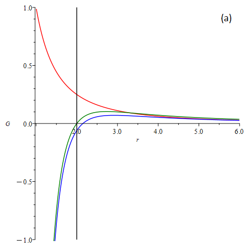
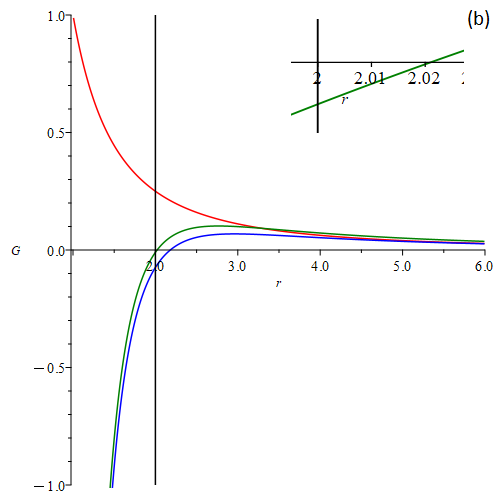
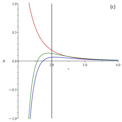
Figure 1: Plot (a) shows the function $G$ versus the distance $r$ for $N=-4.972,\,l=1.514,\,\alpha=0.5$ and $\mathcal{M}=1$. Plot(b) shows the function $G$ versus the distance $r$ for $N=-5.186,\,l=1.567,\alpha=0.5$ and $\mathcal{M}=1$, the small picture shows the function $G$ of hairy Kiselev black hole in the horizon vicinity. Plot (c) shows the function $H$ versus the distance $r$ for $N=-5.186,\,l=1.567,\alpha=0.5$ and $\mathcal{M}=1$. The red, blue, and green curves represent the Schwarzschild, Kiselev, and hairy Kiselev cases, respectively.

In order to understand better the influence of a primary hair on a geodesic motion we put $\alpha=0.1$ in order to consider bigger values of $l$. Figures 2(a) and 2(b) show how $G$ changes with different values of $l$ and $N$. One can see that there are regions where it becomes negative. However, from these pictures one cannot realize if they deal with a black hole or a naked singularity. For this purpose one should impose the condition of existence of an event horizon . The Figure 2(c) shows how $G$ changes in this case.

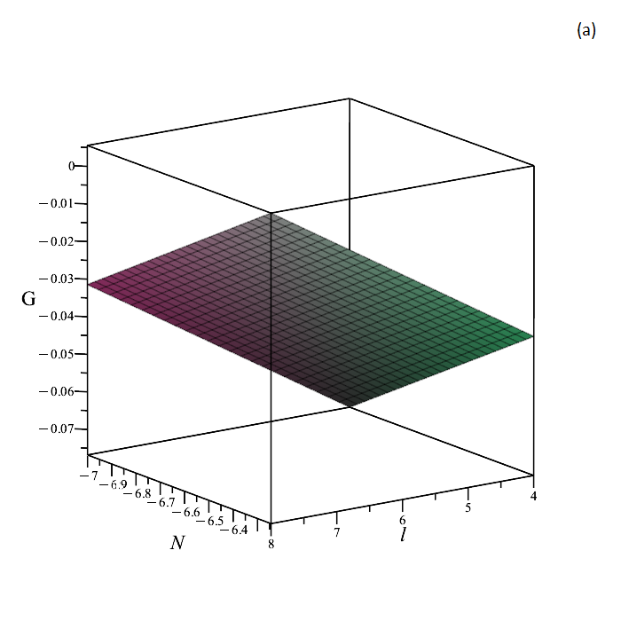
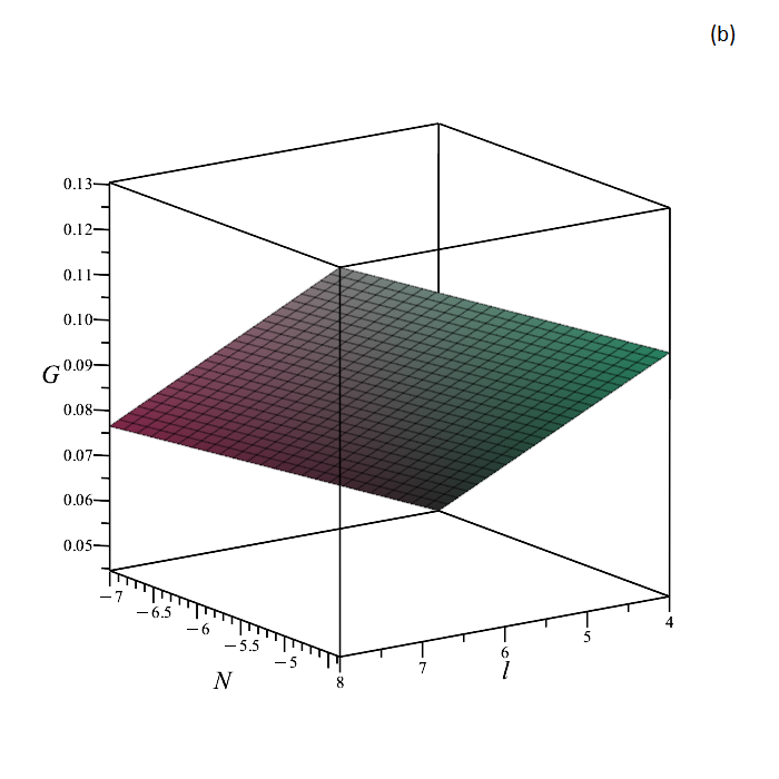
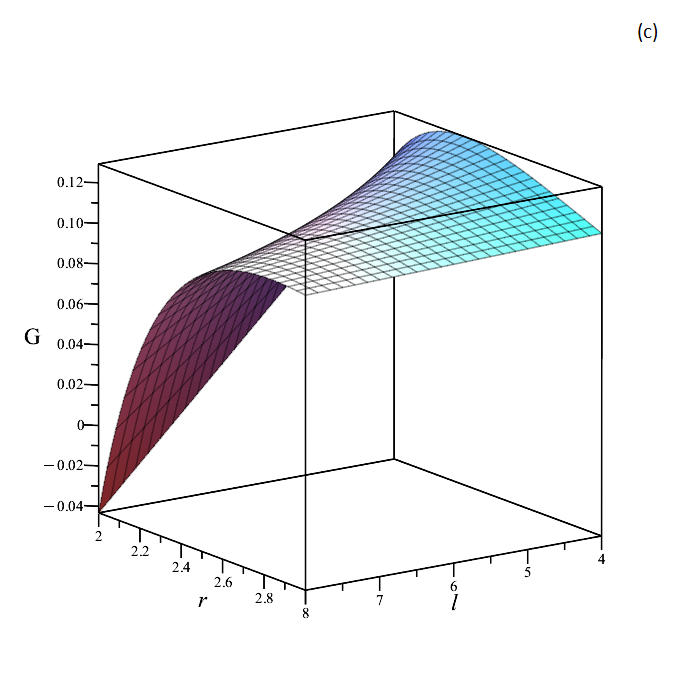
Figure 2: Plot(a) shows the function $G$ versus the parameters $N\in[-7,-6.245],\,l\in[4,8]$ for $r=2.1,\,\alpha=0.1$ and $\mathcal{M}=1$. Plot(b) shows the function $G$ versus the parameters $N\in[-7,-4.367],\,l\in[4,8]$ for $r=2.5,\,\alpha=0.1$ and $\mathcal{M}=1$. Plot(c) shows the function $G$ versus $l\in[4,8],\,r\in[2,3]$ for $N\in[-6.183,-2.983],\,\alpha=0.1$ and $\mathcal{M}=1$. The event horizon, located at $r=2\mathcal{M}$, follows the condition $N=-0.8l+1.6e^{-2}$.

4.2 Radiation

Here we consider the surrounding field having the average equation of state of radiation field as

$$P=\frac{\rho}{3}\,\Leftrightarrow\,\omega=\frac{1}{3}\,.$$ (51)

In this case, the $N$ parameter must be negative, and akin to the previous case, the surrounding radiation field and primary hairs weaken the forces in (48) and (49).

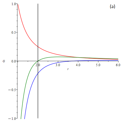
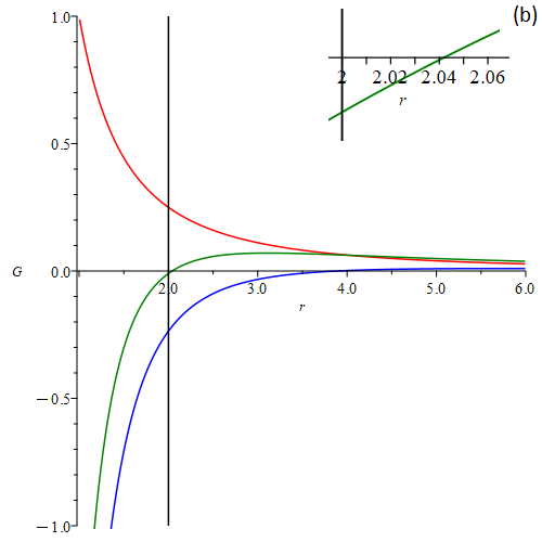
Figure 3: Plot(a) shows the function $G$ versus the distance $r$ for $N=-3.729,\,l=4,\,\alpha=0.5$ and $\mathcal{M}=1$. Plot(b) shows $G$ versus $r$ for $N=-3.889,\,l=4.16,\,\alpha=0.5$ and $\mathcal{M}=1$, the small picture shows the function $G$ of hairy Kiselev black hole in the horizon vicinity. Plot(c) shows $H$ versus $r$ for $N=-3.889,\,l=4.16,\,\alpha=0.5$ and $\mathcal{M}=1$. The red, blue, and green curves correspond to the Schwarzschild, Kiselev, and hairy Kiselev cases, respectively.

Figure 3(a) shows three curves in the pure Schwarzschild, Kiselev and hairy Kiselev black holes for the parameter values $N=-3.729$ and $l=4$. For the case of surrounding radiationlike field, one observes that the spacetime is akin to the hairy Reissner-Nordstrom black hole such that the parameter $N$ plays the role of black hole’s electric charge, i.e. $N=-Q^{2}$. So, in purely Reissner-Nordstrom case, the curve corresponds to the naked singularity because $\mathcal{M}^{2}<Q^{2}$. In comparison to the stiff fluid case, one notes that the parameters $l$ and $N$ are taken greater values to ensure that the function $G$ is negligible.

In Figure 3(b), we plotted curves in order to show that hairs can affect the geodesic motion and hence $G$ can become negative in the event horizon vicinity (in the region $2\leq r\leq 2.042$). In this case, we set $N=-3.889$ and $l=4.16$. One can see that the smaller values of $\omega$ we take, the bigger values of $l$ are required to ensure the negative values of $G$. For example, if we take this value of $l$ (i.e., $l=4.16$), then in the case of stiff fluid, we have $N=-15.557$ (we obtain this value by demanding that the event horizon is located at $r=\mathcal{M}$), then the $G$ function is negative in the region $2\leq r\leq 2.534$. Thus, one can see that the region, where negative values of $G$ are possible, shrinks when $\omega$ tends to zero. Figure 3(c) denotes the function $H$ with the values of $N$ and $l$ as in the previous figure.

Similar to the stiff fluid case, we have several plots for $\alpha=0.1$. Figures 4(a) and 4(b) show that $G$ becomes negative at the larger distances in comparison to the stiff fluid case. This apparently contradicts our previous statement that the smaller $\omega$ we consider, the region where $G$ becomes negative becomes smaller. However, one notes that this is a case of the naked singularity because if one imposes an extra condition of the event horizon existence, then for this case ($\alpha=0.1$) the $G$ function is always positive outside the horizon as can be seen from Figure 4(c).

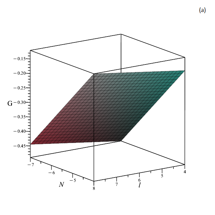
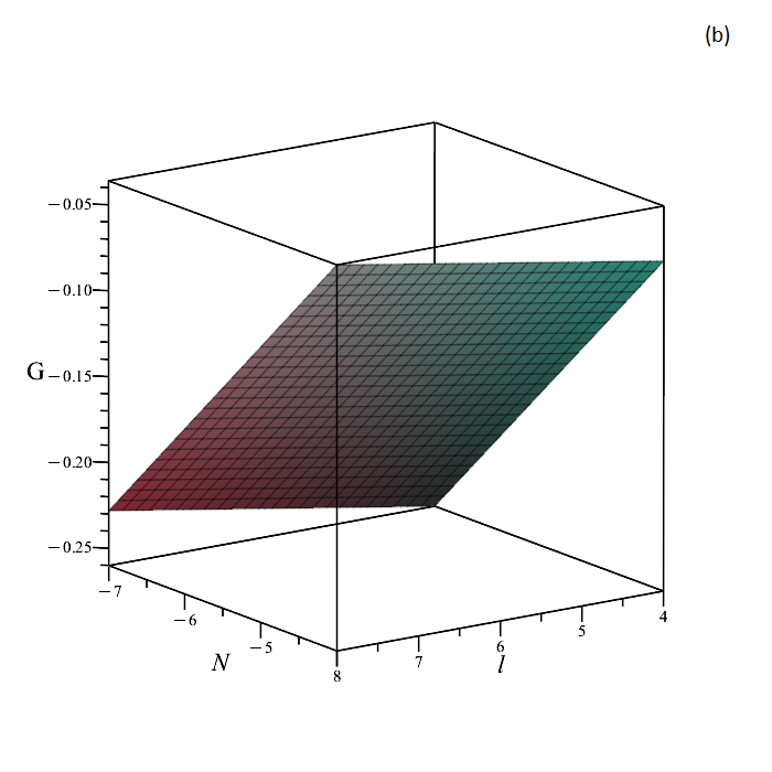
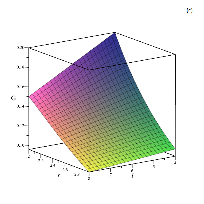
Figure 4: Plot(a) shows the function $G$ versus the parameters $N\in[-7,-4],\,l\in[4,8]$ for $r=2.1,\,\alpha=0.1$ and $\mathcal{M}=1$. Plot(b) shows the function $G$ versus the parameters $N\in[-7,-4],\,l\in[4,8]$ for $r=2.5,\,\alpha=0.1$ and $\mathcal{M}=1$. Plot(c) shows the function $G$ versus $r,\,l$ for $N\in[-1.546,-0.746],\,\alpha=0.1$ and $\mathcal{M}=1$. The event horizon, located at $r=2\mathcal{M}$, must satisfy the condition $N=-0.2l+0.4e^{-2}$.

4.3 Dust

For a dustlike field we have

$$P=0\,\Leftrightarrow\,\omega=0\,,$$ (52)

and we can show analytically that the function $G$ is positive near the event horizon as follows. We have

$$\frac{2M+N}{r}=1+\alpha e^{-\frac{r}{\mathcal{M}}}\,.$$ (53)

Substituting this into (48) and considering the event horizon at $r=2\mathcal{M}$, one obtains

$$\frac{1}{4\mathcal{M}}-\frac{\alpha}{4\mathcal{M}e^{2}}>0\,.$$ (54)

So, for physically relevant values of $\alpha,\,l$ and $N$, the function $G$ is positive outside the event horizon.

Figure 5(a) compares three curves of a hairy Kiselev black hole, purely Kiselev when $\alpha=0$, and Schwarzschild case when $\alpha=0$ and $N=0$. These curves are plotted for $l=0.5\,,N=-0.115$. Figure 5(b) is plotted for the same values of black hole parameters and shows the behaviour of the function $H$. For $\omega\geq 0$ the function $H$ is positive, and its behaviour is shown in the Figure 5(c). For other values of $\omega$ we could not find the condition (at small values of $\alpha$) where $H$ becomes negative.

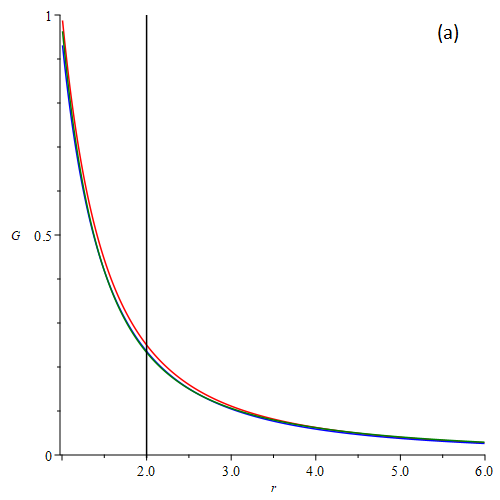
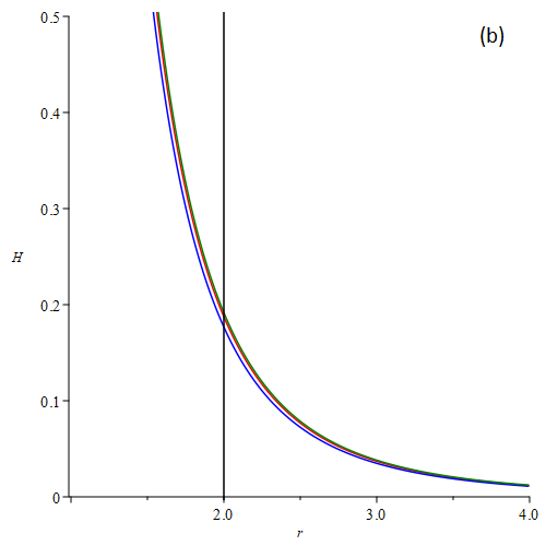
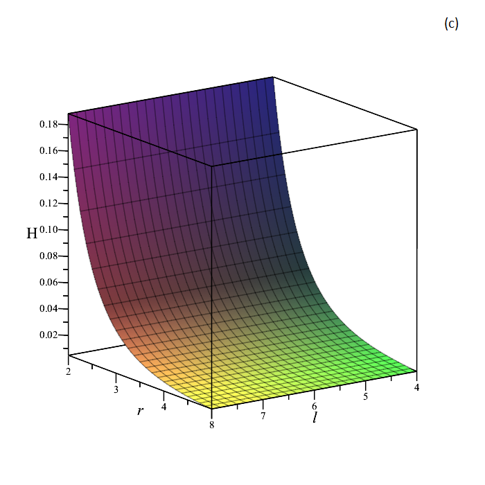
Figure 5: Plot(a) shows the function $G$ versus the distance $r$ for $N=-0.115,\,l=0.5,\alpha=0.5$ and $\mathcal{M}=1$. Plot(b) shows the function $H$ versus the distance $r$ for $N=-0.115,\,l=0.5,\,\alpha=0.5$ and $\mathcal{M}=1$. The red, blue, and green curves correspond to the Schwarzschild, Kiselev, and hairy Kiselev cases, respectively. Plot(c) shows the function $H$ versus $r\,,l$ for the values $N\in[-0.773,-0.373],\,l\in[4,8],\,r\in[2,5],\,\alpha=0.1$ and $\mathcal{M}=1$. The event horizon, located at $r=2\mathcal{M}$, must satisfy the condition $N=-0.1l+0.2e^{-2}$.

4.4 Quintessence

For a quintessencelike field, the equation of the state is

$$P=-\frac{2}{3}\rho\,\Leftrightarrow\,\omega=-\frac{2}{3}\,.$$ (55)

In this case, the parameter $N$ must be positive as one can see from (32). The function $G$ can be negligible in the vicinity of the horizon only if either $N$ or $L$ are negative. However, $G$ can take negative values but at large distances from the event horizon. As can be shown from Figure 6(a) at values $l=0.05\,,N=0.028$, the function $G$ for Kiselev black hole becomes negative at $r>8.553$. The effect of $N$ and $\alpha$ on the function $H$ for these values are negligible and they become considerable only at large distances, as one can see from Figure 6(b) .

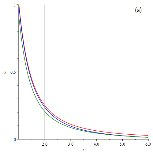
Figure 6: Plot(a) shows the function $G$ versus the distance $r$ for $N=0.028,\,l=0.05,\alpha=0.5$ and $\mathcal{M}=1$. Plot(b) shows the function $H$ versus the distance $r$ for $N=0.028,\,l=0.05,\,\alpha=0.5$ and $\mathcal{M}=1$. The red, blue, and green curves correspond to the Schwarzschild, Kiselev, and hairy Kiselev cases, respectively.

4.5 De Sitter background

In this case, the surrounded fluid has the effective equation of the state

$$P=-\rho\,\Leftrightarrow\,\omega=-1\,.$$ (56)

Like in the previous case, the parameter $N$ must be negative, and the function $G$ must be positive near the event horizon.

Figure 7(a) shows that the function $G$ for $N=0.016\,,l=0.01$ becomes negative for $r>3.841$. The function $H$ behaves very similar in all three cases as can be seen in Figure 7(b).

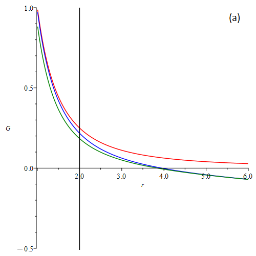
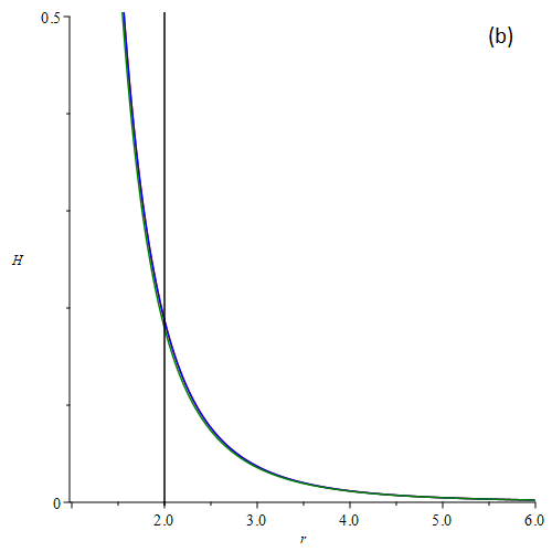
Figure 7: Plot(a) shows the function $G$ versus the distance $r$ for $N=0.016,\,l=0.01,\,\alpha=0.5$ and $\mathcal{M}=1$.Plot(b) shows the function $H$ versus the distance $r$ for the same values of parameters. The red, blue, and green curves correspond to the Schwarzschild, Kiselev, and hairy Kiselev cases, respectively.

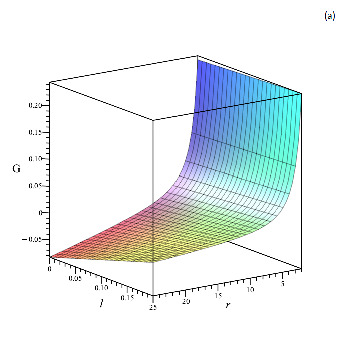
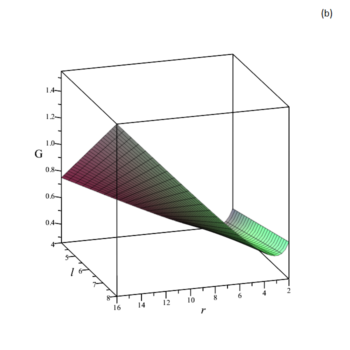
Figure 8: Plot (a): the dependence of the function $G$ on the $r\,,l$ for the values $N=0.003..0.0008\,,l=0..0.2\,,r=2..25\,,\alpha=0.1$ and $\mathcal{M}=1$. The event horizon, when it is located at $r=2\mathcal{M}$, must satisfy the following condition $N=-0.0125l+0.025e^{-2}$. Plot (b): the dependence of the function $G$ on the $r\,,l$ for the values $N=-0.047..-0.097\,,l=4..8\,,r=2..16\,,\alpha=0.1$ and $\mathcal{M}=1$. The event horizon, when it is located at $r=2\mathcal{M}$, must satisfy the following condition $N=-0.0125l+0.025e^{-2}$.

Figure 8 shows the behaviour of $G$ at $\alpha=0.1$ and with an extra condition of the event horizon existence. Here 8(a) is plotted for positive cosmological constant as 8(b) for negative cosmological constant - anti-de-Sitter case.

4.6 Phantom field

In general, the equation of the state a phantomlike field lies in the range $\omega<-1$ [75, 76, 77, 78, 79, 80, 81]. In order to study the effect of a phantom field, one can consider, as instance

$$P=-\frac{4}{3}\rho\,\Leftrightarrow\,\omega=-\frac{4}{3}\,.$$ (57)

The parameter $N$ must be positive, and as can be seen in Figure 9(a), the function $G$ takes negative values at the region $r>3.056$ at $l=0.05\,,N=0.007$. Figure 9(b) shows that for the same values of $l$ and $N$, the function $H$ can be negative in the region $r>5.433$.

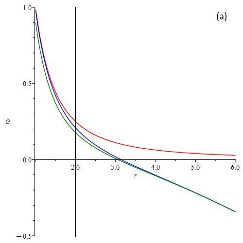
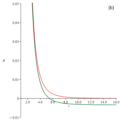
Figure 9: Plot(a) shows the function $G$ versus the distance $r$ for $N=0.007\,,l=0.05,\alpha=0.5$ and $\mathcal{M}=1$. Plot(b) shows the function $H$ versus the distance $r$ for $N=0.007\,,l=0.05,\alpha=0.5$ and $\mathcal{M}=1$. The red, blue, and green curves correspond to the Schwarzschild, Kiselev, and hairy Kiselev cases, respectively.

5 Conclusion

Inspired by the fact that black holes inhabit nonvacuum cosmological backgrounds, we present a new solution to the Einstein field equations representing a surrounded hairy Schwarzschild black hole. This solution takes into account both the primary hair and surrounding fields (represented by an energy-momentum tensor following the linearity and additivity condition [21]), which affect the properties of the black hole. The effect of the corresponding contributions on timelike geodesics are discussed. We find that the new induced modifications can be considerable in certain cases. In particular, we investigate how the specified surrounding fields and primary hairs affect the Newtonian and perihelion precession terms. Our observations are as follows.

• The surrounding fields with $-\frac{1}{3}<\omega<0$ contribute positively to the Newtonian term, i.e ., strengthening the gravitational attraction.

• The new corrections to the Newtonian term might be the same order or even greater for all other cases if one considers a naked singularity .

• In the case that the solution represents a black holes, new corrections can be of the same order or even greater than the Newtonian term in the event horizon vicinity for $\omega>0$.

• For $\omega<-\frac{1}{3}$, i.e., for effectively repulsive fluids akin to dark energy models, the correction terms dominate far from the event horizon and mainly near the cosmological horizon.

The Schwarzschild black hole is an idealized vacuum solution, and it is important to consider how it gets deformed in the presence of matter fields. Another crucial factor to consider is the impact of the surrounding environment, particularly the shadow of a black hole in the cosmological background, which serves as a potential cosmological ruler [58]. The solution presented in this work can be further investigated to study the shadow of a hairy Schwarzschild black hole in various cosmological backgrounds in order to find out how anisotropic fluid can affect the observational properties [74], which is a plan of our upcoming investigations. It is worthwhile to mention that applying the Newman-Janis [59] and Azreg Ainou [60, 61] algorithms one can obtain the rotating version of the solution presented here. Also, investigation of quasinormal modes, thermodynamics properties, accretion process, and gravitational lensing of these solutions can help us to understand better the nature of these objects.

The obtained hairy Kiselev solution has many potential uses in various cosmological and astrophysical scenarios. It can be an arena for high-energy phenomena. If one considers the centre of mass energy $E_{c.m.}$ of two colliding particles in usual Schwarzschild spacetime, than the value is quite limited and small [14]. However, two extra terms here might lead to the existence of the innermost stable equilibrium point in the horizon vicinity [15], which can lead to unbound centre-of-mass energy $E_{c.m.}$ of two colliding particles. Another tool to distinguish the hairy Kiselev black hole from the usual Schwarzschild one is to study its shadow properties. The shape of the shadow is the same as in the Schwarzschild case due to the spherical symmetry. However, the existence of four extra parameters $\omega\,,N\,,\alpha\,,l$ have, surely, impact on its size and intensity [62]. The study of the planet’s motion is the way to define if a primary hair can have an impact on its trajectory . As we have shown, extra terms can drastically change particle motion. However, in a realistic astrophysical situation, one should consider this motion near the black hole where $\alpha\,,l\,,N$ has a large impact on the particle motion. Based on the parameters and variables considered in this model, it seems that attempting to test it within the Solar system would be futile. This is because any additional terms are essentially insignificant beyond the surface of the Sun, resulting in a prediction that would be indistinguishable from that which is already predicted in Schwarzschild spacetime. Therefore, it may be more beneficial to focus on the study of black hole vicinity where more noticeable results can be achieved. Although it has not yet been observed, the Hawking temperature and radiation may get also influenced by a primary hair [55, 56]. The Schwarzschild black hole possesses a negative heat capacity. Cosmological fields and primary hair might lead to positive specific heat capacity and phase transition [63]. All these are the topics of our future investigations.

Acknowledgments: V. Vertogradov and M. Misyura say thanks to grant NUM. 22-22-00112 RSF for financial support.

References

- [1] The Event Horizon Telescope Collaboration, First M87 Event Horizon Telescope results. I. The shadow of the supermassive black hole, Astrophys. J. Lett. 875 (2019) L1
- [2] The Event Horizon Telescope Collaboration, First M87 Event Horizon Telescope results. II. Array and instrumentation, Astrophys. J. Lett. 875 (2019) L2
- [3] The Event Horizon Telescope Collaboration, First M87 Event Horizon Telescope results. III. Data processing and calibration, Astrophys. J. Lett. 875 (2019) L3
- [4] Akiyama, K. et al. [Event Horizon Telescope Collaboration]. First Sagittarius A* Event Horizon Telescope Results. I. The Shadow of the Supermassive Black Hole in the Center of the Milky Way. Astrophys. J. Lett. 2022, 930, L12.
- [5] R. Penrose and R. M. Floyd, Extraction of Rotational Energy from a Black Hole Nature Physical Science 229, 177 (1971).
- [6] O. B. Zaslavskii, Energy extraction from extremal charged black holes due to the Banados-Silk-West effect Phys. Rev. D 86, 124039 (2012) [arXiv:1207.5209]
- [7] Lucas Timotheo Sanches, Mauricio Richartz. Energy extraction from non-coalescing black hole binaries Phys. Rev. D 104, 124025(2021), arXiv:2108.12408 (gr-qc)
- [8] Vitalii Vertogradov, Extraction energy from charged Vaidya black hole via the Penrose process 2023 Commun. Theor. Phys. 75 045404
- [9] O. B. Zaslavskii, Negative energy states in the Reissner-Nordstrom metric Mod. Phys. Lett. A 36, 2150120 (2021), arXiv:2006.02189 [gr-qc].
- [10] Grib A.A., Pavlov Yu.V., Vertogradov V.D. Geodesics with negative energy in the ergosphere of rotating black holes. Modern Physics Letters A. Vol. 29,Iss. 20. 2014- P. 14501-14510. [arXiv:1304.7360]
- [11] V. Vertogradov, The Negative Energy in Generalized Vaidya Spacetime Universe 6(9), 155 (2020), arXiv:2209.10976 [gr-qc]
- [12] Vertogradov V.D. Geodesics with negative energy in the ergosphere of rotating black holes, Gravitation and Cosmology. Vol. 21, Iss. 2. 2015.- PP. 171-174. [arXiv:2210.04674]
- [13] E. Babichev, V. Dokuchaev, Yu. Eroshenko, Black Hole Mass Decreasing due to Phantom Energy Accretion Phys. Rev. Lett. 93, 021102 (2004).
- [14] M. Banados, J. Silk, S.M. West, Kerr Black Holes as Particle Accelerators to Arbitrarily High Energy Phys. Rev. Lett. 103, 111102 (2009) [arXiv:0909.0169].
- [15] O. B. Zaslavskii, Acceleration of particles by black holes as a result of deceleration: Ultimate manifestation of kinematic nature of BSW effect Phys. Lett. B 712 (2012) 161 [arXiv:1202.0565]
- [16] O. B. Zaslavskii, Circular orbits and acceleration of particles by near-extremal dirty rotating black holes: general approach. Class. Quantum Grav. 29 (2012) 205004 [arXiv:1201.5351 [gr-qc]]
- [17] Grib, A. A., Pavlov Y. V. (2020) Rotating black holes as sources of high energy particles. Physics of Complex Systems, 1 (1), 40-49.DOI: 10.33910/2687-153X-2020-1-1-40-49
- [18] Vertogradov, V.D. (2023) On particle collisions during gravitational collapse of Vaidya spacetimes. Physics of Complex Systems, 4 (1), 17-23.
- [19] Mandar Patil, Tomohiro Harada, Ken-ichi Nakao, Pankaj S. Joshi, Masashi Kimura, Infinite efficiency of collisional Penrose process: Can over-spinning Kerr geometry be the source of ultra-high-energy cosmic rays and neutrinos? Phys. Rev. D 93, 104015 (2016) [arXiv:1510.08205 [gr-qc]]
- [20] T. Harada, H. Nemoto, U. Miyamoto, Upper limits of particle emission from high-energy collision and reaction near a maximally rotating Kerr black hole Phys.Rev .D86:024027,2012 [arXiv:1205.7088]
- [21] V. V. Kiselev, Class. Quintessence and black holes Quant. Grav. 20, 1187 (2003).
- [22] Heydarzade, Y., Darabi, F. Surrounded Vaidya solution by cosmological fields. Eur. Phys. J. C 2018, 78, 582.
- [23] Heydarzade, Y.; Darabi, F. Surrounded Bonnor-Vaidya solution by cosmological fields. Eur. Phys. J. C 2018, 78, 1004.
- [24] Y. Heydarzade, F. Darabi Surrounded Vaidya black holes: apparent horizon properties, Eur. Phys. J. C (2018) 78:342.
- [25] R. Geroch and J.B. Hartle, Distorted black holes J. Math. Phys. 23, 680 (1982).
- [26] S. Fairhurst, B. Krishnan, Distorted Black Holes with Charge Int. J. Mod. Phys. D10, 691 (2001).
- [27] S.R. Brandt, E. Seidel, Evolution of distorted rotating black holes. III. Initial data Phys. Rev. D54, 1403 (1996).
- [28] M. Ansorg, D. Petroff, Black holes surrounded by uniformly rotating rings Phys. Rev. D 72.2, 024019 (2005).
- [29] S. W. Hawking, Black holes in general relativity Commun. Math. Phys. 25, 152 (1972).
- [30] J.D. Brown and V. Husian, Black holes with short hair Int. J. Mod. Phys. D6, 563 (1997).
- [31] S.Droz, M. Heusler, N. Straumann, New black hole solutions with hair Phys. Lett. B, 268 (3-4), 371 (1991).
- [32] J. Barranco, A. Bernal, J.C. Degollado, A. Diez-Tejedor, M. Megevand, M. Alcubierre, D. Ndnez, O. Sarbach, Schwarzschild Black Holes can Wear Scalar Wigs Phys. Rev. Lett. 109, 081102 (2012).
- [33] J.D. Bekenstein, Novel ”no-scalar-hair” theorem for black holes Phys. Rev. D 51(12), R6608 (1995).
- [34] Hawking, S.W.; Perry, M.J.; Strominger, A. Soft Hair on Black Holes. Phys. Rev. Lett. 2016, 116, 231301.
- [35] J. Ovalle, Extending the geometric deformation: New black hole solutions. Int. J. Mod. Phys. Conf. Ser., 41, 1660132 (2016) [arXiv:1510.00855 [gr-qc]]
- [36] Roberto Casadio, Jorge Ovalle, Roldao da Rocha, The Minimal Geometric Deformation Approach Extended. Class. Quantum Grav. 32 (2015) 215020 [arXiv:1503.02873 [gr-qc]]
- [37] Ovalle, J.; Casadio, R.; Rocha, R.D.; Sotomayor, A.; Stuchlik, Z. Black holes by gravitational decoupling. Eur. Phys. J. C 2018, 78, 960.
- [38] Ovalle, J. Decoupling gravitational sources in general relativity: From perfect to anisotropic fluids. Phys. Rev. 2017, D95, 104019.
- [39] Ovalle, J. Decoupling gravitational sources in general relativity: The extended case. Phys. Lett. B 2019, 788, 213.
- [40] Contreras, E.; Ovalle, J.; Casadio, R. Gravitational decoupling for axially symmetric systems and rotating black holes. Phys. Rev. D 2021, 103, 044020.
- [41] Ovalle, J.; Casadio, R.; Contreras, E.; Sotomayor, A. Hairy black holes by gravitational decoupling. Phys. Dark Universe 2021, 31, 100744.
- [42] S. Mahapatra and I. Banerjee, Rotating hairy black holes and thermodynamics from gravitational decoupling, Phys. Dark Univ. 39 (2023) 101172 [arXiv: 2208.05796],
- [43] Vitalii Vertogradov, Maxim Misyura ”Vaidya and Generalized Vaidya Solutions by Gravitational Decoupling”Universe 2022, 8(11), 567; doi:10.3390/universe8110567 [arXiv:2209.07441 [gr-qc]]
- [44] Vitalii Vertogradov, Maxim Misyura, The Regular Black Hole by Gravitational Decoupling. Phys. Sci. Forum 2023, 7(1), 27
- [45] Jorge Ovalle, Roberto Casadio, Andrea Giusti, Regular hairy black holes through Minkowski deformation. [arXiv:2304.03263 [gr-qc]]
- [46] M. Jamil, S. Hussain, Dynamics of particles around a Schwarzschild-like black hole in the presence of quintessence and magnetic field B. Majeed, Eur. Phys. J. C 75. 1, 24 (2015).
- [47] I. Hussain, S. Ali, Marginally stable circular orbits in the Schwarzschild black hole surrounded by quintessence matter Eur. Phys. J.l Plus 131. 8, 275 (2016).
- [48] B. Malakolkalami, K. Ghaderi, The null geodesics of the Reissner-Nordstrom black hole surrounded by quintessence Mod. Phys. Lett . A 30 .10, 1550049 (2015).
- [49] S. Fernando, Schwarzschild black hole surrounded by quintessence: Null geodesics Gen. Rel. Grav. 44.7, 1857 (2012).
- [50] R. Uniyal, N.C. Devi, Geodesic Motion in Schwarzschild Spacetime Surrounded by Quintessence H. Nandan, K.D. Purohit, Gen. Rel. Grav. 47.2, 16 (2015).
- [51] S. Fernando, S. Meadows, K. Reis, Null Trajectories and Bending of Light in Charged Black Holes with Quintessence Int. J. Theo. Phys. 54.10, 3634 (2015).
- [52] Ramos, A.; Arias, C.; Avalos, R.; Contreras,E. Geodesic motion around hairy black holes. Annals Phys. 2021, 431, 168557.
- [53] Sohan Kumar Jha, Anisur Rahaman, Gravitational lensing by the hairy Schwarzschild black hole. arXiv:2205.06052[gr-qc]
- [54] Zhen Li, Faqiang Yuan, Energy extraction via Comisso-Asenjo mechanism from rotating hairy black hole. [arXiv:2304 .12553 [gr-qc]]
- [55] Cavalcanti, R.T.; Alves, K.d.S.; da Silva, J.M.H. Near horizon thermodynamics of hairy black holes from gravitational decoupling. Universe 2022, 8, 363.
- [56] Vertogradov V. D., Kudryavcev D. A. On the temperature of hairy black holes. Physics of Complex Systems. Vol. 4, no. 2, 2023
- [57] Y. Heydarzade, F. Darabi, Black Hole Solutions Surrounded by Perfect Fluid in Rastall Theory Phys. Lett. B, 771, 365 (2017).
- [58] Oleg Yu. Tsupko, Zuhui Fan, Gennady S. Bisnovatyi-Kogan, Black hole shadow as a standard ruler in cosmology. Classical and Quantum Gravity, 37, 065016 (2020) [arXiv:1905.10509 [gr-qc]]
- [59] E. T. Newman and A. I. Janis, ”Note on the Kerr spinning particle metric,” 10.1063/1 J. Math. Phys. 6 (1965) 915-917.
- [60] M. Azreg-Ainou, ”Regular and conformal regular cores for static and rotating solutions,” 10.1016/j.physletb.2014.01 Phys. Lett. B 730 (2014) 95-98, [arXiv:1401.0787 [gr-qc]].
- [61] M. Azreg-Ai’nou, ”From static to rotating to conformal static solutions: Rotating imperfect fluid wormholes with(out) electric or magnetic field,” epjc/s10052-014-2865-8 Eur. Phys. J. C 74 no. 5, (2014) 2865, [arXiv:1401.4292 [gr-qc]].
- [62] Rajibul Shaikh and others, Shadows of spherically symmetric black holes and naked singularities, Monthly Notices of the Royal Astronomical Society, Volume 482, Issue 1, January 2019, Pages 52-64
- [63] Saleh, M., Thomas, B.B. Kofane, T.C. Thermodynamics and Phase Transition from Regular Bardeen Black Hole Surrounded by Quintessence. Int J Theor Phys 57, 2640-2647 (2018). https://doi.org/10 .1007/s10773-018-3784-5
- [64] Ovalle, J., Contreras, E. Stuchlik, Z. Energy exchange between relativistic fluids: the polytropic case. Eur. Phys. J. C 82, 211 (2022). https://doi.org/10.1140/epjc/s10052-022-10168-5
- [65] Gabbanelli, L., Rincón, Á. Rubio, C. Gravitational decoupled anisotropies in compact stars. Eur. Phys. J. C 78, 370 (2018). https://doi.org/10.1140/epjc/s10052-018-5865-2
- [66] C. Deffayet, S. Deser, and G. Esposito-Farèse, Arbitrary -form Galileons Phys. Rev. D 82, 061501 (R)
- [67] Ángel Rincón and Grigoris Panotopoulos , Quasinormal modes of scale dependent black holes in -dimensional Einstein-power-Maxwell theory Phys. Rev. D 97, 024027
- [68] Rincón, Á., Contreras, E., Bargueño, P. et al. Scale-dependent three-dimensional charged black holes in linear and non-linear electrodynamics. Eur. Phys. J. C 77, 494 (2017). https://doi.org/10 .1140/epjc/s10052-017-5045-9
- [69] Benjamin Koch et al, A scale dependent black hole in three-dimensional space-time, 2016 Class. Quantum Grav. 33 225010
- [70] Rebecca Briffa et al, Constraining teleparallel gravity through Gaussian processes, 2020 Class. Quantum Grav. 38 055007
- [71] Grigoris Panotopoulos, Ángel Rincón, and Ilídio Lopes, Orbits of light rays in scale-dependent gravity: Exact analytical solutions to the null geodesic equations Phys. Rev. D 103, 104040
- [72] Grigoris Panotopoulos, Ángel Rincón, Orbits of light rays in -dimensional Einstein-power-Maxwell gravity: Exact analytical solution to the null geodesic equations, Annals of Physics, Volume 443, 2022, 168947 https://doi.org/10.1016/j.aop.2022.168947
- [73] Avalos, R., Bargueño, P., Contreras, E., A Static and Spherically Symmetric Hairy Black Hole in the Framework of the Gravitational Decoupling. Fortschr. Phys. 2023, 71, 2200171. https://doi.org/10.1002/prop.202200171
- [74] Sunny Vagnozzi et al, Horizon-scale tests of gravity theories and fundamental physics from the Event Horizon Telescope image of Sagittarius A, 2023 Class. Quantum Grav. 40–165007
- [75] Parampreet Singh, M. Sami, and Naresh Dadhich, Cosmological dynamics of a phantom field, Phys. Rev. D 68, 023522
- [76] Dzhunushaliev V., Folomeev V., Myrzakulov K., Myrzakulov R., Phantom fields: bounce solutions in the early Universe and s-branes, International Journal of Modern Physics DVol. 17, No. 12, pp. 2351–2358 (2008)
- [77] Chakraborty, S., Debnath, U. The Effects of Tachyonic and Phantom Fields in the Intermediate and Logamediate Scenarios of the Anisotropic Universe. Int J Theor Phys 51, 1224-1238 (2012). https://doi.org/10.1007/s10773-011-0998-1.
- [78] G.W. Gibbons, Phantom Matter and the Cosmological Constant, arXiv:hep-th/0302199.
- [79] I. Maor, R. Brustein, J. McMahon, and P.J. Steinhardt, Measuring the equation of state of the universe: Pitfalls and prospects, Phys. Rev. D 65, 123003 (2002).
- [80] A. E. Schulz, M. White, The Tensor to Scalar Ratio of Phantom Dark Energy Models, Phys. Rev. D 64, 043514 (2001).
- [81] R.R. Caldwell, A Phantom Menace. Cosmological consequences of a dark energy component with super-negative equation of state, Phys. Lett. B 545, 23 (2002).