SuppMaterial

Beyond the Two-Trials Rule

1 Introduction

The two trials rule is a standard requirement by the FDA to demonstrate efficacy of drugs. It demands “at least two pivotal studies, each convincing on its own” [1] before drug approval is granted and “reflects the need for substantiation of experimental results, which has often been referred to as the need for replication of the finding” [2]. The rule is usually implemented by requiring two independent studies to be significant at the standard (one-sided) $\alpha=0.025$ level [3, Sec. 12.2.8]. Statistical justification for the two-trials rule is usually based on a hypothesis testing perspective where Type-I error (T1E) control is the primary goal. The T1E rate is the probability of a false claim of success under a certain null hypothesis. Two different null hypotheses are relevant if results from two studies are available: The intersection null hypothesis

$$H^{\,1}_{0}\cap H^{\,2}_{0}$$ (1)

is a point null hypothesis, defined as the intersection of the study-specific null hypotheses $H^{\,i}_{0}$: $\theta_{i}=0$, $i=1,2$, here $\theta_{i}$ denotes the true effect size in the $i$-th study. The probability of a false claim of success with respect to the intersection null (1) is the overall or project-wise T1E rate [4]. The overall T1E rate of the two-trials rule is $\alpha^{2}=0.025^{2}=0.000625$, because the two studies are assumed to be independent.

The no-replicability or union null hypothesis is defined as the complement of the alternative hypothesis that the effect is non-null in both studies [5, 6, 7]. This is a composite null hypothesis, which also includes the possibility that only one of the studies has a null effect:

$$H^{\,1}_{0}\cup H^{\,2}_{0}.$$ (2)

I follow Micheloud et al. [8] and call the probability of a false claim of success with respect to the union null (2) the partial T1E rate. The partial T1E rate depends on the values of $\theta_{1}$ and $\theta_{2}$, where one of the two parameters must be zero but the other one may not be zero. The partial T1E rate of the two-trials rule is bounded from above by $\alpha$, the exact value depends on the difference $\theta_{1}-\theta_{2}$ [9].

The FDA has recently emphasized that “two positive trials with differences in design and conduct may be more persuasive, as unrecognized design flaws or biases in study conduct will be less likely to impact the outcomes of both trials” [2]. The FDA also notes that two trials with distinct study populations or different clinical endpoints provide more evidence of benefit than two positive identically designed and conducted trials, which “could leave the conclusions of both trials vulnerable to any systematic biases inherent to the particular study design.” But only in the latter case the two trials can be considered as fully exchangeable where pooling the study results with a fixed-effect meta-analysis is a useful alternative [3, Sec. 12.2.8]. However, pooling does not control the partial T1E rate as one persuasive study may easily overrule the results from a second unconvincing study. This underlines the importance to control not only the overall but also the partial T1E rate. Of course, all trials considered should be “adequate and well-controlled”, otherwise we may just be interested in the effect estimates from the high quality studies [10].

In what follows I describe methods that aim to control both the overall T1E and partial T1E rates based on results from two (or three) adequately designed trials. In principle there are two options to develop alternatives to the two-trials rule, see Figure 1 for an illustration with Edgington’s method, described in Section 2.3 in more detail. First, we may consider methods with partial T1E rate bound at $\alpha$, but this will inevitably reduce the overall T1E rate and the project power, because the success region of any such method (in terms of the trial-specific $p$-values $p_{1}$ and $p_{2}$) must be a subset of the success region of the two-trials rule. Alternatively we may fix the overall T1E rate at $\alpha^{2}$ and allow for some inflation of the partial T1E rate. Now the success regions is no longer a subset of the success region of the two-trials rule, so the impact on project power is not immediate. The latter approach has been also selected by Rosenkranz [4] as an “overarching principle” in the search for generalizations of the two-trials rule. Our goal is thus to allow for some (limited) inflation of the partial T1E rate while maintaining overall T1E control.

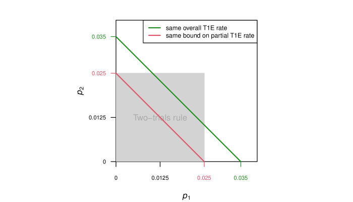
Figure 1: Illustration of partial and overall T1E control with Edgington’s method. The grey squared region represents the success region of the two-trials rule in terms of the two (one-sided) $p$-values $p_{1},p_{2}\leq\alpha=0.025$, so the partial T1E rate is controlled at $\alpha$ and the overall T1E rate is $\alpha^{2}$. The success region below the red line also controls the partial T1E rate at $\alpha$, but has reduced overall T1E rate of $\alpha^{2}/2$. The success region below the green line controls the partial T1E rate at $\sqrt{2}\,\alpha\approx 0.035$ and has overall T1E rate $\alpha^{2}$, the same as for the two-trials rule.

Instead of the “double dichotomization” of the two-trials rule I propose to base inference on $p$-value combination methods which return a combined $p$-value that can be interpreted as a quantitative measure of the total available evidence. However, many standard combination methods do control the partial T1E rate only at the trivial bound 1, for example Fisher’s or Tippett’s method [5, 11]. Also Stouffer’s “inverse normal” method [12], which is closely related to a fixed effect meta-analysis and called the “pooled-trials rule” in Senn [13], does not control the partial T1E rate at a non-trivial bound. Indeed, all these methods can flag success even if one of the two studies is completely unconvincing with an effect estimate perhaps even significant in the wrong direction. This may be acceptable within a study to be able to stop an experiment at interim for efficacy [14], but is unacceptable to assess replicability across studies [15]. I therefore concentrate on less-known $p$-value combination methods that have an in-built non-trivial control of the partial T1E rate: The $n$-trials rule (requiring each of $n$ trials to be significant at a common significance level), Pearson’s and Edgington’s method, the harmonic mean $\chi^{2}$-test and the sceptical $p$-value.

The conclusion of this paper is a tentative recommendation for Edgington’s $p$-value combination method [16] as summarized in Box 1: Declare success if the sum of the (one-sided) $p$-values from the two studies is smaller than $\sqrt{2}\,\alpha\approx 0.035$. A single $p$-value can thus be larger than 0.025 to lead to success (but not larger than 0.035) as long the other one is sufficiently small. If three studies are considered, then the sum of the three $p$-values needs to be smaller than $\sqrt[3]{6\,\alpha^{2}}\approx 0.16$. A sequential version is also described in Box 1, where stopping for success after two studies is possible, otherwise a third study will be required. All these approaches control the overall T1E rate at $\alpha^{2}=0.025^{2}$ while ensuring that each study considered is “convincing on its own” to a sufficient degree, i. e. Edgington’s method has a non-trivial and sufficiently small bound on the partial T1E rate. Furthermore, the different versions have larger power to detect existing effects than the two- and three-trials rule, respectively, and other attractive properties.

Section 2 describes $p$-value combination methods with a non-trivial bound on the partial T1E rate. Section 3 compares these methods for data from two and three trials, respectively. For three trials we also discuss the 2-of-3 method recently proposed by Rosenkranz [4]. Section 4 develops sequential versions of some of the methods, which allow to stop early for success after two trials. A comparison in terms of project power and expected number of studies required is presented. I close with some discussion in Section 5.

2 P-value combination methods with partial T1E control

In the following I will describe $p$-value combination methods that control the partial T1E at a non-trivial bound different from 1. Throughout I will work with one-sided $p$-values $p_{1},\ldots,p_{n}$ and assume that the $p_{i}$’s are independent and uniformly distributed under the null hypothesis $H^{\,i}_{0}$: $\theta_{i}=0$, $i=1,\ldots,n$. Overall and partial T1E rate are now defined accordingly across all $n$ trials. Throughout I aim to achieve an overall T1E rate rate of $\alpha_{\cap}$, usually $\alpha_{\cap}=0.025^{2}=0.000625$.

2.1 The n-trials rule

The two-trials rule can easily be generalized to $n$ trials, where it is also known as Wilkinson’s method [17]. For example, $n=3$ independent trials need to achieve significance at level $\alpha_{\star}=\alpha^{2/3}$ to control the overall T1E rate at level $\alpha_{\cap}=\alpha_{\star}^{3}=\alpha^{2}$. For $\alpha=0.025$ we obtain $\alpha_{\star}=0.085$, so the partial T1E rate bound of the three-trials rule at overall level $\alpha_{\cap}=0.025^{2}$ is $0.085$. The general threshold is $\alpha_{\star}=\alpha^{2/n}$, which serves as a benchmark for other methods based on $n$ trials with overall T1E rate $\alpha_{\cap}=\alpha^{2}$. The combined $p$-value of the $n$-trials rule is $p=\max\{p_{1},p_{2},\ldots,p_{n}\}^{n}.$

2.2 Pearson’s combination test

Pearson’s combination method [18, 19] is a less-known variation of Fisher’s method. Fisher’s method [20] is based on the test statistic

$$F_{n}=-2\sum_{i=1}^{n}\log(p_{i})$$ (3)

which follows a $\chi^{2}_{2n}$ distribution if the $p$-values $p_{1},\ldots,p_{n}$ are independent uniformly distributed. Large values of $F_{n}$ provide evidence against the intersection null, and thresholding $F_{n}$ at the $(1-\alpha_{\cap})$-quantile $\chi^{2}_{2n}(1-\alpha_{\cap})$ of the $\chi^{2}_{2n}$-distribution gives the success criterion

$$\prod_{i=1}^{n}p_{i}\leq\exp\left\{-0.5\chi^{2}_{2n}(1-\alpha_{\cap})\right\}.$$ (4)

It follows that a sufficient (but not necessary) criterion for success is that at least one $p$-value fulfills

$$p_{i} \leq \exp\left\{-0.5\chi^{2}_{2n}(1-\alpha_{\cap})\right\}.$$ (5)

For example, for $n=2$ and $\alpha_{\cap}=0.025^{2}=0.000625$, the right-hand side of (5) is $0.00006$. If the first $p$-value $p_{1}$ is smaller than this bound, Fisher’s criterion (4) will flag success no matter what the result from the second study is and does therefore not control the partial T1E rate at a non-trivial bound.

Pearson’s method [18, 19] uses the fact that if $p_{i}$ is uniform also $1-p_{i}$ is uniform, so

$$K_{n}=-2\sum_{i=1}^{n}\log(1-p_{i})$$ (6)

also follows a $\chi^{2}_{2n}$ distribution under the intersection null. Now small values of $K_{n}$ provide evidence against the intersection null and we need to threshold $K_{n}$ at the $\alpha_{\cap}$-quantile $a_{n}=\chi^{2}_{2n}(\alpha_{\cap})$. This gives the success criterion $K_{n}\leq a_{n}$, or equivalently

$$\prod_{i=1}^{n}(1-p_{i})\geq\exp(-0.5\,a_{n}),$$ (7)

with corresponding combined $p$-value $p=\Pr(\chi^{2}_{2n}\leq K_{n})$. It follows from (7) that a necessary (but not sufficient) success criterion is that all $p$-values fulfill

$$p_{i} \leq 1-\exp(-0.5\,a_{n}).$$ (8)

For $n=2$ and $\alpha_{\cap}=0.025^{2}$ the right-hand side of (8) is $0.035$, which is then also the bound of Pearson’s method on the partial T1E rate and only slightly larger than for the two-trials rule where both $p$-values have to be smaller than 0.025.

2.3 Edgington’s method

Edgington [16] proposed a method that combines $p$-values by addition rather than multiplication as in Fisher’s criterion (4). Under the intersection null hypothesis, the distribution of the sum of the $p$-values

$$E_{n}=p_{1}+\ldots+p_{n}$$ (9)

follows the Irwin-Hall distribution [21, 22], denoted as $E_{n}\sim\operatorname{IH}(n)$, see also Johnson et al. [23, Section 26.9]. A combined $p$-value $p=\Pr(\operatorname{IH}(n)\leq E_{n})$ can be calculated using the cdf of the Irwin-Hall distribution, which is available in closed form. For $E_{n}\leq 1$, the computation is particularly simple:

$$p=(E_{n})^{n}/n!,$$ (10)

otherwise a correction term must be added [16].

Critical values $b_{n}$, which define success if and only if $E_{n}\leq b_{n}$, can be calculated by replacing $p$ with $\alpha_{\cap}=\alpha^{2}=0.025^{2}$ in (10) and solving for $E_{n}$. The definition of $E_{n}$ in (9) implies that the critical values $b_{n}$ are also bounds on the partial T1E rate. For $n=2,3$ we obtain the bounds $b_{2}=\sqrt{2}\,\alpha=0.035$ and $b_{3}=\sqrt[3]{6\alpha^{2}}=0.16$, respectively. These bounds can be thought of as a maximum “budget” to be spent on the individual $p$-values to achieve success. If $n=2$, for example, $p_{1}+p_{2}\leq 0.035$ is required to flag success at the $0.025^{2}$ level, for $n=3$ the success condition is $p_{1}+p_{2}+p_{3}\leq 0.16$. The simplicity of this rule is very attractive in practice, even if more flexibility in the choice of the partial T1E rate bound may be warranted.

Edgington’s method can be viewed as an approximation to Pearson’s method, if all $p$-values are relatively small. The approximation $\log(1-p_{i})\approx-p_{i}$ then allows to rewrite Pearson’s criterion (7) to

$$\sum_{i=1}^{n}p_{i}\lesssim 0.5\chi^{2}_{2n}(\alpha_{\cap}),$$ (11)

where the left-hand side is Edgington’s test statistic (9). For $n=2$ and $\alpha_{\cap}=0.025^{2}$ the right-hand sided of (11) is $0.036$, nearly identical to the critical value $b_{2}=0.035$ based on Edgington’s method.

2.4 Held’s method

The harmonic mean $\chi^{2}$-test [24], in the following abbreviated as Held’s method, is a recently proposed $p$-value combination method that also controls the partial T1E rate at a non-trivial bound. Consider the inverse normal transformation $Z_{i}=\Phi(1-p_{i})$ of the $p$-values $p_{1},\ldots,p_{n}$. Under the intersection null hypothesis, all $p$-values are uniform and the corresponding $Z$-values are therefore independent standard normal. The harmonic mean $\chi^{2}$-test statistic

$$X_{n}^{2}=\frac{n^{2}}{\sum_{i=1}^{n}1/Z_{i}^{2}}$$

then follows a $\chi^{2}_{1}$-distribution. We are interested in one-sided alternatives where all effect estimates are positive, say, and flag success if $X_{n}^{2}\geq d_{n}$ and $\operatorname{sign}(Z_{1})=\operatorname{sign}(Z_{2})=\ldots=\operatorname{sign}(Z_{n})=1$ holds. The critical value

$$d_{n}=\left[\Phi^{-1}(1-2^{n-1}\alpha_{\cap})\right]^{2}$$ (12)

thus depends on the overall T1E rate $\alpha_{\cap}$ and the value of $n$ [24, Section 2]. Finally, the combined $p$-value is $p=\Pr(\chi^{2}(1)\geq X_{n}^{2})/2^{n}=\left[1-\Phi(X_{n})\right]/2^{n-1}$, if all effect estimates have the anticipated (positive) direction.

The requirement $X_{n}^{2}\geq d_{n}$ is equivalent to

$$H_{n}=\sum_{i=1}^{n}1/Z_{i}^{2}\leq\frac{n^{2}}{d_{n}}\eqqcolon c_{n}.$$ (13)

From (13) we see that $1/Z_{i}^{2}\leq c_{n}$ must hold for all $i=1,\ldots,n$ to achieve success. This can be re-written as a necessary (but not sufficient) success condition on the $p$-value from the $i$-th trial:

$$p_{i}\leq 1-\Phi(1/\sqrt{c_{n}}),\quad i=1,\ldots,n.$$ (14)

The right-hand side of (14) thus represents a bound on the partial T1E rate. For $\alpha_{\cap}=0.025^{2}$ and $n=2$ studies we obtain the value $1-\Phi(1/\sqrt{0.44})=0.065$. This shows that Held’s method, applied to two studies, controls the partial T1E rate, but at a larger bound than Pearson’s or Edgington’s method.

2.5 Sceptical p-value

The sceptical $p$-value [25] has been developed for the joint analysis of an original and a replication study, so is restricted to $n=2$ studies. As the harmonic mean $\chi^{2}$-test, it depends on the squared $z$-statistics $Z_{1}^{2}$ and $Z_{2}^{2}$, but also takes into account the ratio of the variances of the effect estimates.

The originally proposed sceptical $p$-value $p_{S}$ is always larger than the two study-specific $p$-values, so controls the partial T1E rate at $\alpha$ if $p_{S}\leq\alpha$ defines replication success. Its overall T1E rate is considerably smaller than $\alpha^{2}$ and depends on the variance ratio (original to replication), in the following denoted by $g$. Micheloud et al. [8] have recently developed a recalibration that enables exact overall T1E rate at $\alpha^{2}$, for any value of the variance ratio. A consequence of this recalibration is that the bound $\gamma$ on the partial T1E rate is larger than $\alpha$ and increases with increasing $g$. The limiting case $g\rightarrow 0$ corresponds to the two-trials rule. The harmonic mean $\chi^{2}$-test for $n=2$ studies turns out to be another special case for $g=1$.

Here we propose to use the sceptical $p$-value as a flexible combination method of $p$-values from two independent trials. The parameter $g$ is then free to choose and not related to the variance ratio. It can be selected to achieve a desired bound $\gamma$ on the partial T1E rate while maintaining the overall T1E rate at $\alpha^{2}$, see the inset plot of Figure 2. For example, we might consider a bound of $\gamma=2\alpha=0.05$ on the partial T1E rate as acceptable [15], in which case $g=0.43$. The more stringent bound $\gamma=1.2\,\alpha=0.03$ is obtained with $g=0.04$.

3 Comparing alternatives to the two-trials rule

3.1 Data from two trials

3.1.1 Success regions

Figure 2 compares the success regions of the two-trials rule with Pearson’s, Edgington’s and Held’s method for $n=2$ studies, and the sceptical $p$-value with $g=0.04$ and $g=0.43$. The success region of the two-trials rule requires both $p$-values to be smaller than $\alpha=0.025$ and is represented by the grey squared area. Pearson’s method gives a success region nearly a straight line due to the approximation $\log(1-p_{i})\approx-p_{i}$, which leads to the approximate Pearson success criterion $p_{1}+p_{2}\lesssim 0.035$. The success region of Edgington’s method is bounded by an exact straight line and nearly identical. The success regions of the sceptical $p$-value (with $g=0.43$) and Held’s method are bounded by a convex curve with larger bounds on the partial T1E rate. The success region of the sceptical $p$-value with $g=0.04$ has more overlap with the one from the two-trials rule.

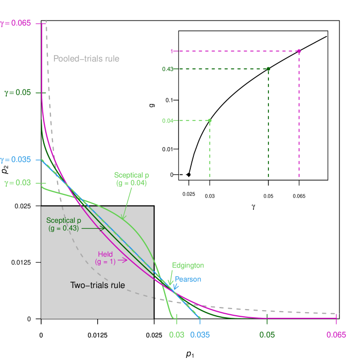
Figure 2: Success regions of different $p$-value combination methods depending on the two $p$-values $p_{1}$ and $p_{2}$. The bound on the partial T1E rate is denoted as $\gamma$. The two-trials rule success region is the squared gray area below the black line where $g=0$ and $\gamma=\alpha$. All methods control the overall T1E rate at $\alpha^{2}=0.025^{2}$, the area under each curve. The inset plot shows the dependence of the parameter $g$ of the sceptical $p$-value on the bound $\gamma$ of the partial T1E rate.

Suppose the two $p$-values $p_{1}$ and $p_{2}$ originate from two normal test statistics $Z_{i}=\Phi^{-1}(p_{i})$, $i=1,2$. Suppose further that the two trials have the same size and can be considered as exchangeable, so $\theta_{1}=\theta_{2}=\theta$. Likelihood theory then implies that $Z=Z_{1}+Z_{2}$ is sufficient for $\theta$. The pooled-trials rule (also shown in Figure 2) is based on $Z$, so will then be optimal for the test $\theta=0$ vs. $\theta>0$, i. e. under the intersection null [26]. However, this is no longer true under the union null, where $\theta_{1}\neq\theta_{2}$ is possible. As a result, the pooled-trials rule does not control the partial T1E rate at a non-trivial bound and success is possible even if one $p$-value is very large.

3.1.2 Simulation study

I now report the success probability of the different methods under different scenarios. It is well known [27] that under the alternative that was used to power the two trials, the distribution of $Z_{1}$ and $Z_{2}$ is $\operatorname{N}(\mu_{i},1)$ where $\mu_{i}=\Phi^{-1}(1-\alpha)+\Phi^{-1}(1-\beta_{i})$, where $\alpha$ is the significance threshold and $1-\beta_{i}$ the power of each trial. The case $\mu_{i}=0$ (where $\beta_{i}=1-\alpha$) represents the null hypothesis $H_{0}^{i}$: $\theta_{i}=0$.

We can thus simulate independent $Z_{1}$ and $Z_{2}$ for $\alpha=0.025$ and different values of the individual trial power $1-\beta_{i}\in\{0.9,0.8,0.6\}$ and compute the project power, the proportion of results with drug approval at overall T1E rate $\alpha^{2}=0.025^{2}$. The simulation is based on $10^{6}$ samples, so the Monte Carlo standard error is smaller than 0.05 on the percentage scale. The results shown in Table 1 are in the expected order with increasing project power for increasing bound on the partial T1E rate. The increase in project power is substantial compared to the two-trials rule. Already Edgington’s method has an increase between 3 and 5 percentage points, the sceptical $p$-value (with $g=0.43$) increases the project power by 5 to 7 percentage points. Held’s method has an even larger increase, between 6 and 8 percentage points.

We can also investigate the probability of success if one of the true treatment effects is zero (say $\mu_{1}=0$), but the other one is not. This probability cannot be larger than the bound on the partial T1E rate of the respective method and it is interesting to see how much smaller it is for different values of the power to detect the effect in the second study. The results in Table 2 show that the probability of a false positive claim has the same ordering as the project power shown in Table 1. The probabilities are fairly small, for example between 1.9 and 3.4% for the sceptical $p$-value $p_{S}$ with $g=0.43$ and upper bound 5%. Even Held’s method with a relatively large bound of 6.5% has a partial T1E rate of only 3.8% if the power of the second study is as high as 90%.

Trial power		Method
Trial 1	Trial 2	Two-trials rule	$p_{S}(c=0.04)$	Pearson	Edgington	$p_{S}(c=0.43)$	Held
90	90	81	83	84	84	86	87
90	80	72	74	76	76	78	79
90	60	54	56	59	59	61	62

Table 1: Project power of different methods for drug approval depending on individual trial power (all entries in %)

Trial power		Method
Trial 1	Trial 2	Two-trials rule	$p_{S}(c=0.04)$	Pearson	Edgington	$p_{S}(c=0.43)$	Held
Upper bound $\gamma$		2.5	3.0	3.5	3.5	5.0	6.5
NULL	90	2.2	2.5	2.9	3.0	3.4	3.8
NULL	80	2.0	2.2	2.5	2.5	2.8	3.1
NULL	60	1.5	1.6	1.8	1.8	1.9	2.1

Table 2: Partial T1E rate of different methods for drug approval depending on individual trial power (all entries in %). NULL indicates a trial with zero effect size.

3.2 Data from three trials

3.2.1 The 2-of-3 rule

Additional issues arise in the application of the two-trials rule if more than two studies are conducted [28]. Requiring two out of $n$ studies to be significant at level $\alpha$ inflates the overall T1E rate beyond $\alpha^{2}$ and so adjustments are needed. Rosenkranz [4] introduces the $k$-of-$n$ rule [see also earlier work in 17, 29] and argues that “the [overall] type-I error rate of any procedure involving more than two trials shall equal the [overall] type-I error rate from the two trials rule.” Here I consider the “2-of-3 rule” where $k=3$ studies are conducted, two of which need to be significant to flag success. Rosenkranz [4] shows that the corresponding significance level has to be reduced to $\alpha_{2|3}=0.0145$ to ensure that the overall T1E rate is $\alpha^{2}=0.025^{2}$. However, the 2-of-3 rule no longer controls the partial T1E rate, because one of the three studies can be completely unconvincing, perhaps even with an effect size estimate in the wrong direction. This is a major drawback that may be considered as unacceptable by regulators.

Furthermore, thresholding individual studies for significance without taking into account the results from the other studies creates problems in interpretation. For example, suppose that the first two studies have $p$-values $p_{1}=p_{2}=0.02$ while the third study has not yet been started. The 2-of-3 rule would then stop the project for failure, even if the standard two-trials rule (falsely assuming only two studies have been planned from the start) would flag success. Now suppose results from the third trial are also available, with $p_{3}=0.001$, say. The 2-of-3 rule would then still conclude project failure although the combined evidence for an existing treatment effect would be overwhelming. For example, the three-trials rule would flag a clear success as all three $p$-values are smaller than $0.085$ and the combined $p$-value $p=\max\{p_{1},p_{2},p_{3}\}^{3}=0.02^{3}=0.000008$ is much smaller than $0.025^{2}=0.000625$. These considerations illustrate that individual thresholding of study-specific $p$-values may lead to paradoxes that can be hard to explain to practitioners.

Nevertheless, a combined $p$-value can also be calculated for the 2-of-3 rule [30, Chapter 3], a special case of Wilkinson’s method [17]. First note that success occurs if and only if the second smallest $p$-value $p_{(2)}$ is smaller than $\alpha_{2|3}$. The second order statistic of three independent uniform distributions is known to follow a Beta $\operatorname{Be}(2,2)$ distribution, so the combined $p$-value of the 2-of-3 rule is $p=\Pr\{\operatorname{Be}(2,2)\leq p_{(2)}\}$.

3.2.2 Other methods

I now investigate the applicability of the $p$-value combination methods described in Section 2 to data from three trials. The sceptical $p$-value is not available for 3 (or more) studies, so we restrict attention to the remaining methods. Application of Held’s method to $n=3$ studies requires every study-specific $p$-value $p_{i}$ to be smaller than 0.175, as derived from (14). This is only slightly larger than the bounds 0.149 and 0.155 from Pearson’s and Edgington’s method, as listed in the last row of Table 4. These values need to be compared not to 0.025, but to $0.085$, the adjusted significance threshold of the three-trials rule. The increase in partial T1E rate of Pearson’s and Edgington’s method is therefore not more than twofold, Held’s method has a slightly larger increase.

3.2.3 Simulation study

I have conducted another simulation study with $n=3$ trials, powered at different values, now each with significance level $0.085$. The project power listed in Table 3 shows very similar values for Pearson’s, Edgington’s and Held’s method. Those values are considerably larger (nearly 10 percentage points) than for the three-trials rule. The 2-of-3 rule is also listed and has less increase in project power of around 3-6 percentage points.

Trial power			Method
Trial 1	Trial 2	Trial 3	Three-trials rule	Pearson	Edgington	Held	2-of-3 rule
90	90	90	73	81	81	82	76
90	90	80	65	74	74	74	68
90	80	60	43	52	53	53	49

Table 3: Project power of different methods for drug approval depending on individual trial power (all entries in %)

Trial power			Method
Trial 1	Trial 2	Trial 3	Three-trials rule	Pearson	Edgington	Held	2-of-3 rule
NULL	90	90	6.9	10.8	11.1	11.1	46.8
NULL	90	80	6.2	9.3	9.5	9.5	35.4
NULL	80	60	4.1	5.7	5.8	5.8	15.4
NULL	NULL	90	0.7	0.9	0.9	1.0	2.0
NULL	NULL	80	0.6	0.8	0.8	0.8	1.5
NULL	NULL	60	0.4	0.5	0.5	0.6	0.8
Upper bound			8.5	14.9	15.5	17.5	100

Table 4: Partial T1E rate of different methods for drug approval depending on individual trial power (all entries in %). NULL indicates a trial with true effect size of zero. The last row gives the upper bounds discussed in Section 3.2.2.

Turning to the partial T1E rates shown in Table 4 we see values close to 50% for the 2-of-3 rule if one of the trials comes from the null and the other two have power 90% to detect an existing effect. This illustrates the lack of control of the partial T1E rate. Pearson’s, Edgington’s and Held’s methods behave again very similar with rates between 10.8 and 11.1% in this extreme scenario. This is to be compared with 6.9% partial T1E rate for the three-trials rule.

3.2.4 Examples

We have already considered the example with $p_{1}=0.02$, $p_{2}=0.02$ and $p_{3}=0.001$, which does not lead to success with the 2-of-3 rule, which has a combined $p$-value of 0.0012. Table 5 compares this to the combined $p$-values with the different methods discussed in Section 2. All would flag success at the $\alpha_{\cap}=0.025^{2}$ level with the three-trials rule having the smallest $p$-value, orders of magnitude smaller than the combined $p$-value of the 2-of-3 rule. Table 5 also shows another example with $p_{1}=0.01$, $p_{2}=0.01$ and $p_{3}=0.2$, where the 2-of-3 rule would flag success, but all combination methods would not. Now the three-trials rule has the largest combined $p$-value. These examples illustrate that the 2-of-3 rule behaves very different than the other four methods.

$P$-values			Combined $P$-values
Trial 1	Trial 2	Trial 3	Three-trials rule	Pearson	Edgington	Held	2-of-3 rule
0.02	0.02	0.01	0.000008	0.000021	0.000021	0.000027	0.0012
0.01	0.01	0.20	0.008	0.002	0.0018	0.0031	0.0003

Table 5: Combined $p$-value with different methods for two examples with $p$-values from three trials.

4 The sequential analysis of up to three studies

Of particular interest is a sequential application of the different methods. The 2-of-3 rule has some advantages here, as it can stop for efficacy already after two studies, see Figure 3(a) for a schematic illustration. Specifically, if the first two studies are significant at level $\alpha_{2|3}$, a third trial is no longer needed and resources can be saved. Likewise, if the first two studies are both not significant, a third trial is pointless because success can never be achieved. However, there is no mechanism to stop already after the first trial, even if it is fully unconvincing.

(a) The 2-of-3 rule

(b) Edgington’s method

(c) Sequential Edgington’s method

Figure 3: The 2-of-3 rule and Edgington’s method to analyse three trials sequentially. The two-of-three rule requires the adjusted significance level $\alpha_{2|3}=0.015$ at overall T1E rate $\alpha_{\cap}=0.025^{2}$. Success with Edgington’s method requires $E_{3}=\sum_{i=1}^{3}p_{i}$ to be not larger than the “budget” $0.16$. Failure occurs as soon as $E_{k}=\sum_{i=1}^{k}p_{i}>{\color[rgb]{0,0,0}0.16}$ for some $k=1,2,3$. The budget is reduced to 0.11 in the sequential application of Edgington’s method with $q=0.72$ to be able to stop for success after 2 trials if $p_{1}+p_{2}\leq 0.03$.

4.1 Early stopping for failure

All methods that control the partial T1E rate at a non-trivial bound can stop for failure already after the first and second trial, as illustrated in Figure 3(b) for Edgington’s method. However, to achieve success these methods always need three trials. This is because they are all based on a “budget” $a_{3}$, $b_{3}$ resp. $c_{3}$ and the results from the three trials need to be “within budget”:

$$K_{3}=\sum_{i=1}^{3}-2\log(1-p_{i}) \leq a_{3}\mbox{ (Pearson), }$$

$$E_{3}=\sum_{i=1}^{3}p_{i} \leq b_{3}\mbox{ (Edgington), }$$

$$H_{3}=\sum_{i=1}^{3}1/Z_{i}^{2} \leq c_{3}\mbox{ (Held). }$$

A very convincing trial will cost only very little and will reduce the budget only little. On the other hand, an unconvincing first trial is likely to overspend the budget so success will be impossible, no matter what the results of the remaining two studies will be. We can hence stop the project for failure and there is no need to conduct the second and third study. Likewise, if the budget is overspent after the second trial, there is no need to conduct the third study.

What is different with the three methods is the “currency”, either the “price” of a trial is given in $-2\log(1-p_{i})$ (Pearson) or $p_{i}$ (Edgington) or $1/Z_{i}^{2}$ (Held). This gives different weights for different $p$-values, as shown in Figure 4, where the price of a single study is normalized to a “unit budget”. The Figure shows that the price of Pearson’s method is close to Edgington’s method, so nearly linear. In contrast, Held’s method has higher prices of convincing studies with small $p$-values, while less convincing studies are “cheaper”. The difference between Held’s and the other methods is larger for $n=2$ than for $n=3$ studies.

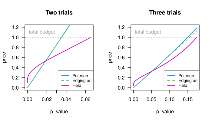
Figure 4: The price of a single study for Pearson’s, Edgington’s and Held’s method as a function of the one-sided $p$-value. The price is normalized to a unit total budget (the dashed horizontal line) for $n=2$ (left) and $n=3$ (right) trials at overall T1E level $\alpha_{\cap}=0.025^{2}$.

Possible decisions after two trials are shown in the left panel of Figure 5 for the different methods considered and compared to the three-trials rule. Remarkably, the area where the three-trials rule continues to the third study is considerably smaller than for the other three methods. Held’s method will always continue with a third study if the three-trials rule does so, but may also continue if the three-trials rule doesn’t.

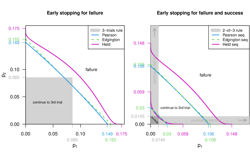
Figure 5: Possible decisions with Pearson’s, Edgington’s and Held’s method after two studies with one-sided $p$-values $p_{1}$ and $p_{2}$ have been conducted. The non-sequential procedures (left) will stop for failure if the point $(p_{1},p_{2})$ is above the respective line, otherwise a third trial will be conducted. The grey areas indicate the corresponding continuation region of the three-trials rule. The sequential procedures (right) are indicated with two lines in the same color and will stop for failure if the point $(p_{1},p_{2})$ is above the upper line. They will stop for success if the point is below the lower line. If the point is between the upper and lower line, an additional third trial will be conducted. The grey areas indicate the corresponding success and continuation regions of the 2-of-3 rule.

4.2 Early stopping for failure and success

Sequential application of one of the methods will also allow to stop for success after 2 studies. Adjusted significance levels $\alpha_{2}$ and $\alpha_{3}$ for the tests after two and three studies, respectively, then have to be chosen such that the overall T1E rate is equal to $\alpha_{\cap}=\alpha^{2}$. The level $\alpha_{2}=q\,\alpha_{\cap}$ will be a proportion $q$ of $\alpha_{\cap}$, following the theory of group-sequential methods [27, Section 8.2]. Of course, the more lenient we are after the second study, the more strict we have to be after the third. I will choose $q=0.72$ throughout to allow for a 20% increase of the partial T1E rate to 0.03 for Edgington’s method and $n=2$ trials, but of course other choices can be made. Sequential application with $q=0.72$ is illustrated in Figure 3(c). As in the non-sequential version, stopping for failure after Trial 1 or Trial 2 is possible, but now also stopping for success after two trials.

Computation of the adjusted level $\alpha_{3}$ to be used after results from all three trials are available can be done as in group-sequential trials [27, Section 8.2.2] based on the factorization

$$K_{3} = K_{2}-2\log(1-p_{3})$$ (15)

$$E_{3} = E_{2}+p_{3}$$ (16)

$$H_{3} = H_{2}+1/Z_{3}^{2}$$ (17)

for Pearson’s, Edgington’s and Held’s method, respectively. The two terms on the right-hand side of each equation are independent with known distributions under the intersection null. A convolution can be therefore used to compute the distribution of $K_{3}$, $E_{3}$ and $H_{3}$, respectively, conditional on no success after two studies. This can then be used to compute the adjusted level $\alpha_{3}$ shown in Table 6, details are given in Appendix A. Table 6 also gives the corresponding partial T1E bounds $\gamma_{2}$ resp. $\gamma_{3}$ for the sequential methods, which are smaller than for the non-sequential methods.

	$q$	$\alpha_{2}$	$\alpha_{3}$	$\gamma_{2}$	$\gamma_{3}$
Two-trials rule	1	$0.025^{2}$		0.025
Three-trials rule	0		$0.025^{2}$		0.085
Pearson 2 trials	1	$0.025^{2}$		0.035
Pearson 3 trials	0		$0.025^{2}$		0.15
Pearson sequential	0.72	$0.0212^{2}$	$0.0146^{2}$	$0.0298$	$0.106$
Edgington 2 trials	1	$0.025^{2}$		0.035
Edgington 3 trials	0		$0.025^{2}$		0.16
Edgington sequential	0.72	$0.0212^{2}$	$0.0147^{2}$	$0.030$	$0.109$
Held 2 trials	1	$0.025^{2}$		0.065
Held 3 trials	0		$0.025^{2}$		0.17
Held sequential	0.72	$0.0212^{2}$	$0.0147^{2}$	$0.059$	$0.148$

Table 6: Adjusted significance levels $\alpha_{i}$ and partial T1E bounds $\gamma_{i}$, $i=2,3$, for the two- and three-trials rule, Pearson’s, Edgington’s and Held’s method, including sequential versions of the latter three.

4.2.1 Possible decisions after the first trial

It is interesting that the sequential versions give three (rather than just two) options how to proceed after the first study has been conducted. This is illustrated in Figure 6 for Edgington’s and Held’s method and $q=0.72$, Pearson’s method will be very similar to Edgington’s method. As we can see, the three options are stopping for failure if $p_{1}>\gamma_{3}$, continuing with a second trial (if $p_{1}\leq\gamma_{2}$) or continuing directly with a second and third trial, perhaps even in parallel. The last category is chosen, if the $p$-value of the first study is only “suggestive” in the sense that a second trial will never lead to success but a second and a third trial may do. Formally this is achieved if $\gamma_{2}<p_{1}\leq\gamma_{3}$.

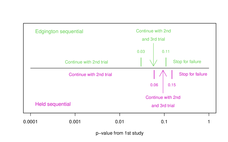
Figure 6: Possible decisions based on the $p$-value $p_{1}$ from the first trial and the sequential Edgington’s resp. Held’s method. Both methods control the overall T1E rate at $\alpha_{\cap}=0.025^{2}$ and spend the proportion $q=0.72$ of $\alpha_{\cap}$ on $\alpha_{2}$.

4.2.2 Possible decisions after the second trial

The possible decisions of sequential methods (with $q=0.72$) after the second trial are displayed in the right panel of Figure 5. Now there is the additional possibility that the procedures can stop for success. As a result, the failure regions are somewhat larger than in the non-sequential versions. The 2-of-3 rule is also displayed and has a very different success, continuation and failure region. Note that the 2-of-3 continuation region extends up to one, so to a larger area than shown, as long as one $p$-value is sufficiently small ($<0.0145$).

4.3 Operating characteristics

Figure 7 compares operating characteristics of the different methods for data from 3 trials based on a simulation with $10^{7}$ samples. Each individual trial has been powered at the standard significance level 0.025 with varying power between 2.5% (where $\mu_{i}=0$) and 97.5%. The left figure gives the difference in success rate compared to the three-trials rule. It shows that most of the methods have increased project power, the largest is obtained for the non-sequential versions, where Held’s and Edgington’s method are slightly better than Pearson’s. The sequential version show smaller improvements compared to the three-trials rule, now with a more pronounced advantage of Held’s method due to the substantially larger bound on the partial T1E rate for 2 trials. The 2-of-3 rule has less project power than the three-trials rule, if the individual trials are underpowered, but more power if the trials are reasonably powered.

The right panel of Figure 7 gives the expected number of trials required before the project is stopped. If the power is low, the 2-of-3 rule has the largest expected number of studies required. All other methods can stop for failure already after trial 1, so the expected number of trials is between 1 and 2 for underpowered studies. If the power is large, the non-sequential methods require the largest number of studies on average, because they require three studies to be conducted to reach success. The sequential methods of Pearson’s, Edgington’s and Held’s method require a smaller number of studies, never larger than around 2.2 studies on average. Of course, all these results are based on a fixed proportion $q=0.72$ of overall T1E rate spent after the second study. It remains to be investigated which choice of $q$ gives optimal operating characteristics in terms of project power or expected number of trials.

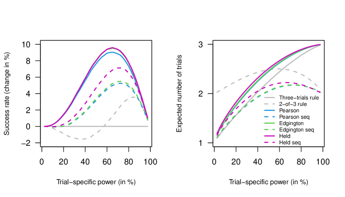
Figure 7: Success rate (left, change in % compared to the three-trials rule) and number of trials needed (right) for the different methods as a function of trial-specific power.

5 Discussion and Outlook

Alternatives to the two-trials rule require appropriate T1E control, both overall and partial. I have described and compared different $p$-value combination methods that have the same overall T1E rate, offer partial T1E control at a non-trivial bound and can be extended to a sequential assessment of success. The methods have different properties and a particular one can be chosen based on a desired bound on the partial T1E rate. Edgington’s method based on the sum of the $p$-values has the advantage that it is easy to implement and communicate, has only moderate partial Type-I error rate inflation but still substantially increased project power compared to the two- and three-trials rule, respectively. Of course, to guarantee exact overall T1E rate control, the specific type of combination method, whether fixed or sequential as well as the maximum number of studies conducted have to be defined in advance of the project in a “master protocol”. This may be considered a limitation from a study conduct point of view [4].

A related question is how acceptable it is by regulators to have inflated partial T1E. Johnston et al. [31] systematically investigated the frequency of and rationale for FDA approval of drugs based on pivotal trials with non-significant (“null”) findings. Among 210 new drugs approved between 2018 and 2021 they identified 21 (10%) not meeting pivotal trial endpoints. 15 were based on more than 1 pivotal study and the most common reported rationale for FDA approval was “success of other primary end points in pivotal study” (13 drugs). This implies that regulators do implicitly allow for some partial T1E rate inflation as long as there is another successful (i.e. conventionally significant) trial. The proposed methods in this paper formalize this rationale for drug approval, requiring overall T1E control at $\alpha^{2}$ while allowing for a partial T1E rate somewhat larger than $\alpha$.

In the simulations presented I have assumed that the sample size of each trial was calculated in advance based on a certain power $1-\beta$ to detect a pre-specified clinically relevant difference. It was shown that the methods described have larger project power than the two- and three trials rule, respectively. One may also ask how much the sample size of two trials can be reduced to achieve the project power $(1-\beta)^{2}$ of the two-trials rule. The possible reduction in sample size is around 6% for Edgington’s rule (see Appendix C), for the other methods even larger.

The different methods also allow to compute the sample size adaptively based on the results from the previous trial [32]. For example, we could design a second trial to detect the observed effect from the first trial with a certain power [33]. This will be particularly simple for Edgington’s method, where the required significance level is $b_{2}-p_{1}$, but also straightforward for the other approaches. A comparison of the expected number of patients needed under the different procedures could be done and the conditional T1E rate could be investigated [8, Section 3.4]. We may also compute the conditional (or predictive) power to reach success given the results from an initial trial. The bound on the partial T1E rate can directly be used to describe when this power is exactly zero and when not. But even if conditional power is non-zero it can be too small to warrant a further trial.

It is also possible to adopt the sequential methods such that a stop for success already after the first study would be possible. This would incorporate the argument brought forward by Fisher [34] that one large and very convincing trial may give sufficient evidence of efficacy. Also Kay [35] notes that “where there are practical reasons why two trials cannot be easily undertaken or where there is a major unfulfilled public health need, it may be possible for a claim to be based on a single pivotal trial.” The notion of replicability could then be enforced in a post-marketing requirement after conditional or accelerated drug approval [32]. However, it is well-known from group-sequential methods, that the $p$-value obtained after stopping for success overstates the evidence against the null and some adjustment is required [36].

Finally, regulators are also interested in a combined effect estimate with confidence interval to assess whether the project has demonstrated a clinically meaningful effect [2]. $P$-value combination methods can be inverted to obtain a confidence interval for the effect estimate based on the corresponding $p$-value function [37]. In future work we will compare the different methods, for example in terms of coverage and width of the resulting confidence intervals. We will also investigate how they need to be adopted to the sequential setting, where the standard combined effect estimate in group-sequential trials is known to be biased if we stop early for success [38].

Code

Code to reproduce the calculations in this manuscript is available at https://osf.io/3pgmk/.

Acknowledgments

Support by the Swiss National Science Foundation (Project # 189295) is gratefully acknowledged. I appreciate helpful comments by Charlotte Micheloud, Samuel Pawel, Frank Pétavy and Kit Roes. I am grateful for comments by two referees on an earlier version of this paper.

Appendix A Details on sequential application

A.1 Pearson’s method

The adjusted level $\alpha_{2}=q\cdot\alpha_{\cap}$ with budget $a_{2}=\chi^{2}_{4}(\alpha_{2})$ is chosen to spend the proportion $q$ of $\alpha_{\cap}$ on $\alpha_{2}$. To compute the adjusted level $\alpha_{3}$ such that the overall T1E rate is $\alpha_{\cap}$ we need the distribution of $K_{3}\,|\,\{K_{2}>a_{2}\}$ where $K_{n}$ is defined in (6). The condition $K_{2}>a_{2}$ is needed, because the assessment of success after $3$ studies requires that there was no success after $2$ studies. Due to (15), the density $f(k_{3}\,|\,\{K_{2}>a_{2}\})$ can be obtained by a convolution of the density of $K_{2}\,|\,\{K_{2}>a_{2}\}$ and the density of $-2\log(1-p_{3})\sim\operatorname{Ga}(1,1/2)$, a gamma distribution with shape and rate parameters 1 and $1/2$. The density of $K_{2}\,|\,\{K_{2}>a_{2}\}$ is a $\operatorname{Ga}(2,1/2)$ density truncated to $K_{2}>a_{2}$, which occurs with probability $1-\Pr(K_{2}\leq a_{2})=1-\alpha_{2}$:

$$f(k_{2}\,|\,\{K_{2}>a_{2}\})=\frac{1}{1-\alpha_{2}}\operatorname{Ga}(k_{2};2,1/2){\mathbf{1}}_{\{k_{2}>a_{2}\}},$$

now $\operatorname{Ga}(x;a,b)$ denotes the density of the gamma distribution at $x$ with shape parameter $a$ and rate parameter $b$.

The convolution of $K_{2}\,|\,\{K_{2}>a_{2}\}$ and $-2\log(1-p_{3})$ therefore has density

$$f(k_{3}\,|\,\{K_{2}>a_{2}\})=\left\{\begin{array}[]{ll}\frac{1}{1-\alpha_{2}}\int\limits_{a_{2}}^{k_{3}}\operatorname{Ga}(x;2,1/2)\operatorname{Ga}(k_{3}-x;1,1/2)dx&\mbox{ if }k_{3}>a_{2}\\ 0&\mbox{ else.}\end{array}\right.$$

Numerical integration of $f(k_{3}\,|\,\{K_{2}>a_{2}\})$ can be used to compute the cumulative distribution function

$$F(k_{3}\,|\,\{K_{2}>a_{2}\})=\Pr(K_{3}\leq k_{3}\,|\,\{K_{2}>a_{2}\}).$$ (18)

Root-finding methods are then used to determine the adjusted level $\alpha_{3}$ with budget $\chi^{2}_{6}(\alpha_{3})$ such that $F(a_{3}\,|\,\{K_{2}>a_{2}\})=\alpha_{\cap}-\alpha_{2}=(1-q)\cdot\alpha_{\cap}$ holds.

A.2 Edgington’s method

The adjusted level $\alpha_{2}=q\cdot\alpha_{\cap}$ with budget $b_{2}=\sqrt{2\alpha_{2}}$ is chosen to spend the proportion $q$ of $\alpha_{\cap}$ on $\alpha_{2}$. To compute the adjusted level $\alpha_{3}$ such that the overall T1E rate is $\alpha_{\cap}$ we need the distribution of $E_{3}\,|\,\{E_{2}>b_{2}\}$ where $E_{n}$ is defined in (9). Due to (16), the density $f(e_{3}\,|\,\{E_{2}>b_{2}\})$ can be obtained by a convolution of the density of $E_{2}\,|\,\{E_{2}>b_{2}\}$ and the density of $p_{3}\sim\operatorname{U}(0,1)$. The density of the first term is a Irwin-Hall density truncated to $E_{2}>b_{2}$, which occurs with probability $1-\Pr(E_{2}\leq b_{2})=1-\alpha_{2}$:

$$f(e_{2}\,|\,\{E_{2}>b_{2}\})=\frac{1}{1-\alpha_{2}}\operatorname{IH}(e_{2};n=2){\mathbf{1}}_{\{e_{2}>b_{2}\}},$$

here $\operatorname{IH}(x;n)$ denotes the density of the Irwin-Hall distribution with parameter $n$. For $n=2$ this is

$$\operatorname{IH}(x;n=2)=\left\{\begin{array}[]{rl}x&\mbox{ for }0\leq x<1,\\ 2-x&\mbox{ for }1\leq x\leq 2.\end{array}\right.$$ (19)

The convolution of $E_{2}\,|\,\{E_{2}>b_{2}\}$ and $p_{3}$ therefore has density

$$f(e_{3}\,|\,\{E_{2}>b_{2}\})=\left\{\begin{array}[]{ll}\frac{1}{1-\alpha_{2}}\int\limits_{b_{2}}^{e_{3}}\operatorname{IH}(x;2)dx&\mbox{ if }e_{3}>b_{2}\\ 0&\mbox{ else.}\end{array}\right.$$

Note that the integral $\int\limits_{b_{2}}^{e_{3}}\operatorname{IH}(x;2)dx=\int\limits_{0}^{e_{3}}\operatorname{IH}(x;2)dx-\int\limits_{0}^{b_{2}}\operatorname{IH}(x;2)dx$ can be easily calculated based on the cdf of the $\operatorname{IH}(2)$ distribution, which is analytically available from (19). Numerical integration of $f(e_{3}\,|\,\{E_{2}>b_{2}\})$ finally gives the cumulative distribution function

$$F(e_{3}\,|\,\{E_{2}>b_{2}\})=\Pr(E_{3}\leq e_{3}\,|\,\{E_{2}>b_{2}\}).$$ (20)

Root-finding methods are then used to determine the adjusted level $\alpha_{3}$ with budget $b_{3}=\sqrt[3]{6\alpha_{3}}$ such that $F(b_{3}\,|\,\{E_{2}>b_{2}\})=\alpha_{\cap}-\alpha_{2}=(1-q)\cdot\alpha_{\cap}$ holds.

A.3 Held’s method

The adjusted level $\alpha_{2}=q\cdot\alpha_{\cap}$ with budget $c_{2}=4/\left[\Phi^{-1}(1-2\alpha_{2})\right]^{2}$ is chosen to spend the proportion $q$ of $\alpha_{\cap}$ on $\alpha_{2}$. To compute the adjusted level $\alpha_{3}$ such that the overall T1E rate is $\alpha_{\cap}$ we need the distribution of $H_{3}\,|\,\{H_{2}>c_{2}\}$ where $H_{n}$ is defined in (13). Due to (17), the density $f(h_{3}\,|\,\{H_{2}>c_{2}\})$ can be obtained by a convolution of the density of $H_{2}\,|\,\{H_{2}>c_{2}\}$ and the density of $1/Z_{3}^{2}\sim\operatorname{IG}(1/2,1/2)$, an inverse gamma distribution. The density of the first term is an $\operatorname{IG}(1/2,2)$ density truncated to $H_{2}>c_{2}$, which occurs with probability $1-\Pr(H_{2}\leq c_{2})=1-4\,\alpha_{2}$ (the factor 4 enters here because $H_{2}$ doesn’t take the signs of $Z_{1}$ and $Z_{2}$ into account):

$$f(h_{2}\,|\,\{H_{2}>c_{2}\})=\frac{1}{1-4\,\alpha_{2}}\operatorname{IG}(h_{2};1/2,2){\mathbf{1}}_{\{h_{2}>c_{2}\}},$$

now $\operatorname{IG}(x;a,b)$ denotes the density of the inverse gamma distribution at $x$ with shape parameter $a$ and rate parameter $b$:

$$\operatorname{IG}(x;a,b)=\left\{\begin{array}[]{rl}\frac{b^{a}}{\Gamma(a)}x^{-(a+1)}\exp(-b/x)&\mbox{ for }x>0\\ 0&\mbox{ else. }\end{array}\right.$$

The convolution of $H_{2}\,|\,\{H_{2}>c_{2}\}$ and $1/Z_{3}^{2}$ therefore has density

$$f(h_{3}\,|\,\{H_{2}>c_{2}\})=\left\{\begin{array}[]{ll}\frac{1}{1-4\alpha_{2}}\int\limits_{c_{2}}^{h_{3}}\operatorname{IG}(x;1/2,2)\operatorname{IG}(h_{3}-x;1/2,1/2)dx&\mbox{ if }h_{3}>c_{2}\\ 0&\mbox{ else.}\end{array}\right.$$

Numerical integration of $f(h_{3}\,|\,\{H_{2}>c_{2}\})$ can be used to compute the cumulative distribution function

$$F(h_{3}\,|\,\{H_{2}>c_{2}\})=\Pr(H_{3}\leq h_{3}\,|\,\{H_{2}>c_{2}\}).$$ (21)

Root-finding methods are then used to determine the adjusted level $\alpha_{3}$ with budget $c_{3}=9/\left[\Phi^{-1}(1-4\alpha_{3})\right]^{2}$ such that $F(c_{3}\,|\,\{H_{2}>c_{2}\}){\color[rgb]{0,0,0}/8}=\alpha_{\cap}-\alpha_{2}=(1-q)\cdot\alpha_{\cap}$ holds. Division by $2^{3}=8$ is required because $H_{3}$ doesn’t take the signs of $Z_{1}$, $Z_{2}$ and $Z_{3}$ into account.

Appendix B Stopping Probabilities

Figure 8 shows for the different approaches the probability to stop after the first, second or third trial as a function of the power of the individual trials varying between 2.5 and 97.5%. The three-trials and 2-of-3 rule offers no possibility to stop after the first trial, so only two lines are shown.

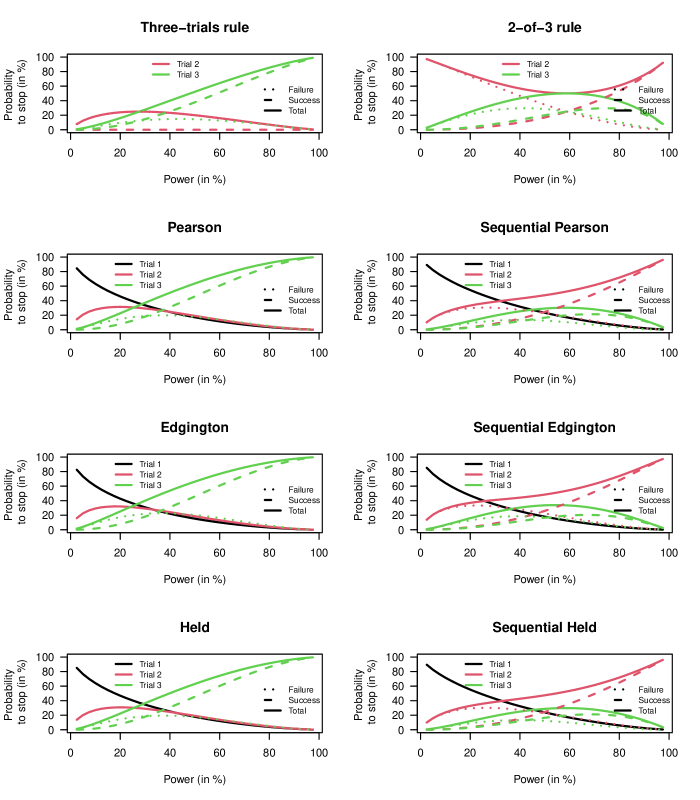
Figure 8: Probabilities to stop after the different trials. Dotted lines represent stopping for failure. Dashed lines represent stopping for success. Solid lines represent stopping for either failure or success.

Appendix C Sample size reduction of Edgington’s method

Suppose two trials are powered at significance level $\alpha$ with individual trial power $1-\beta$. The distribution of the the sum of the two $p$-values can then be derived as the convolution of the distribution of the two $p$-values under the alternative [39], which can be used to compute the project power of Edgington’s method numerically. Root-finding methods can then be applied to find the power $1-\beta^{\prime}$ that achieves the project power $(1-\beta)^{2}$ of the two-trials rule. The relative sample size then is

$$\frac{n^{\prime}}{n}=\left\{\frac{\Phi^{-1}(1-\alpha)+\Phi^{-1}(1-\beta^{\prime})}{\Phi^{-1}(1-\alpha)+\Phi^{-1}(1-\beta)}\right\}^{2}$$

and the sample size reduction is $1-n^{\prime}/n$. Figure 9 shows that the reduction is fairly constant around 6% for a wide range of values of the project power $(1-\beta)^{2}$.

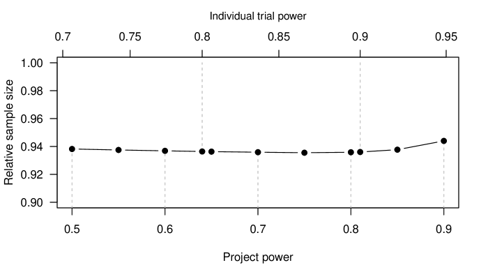
Figure 9: Relative sample size required to achieve the same project power as the two-trials rule with Edgington’s method.

References

- FDA [1998] FDA. Providing clinical evidence of effectiveness for human drug and biological products, 1998. www.fda.gov/regulatory-information/search-fda-guidance-documents/providing-clinical-evidence-effectiveness-human-drug-and-biological-products.
- FDA [2019] FDA. Substantial evidence of effectiveness for human drug and biological products, 2019. https://www.fda.gov/drugs/guidance-compliance-regulatory-information/guidances-drugs.
- Senn [2021] S. Senn. Statistical Issues in Drug Development. John Wiley & Sons, Chichester, U.K., third edition, 2021.
- Rosenkranz [2023] G. K. Rosenkranz. A generalization of the two trials paradigm. Therapeutic Innovation & Regulatory Science, 57:316–320, 2023. URL https://doi.org/10.1007/s43441-022-00471-4.
- Sonnemann [1991] E. Sonnemann. Kombination unabhängiger Tests. In Jürgen Vollmar, editor, Biometrie in der chemisch-pharmazeutischen Industrie 4, pages 91–112. Fischer Verlag, 1991. in German.
- Shun et al. [2005] Z. Shun, E. Chi, S. Durrleman, and L. Fisher. Statistical consideration of the strategy for demonstrating clinical evidence of effectiveness—one larger vs two smaller pivotal studies. Statistics in Medicine, 24(11):1619–1637, 2005. 10.1002/sim.2018. URL https://onlinelibrary.wiley.com/doi/abs/10.1002/sim.2018.
- Heller et al. [2014] R. Heller, M. Bogomolov, and Y. Benjamini. Deciding whether follow-up studies have replicated findings in a preliminary large-scale omics study. Proceedings of the National Academy of Sciences, 111(46):16262–16267, 2014. 10.1073/pnas.1314814111. URL https://www.pnas.org/doi/abs/10.1073/pnas.1314814111.
- Micheloud et al. [2023] C. Micheloud, F. Balabdaoui, and L. Held. Assessing replicability with the sceptical -value: Type-I error control and sample size planning. Statistica Neerlandica, 77:573–591, 2023. https://doi.org/10.1111/stan.12312.
- Zhan et al. [2023] S. J. Zhan, C. U. Kunz, and N. Stallard. Should the two-trial paradigm still be the gold standard in drug assessment? Pharmaceutical Statistics, 22:96–111, 2023. https://doi.org/10.1002/pst.2262. URL https://onlinelibrary.wiley.com/doi/abs/10.1002/pst.2262.
- Rubin [1992] D. B. Rubin. Meta-analysis: literature synthesis or effect-size surface estimation? Journal of Educational Statistics, 17(4):363–374, 1992.
- Cousins [2008] Robert D. Cousins. Annotated bibliography of some papers on combining significances or p-values, 2008. https://arxiv.org/abs/0705.2209.
- Stouffer et al. [1949] S. A. Stouffer, E. A. Suchman, L. C. Devinney, S. A. Star, and Jr. Williams, R. M. The American soldier: Adjustment during army life. (Studies in social psychology in World War II). Cambridge University Press, Princeton Univ. Press, 1949.
- Senn [1997] S. Senn. Statistical Issues in Drug Development. John Wiley & Sons, Chichester, U.K., first edition, 1997.
- Bauer and Köhne [1994] P. Bauer and K. Köhne. Evaluation of experiments with adaptive interim analyses. Biometrics, 50:1029–1041, 1994. URL http://www.jstor.org/stable/2533441.
- Rosenkranz [2002] G. Rosenkranz. Is it possible to claim efficacy if one of two trials is significant while the other just shows a trend? Drug Information Journal, 36(1):875–879, 2002. URL https://doi.org/10.1177/009286150203600416.
- Edgington [1972] E. S. Edgington. An additive method for combining probability values from independent experiments. The Journal of Psychology, 80:351–363, 1972.
- Wilkinson [1951] B. Wilkinson. A statistical consideration in psychological research. Psychological Bulletin, 48:156–157, 1951. 10.1037/h0059111.
- Pearson [1933] K. Pearson. On a method of determining whether a sample of size n supposed to have been drawn from a parent population having a known probability integral has probably been drawn at random. Biometrika, 25:379–410, 1933. URL http://www.jstor.org/stable/2332290.
- Pearson [1934] K. Pearson. On a new method of determining "goodness of fit". Biometrika, 26:425–442, 1934. URL http://www.jstor.org/stable/2331988.
- Fisher [1932] R. A. Fisher. Statistical Methods for Research Workers. Oliver & Boyd, Edinburgh, 4th ed. edition, 1932.
- Irwin [1927] J. O. Irwin. On the frequency distribution of the means of samples from a population having any law of frequency with finite moments, with special reference to Pearson’s Type II. Biometrika, 19(3-4):225–239, 12 1927. ISSN 0006-3444. 10.1093/biomet/19.3-4.225. URL https://doi.org/10.1093/biomet/19.3-4.225.
- Hall [1927] P. Hall. The distribution of means for samples if size drawn from a population in which the variate takes values between 0 and 1, all such values being equally probable. Biometrika, 19(3-4):240–244, 12 1927. ISSN 0006-3444. 10.1093/biomet/19.3-4.240. URL https://doi.org/10.1093/biomet/19.3-4.240.
- Johnson et al. [1995] N. L. Johnson, S. Kotz, and N. Balakrishnan. Continuous Univariate Distributions, Volume 2, volume 2. Wiley, New York, 2 edition, 1995.
- Held [2020a] L. Held. The harmonic mean -test to substantiate scientific findings. Journal of the Royal Statistical Society, Series C, 69(3):697–708, 2020a.
- Held [2020b] L. Held. A new standard for the analysis and design of replication studies (with discussion). Journal of the Royal Statistical Society, Series A, 183:431–469, 2020b.
- Maca et al. [2002] J. Maca, P. Gallo, M. Branson, and W. Maurer. Reconsidering some aspects of the two-trials paradigm. Journal of Biopharmaceutical Statistics, 12(2):107–119, jan 2002. 10.1081/bip-120006450. URL https://doi.org/10.1081/bip-120006450.
- Matthews [2006] J. N. S. Matthews. Introduction to Randomized Controlled Clinical Trials. Chapman & Hall/CRC, second edition, 2006.
- Fisher [1999a] L. D. Fisher. Carvedilol and the Food and Drug Administration (FDA) approval process: The FDA paradigm and reflections on hypothesis testing. Controlled Clinical Trials, 20(1):16–39, 1999a. ISSN 0197-2456. https://doi.org/10.1016/S0197-2456(98)00054-3. URL http://www.sciencedirect.com/science/article/pii/S0197245698000543.
- Rüger [1978] B. Rüger. Das maximale Signifikanzniveau des Tests: "Lehne ab, wenn unter gegebenen Tests zur Ablehnung führen". Metrika, 25:171–178, 1978.
- Hedges and Olkin [1985] Larry V. Hedges and Ingram Olkin. Statistical Methods for Meta-Analysis. Elsevier, 1985. 10.1016/c2009-0-03396-0.
- Johnston et al. [2023] J. L. Johnston, J. S. Ross, and R. Ramachandran. US Food and Drug Administration Approval of Drugs Not Meeting Pivotal Trial Primary End Points, 2018-2021. JAMA Internal Medicine, 183(4):376–380, 04 2023. ISSN 2168-6106. 10.1001/jamainternmed.2022.6444. URL https://doi.org/10.1001/jamainternmed.2022.6444.
- Deforth et al. [2023] M. Deforth, C. Micheloud, K. Roes, and L. Held. Combining evidence from clinical trials in conditional or accelerated approval. Pharmaceutical Statistics, 22:707–720, 2023. https://doi.org/10.1002/pst.2302.
- Micheloud and Held [2022] C Micheloud and L Held. Power calculations for replication studies. Statistical Science, 37(3):369–379, 2022. 10.1214/21-STS828. URL https://doi.org/10.1214/21-STS828.
- Fisher [1999b] L. D. Fisher. One large, well-designed, multicenter study as an alternative to the usual FDA paradigm. Drug Information Journal, 33(1):265––271, 1999b. URL https://doi.org/10.1177/009286159903300130.
- Kay [2015] R. Kay. Statistical Thinking for Non-Statisticians in Drug Regulation. John Wiley & Sons, Chichester, U.K., second edition, 2015. https://doi.org/10.1002/9781118451885.
- Cook [2002] T. D. Cook. P-value adjustment in sequential clinical trials. Biometrics, 58:105–11, 2002. URL http://www.jstor.org/stable/3068544.
- Infanger and Schmidt-Trucksäss [2019] D. Infanger and A. Schmidt-Trucksäss. P value functions: An underused method to present research results and to promote quantitative reasoning. Statistics in Medicine, 38(21):4189–4197, 2019. 10.1002/sim.8293. URL https://onlinelibrary.wiley.com/doi/abs/10.1002/sim.8293.
- Pinheiro and DeMets [1997] J. C. Pinheiro and D. L. DeMets. Estimating and reducing bias in group sequential designs with Gaussian independent increment structure. Biometrika, 84:831–845, 1997.
- Hung et al. [1997] H M J Hung, R T O’Neill, P Bauer, and K Köhne. The behavior of the -value when the alternative hypothesis is true. Biometrics, 53(1):11–22, 1997.