QBitOpt: Fast and Accurate Bitwidth Reallocation during Training

Abstract

Quantizing neural networks is one of the most effective methods for achieving efficient inference on mobile and embedded devices. In particular, mixed precision quantized (MPQ) networks, whose layers can be quantized to different bitwidths, achieve better task performance for the same resource constraint compared to networks with homogeneous bitwidths. However, finding the optimal bitwidth allocation is a challenging problem as the search space grows exponentially with the number of layers in the network. In this paper, we propose QBitOpt, a novel algorithm for updating bitwidths during quantization-aware training (QAT). We formulate the bitwidth allocation problem as a constraint optimization problem. By combining fast-to-compute sensitivities with efficient solvers during QAT, QBitOpt can produce mixed-precision networks with high task performance guaranteed to satisfy strict resource constraints. This contrasts with existing mixed-precision methods that learn bitwidths using gradients and cannot provide such guarantees. We evaluate QBitOpt on ImageNet and confirm that we outperform existing fixed and mixed-precision methods under average bitwidth constraints, commonly found in literature.

1 Introduction

In the last decade, neural networks have driven some of the most significant advances in artificial intelligence. However, searching for better-performing neural networks has increased their resource requirements substantially. The increase in parameters and training time is most notable in transformer models that are becoming ubiquitous in computer vision [12, 39] and natural language understanding [34, 5]. As a result, deploying these ever-growing neural networks on resource-constrained devices, such as mobile phones, embedded systems, and IoT devices, remains a challenge. Quantization has been proven to be a very effective method of addressing this constraint by reducing the memory and computational cost of neural networks without sacrificing their accuracy [22, 26, 29]. This is achieved by compressing the floating-point weights and activation to a more efficient low bitwidth fixed-point representation. Deploying quantizing neural networks on devices is also becoming easier as increasing numner of devices support efficient low-precision operation.

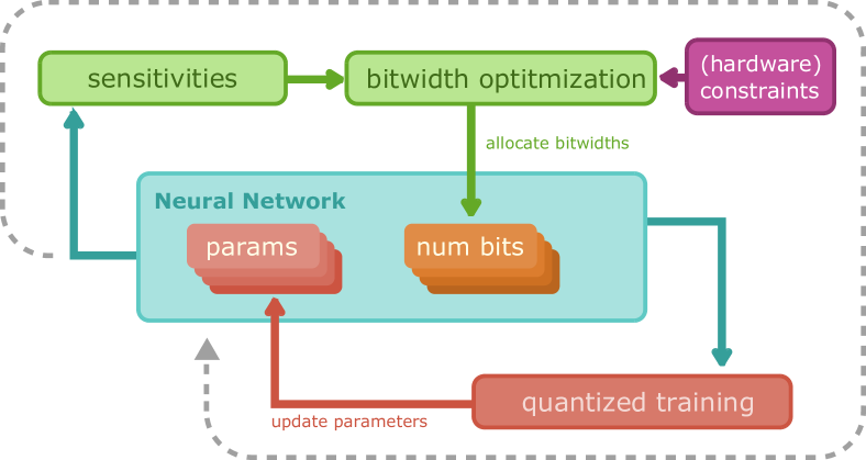
Figure 1: QBitOpt uses a quantization sensitivity metric to infer bitwidths while taking (hardware) constraints into account. The bitwidth allocation is used within a QAT training loop.

Neural network quantization is an active field of research, and various methods have emerged in recent years. Broadly, we can distinguish them into two main groups: post-training quantization (PTQ) [31, 43, 28, 15, 27, 16], and quantization-aware training (QAT) [24, 14, 25, 30, 40, 23]. In PTQ, we take a pre-trained neural network as input and infer the quantization setting that maximizes task performance without access to labeled data or the original training pipeline. In contrast, in QAT, we simulate quantization during training and allow the network parameters to adjust to quantization noise. In both cases, the target quantization bitwidth is commonly determined beforehand and is set homogeneously over the entire network. A crucial drawback of this approach is that the homogeneous bitwidth can only be as low as the network’s most sensitive layer allows.

However, not all layers in a neural network are equally sensitive to quantization. Hence, it is beneficial to quantize some layers at a higher bitwidth than others. For example, it is common in quantization literature [14, 23, 13, 30] to keep the first and last layer of a neural network at a higher bitwidth than the rest of the network because it improves accuracy with only an incremental increase in resource requirements. Allowing for a heterogeneous bitwidth allocation across the layers of a neural network is called mixed-precision quantization (MPQ). The main challenge of MPQ algorithms is to determine the optimal bitwidth per layer that achieves the highest task performance while minimizing resource requirements. In general, these are opposing objectives leading to a trade-off. What makes the MPQ particularly hard is that the search space grows exponentially in the number of neural network layers.

Since the bitwidth allocation problem is a trade-off between neural network resources and task performance, there will be many Pareto optimal solutions to the problem. However, in many real-world applications, the specific deployment target and associated resource constraints are often known beforehand. Assuming this, the MPQ bitwidth allocation problem becomes a constrained single objective optimization problem. Leveraging this observation, we propose QBitOpt, a novel method for inferring near-optimal bitwidth allocations during QAT. We achieve this by measuring the sensitivity of each layer to quantization noise and assigning them bitwidths that (1) satisfy the total resource requirements constraints and (2) minimize the total network quantization sensitivity. Our method stands out from previous mixed-precision work in the following ways:

• It outputs a quantized neural network that is guaranteed to satisfy resource constraints. Most existing methods rely on hyperparameter search to balance the accuracy/resource constraints and can not guarantee the constraint is met.

• By formulating the bitwidth allocation problem as a constrained convex optimization problem, our method scales to networks that use many quantizers and can be solved quickly and efficiently using off-the-shelf software.

• We are the first to integrate optimization-based bitwidth allocation with existing quantization-aware training methods and outperform competing mix-precision methods in ImageNet classification under average bitwidths constraints.

• We show that updating the bitwidth allocation during training is crucial for optimal performance and that it outperforms common post-training bitwidth allocation followed by quantization-aware fine-tuning.

2 Neural network quantization

The purpose of neural network quantization is to reduce the resource requirements and improve the latency of neural network inference while maintaining the task performance as much as possible and without changing the original network architecture. To achieve this we quantize the parameters and activations of a network to a quantization grid that is commonly learned during QAT  [14, 6, 40]. In this paper, we define the quantization operation as follows:

$$Q(x;z,\delta,b)=\delta\cdot\mathrm{clamp}\left(\left\lfloor\frac{x+z}{\delta}\right\rceil;l(b),u(b)\right)-z.$$ (1)

Here $x$ denotes the quantizer input (i.e. network parameters or activations), $z$ the zero-point of the quantizer, and $\delta$ the quantizer step-size. $u(b)$ and $l(b)$ map the quantizer bitwidth to the upper and lower clamping threshold in the integer domain. These can differ depending on the quantizer specifics (e.g. (a)symmetric or (un)signed quantizers). $\lfloor\cdot\rceil$ denotes the round-to-nearest integer mapping. See Figure 2 for a graphical depiction of the quantizer defined in (1).

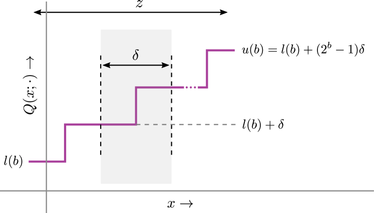
Figure 2: Schematic of the quantization operation of eq. (1)

.

A neural network is quantized by a set of $K$ quantizer $\{Q_{1},\ldots,Q_{K}\}$, each associated with a different part of the neural network, such as parameters or activations. In this paper, we assume symmetric uniform quantization [29] (i.e. $z=0$) for all quantizers in the network. Moreover, for quantizer $i$, the step-size $\delta_{i}$ is defined in terms of the quantizer bitwidth $b_{i}$ and a learned range parameter $\alpha_{i}$:

$$\delta_{i}=\frac{\alpha_{i}}{2^{b_{i}}-1}.$$ (2)

For ease of presentation, throughout this paper, we assume unsigned integer quantization. For more details on neural network quantization, we refer the reader to [29, 17].

To enable gradient-based learning during QAT, we need to overcome the fact that the gradient of the step function is zero almost everywhere. A common solution is to approximate the gradient of the quantization function w.r.t. its input with the straight-through estimator (STE) [21, 3]. [14, 25] extend this approach to allow for gradient-based range learning.

2.1 Pseudo-quantization noise

Quantization has been studied in-depth in classical signal processing literature [18]. A common assumption is that the quantization error $\epsilon=x-Q(x)$ is uniformly distributed with zero-mean and a standard deviation of $\delta/\sqrt{12}$, where $\delta$ denotes the step-size of the quantizer $Q$. This assumption can be shown to hold exactly under some conditions [44, 45]. The relationship between quantization noise and quantization is studied in-depth in [46] and, when used in practice, the noise $\epsilon_{q}=x-Q(x)\sim\mathcal{U}\left[-\frac{\delta}{2},\frac{\delta}{2}\right]$ is referred to as pseudo-quantization noise (PQN).

Following the PQN formulation, we define the pseudo-quantization noise quantizer $Q_{P}$ as follows:

$$Q_{P}(x;z,\delta,b)=\delta\cdot\mathrm{clamp}\left(\frac{x+z}{\delta}+\epsilon;l(b),u(b)\right)-z.$$ (3)

Here $\epsilon\sim\mathcal{[}-\frac{1}{2},\frac{1}{2}]$ and everything else remains the same as in (1). The PQN formulation is an attractive proposition for QAT because it is differentiable and, for this reason, it has been studied by [8, 38]. However, there is no concrete evidence that it outperforms hard quantization with STE.

2.2 Mixed-precision quantization objective

In mixed-precision quantization, we want to solve a multi-objective optimization problem, which involves maximising the task performance while minimizing resource requirements. Assuming a neural network with parameters $\boldsymbol{\Theta}$, we quantize each part of this network is quantized by a separate quantizer $Q_{i}\in\{Q_{1},\ldots,Q_{K}\}$. For example, one quantizer for parameters and activations per layer. Let $b_{i}\in\boldsymbol{b}=[b_{1},\ldots,b_{K}]$ denote the bitwidth associated with quantizer $Q_{i}$. We denote the quantized forward pass of this neural network, using a specific bitwidth allocation as $Q(\boldsymbol{\Theta},\boldsymbol{b})$ and the quantized task loss as $\mathcal{L}(Q(\boldsymbol{\Theta},\boldsymbol{b}))$ for an arbitrary task loss $\mathcal{L}$.

To complete the MPQ task, we introduce a resource cost $\pi(\boldsymbol{b})$, e.g., memory requirements, CPU cycle counts, or run-time. Throughout this paper, we assume the resource cost (or constraint) is either differentiable or a differentiable relaxation exists. An often used approach to MPQ task is minimizing a scalarized objective [41, 40, 38] similar to:

$$\mathcal{L}_{\textrm{MPQ}}(\boldsymbol{\Theta},\boldsymbol{b})=\lambda\mathcal{L}(Q(\boldsymbol{\Theta};\boldsymbol{b}))+\pi(\boldsymbol{b}),$$ (4)

where $\lambda>0$ is a scaling factor that weights the relative importance between the task loss and the resource cost. This approach is common because it allows us to learn the bitwidths and network parameters simultaneously, but it suffers from two main drawbacks: (1) it requires searching over values of $\lambda$ to find a trade-off that is acceptable to the user, and (2) there are no guarantees that the constraint will be met (cf. section 5.3). Our proposed method is designed to mitigate these constraints.

3 QBitOpt

We introduce QBitOpt, our novel method for mixed-precision quantization (MPQ). We previously established that the MPQ objective is a multi-objective optimization problem. As a result, the solution to the scalarized objective from equation (4) will depend on the weighting term $\lambda$. In practice, finding the optimal $\lambda$ between the two objectives that meet real-life resource constraints can be cumbersome and time-consuming. Instead, choosing a strict upper bound on the resources and optimizing the task performance within these bounds would be beneficial.

We adopt this approach for QBitOpt, resulting in the following constrained optimization objective:

minimize $$\mathcal{L}_{\textrm{Q}}(\boldsymbol{\Theta},\boldsymbol{b})=\mathcal{L}(Q(\boldsymbol{\Theta},\boldsymbol{b}))$$ (5)

subject to $$\widehat{\pi}(\boldsymbol{b})\preceq 0$$

In the above, $\widehat{\pi}(\cdot)$ denotes the resource constraint and $\preceq$ element-wise inequality. This encodes a similar resource cost as $\pi(\cdot)$ in equation (4). However, instead of minimizing the resource constraint, we only aim to satisfy an upper-bound constraint. Note that whereas we describe our method in terms of parameter quantization, this is not an intrinsic limitation of our method. We discuss details of activation quantization in appendix A.

Following the PQN model, we approximate the optimization objective further:

$$\mathcal{L}(Q_{P}(\boldsymbol{\Theta},\boldsymbol{b})) \approx\mathbb{E}_{\boldsymbol{\epsilon}}\left[\mathcal{L}(\boldsymbol{\Theta}+\boldsymbol{\epsilon}^{\prime})\right],\quad\boldsymbol{\epsilon}^{\prime}\sim\mathcal{U}[-\frac{\boldsymbol{\delta}}{2},\frac{\boldsymbol{\delta}}{2}],$$ (6)

$$=\mathbb{E}_{\boldsymbol{\epsilon}}\left[\mathcal{L}(\boldsymbol{\Theta}+\frac{\boldsymbol{\alpha}}{2^{b}-1}\boldsymbol{\epsilon})\right],\quad\boldsymbol{\epsilon}\sim\mathcal{U}[-\frac{1}{2},\frac{1}{2}],$$

where $\boldsymbol{\delta}=[\delta_{1},\ldots,\delta_{|\Theta|}]$ denotes the step-size associated with each parameter. Moreover, $\boldsymbol{\alpha}$ and $\boldsymbol{b}$ broadcast to the parameter dimensions. Following our formulation, the step size is a function of both the quantizer range $\boldsymbol{\alpha}$ and the bitwidth $\boldsymbol{b}$. The reparametrization in the second equality follows from this. By splitting the optimization objective in (5) over the network parameters and the bitwidth allocation into two separate minimizations, and substituting the result of equation (6), we obtain our QBitOpt optimization objective:

$$\min_{\boldsymbol{\Theta}}\min_{\boldsymbol{b}}\mathbb{E}_{\boldsymbol{\epsilon}}\left[\mathcal{L}\left(\boldsymbol{\Theta}+{\frac{\boldsymbol{\alpha}}{2^{\boldsymbol{b}}-1}}{\boldsymbol{\epsilon}}\right)\right]\quad\textrm{s.t. }\widehat{\pi}(\boldsymbol{b})\preceq 0.$$ (7)

This objective can now be optimized directly using, e.g., the penalty method [47] or the augmented Lagrangian method [47]. However, this would require retraining the neural network to converge multiple times, which is costly. Instead, in QBitOpt, we efficiently solve an approximation to the inner minimization problem and use the solution $\boldsymbol{b}^{\ast}$ to update $\boldsymbol{\Theta}$ using common gradient-based QAT techniques.

3.1 Approximate bitwidth minimization

The QBitOpt optimization, as stated in (7), can be solved directly, but doing so may be very costly. To enable gradient-based training of the network parameters $\boldsymbol{\Theta}$, we derive an efficient method for inferring the quantizer bitwidth and solving the bitwidth allocation problem. To this end, we focus on the inner optimization problem of (7), that is,

$$\boldsymbol{b}^{\ast}=\operatorname*{arg\,min}_{\boldsymbol{b}}\mathbb{E}_{\boldsymbol{\epsilon}}\left[\mathcal{L}\left(\boldsymbol{\Theta}+{\frac{\boldsymbol{\alpha}}{2^{\boldsymbol{b}}-1}}{\boldsymbol{\epsilon}}\right)\right]\quad\textrm{s.t. }\widehat{\pi}(\boldsymbol{b})\preceq 0.$$ (8)

We first approximate (8) using a second-order Taylor approximation w.r.t $\boldsymbol{\alpha}/(2^{\boldsymbol{b}}-1)$ around $\boldsymbol{0}$:

$$\boldsymbol{b}^{\ast}=\min_{\boldsymbol{b}}\boldsymbol{h}^{\top}\left(\frac{\boldsymbol{\alpha}}{2^{\boldsymbol{b}}-1}\right)^{2}, \boldsymbol{h}_{i}=\nabla^{2}\mathcal{L}(\boldsymbol{\Theta})_{ii}$$ (9)

$$\textrm{subject to }\widehat{\pi}(\boldsymbol{b})\preceq 0,$$

where $\boldsymbol{h}$ is the diagonal of the Hessian of the neural network. The first-order term cancels because the expectation of the pseudo-quantization noise is zero, and the constant term does not depend on $\boldsymbol{b}$. For the full derivation, see appendix B. The obtained objective is similar to the objective in [11]. However, they make an explicit assumption that the pre-trained floating-point network has converged, whereas we reach the same conclusion using only the zero-mean PQN assumption and make no assumptions about the state of the network. This distinction is important when solving (7) because it allows us to solve this inner optimization during QAT regardless of whether the outer optimization over $\boldsymbol{\Theta}$ has converged yet.

Depending on the exact choice of resource constraints $\widehat{\boldsymbol{\pi}}$, (9) is a convex program and can be solved very efficiently. In section 3.2, we discuss the choice of resource constraints and optimization methods in more detail.

Putting everything together, the QbitOpt optimization procedure consists of the following steps: first, solve (9) to obtain $\boldsymbol{b}^{\ast}$, and second, perform backpropagation keeping $\boldsymbol{b}^{\ast}$ constant to update step for $\boldsymbol{\Theta}$ and $\boldsymbol{\alpha}$ using gradients:

$$\nabla_{(\boldsymbol{\Theta},\boldsymbol{\alpha})}\mathbb{E}_{\boldsymbol{\epsilon}}\left[\mathcal{L}\left(\boldsymbol{\Theta}+\frac{\boldsymbol{\alpha}}{2^{\boldsymbol{b}^{\ast}}-1}\boldsymbol{\epsilon}\right)\right]$$ (10)

3.1.1 Quantization Sensitivities

The optimization procedure we established for $\boldsymbol{b}$ in (9) depends on the diagonal of the Hessian of the neural network. In this optimization problem, the Hessian diagonal captures how sensitive a parameter or a group of parameters is to quantization or perturbations in general. We formally define sensitivity as a statistic that quantifies how much the output of a neural network is affected by quantization. The diagonal of the Hessian in (9) is only one type of sensitivity, and one can imagine using other measures of sensitivity. In fact, this could be beneficial as calculating the Hessian diagonal of a neural network is often computationally expensive. This is why we use an approximation to the hessian diagonal called FIT [50]. Another potential shortcoming of the Hessian is that it captures the effect of infinitesimal perturbations, whereas low-bit quantization perturbations may be pretty significant. We leave such an investigation for future work.

FIT is a sensitivity that has been shown to correlate well with the hessian diagonal [50]. For this reason, we use FIT as a drop-in replacement for the more expensive hessian diagonal. It is defined as:

$$\widetilde{\boldsymbol{h}}_{i}=\left[\nabla_{\boldsymbol{\Theta}}\mathcal{L}(\boldsymbol{\Theta})\right]^{2}.$$ (11)

Note that FIT, similar to the hessian sensitivity, is computed based on the non-quantized neural network. As such, it requires an extra full precision forward and backward pass to compute and update sensitivities. Moreover, since we can only obtain gradients with respect to a subset of the training set, the computed FIT sensitivities are stochastic in nature. To address the stochasticity in the sensitivity estimation and to reduce the computational requirements, we keep a running exponential moving average of FIT sensitivities and only update them every $\tau$ iteration. See Section D.3 for more details on the choice of the EMA estimator.

So far, we have only focused on the quantization noise that stems from the rounding operator and can be effectively modeled as additive noise with PQN. However, the quantization operator of equation (1) also involves clipping of values outside the quantization grid limits. Clipping becomes an integral part of the training during QAT and can lead to considerable accuracy degradation if removed from the quantized model [1]. For this reason, we compute FIT using the clipped model parameters $\widetilde{\boldsymbol{\Theta}}=\textrm{clip}(\boldsymbol{\Theta},\boldsymbol{\alpha})$.

3.2 Choice of Resource Constraints and Optimization Methods

So far, we have left the resource constraint $\widehat{\pi}(\cdot)$ undefined. In this section, we discuss the choices for $\widehat{\pi}(\cdot)$ and its implications on the optimization problem. We aim to satisfy two goals: First, the optimization problem must be efficiently solved to be integrated into training, and second, the constraints should express realistic resource constraints. We accomplish the first goal by restricting the constraints to be of the form:

$$\widehat{\pi}_{i}(\boldsymbol{b}) \leq 0\quad i=1,\ldots,m$$ (12)

$$\rho_{j}(\boldsymbol{b}) =0\quad j=1,\ldots,p,$$ (13)

where the inequality constraint functions $\widehat{\pi}_{i}(\boldsymbol{b})$ are convex functions and the equality constraint functions $\rho_{i}(\boldsymbol{b})$ are affine. Combining constraints of this form with the optimization objective (9) results in a convex program [4]. Such convex programs can be solved efficiently using off-the-shelf convex optimization libraries, such as [9], allowing us to solve the bitwidth allocation problem frequently during training. In section 5.2, we demonstrate that updating bitwidths during training leads to higher task performance.

The convexity constraints of (12) and  (13) may appear quite restrictive at first, but a lot of real-life constraints can be expressed this way, such as the BOPs, the network’s average bitwidth or the network size bits. Even if the resource constraints are not strictly convex, there is extensive literature on expressing non-convex problems as convex optimization problems [4, Part II].

In our constraint optimization objective so far, we have not restricted the solution $\boldsymbol{b}^{\ast}$ to be a positive integer, which is necessary for finding realistic solutions. Including such a constraint turns the optimization problem into an integer program which is, in general, NP-complete [33] and would be infeasible to solve for large networks. However, certain resource constraints admit efficient and specific optimization procedures. For example, the average bitwidth constraint admits the greedy integer method presented in Algorithm 2. Alternatively, we can relax the integer constraint by allowing fractional bits and solve the optimization problem efficiently using a convex program. We can use this relaxation during the bitwidth update phase of training, where speed is important, and perform a final expensive integer program to infer the final bitwidth allocation before the final fine-tuning stage. We discuss these choices in more detail in ablation studies of section 5.2.

3.3 Integrated QBitOpt QAT pipeline

Algorithm 1 describes our integrated QAT and QBitOpt pipeline. At each training iteration, we update the quantization sensitivities $S_{q}$ for each quantizer using an exponential moving average, as described in (3.1.1), and perform a back-propagation step keeping the bitwidth $\boldsymbol{b}$ to update the network $\boldsymbol{\Theta}$ and quantization parameters $\boldsymbol{\alpha}$. For every $\tau$ iteration, we update the quantizer bitwidth, solving the convex optimization problem under the specified resource constraint, described in section 3.2. We do not update the bitwidths at every iteration in order to reduce the computational overhead and to give the network parameters enough time to adjust to the new bitwidth allocation. For a high-level schematic, see Figure 1.

Algorithm 1 QBitOpt

Neural network $\mathcal{N}$, task loss $\mathcal{L}(\cdot)$, resource constraints $\widehat{\pi}(\cdot)$, and sensitivity method $\mathcal{S}$

for iteration $i=1,\ldots,T$ do

     for quantizer $q=1,\ldots,K$ do

         $S^{(i)}_{q}=\gamma\mathcal{S}(\mathcal{L}(\boldsymbol{\Theta}^{(i-1)}))_{q}+(1-\gamma)S^{(i-1)}_{q}$

     end for

     if $i\textrm{ mod }\tau$ == 0 then

         $\boldsymbol{b}=\textrm{BitOptimizer}(S_{1}^{(i)},\ldots,S_{k}^{(i)})$

     end if

     $\boldsymbol{\Theta}^{(i)}=\boldsymbol{\Theta}^{(i-1)}+\eta\nabla_{\boldsymbol{\Theta}}\mathcal{L}(Q(\boldsymbol{\Theta}^{(i-1)};\boldsymbol{b},\boldsymbol{\alpha}^{(i-1}))$

     $\boldsymbol{\alpha}^{(i)}=\boldsymbol{\alpha}^{(i-1)}+\eta\nabla_{\boldsymbol{\alpha}}\mathcal{L}(Q(\boldsymbol{\Theta}^{(i-1)};\boldsymbol{b},\boldsymbol{\alpha}^{(i-1}))$

end for

Algorithm 2 Greedy integer assignment for average bitwidth

Initialize $\boldsymbol{b}\leftarrow[1,\ldots,1]$

$\mathcal{B}\leftarrow|\boldsymbol{b}|\cdot(\boldsymbol{\beta}-1)$

$\mathcal{S}_{q}\leftarrow$ sum of param./act. sensitivities for quantizer $q$

for iteration $1,\ldots,\mathcal{B}$ do

     $q\leftarrow\operatorname*{arg\,min}_{j}\mathcal{S}_{j}\left[\boldsymbol{\alpha}_{j}/(2^{\boldsymbol{b}_{j}}-1)\right]$

     $\boldsymbol{b}_{q}\leftarrow\boldsymbol{b}_{q}+1$

end for

4 Related Work

Neural network quantization has been a topic of interest in the research community for several years due to attractive hardware properties of quantized networks [7, 19, 24, 2, 14]. For recent in-depth surveys on PTQ and QAT topics, we refer the reader to [29] and [17].

Several methods for MPQ have been introduced in recent years. In gradient-based MPQ approaches [41, 40, 20, 48], a bitwidth for each quantizer is learned through gradient-based optimization. An extension of gradient-based methods can be found in PQN-based approaches [8, 38]. Using PQN instead of simulated quantization avoids the (biased) STE [21] and allows direct learning of each quantizer’s bitwidth. While these methods are efficient to run, defining a specific resource or accuracy target is impossible. Instead, a search over some regularization hyper-parameter is necessary. Several reinforcement learning techniques have been introduced [42, 35], in which an agent selects quantization policies that balance hardware constraints with accuracy targets. These methods show promising results but require very long training times to achieve good performance.

Our work extends to a different branch of MPQ literature, in which sensitivity is used as a statistic to select a bitwidth for each quantizer. In these methods, quantizers with high quantization sensitivity are assigned higher bitwidths. Similarly to our work, the HAWQ line of research [11, 10, 49] defines sensitivity as either the spectral norm or the trace of the Hessian. Their approach significantly differs from ours in how sensitivity is incorporated: due to the large computational requirements of their method, bitwidths are only estimated once, after which the network is iteratively fine-tuned. [51] use a first-order Taylor expansion information to estimate sensitivity during QAT and reduce bitwidths for quantizers for the least sensitive quantizers. Since their method only allows iterative bitwidth reduction, it can never recover from faulty bitwidth assignments. Taking a slightly different approach, [32] measure a quantizer’s sensitivity through signal-to-noise ratio on the network’s output by lowering the bitwidth of a target quantizer. They then use this information to iteratively reduce each quantizer’s bitwidth until some target accuracy or efficiency metric is reached. While the authors show good results, similarly to the HAWQ line of work, this approach is too slow to incorporate in QAT and is only used in PTQ settings. FIT [50] proposes a new sensitivity metric based on the trace of the Empirical Fisher matrix, which efficiently approximates the computationally expensive Hessian sensitivity in HAWQ. We use this sensitivity metric in QBitOpt to perform bitwidth allocation during QAT efficiently. Lastly, [37] compares several sensitivity metrics for post-training MPQ.

5 Experiments

In this section, we evaluate the effectiveness of QBitOpt by comparing it with other fixed-precision QAT methods and mixed-precision methods from the literature on the ImageNet [36] classification benchmark. We focus on low-bit quantization (4 and 3 bits on average) of efficient networks with depth-wise separable methods that are generally harder to quantize than fully convolutional networks [30, 29].

5.1 Experimental setup

Quantization

We follow the example of existing QAT literature and quantize the input to all layers except for the first layer and normalizing layers. In contrast to most existing QAT literature, we quantize all layers, including the first and last layer, and let QBitOpt decide the optimal bitwidth for these layers. We quantize weights (per-channel) and activation (per-tensor) using hard quantization and train all network parameters, including the quantization threshold $\alpha$, using the straight-through estimator, similar to LSQ  [14].

Mixed-Precision

Our training consists of two phases. In the first phase of mixed-precision QAT, we calculate FIT sensitivities while training the quantized network and re-allocate bitwidths every $\tau$=250 training iterations. In the second (or fine-tuning) phase, we freeze the obtained bitwidth allocation and fine-tune the remainder of the trainable parameters. This two-phase approach is quite common in the mixed-precision literature [38, 41]. Both phases are balanced in our experiments, and each takes up 50% of the training time unless stated otherwise. We study the effect of this choice in table 4.

Resource Constraint

In most experiments, we use the average bitwidth constraint across all quantizers in the neural network, including activations and weights. We restrict the bitwidths to integers that are greater or equal to 2 bits and solve the optimization problem with the greedy algorithm 1. The abbreviation $X$/$X$${}_{\text{MP}}$ below reflects this constraint with a target average bitwidth of $X$.

In table 6, we additionally use the per-element average bitwidth constraint, which is applied independently for weights and activations:

$$\rho_{w}(\boldsymbol{b}_{w}) =\frac{\sum_{i}b_{i}^{w}\cdot e_{i}^{w}}{\sum_{i}e_{i}^{w}},\quad\boldsymbol{b}_{w}\preceq 2,$$ (14)

$$\rho_{a}(\boldsymbol{b}_{a}) =\frac{\sum_{i}b_{i}^{a}\cdot e_{i}^{a}}{\sum_{i}e_{i}^{a}},\quad\boldsymbol{b}_{a}\preceq 2,$$ (15)

where $b_{i}^{w}$/$b_{i}^{a}$ and $e_{i}^{w}$/$e_{i}^{a}$ denote the bitwidth and number of elements of the $i$^th layer’s weight/activation, respectively. We include these results for a fair comparison to the NIPQ [38] method, which uses this constraint.

Optimization

In all cases, we start from a pre-trained full-precision network (see appendix C.3 for the origin of the checkpoints) and instantiate the weight and activation quantization parameters using MSE range estimation [29]. We train MobileNetV2 and EfficientNet-Lite for 30 epochs with SGD and momentum of 0.9 and MobileNetV3-Small for 40 epochs. More details about the optimization can be found in the appendix C.1.

5.2 Ablation studies

As we discussed in section 2, our QBitOpt framework can be easily combined with existing QAT methods and deal with fractional or integers bitwidths thanks to its speed and flexibility. In this section, we explore how different quantization and optimization options influence the performance of our framework.

Sensitivities computation

Architecture	W/A	$\widetilde{\boldsymbol{h}}$FP	$\widetilde{\boldsymbol{h}}$clip
MobileNetV2	4/4${}_{\text{MP}}$	69.44	69.71
MobileNetV3-Small	4/4${}_{\text{MP}}$	63.47	64.23
	3/3${}_{\text{MP}}$	56.64	57.14

Table 1: QBitOpt using clipped sensitivities $\widetilde{\boldsymbol{h}}$_clip and full-precision sensitivities $\widetilde{\boldsymbol{h}}$_FP. Validation accuracy (%) on ImageNet.

In section 3.1.1, we argued that clipped network sensitivities are better suited for inferring bitwidth during QAT, compared to vanilla full-precision sensitivities, as PQN models the noise from the rounding operator but not any clipping. The results in table 1 confirm our hypothesis and show that in all cases, using the clipped sensitivities leads to better accuracy. In some cases, such as for MobileNetV3, not clipping during sensitivity computation can result in a substantial accuracy drop.

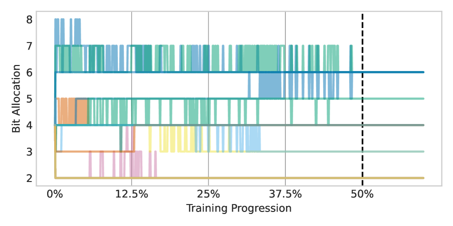
(a) Bit allocation using greedy integer bit optimization

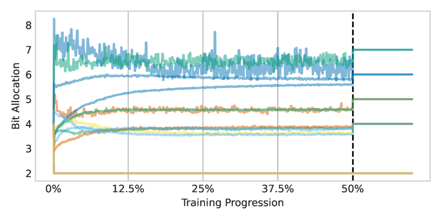
(b) Bit allocation using fractional bit optimization

Figure 3: Bit allocation during training is reasonably stable, i.e., there are changes over time, but no sudden changes

Fractional vs. integer bitwidth

Architecture	W/A	Fractional	Integer
MobileNetV2	4/4${}_{\text{MP}}$	67.91	69.71
	3/3${}_{\text{MP}}$	65.65	65.65
MobileNetV3-Small	4/4${}_{\text{MP}}$	64.23	64.39
	3/3${}_{\text{MP}}$	57.14	57.14

Table 2: QBitOpt optimization method: integer vs. fractional bits. Validation accuracy (%) on ImageNet.

In section 3.2, we discussed that constraining all bitwidths to natural numbers turns the convex program into an integer program, which is NP-hard. Here, we experimentally validate and compare our two proposed solutions, the greedy integer method and fractional bitwidth. In table 2, we show the effect of both optimization methods on the final accuracy. We observe that in most cases, these lead to very similar performance, and there is no clear winner, except for MobileNetV2 with a 4 bits target where greedy integers perform better. In figure 3, we illustrate the progression of the bitwidth allocation during training. We observe that for greedy integer (cf. 3(a)), some bitwidths oscillate between two values which could introduce noise in the network optimization. On the other hand, fractional bitwidths (cf. 3(b) progress much smoother during mixed precision phase, however at the end of the phase, there is a jump once the bitwidth gets rounded to a viable natural number for the fine-tuning phase. For the remainder of the experiments, we favor greedy integers over fractional bitwidths.

Pseudo-noise vs. hard quantization

Architecture	W/A	Hard Quant	PQN
MobileNetV2	4/4${}_{\text{MP}}$	69.71	69.25
	3/3${}_{\text{MP}}$	65.65	64.21
MobileNetV3-Small	4/4${}_{\text{MP}}$	64.23	53.92
	3/3${}_{\text{MP}}$	57.14	14.61

Table 3: Comparison of training with hard quantization and STE compared to PQN for the mixed-precision phase of QAT. Validation accuracy (%) on ImageNet.

In the mixed precision phase, we jointly train the network weights leveraging QAT while updating the bitwidth allocation. Since updating the sensitivities is independent of the QAT update, we can choose any quantization method for QAT. Two natural choices are pseudo-quantization noise (PQN), which we used to derive our sensitivity metric, and hard-quantization with STE, which is commonly used in most QAT literature [24, 26, 14, 30]. In table 3, we experimentally compare both choices. Hard quantization with STE outperforms PQN for all models tested. Particularly for MobileNetV3-Small, the performance gap between the methods is quite significant. We hypothesize that it is important for the network to early in training adapt to the exact quantization noise present during inference.

Two-phase mixed-precision training

Arch.	W/A	0%	25%	50%	75%	100%
MNv2	4/4${}_{\text{MP}}$	68.63	69.55	69.71	69.7	67.81
	3/3${}_{\text{MP}}$	62.71	65.83	65.65	65.56	62.47
MNv3	4/4${}_{\text{MP}}$	59.62	64.39	64.23	64.34	62.66
	3/3${}_{\text{MP}}$	43.70	57.49	57.14	56.9	54.94

Table 4: Comparing training MobileNetV2 (MNv2) and MobileNetV3-Small (MNv3) with QBitOpt for different fractions (%) of the total training time. 0% corresponds to using QBitOpt on a subset of training data to allocate bitwidths and freezing that allocation during training. Validation accuracy (%) on ImageNet.

In this section, we study the impact of our two-phased mixed-precision training. In table 4, we show the results with various divisions of the training time between the mixed precision phase and the fine-tuning phase. Most importantly, these results demonstrate that both phases are important for obtaining the best mixed-precision performance. When only fine-tuning is used after a post-training bitwidth allocation (0% column), the performance significantly degrades compared to updating the bitwidth during training using QBitOpt — especially for 3-bit quantization. This shows that our novel QBitOps algorithm, which integrates bitwidth allocation into QAT, compares favorably to common post-training MPQ followed by fine-tuning. On the other hand, updating the bitwidth allocations up to the conclusion of training (100% column) adversely affects performance. The non-constant bitwidths add extra noise to the optimization procedure. This can be harmful in the last phase of training, as discussed in the previous paragraph, and is a common issue known in the MPQ literature. As such, most training-based approaches circumvent this by not updating the bitwidths towards the end of training [41, 38].

While having both phases is clearly essential in finding the best mixed-precision network, our framework is relatively stable to the exact division of the training time between them. For most networks and bitwidth, using between 25% and 75% for the mixed precision phase leads to good results.

5.3 Comparison to existing methods

	Method	W/A	Avg. Bits	Acc. (%)
MobileNetV2	Full-precision	32/32	-	71.72
	LSQ [14]	4/4	4.0	69.450.07
	DQ [40]	4/4${}_{\text{MP}}$	4.080.01	68.550.30
	NIPQ [38]	4/4${}_{\text{MP}}$	4.110.0	69.130.07
	QBitOpt (ours)	4/4${}_{\text{MP}}$	4.0	69.750.04
	LSQ [14]	3/3	3.0	65.170.12
	DQ [40]	3/3${}_{\text{MP}}$	3.100.01	64.860.07
	NIPQ [38]†	3/3${}_{\text{MP}}$	3.150.0	62.250.5
	QBitOpt (ours)	3/3${}_{\text{MP}}$	3.0	65.710.07
MobileNetV3-Small	Full-precision	32/32	-	67.67
	LSQ [14]	4/4	4.0	61.580.07
	DQ [40]	4/4${}_{\text{MP}}$	4.100.01	63.600.02
	NIPQ [38]	4/4${}_{\text{MP}}$	4.110.01	62.210.15
	QBitOpt (ours)	4/4${}_{\text{MP}}$	4.0	64.340.06
	LSQ [14]	3/3	3.0	51.920.04
	DQ [40]	3/3${}_{\text{MP}}$	3.090.01	57.260.44
	NIPQ [38] †	3/3${}_{\text{MP}}$	3.220.01	56.250.72
	QBitOpt (ours)	3/3${}_{\text{MP}}$	3.0	57.360.17
EfficientNet-lite	Full-precision	32/32	-	75.42
	LSQ [14]	4/4	4.0	72.930.09
	DQ [40]	4/4${}_{\text{MP}}$	4.080.01	72.290.21
	NIPQ [38]	4/4${}_{\text{MP}}$	4.100.01	72.270.05
	QBitOpt (ours)	4/4${}_{\text{MP}}$	4.0	73.320.10
	LSQ [14]	3/3	3.0	69.620.15
	DQ [40]	3/3${}_{\text{MP}}$	3.130.01	68.820.21
	NIPQ [38]	3/3${}_{\text{MP}}$	3.130.01	66.560.12
	QBitOpt (ours)	3/3${}_{\text{MP}}$	3.0	70.000.07

Table 5: Comparison of QBitOpt with other methods on the ImageNet image classification benchmark. We report validation accuracy (%), target bitwidth (W/A) set for the corresponding method and the achieved average bitwidth (Avg. Bits) for mixed-precision methods. We run 3 seeds for all experiments and report the mean result and STD in the superscript.^† only 2 seeds available due to unstable training.

	Method	Bits(W/A)	Acc. (%)
MNv2	NIPQ	4.080.0/4.090.03	70.700.02
	QBitOpt (ours)	4/4	70.390.05
	NIPQ	3.10.0/ 3.080.02	67.060.28
	QBitOpt (ours)	3/3	68.440.0
MNv3-Small	NIPQ	4.2090.06/4.1540.06	61.011.64
	QBitOpt (ours)	4/4	62.450.21
	NIPQ	-	-
	QBitOpt (ours)	3/3	57.820.29
EffNet	NIPQ†	4.0650.0/ 4.1190.00	73.620.03
	QBitOpt (ours)	4/4	73.010.11
	NIPQ	3.0660.03/ 3.0890.01	70.700.14
	QBitOpt (ours)	3/3	72.130.08

Table 6: Comparison of QBitOpt and NIPQ [38] for the per-element average bitwidth objective independently optimized for weights and activation. We report validation accuracy (%) and the achieved per-element average bitwidth for weights and activations. We run 3 seeds for all experiments and report the mean result and STD in the superscript.^† no results available due to unstable training.

We compare QbitOpt to other QAT approaches: (a) LSQ [14] for fixed-precision quantization; (b) differentiable quantization (DQ) [40] and noise injection pseudo quantization (NIPQ) [38] for mixed-precision. For a fair comparison, we have re-implemented DQ and NIPQ, adhering to their implementation details and modifying them appropriately to match our constraints and quantization assumptions. We performed an extensive hyperparameter search on the regularization strength $\lambda$ and learning rates. For further details, refer to appendix D.

In table 5, we present the results for MobileNetV2, MobileNetV3-Small and EfficientNet-Lite on the ImageNet classification benchmark. QbitOpt significantly outperforms the strong fixed-precision LSQ baseline in all cases. Especially for the challenging to quantize MobileNetV3-Small, the accuracy improves up to 5%. We also outperform the mixed-precision method, NIPQ & DQ, in terms of quantized accuracy, even though NIPQ and DQ achieve a higher average bitwidth. These results showcase one of the biggest strengths of our method, namely that the resource constraint is met exactly. This contrasts with the other mixed-precision methods, where we struggle to meet the target constraint even after an extensive hyperparameter search.

In table 5, we compare QBitpt to NIPQ using the per-element average bitwidth implemented in their work (cf. equations (14) & (15)) for a fairer comparison. Under this less stringent constraint, the accuracy gap between the two methods closes, and in two cases, MobileNetV2 W4A4 and EfficientNet-Lite W4A4, NIPQ outperforms QBitOpt. However, the trend is reversed for 3 bits and, specifically, for MobileNetV3-Small training was unstable, and we could not reach satisfactory accuracy. Despite closing the accuracy margin, QBitOpt is the only method guaranteeing the resource constraint is met in all cases without searching for regularization strength, thus, significantly reducing experimentation time.

6 Conclusion

In this work, we introduced QBitOpt, a novel algorithm for allocating bitwidths under strict resource constraints. QBitOpt leverages techniques from convex optimization and QAT to obtain high-performing neural networks in the sense of resource requirements and task performance without the need to carefully balance task loss and resource cost through a cumbersome hyper-parameter. We justify using Hessian-based sensitivities, traditionally only used for fully converged neural networks, during training. Our greedy integer method and efficient FIT approximation allow us to regularly update the bitwidth allocations during quantization-aware training.

We demonstrate the efficacy of QBitOpt on several architectures in which QBitOpt compares favorably to competing fixed-precision and mixed-precision approaches. We further examine various properties of our method through ablation studies. Specifically, we show that regularly reallocating bitwidths during training is crucial for optimal performance. We identify improved sensitivities that more closely capture quantization perturbation and the design of convex relaxations for hardware constraints as exciting avenues for future research.

Appendix A Activation quantization

In section 2, we formulated the QBitOpt optimization objective in terms of network parameters $\boldsymbol{\Theta}$. However, we commonly also quantize the activations in neural network quantization. Fortunately, our method extends easily to activations too, as it is trivial to compute quantization sensitivities for activations. As a reminder, in section 3.1, we defined the Hessian diagonal $\boldsymbol{h}$ as an example of quantization sensitivity. By computing the hessian sensitivities with respect to activations, we can infer bitwidth allocation for activation as per equation 9.

Considering an arbitrary neural network $F$ with $L$ layers as a composition of functions:

$$F(\boldsymbol{x})=\left[f_{L}\circ f_{L-1}\circ\cdots\circ f_{2}\circ f_{1}\right](\boldsymbol{x}),$$ (16)

we can compute the sensitivity of the $i$^th activation $\boldsymbol{z}_{i}=\left[f_{i}\circ\cdots\circ f_{1}\right](\boldsymbol{x})$ by simply considering the sub-network:

$$F_{i+1}=\left[f_{L}\circ f_{L-1}\circ\cdots\circ f_{i+1}\right]$$ (17)

The hessian sensitivity is now given by:

$$\mathbb{E}_{\boldsymbol{x}\sim\mathcal{D}}\left[\frac{\partial^{2}}{\partial\boldsymbol{z}_{i}^{2}}\mathcal{L}\left(F_{i+1}(\boldsymbol{z})\right)\biggr{\rvert}_{\boldsymbol{z}=\boldsymbol{z}_{i}}\right]$$ (18)

The sensitivity can be computed over the full dataset $\mathcal{D}$ using an exponential moving average, as described in section 3.1.1. In practice, one may consider applying separate constraints to the parameter and activation quantizer bitwidth. We leave this investigation for future work.

Appendix B Inner bitwidth minimization

For convenience, we restate (7) here:

$$\min_{\boldsymbol{\Theta}}\min_{\boldsymbol{b}}\mathbb{E}_{\boldsymbol{\epsilon}}\left[\mathcal{L}\left(\boldsymbol{\Theta}+{\frac{\boldsymbol{\alpha}}{2^{\boldsymbol{b}}-1}}{\boldsymbol{\epsilon}}\right)\right]\quad\textrm{s.t. }\widehat{\pi}(\boldsymbol{b})\preceq 0.$$ (19)

As presented in the main text(cf. section 3.1), we aim to solve an approximation to the inner minimization. The solution to this is then used to take a gradient step for the outer minimization. First, let $\boldsymbol{\delta}=\boldsymbol{\alpha}/(2^{\boldsymbol{b}}-1)$. Then we approximate the objective using a second-order Taylor approximation:

$$\mathbb{E}_{\boldsymbol{\epsilon}}\left[\mathcal{L}(\boldsymbol{\Theta}+\boldsymbol{\delta}\boldsymbol{\epsilon})\right]$$ (20)

$$\approx\mathbb{E}_{\boldsymbol{\epsilon}}\left[\mathcal{L}(\boldsymbol{\Theta})+(\boldsymbol{\delta}\boldsymbol{\epsilon})^{\top}\nabla_{\boldsymbol{\Theta}}\mathcal{L}(\boldsymbol{\Theta})+\frac{1}{2}(\boldsymbol{\delta}\boldsymbol{\epsilon})^{\top}\nabla^{2}_{\boldsymbol{\Theta}}\mathcal{L}(\boldsymbol{\Theta})(\boldsymbol{\delta}\boldsymbol{\epsilon})\right]$$

The first term is constant with respect to $\boldsymbol{b}$ and the second term equals zero as $\mathbb{E}_{\boldsymbol{\epsilon}}[\boldsymbol{\epsilon}]=0$. This leaves the following optimization objective:

$$\frac{1}{2}\mathbb{E}_{\boldsymbol{\epsilon}}\left[(\boldsymbol{\delta}\boldsymbol{\epsilon})^{\top}\left[\nabla^{2}\mathcal{L}(\boldsymbol{\Theta})\right](\boldsymbol{\delta}\boldsymbol{\epsilon})\right]$$ (21)

$$\ \ =\frac{1}{2}\mathrm{Tr}\left\{\mathbb{E}_{\boldsymbol{\epsilon}}[(\boldsymbol{\delta}\boldsymbol{\epsilon})^{\top}\left[\nabla^{2}\mathcal{L}(\boldsymbol{\Theta})\right](\boldsymbol{\delta}\boldsymbol{\epsilon})\right]\}$$

$$\ \ \stackrel{{\scriptstyle(a)}}{{=}}\frac{1}{2}\mathrm{Tr}\left\{\mathbb{E}_{\boldsymbol{\epsilon}}[(\boldsymbol{\delta}\boldsymbol{\epsilon})(\boldsymbol{\delta}\boldsymbol{\epsilon})^{\top}\right]\left[\nabla^{2}\mathcal{L}(\boldsymbol{\Theta})\right]\}$$

$$\ \ =\frac{1}{2}\mathrm{Tr}\left\{\textrm{diag}(\boldsymbol{\delta})\mathbb{E}_{\boldsymbol{\epsilon}}[\boldsymbol{\epsilon}\boldsymbol{\epsilon}^{\top}\right]\textrm{diag}(\boldsymbol{\delta})\left[\nabla^{2}\mathcal{L}(\boldsymbol{\Theta})\right]\}$$

$$\ \ \stackrel{{\scriptstyle(b)}}{{=}}\frac{1}{24}\mathrm{Tr}\left\{\textrm{diag}(\boldsymbol{\delta})\textrm{diag}(\boldsymbol{\delta})\left[\nabla^{2}\mathcal{L}(\boldsymbol{\Theta})\right]\right\}$$

$$\ \ =\frac{1}{24}\mathrm{Tr}\left\{\textrm{diag}(\boldsymbol{\delta})^{2}\left[\nabla^{2}\mathcal{L}(\boldsymbol{\Theta})\right]\right\}$$

$$\ \ =\frac{1}{24}\sum_{i}^{|\boldsymbol{\Theta}|}\left[\nabla^{2}\mathcal{L}(\boldsymbol{\Theta})\right]_{ii}\boldsymbol{\delta}^{2}_{ii}.$$

Here, $(a)$ uses $\mathrm{Tr}(A^{\top}B)=\mathrm{Tr}(BA^{\top})$ where $A$ and $B$ are two $m\times n$ real matrices and $(b)$ follows from $\mathbb{E}[\boldsymbol{\epsilon}\boldsymbol{\epsilon}^{\top}]=\boldsymbol{I}/12$. Finally, dropping the multiplicative constants that do not affect the minimization problem and re-substituting $\boldsymbol{\delta}$, we obtain our optimization problem:

$$\boldsymbol{b}^{\ast}=\min_{\boldsymbol{b}}\boldsymbol{h}^{\top}\left(\frac{\boldsymbol{\alpha}}{2^{\boldsymbol{b}}-1}\right)^{2}, \boldsymbol{h}_{i}=\nabla^{2}\mathcal{L}(\boldsymbol{\Theta})_{ii}$$ (22)

$$\textrm{subject to }\widehat{\pi}(\boldsymbol{b})\preceq 0.$$

Appendix C Experimental configuration

Model	W/A	Epochs		SGD - Model parameters				Adam - Quant. parameters
		Phase-1	Phase-2	LR	$\eta_{min}$	Warmup	WD	LR	WD
MobileNetV2	4/4	15	15	0.0033	3.3$\times 10^{-6}$	-	1.0$\times 10^{-5}$	1.0$\times 10^{-5}$	$0.0$
	3/3	15	15	0.01	1.0$\times 10^{-5}$	-	1.0$\times 10^{-5}$	1.0$\times 10^{-5}$	$0.0$
EfficientNet-	4/4	15	15	0.0033	3.3$\times 10^{-6}$	-	1.0$\times 10^{-5}$	1.0$\times 10^{-5}$	$0.0$
Lite	3/3	15	15	0.01	1.0$\times 10^{-5}$	-	1.0$\times 10^{-5}$	1.0$\times 10^{-5}$	$0.0$
MobileNetV3-	4/4	20	20	0.07	7.0$\times 10^{-5}$	4	1.0$\times 10^{-5}$	1.0$\times 10^{-5}$	$0.0$
Small	3/3	20	20	0.05	5.0$\times 10^{-5}$	4	0.0	1.0$\times 10^{-5}$	$0.0$

Table 7: Optimization configuration: all model parameters (except for the quantization parameters) are optimized using SGD with a momentum of 0.9 and a cosine annealing schedule for learning rate. We use a separate Adam optimizer with a constant learning rate for the quantization parameters. WD: weight decay; Warmup: number of epoch for linear learning rate warmup; $\eta_{min}$: final learning rate of cosine decay.

C.1 Optimization

All experiments are trained on NVIDIA GPUs using Python 3.8.10, PyTorch v1.11, and Torchvision v0.12. We found that using separate optimizers for the model (SGD) and quantization parameters (Adam) leads to stabler training and higher accuracy across architectures and methods. The optimizer and learning rate schedules for both optimizers can be found in table 7. Phase-1 refers to QAT with bitwidth reallocation using QBitOpt, whereas in phase-2, we fix the quantizers’ bitwidth and fine-tune with QAT. At the end of each training epoch, we re-estimate the batch-normalization statistics using 50 batches of training data, as per [30].

C.2 QBitOpt configuration

During phase-1 of training, we calculate an exponential-moving average of each quantizer’s FIT sensitivity $S_{q}$ with a momentum of 0.9, as shown in algorithm 1. Because sensitivities change quite smoothly during training (see fig. 4), we decided to compute them only every two training iterations to reduce training time. We infer a new bitwidth allocation by solving the optimization every $\tau=250$ training iterations. We found that QBitOpt is not very sensitive to this hyperparameter, and decreasing $\tau$ did not lead to better results. In fact, given that we learn the quantization range $\alpha$ using gradients, $\tau$ should be large enough to allow the quantization range to adapt to the latest bitwidth allocation.

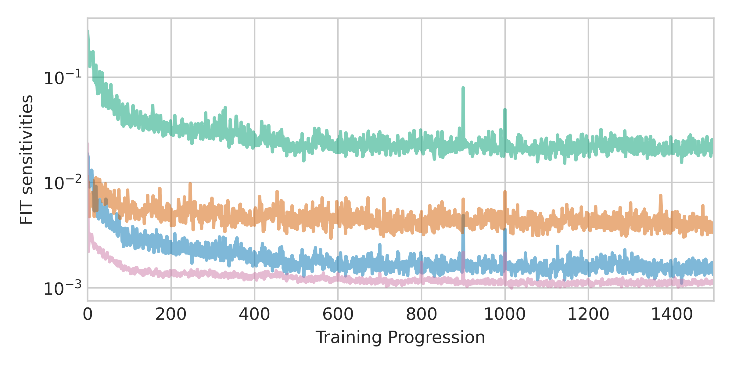
Figure 4: FIT sensitivities progression over time (y-axis in logarithmic scale)

C.3 Model checkpoints

• MobileNetV2: https://github.com/tonylins/pytorch-mobilenet-v2

• MobileNetV3-Small: https://pytorch.org/vision/0.12/models

• EfficientNet-Lite: https://github.com/huggingface/pytorch-image-models

Appendix D Additional experimental results

D.1 Differential quantization (DQ)

Method	Avg. bits	Acc. (%)
DQ [$\lambda=0.3$]	4.299	64.38
DQ [$\lambda=0.5$]	4.187	63.87
DQ [$\lambda=0.7$]	4.150	63.92
DQ [$\lambda=1.0$]	4.093	63.61
DQ [$\lambda=1.4$]	4.065	63.56
DQ [$\lambda=2.0$]	4.065	63.42
DQ [$\lambda=3.0$]	4.037	63.44
DQ [$\lambda=5.0$]	4.028	63.44
DQ [$\lambda=8.0$]	4.009	63.27
QBitOpt	4.0	64.23
DQ [$\lambda=0.3$]	3.542	60.45
DQ [$\lambda=0.5$]	3.402	59.62
DQ [$\lambda=0.7$]	3.290	58.48
DQ [$\lambda=1.0$]	3.215	58.33
DQ [$\lambda=1.4$]	3.159	57.95
DQ [$\lambda=2.0$]	3.121	57.63
DQ [$\lambda=3.0$]	3.084	56.86
DQ [$\lambda=5.0$]	3.056	55.70
DQ [$\lambda=8.0$]	3.037	56.89
QBitOpt	3.0	57.14

Table 8: MobileNetV3-Small on ImaneNet. DQ [40] results for different regularization strength $\lambda$, including our QBitOpt result. The values in bold are used in table 5.

Method	Avg. bits	Acc. (%)
DQ [$\lambda=0.3$]	4.210	69.09
DQ [$\lambda=0.5$]	4.143	68.59
DQ [$\lambda=0.7$]	4.105	68.57
DQ [$\lambda=1.0$]	4.076	68.50
DQ [$\lambda=1.4$]	4.067	68.51
DQ [$\lambda=2.0$]	4.038	68.80
QBitOpt	4.0	69.71
DQ [$\lambda=0.3$]	3.286	66.33
DQ [$\lambda=0.5$]	3.229	65.44
DQ [$\lambda=0.7$]	3.124	64.78
DQ [$\lambda=1.0$]	3.114	64.94
DQ [$\lambda=1.4$]	3.086	64.27
DQ [$\lambda=2.0$]	3.048	64.18
QBitOpt	3.0	65.65

Table 9: MobileNetV2 on ImaneNet. DQ [40] results for different regularization strength $\lambda$, including our QBitOpt result. The values in bold are used in table 5.

Method	Avg. bits	Acc. (%)
DQ [$\lambda=0.3$]	4.242	72.48
DQ [$\lambda=0.5$]	4.141	72.61
DQ [$\lambda=0.7$]	4.111	72.50
DQ [$\lambda=1.0$]	4.081	72.14
DQ [$\lambda=1.4$]	4.061	72.16
DQ [$\lambda=2.0$]	4.051	72.20
QBitOpt	4.0	73.43
DQ [$\lambda=0.3$]	3.354	70.03
DQ [$\lambda=0.5$]	3.212	69.24
DQ [$\lambda=0.7$]	3.141	68.95
DQ [$\lambda=1.0$]	3.121	68.86
DQ [$\lambda=1.4$]	3.101	68.48
DQ [$\lambda=2.0$]	3.051	68.33
QBitOpt	3.0	70.04

Table 10: EfficientNet-Lite on ImaneNet. DQ [40] results for different regularization strength $\lambda$, including our QBitOpt result. The values in bold are used in table 5.

In tables 9, 8 & 10, we present the results of our hyperparameter search over the regularization strength $\lambda$ in the objective of differential quantization (DQ) [40]. In contrast to QBitOpt, the method fails to reach the target average bitwidth exactly. Notably, for MobileNetV3-Small, we have to extend the grid search significantly to achieve a satisfactory average bitwidth solution. This study demonstrates the power of QBitOpt that does not really on a scalarized multi-objective loss. Instead, QBitOpt guarantees the exact constraint, enabling the user to focus on tuning the QAT hyperparameters and achieve the highest task performance under the specified constraint. Please note that the results in bold are shown in the final results table 5.

D.2 Noise injection pseudo quantization (NIPQ)

Method	Avg. bits	Acc. (%)
NIPQ [$\lambda=2.0$]	4.229	69.39
NIPQ [$\lambda=4.0$]	4.162	69.17
NIPQ [$\lambda=5.0$]	4.140	69.16
NIPQ [$\lambda=8.0$]	4.108	69.13
NIPQ [$\lambda=9.0$]	4.111	69.16
QBitOpt	4.0	69.71
NIPQ [$\lambda=3.0$]
NIPQ [$\lambda=4.0$]
NIPQ [$\lambda=5.0$]
NIPQ [$\lambda=7.0$]
NIPQ [$\lambda=9.0$]
NIPQ [$\lambda=10.0$]
QBitOpt	3.0	65.65

Table 11: MobileNetV2 on ImaneNet. NIPQ [38] results for different regularization strength $\lambda$, including our QBitOpt result. The values in bold are used in table 5.

Method	Avg. bits	Acc. (%)
NIPQ [$\lambda=3.0$]	4.192	72.49
NIPQ [$\lambda=4.0$]	4.182	72.52
NIPQ [$\lambda=6.0$]	4.131	72.38
NIPQ [$\lambda=7.0$]	4.125	72.37
NIPQ [$\lambda=9.0$]	4.104	72.32
NIPQ [$\lambda=10.0$]	4.104	72.29
NIPQ [$\lambda=11.0$]	4.101	72.29
QBitOpt	4.0	73.43
NIPQ [$\lambda=3.0$]	3.283	68.49
NIPQ [$\lambda=4.0$]	3.242	68.27
NIPQ [$\lambda=6.0$]	3.182	67.77
NIPQ [$\lambda=7.0$]	3.162	67.69
NIPQ [$\lambda=10.0$]	3.131	66.69
NIPQ [$\lambda=12.0$]	3.128	66.56
QBitOpt	3.0	70.04

Table 12: EfficientNet-Lite on ImaneNet. NIPQ [38] results for different regularization strength $\lambda$, including our QBitOpt result. The values in bold are used in table 5.

In tables 11 and 12, we present the results of our hyperparameter search over the regularization strength $\lambda$ in the objective of noise injection pseudo quantization (NIPQ) [38]. Similar to DQ, we observe that we need an extensive grid search over the regularization parameter to find a satisfactory average bitwidth solution. In fact, for NIPQ, we needed significantly stronger regularization values for all models.

D.3 Effect of $\alpha$-factor in exponential moving average on sensitivity estimation

In Section 3.1.1, it was mentioned that an exponential moving average (EMA) is used to estimate sensitivities over multiple batches during training. Specifically, given the observed sensitivity $e_{t}$ at timestep $t$ and $\alpha\in(0,1]$, the EMA $\mathcal{E}_{t}$ is defined as:

$$\mathcal{E}_{t}=(1-\alpha)\mathcal{E}_{t-1}+\alpha e_{t},\quad\mathcal{E}_{1}=e_{1}.$$ (23)

The choice of $\alpha$ determines how much weight is put on past observations compared to new observations. E.g., when $\alpha=1$, only the latest observations are used. Figure 5 shows results for different architectures trained using various values for $\alpha\in\{0.05,0.25,0.5,0.75,0.9,1.0\}$. This shows that the choice of $\alpha$ is insignificant, and one could choose not to include the exponential moving average estimator. This result agrees with the progression of FIT estimates shown in Figure 4, where we showed that sensitivities are relatively stable during training. However, since this figure also shows several outliers, we use the EMA estimator for the results presented in the main text.

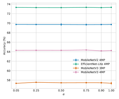
Figure 5: Accuracy obtained for different settings of $\alpha$ for the Exponential Moving Average sensitivity estimation. The whiskers, if visible, show the standard deviation over three seeds.

D.4 QBitOpt bitwidth allocation

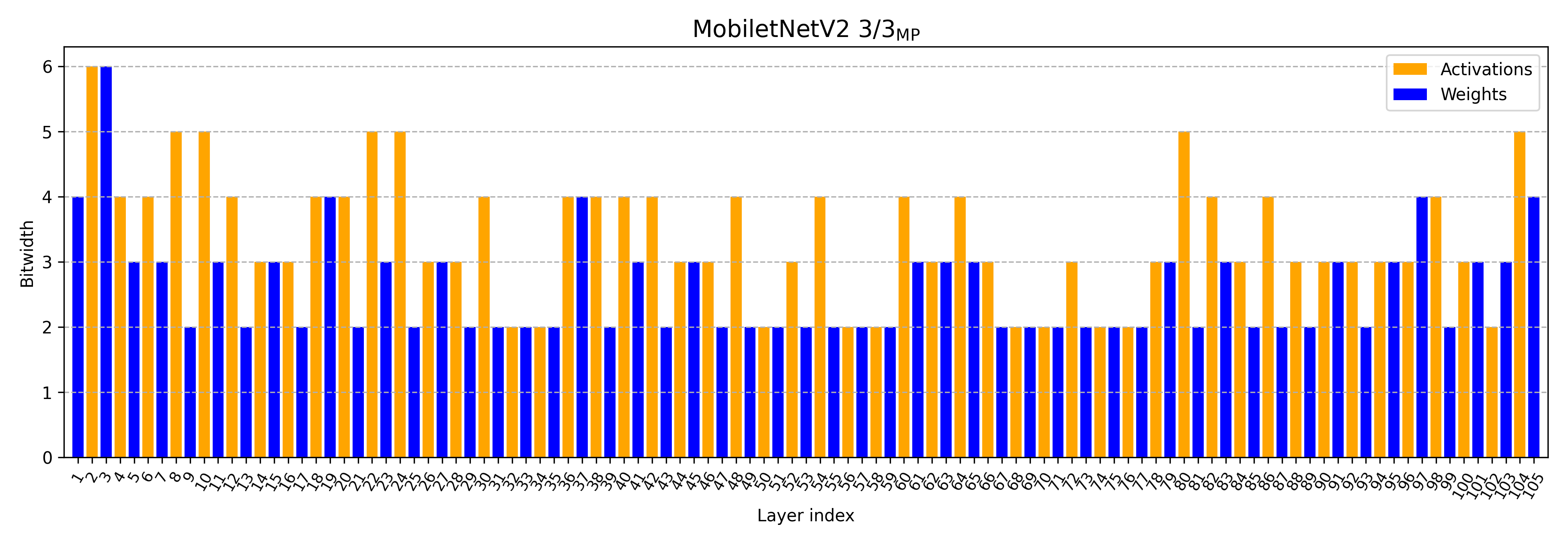
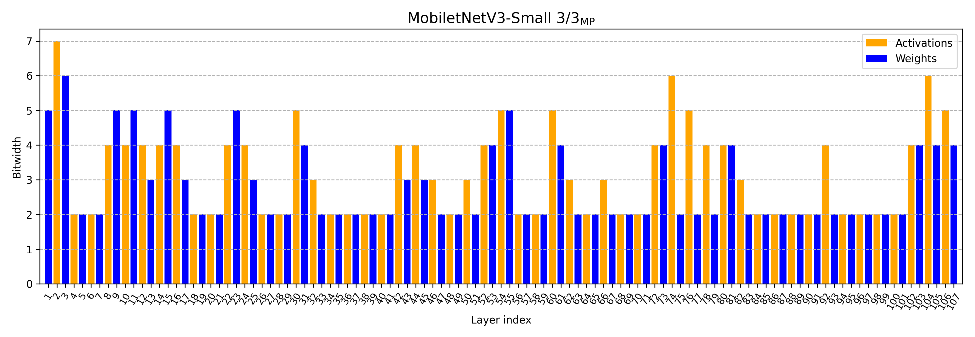
Figure 6: Final bitwidth allocation for MobileNetV2 and MobileNetV3-Small using QBitOpt with 3-bit average target bitwidth 3/3${}_{\text{MP}}$.

In figure 6, we illustrate the final bitwidth allocation resulting from QBitOpt on MobileNetV2 and MobileNetV3-Small with a 3-bit average target bitwidth. In both cases, QBitOpt allocated more bits in the first and last layers of the networks, which is consistent with empirical observations from existing literature. In addition, in MobileNetV2, we also observe that QbitOpt tends to assign higher bitwidth to activations compared to weights.

References

- [1] Milad Alizadeh, Arash Behboodi, Mart van Baalen, Christos Louizos, Tijmen Blankevoort, and Max Welling. Gradient l-1 regularization for quantization robustness. arXiv preprint arXiv:2002.07520, 2020.
- [2] Ron Banner, Itay Hubara, Elad Hoffer, and Daniel Soudry. Scalable methods for 8-bit training of neural networks. Advances in neural information processing systems, 31, 2018.
- [3] Yoshua Bengio, Nicholas Léonard, and Aaron Courville. Estimating or propagating gradients through stochastic neurons for conditional computation. arXiv preprint arXiv:1308.3432, 2013.
- [4] Stephen Boyd, Stephen P Boyd, and Lieven Vandenberghe. Convex optimization. Cambridge university press, 2004.
- [5] Tom B. Brown, Benjamin Mann, Nick Ryder, Melanie Subbiah, Jared Kaplan, Prafulla Dhariwal, Arvind Neelakantan, Pranav Shyam, Girish Sastry, Amanda Askell, Sandhini Agarwal, Ariel Herbert-Voss, Gretchen Krueger, Tom Henighan, Rewon Child, Aditya Ramesh, Daniel M. Ziegler, Jeffrey Wu, Clemens Winter, Christopher Hesse, Mark Chen, Eric Sigler, Mateusz Litwin, Scott Gray, Benjamin Chess, Jack Clark, Christopher Berner, Sam McCandlish, Alec Radford, Ilya Sutskever, and Dario Amodei. Language models are few-shot learners. 2020.
- [6] Jungwook Choi, Zhuo Wang, Swagath Venkataramani, Pierce I-Jen Chuang, Vijayalakshmi Srinivasan, and Kailash Gopalakrishnan. Pact: Parameterized clipping activation for quantized neural networks. arXiv preprint arXiv:1805.06085, 2018.
- [7] Matthieu Courbariaux, Yoshua Bengio, and Jean-Pierre David. Training deep neural networks with low precision multiplications. arXiv preprint arXiv:1412.7024, 2014.
- [8] Alexandre Défossez, Yossi Adi, and Gabriel Synnaeve. Differentiable model compression via pseudo quantization noise. Apr. 2021.
- [9] Steven Diamond and Stephen Boyd. CVXPY: A Python-embedded modeling language for convex optimization. Journal of Machine Learning Research, 17(83):1–5, 2016.
- [10] Zhen Dong, Zhewei Yao, Daiyaan Arfeen, Amir Gholami, Michael W Mahoney, and Kurt Keutzer. Hawq-v2: Hessian aware trace-weighted quantization of neural networks. Advances in neural information processing systems, 33:18518–18529, 2020.
- [11] Zhen Dong, Zhewei Yao, Amir Gholami, Michael W. Mahoney, and Kurt Keutzer. Hawq: Hessian aware quantization of neural networks with mixed-precision. In Proceedings of the IEEE/CVF International Conference on Computer Vision (ICCV), October 2019.
- [12] Alexey Dosovitskiy, Lucas Beyer, Alexander Kolesnikov, Dirk Weissenborn, Xiaohua Zhai, Thomas Unterthiner, Mostafa Dehghani, Matthias Minderer, Georg Heigold, Sylvain Gelly, et al. An image is worth 16x16 words: Transformers for image recognition at scale. arXiv preprint arXiv:2010.11929, 2020.
- [13] Alexandre Défossez, Yossi Adi, and Gabriel Synnaeve. Differentiable model compression via pseudo quantization noise. arXiv preprint arXiv:2104.09987, 2021.
- [14] Steven K. Esser, Jeffrey L. McKinstry, Deepika Bablani, Rathinakumar Appuswamy, and Dharmendra S. Modha. Learned step size quantization. In International Conference on Learning Representations (ICLR), 2020.
- [15] Elias Frantar and Dan Alistarh. Optimal brain compression: A framework for accurate post-training quantization and pruning. In Alice H. Oh, Alekh Agarwal, Danielle Belgrave, and Kyunghyun Cho, editors, Advances in Neural Information Processing Systems, 2022.
- [16] Elias Frantar, Saleh Ashkboos, Torsten Hoefler, and Dan Alistarh. GPTQ: Accurate post-training compression for generative pretrained transformers. arXiv preprint arXiv:2210.17323, 2022.
- [17] Amir Gholami, Sehoon Kim, Zhen Dong, Zhewei Yao, Michael W Mahoney, and Kurt Keutzer. A survey of quantization methods for efficient neural network inference. arXiv preprint arXiv:2103.13630, 2021.
- [18] Robert M. Gray and David L. Neuhoff. Quantization. IEEE transactions on information theory, 44(6):2325–2383, 1998.
- [19] Suyog Gupta, Ankur Agrawal, Kailash Gopalakrishnan, and Pritish Narayanan. Deep learning with limited numerical precision. In International conference on machine learning, pages 1737–1746. PMLR, 2015.
- [20] Hai Victor Habi, Roy H Jennings, and Arnon Netzer. Hmq: Hardware friendly mixed precision quantization block for cnns. In Computer Vision–ECCV 2020: 16th European Conference, Glasgow, UK, August 23–28, 2020, Proceedings, Part XXVI 16, pages 448–463. Springer, 2020.
- [21] Geoffrey Hinton. Neural networks for machine learning, lectures 15b. 2012.
- [22] M. Horowitz. 1.1 computing’s energy problem (and what we can do about it). In 2014 IEEE International Solid-State Circuits Conference Digest of Technical Papers (ISSCC), pages 10–14, 2014.
- [23] B. Ham J. Lee, D. Kim. Network quantization with element-wise gradient scaling. In Conference on Computer Vision and Pattern Recognition (CVPR), 2021.
- [24] Benoit Jacob, Skirmantas Kligys, Bo Chen, Menglong Zhu, Matthew Tang, Andrew Howard, Hartwig Adam, and Dmitry Kalenichenko. Quantization and training of neural networks for efficient integer-arithmetic-only inference. In The IEEE Conference on Computer Vision and Pattern Recognition (CVPR), June 2018.
- [25] Sambhav R. Jain, Albert Gural, Michael Wu, and Chris Dick. Trained uniform quantization for accurate and efficient neural network inference on fixed-point hardware. arxiv preprint arxiv:1903.08066, 2019.
- [26] Raghuraman Krishnamoorthi. Quantizing deep convolutional networks for efficient inference: A whitepaper. arXiv preprint arXiv:1806.08342, 2018.
- [27] Yuhang Li, Ruihao Gong, Xu Tan, Yang Yang, Peng Hu, Qi Zhang, Fengwei Yu, Wei Wang, and Shi Gu. {BRECQ}: Pushing the limit of post-training quantization by block reconstruction. In International Conference on Learning Representations, 2021.
- [28] Markus Nagel, Rana Ali Amjad, Mart Van Baalen, Christos Louizos, and Tijmen Blankevoort. Up or down? Adaptive rounding for post-training quantization. In International Conference on Machine Learning (ICML), 2020.
- [29] Markus Nagel, Marios Fournarakis, Rana Ali Amjad, Yelysei Bondarenko, Mart van Baalen, and Tijmen Blankevoort. A white paper on neural network quantization. arXiv preprint arXiv:2106.08295, 2021.
- [30] Markus Nagel, Marios Fournarakis, Yelysei Bondarenko, and Tijmen Blankevoort. Overcoming oscillations in quantization-aware training. In Kamalika Chaudhuri, Stefanie Jegelka, Le Song, Csaba Szepesvari, Gang Niu, and Sivan Sabato, editors, Proceedings of the 39th International Conference on Machine Learning, volume 162 of Proceedings of Machine Learning Research, pages 16318–16330. PMLR, 17–23 Jul 2022.
- [31] Markus Nagel, Mart van Baalen, Tijmen Blankevoort, and Max Welling. Data-free quantization through weight equalization and bias correction. In International Conference on Computer Vision (ICCV), 2019.
- [32] Nilesh Prasad Pandey, Markus Nagel, Mart van Baalen, Yin Huang, Chirag Patel, and Tijmen Blankevoort. A practical mixed precision algorithm for post-training quantization. arXiv preprint arXiv:2302.05397, 2023.
- [33] Christos H Papadimitriou. On the complexity of integer programming. Journal of the ACM (JACM), 28(4):765–768, 1981.
- [34] Alec Radford, Karthik Narasimhan, Tim Salimans, Ilya Sutskever, et al. Improving language understanding by generative pre-training. 2018.
- [35] Manuele Rusci, Marco Fariselli, Alessandro Capotondi, and Luca Benini. Leveraging automated mixed-low-precision quantization for tiny edge microcontrollers. In IoT Streams for Data-Driven Predictive Maintenance and IoT, Edge, and Mobile for Embedded Machine Learning: Second International Workshop, IoT Streams 2020, and First International Workshop, ITEM 2020, Co-located with ECML/PKDD 2020, Ghent, Belgium, September 14-18, 2020, Revised Selected Papers 2, pages 296–308. Springer, 2020.
- [36] Olga Russakovsky, Jia Deng, Hao Su, Jonathan Krause, Sanjeev Satheesh, Sean Ma, Zhiheng Huang, Andrej Karpathy, Aditya Khosla, Michael Bernstein, Alexander C. Berg, and Li Fei-Fei. ImageNet Large Scale Visual Recognition Challenge. International Journal of Computer Vision (IJCV), 2015.
- [37] Clemens JS Schaefer, Elfie Guo, Caitlin Stanton, Xiaofan Zhang, Tom Jablin, Navid Lambert-Shirzad, Jian Li, Chiachen Chou, Yu Emma Wang, and Siddharth Joshi. Mixed precision post training quantization of neural networks with sensitivity guided search. arXiv preprint arXiv:2302.01382, 2023.
- [38] Juncheol Shin, Junhyuk So, Sein Park, Seungyeop Kang, Sungjoo Yoo, and Eunhyeok Park. Nipq: Noise proxy-based integrated pseudo-quantization. In Proceedings of the IEEE/CVF Conference on Computer Vision and Pattern Recognition (CVPR), pages 3852–3861, June 2023.
- [39] Hugo Touvron, Matthieu Cord, and Hervé Jégou. Deit iii: Revenge of the vit. In Computer Vision–ECCV 2022: 17th European Conference, Tel Aviv, Israel, October 23–27, 2022, Proceedings, Part XXIV, pages 516–533. Springer, 2022.
- [40] Stefan Uhlich, Lukas Mauch, Fabien Cardinaux, Kazuki Yoshiyama, Javier Alonso Garcia, Stephen Tiedemann, Thomas Kemp, and Akira Nakamura. Mixed precision dnns: All you need is a good parametrization. In International Conference on Learning Representations (ICLR), 2020.
- [41] Mart van Baalen, Christos Louizos, Markus Nagel, Rana Ali Amjad, Ying Wang, Tijmen Blankevoort, and Max Welling. Bayesian bits: Unifying quantization and pruning. In H. Larochelle, M. Ranzato, R. Hadsell, M. F. Balcan, and H. Lin, editors, Advances in Neural Information Processing Systems, volume 33, pages 5741–5752. Curran Associates, Inc., 2020.
- [42] Kuan Wang, Zhijian Liu, Yujun Lin, Ji Lin, and Song Han. Haq: Hardware-aware automated quantization with mixed precision. In Proceedings of the IEEE/CVF Conference on Computer Vision and Pattern Recognition, pages 8612–8620, 2019.
- [43] Peisong Wang, Chen Qiang, He Xiangyu, and Jian Cheng. Towards accurate post-training network quantization via bit-split and stitching. In Proceedings of the 37nd International Conference on Machine Learning (ICML), pages 243–252, July 2020.
- [44] Bernard Widrow. A study of rough amplitude quantization by means of nyquist sampling theory. IRE Transactions on Circuit Theory, 3(4):266–276, 1956.
- [45] Bernard Widrow. Statistical analysis of amplitude-quantized sampled-data systems. Transactions of the American Institute of Electrical Engineers, Part II: Applications and Industry, 79(6):555–568, 1961.
- [46] B Widrow and M Liu. Statistical theory of quantization. IEEE Trans. Instrum. Meas., 45(2):353–361, Feb. 1996.
- [47] Stephen Wright, Jorge Nocedal, et al. Numerical optimization. Springer Science, 35(67-68):7, 1999.
- [48] Huanrui Yang, Lin Duan, Yiran Chen, and Hai Li. Bsq: Exploring bit-level sparsity for mixed-precision neural network quantization. arXiv preprint arXiv:2102.10462, 2021.
- [49] Zhewei Yao, Zhen Dong, Zhangcheng Zheng, Amir Gholami, Jiali Yu, Eric Tan, Leyuan Wang, Qijing Huang, Yida Wang, Michael Mahoney, and Kurt Keutzer. Hawq-v3: Dyadic neural network quantization. In Marina Meila and Tong Zhang, editors, Proceedings of the 38th International Conference on Machine Learning, volume 139 of Proceedings of Machine Learning Research, pages 11875–11886. PMLR, 18–24 Jul 2021.
- [50] Ben Zandonati, Adrian Alan Pol, Maurizio Pierini, Olya Sirkin, and Tal Kopetz. Fit: A metric for model sensitivity. arXiv preprint arXiv:2210.08502, 2022.
- [51] Sijie Zhao, Tao Yue, and Xuemei Hu. Distribution-aware adaptive multi-bit quantization. In Proceedings of the IEEE/CVF Conference on Computer Vision and Pattern Recognition, pages 9281–9290, 2021.