Automatic Debiased Machine Learning for Covariate Shifts

Abstract

In this paper we address the problem of bias in machine learning of parameters following covariate shifts. Covariate shift occurs when the distribution of input features change between the training and deployment stages. Regularization and model selection associated with machine learning biases many parameter estimates. In this paper, we propose an automatic debiased machine learning approach to correct for this bias under covariate shifts. The proposed approach leverages state-of-the-art techniques in debiased machine learning to debias estimators of policy and causal parameters when covariate shift is present. The debiasing is automatic in only relying on the parameter of interest and not requiring the form of the form of the bias. We show that our estimator is asymptotically normal as the sample size grows. Finally, we demonstrate the proposed method on a regression problem using a Monte-Carlo simulation.

1 Introduction

In applications, machine learners trained on one data set may be used to estimate parameters of interest in another data set that has a different distribution of predictors. For example, training data could be a sub-population of a larger population or the training and estimation could take place at different times where the distribution of predictors varies between times. A case we consider in this work is a neural network trained to predict on one data set and then used to learn average outcomes from previously unseen data on predictor variables.

Another case, from causal statistics, is a Lasso regression trained on outcome, treatment, and covariate data that is used to estimate counterfactual averages in another data set with a different distribution of covariates. This is an important case of distribution shift that is known as covariate shift [16, 15, 13, 12]. Such covariate shifts are of interest in a wide variety of settings, including estimation of counterfactual averages and causal effects with shifted covariates  [9, 14, 17]. Additionally, covariate shifts are interesting for classification where the training data may differ from the field data [1, 11]. There are many important parameters that depend on covariate shifts, including average outcomes or average potential outcomes learned from shifted covariate data.

This paper concerns machine learning of parameters of interest in field data that depend on regressions in training data. An important problem with estimation is the bias that can result from regularization and/or model selection in machine learning on training data. In this paper we address this problem by giving automatic debiased machine learners of parameters of interest. The debiasing is automatic in only requiring the object of interest and in not requiring a full theoretical formula for the bias correction.

The debiased estimators given are obtained by plugging a training data regression into the formula of interest in the field data and adding a debiasing term. The debiasing term consists of an average product in the training data of a debiasing function and regression residuals. The debiasing function is estimated by linking the field data with certain features of the training data in a way that only uses the formula for the parameter. The debiased estimators have a form similar to those of [4, 5, 6]. The estimators here differ from previous estimators in that training and field data come from different sources, with field data being statistically independent of training data and the distribution of covariates being different in the field data than the training data.

In this paper we will describe the estimator, provide the underlying theory, and report results of a simulation on artificial data.

2 Parameters of Interest and Debiased Estimating Equations

The parameters of interest we consider depend on a regression where $Y$ is an outcome variable of interest, $X$ is a vector of regressors, and

$$\gamma_{0}(X)=E(Y|X).$$ (1)

Here $\gamma_{0}(X)$ is the conditional expectation of the outcome variable $Y$ given regressors $X$. The parameter of interest will also depend on a vector of random variables $Z$, that will often be a shifted vector of regressors, with the same dimension as $X$ but a different distribution than $X.$ This setup is meant to apply to settings where $\gamma_{0}(X)$ is a nonparametric regression for training data and the parameter depends on field data $Z$. The parameter $\theta_{0}$ we consider will be the expectation of a functional $m(Z,\gamma)$ of a vector of variables $Z$ and a possible regression $\gamma$, given by

$$\theta_{0}=E[m(Z,\gamma_{0})].$$ (2)

We focus on parameters where $m(Z,\gamma)$ depends linearly on the function $\gamma.$

An example of this type of parameter has $m(Z,\gamma)=\gamma(Z)$ so that

$$\theta_{0}=E[\gamma_{0}(Z)].$$

In this example, $\theta_{0}$ is the expectation of $Y$ when the regressor distribution is shifted from that of $X$ to $Z$ and the regression function. Here $\theta_{0}$ quantifies what the expectation of $Y$ would be if the covariate distribution shifted from that of $X$ to that of $Z$. For example, if $Y$ is a binary variable for classification into one of two groups, then $\theta_{0}$ is the classification probability that would be produced by the field data.

Another example, from causal statistics, is an average potential outcome in field data using a conditional mean from training data. Here $X=(D,X_{2})$ for a discrete treatment $D$ and covariates $X_{2}$ and $Y=Y(D)$ where each potential outcome $Y(d)$ is independent of $D$ conditional on $X_{2}$ in the training data. Let $Z$ be random vector in field data with the same dimension as $X_{2}$ but with possibly a different distribution than $X_{2}$. The object of interest is

$$\theta_{0}=E[\gamma_{0}(d,Z)].$$ (3)

In this example, when treatment is independent of the potential outcomes conditional on $X_{2}$, the $\theta_{0}$ is an average of potential outcome $Y(d)$ when covariates $X_{2}$ have been shifted to $Z$. This object can be an average potential outcome in the field data. Here $m(z,\gamma)=\gamma(d,z)$ for some specific possible treatment $d$.

For estimation we explicitly consider the case with distinct training and field data, as in the motivating examples. Here $Z$ and $(Y,X)$ are from distinct data sets that do not overlap. We will consider a regression learner $\hat{\gamma}(X)$ that is computed from training data with $T$ samples

$$(Y_{1},X_{1}),...,(Y_{T},X_{T}).$$

Estimators of the object of interest also make use of $N$ samples of field data

$$Z_{1},...,Z_{N}.$$

A plug-in estimator of the parameter of interest can be constructed from a learner $\hat{\gamma}$ of the conditional mean based on the training data. Replacing the expectation in equation (3) with a sample average over the field data $Z_{i}$ and the true conditional expectation $\gamma_{0}$ with an estimator $\hat{\gamma}$ gives

$$\tilde{\theta}=\frac{1}{N}\sum_{i=1}^{N}\text{$m(Z_{i},\hat{\gamma}).$}$$ (4)

This plug-in estimator of the parameter of interest is known to suffer from biases resulting from regularization and/or model selection in $\hat{\gamma}$, as discussed in [4]. We will now describe an alternative, debiased estimator that reduces the bias in $\tilde{\theta}$ that comes from $\hat{\gamma}.$

The debiased estimator is obtained by using the training data to form a bias correction for the plug-in estimator. The bias correction is based on a function of the training data given by

$$\phi(Y,X,\gamma,\alpha)=\alpha(X)[Y-\gamma(X)],$$

where $\alpha(X)$ is a function that helps lower bias. We will assume that there is some some true, unknown debiasing function $\alpha_{0}(X)$ with finite second moment such that

$$E[m(Z,\Delta)]=E[\alpha_{0}(X)\Delta(X)],\text{ for all }\Delta(X)\text{ with }E[\Delta(X)^{2}]<\infty.$$ (5)

From the Riesz representation theorem it is known that existence of such an $\alpha_{0}$ is equivalent to mean square continuity of $E[m(Z,\Delta)]$ in $\Delta,$ meaning that there is a constant $C$ with $\left|E[m(W,\Delta)]\right|^{2}\leq CE[\Delta(X)^{2}]$ for all $\Delta$ with finite second moment. To see how such an $\alpha_{0}(X)$ helps in debiasing, note that for any $\gamma(X)$, $\Delta(X)=\gamma(X)-\gamma_{0}(X)$, and $\alpha(X)$ taking expectations we have

$$E[m(Z,\gamma)]-\theta_{0}+E[\phi(Y,X,\gamma,\alpha)]$$

$$=E[m(W,\Delta)]+E[\alpha(X)(Y-\gamma(X))]$$

$$=E[\alpha_{0}(X)\Delta(X)]-E[\alpha(X)\Delta(X)]$$

$$=E[(\alpha_{0}(X)-\alpha(X))\Delta(X)],$$

where the first equality follows by linearity of $m(Z,\gamma)$ in $\gamma$ and the second equality by iterated expectations. In this way adding the training data term $E[\phi(Y,X,\gamma,\alpha)]$ to the identifying term $E[m(Z,\gamma)]-\theta_{0}$ makes the expectation differ from $\theta_{0}$ by only the expected product term following the last equality. In particular, when $\alpha=\alpha_{0}$ the expression preceding the first equality is zero so that adding $E[\phi(Y,X,\gamma,\alpha)]$ to $E[m(Z,\gamma)]-\theta_{0}$ exactly cancels the effect of $\gamma.$ Also, when $\gamma(X)=\gamma_{0}(X)$ the expression preceding the first equality is zero, even when $\alpha(X)\neq\alpha_{0}.$ Thus, the presence of the bias correction term $\phi(Y,X,\gamma_{0},\alpha)$ does not affect the expectation even though $\alpha\neq\alpha_{0}$. The fact that the expectation preceding the first equality is zero when either $\gamma$ or $\alpha$ is not equal to its true value (but one of them is), is a double robustness property shown by [6] for linear functions of a regression.

Using this bias correction to estimate the parameter of interest depends crucially on being able to estimate the $\alpha_{0}(X)$ of equation (5). This $\alpha_{0}(X)$ can be identified as the minimizing value of the expectation of a known function of $\alpha$,

$$\alpha_{0}=\arg\min_{\alpha}E[-2m(Z,\alpha)+\alpha(X)^{2}].$$ (6)

To see that $\alpha_{0}$ is identified in this way, we note that by adding and subtracting $C=E[\alpha_{0}(X)^{2}]$ and completing the square we obtain

$$E[-2m(Z,\alpha)+\alpha(X)^{2}] =-C+E[\alpha_{0}(X)^{2}-2\alpha_{0}(X)\alpha(X)+\alpha(X)^{2}]$$

$$=-C+E[(\alpha_{0}(X)-\alpha(X))^{2}].$$

This justification of of equation (6) is similar to that in [5] where $Z$ is understood to come from field data and $Y$ and $X$ from training data. Here we see that the objective function of equation (6) does indeed have a unique minimum at the $\alpha_{0}(X)$ of equation (5). Consequently an estimator of $\alpha_{0}$ can be constructed by minimizing a sample version of the objective function in equation (6). Thus $\hat{\alpha}$ can be used to construct a bias correction by adding a training sample average of $\phi(Y,X,\hat{\gamma},\hat{\alpha})$ to the plug-in estimator. We describe this debiased machine learner in the next section.

2.1 Estimation with Cross-Fitting

One kind of debiased machine learner can be based on cross-fitting, a form of sample splitting. Cross-fitting is known to further reduce bias for some estimators and to help obtain large sample inference results for a variety of regression learners as in [4]. The cross-fitting will average over different data than used in the construction of $\hat{\gamma}.$ To describe the cross-fitting let $I_{\ell},(\ell=1,...,L)$ denote a partition of the training set sample indices into $L$ distinct subsets of about equal size and let $T_{\ell}$ be the number of observations in $I_{\ell}.$ In practice $L=5$ (5-fold) or $L=10$ (10-fold) cross-fitting is often used. Also let $\hat{\gamma}_{\ell}(x)$ and $\hat{\alpha}_{\ell}(x)$ respectively be estimators of $\gamma_{0}$ and $\alpha_{0}$ computed from all observations not in $I_{\ell},$ where $\hat{\alpha}_{\ell}(x)$ will be described in what follows. For each fold $\ell\,\$of the cross-fitting a debiased machine learner can be constructed as the sum of a plug-in estimator and a bias correction

$$\hat{\theta}_{\ell}=\frac{1}{N}\sum_{i=1}^{N}m(Z_{i},\hat{\gamma}_{\ell})+\frac{1}{T_{\ell}}\sum_{t\in I_{\ell}}\hat{\alpha}_{\ell}(X_{t})[Y_{t}-\hat{\gamma}_{\ell}(X_{t})].$$ (7)

This estimator is the sum of a plug-in term and a bias correction term that is motivated by the bias correction described above.

To estimate the asymptotic variance for each $\hat{\theta}_{\ell}$ we trim the estimator of the debiasing function to obtain $\tilde{\alpha}_{\ell}(X)=\tau_{n}(\hat{\alpha}_{\ell}(X))$ where

$$\tau_{n}(a)=1(|a|<\bar{\tau}_{n})a+1(|a|\geq\bar{\tau}_{n})sgn(a)\bar{\tau}_{n}$$ (8)

and $\bar{\tau}_{n}$ is a large positive constant that grows with $n$. The purpose of this trimming is guarantee consistency of the asymptotic variance estimator when we only have mean square convergence rates for the estimators of the regression and the debiasing function. The asymptotic variance of $\sqrt{N}(\hat{\theta}_{\ell}-\theta_{0})$ can be estimated as

$$\hat{V}_{\ell} =\hat{s}_{\ell m}^{2}+\hat{s}_{\ell\alpha}^{2},\text{ }$$ (9)

$$\hat{s}_{\ell m}^{2} =\frac{1}{N}\sum_{i=1}^{N}\{m(Z_{i},\hat{\gamma}_{\ell})-\bar{m}_{\ell}\}^{2},\bar{m}_{\ell}=\frac{1}{N}\sum_{i=1}^{N}m(Z_{i},\hat{\gamma}_{\ell})$$ (10)

$$\text{ }\hat{s}_{\ell\alpha}^{2} =\frac{1}{T_{\ell}}\sum_{t\in I_{\ell}}\tilde{\alpha}_{\ell}(X_{t})^{2}[Y_{t}-\hat{\gamma}_{\ell}(X_{t})]^{2}$$ (11)

A single bias corrected estimator and asymptotic variance estimator can then be obtained by a weighted average of the estimators across the sample splits,

$$\hat{\theta}=\sum_{\ell=1}^{L}\frac{T_{\ell}}{T}\hat{\theta}_{\ell},\text{ }\hat{V}=\sum_{\ell=1}^{L}\frac{T_{\ell}}{T}\hat{V}_{\ell}.$$

An estimator $\hat{\alpha}_{\ell}(x)$ of the $\alpha_{0}(x)$ from equation (5) is needed for each $\hat{\theta}_{\ell}.$ Estimators can be constructed by replacing the expectations of $-2m(Z,\alpha)$ and $\alpha(X)^{2}$ in equation (6) by respective sample averages over field and training data and minimizing over $\alpha$ in some feasible, approximating class of functions. A penalty term or terms can be added to regularize when the feasible class of functions is high dimensional.

We construct $\hat{\alpha}_{\ell}(x)$ using a feasible class of functions that are linear combinations of a dictionary $b(x)=(b_{1}(x),...,b_{J}(x))^{\prime}$ of approximating functions. We replace the expectation in equation (6) by sample averages over the test and training data respectively and minimize a penalized version of the objective function over all linear combinations of $b(x)$. To describe this $\hat{\alpha}_{\ell}(x)$ let

$$\hat{M}_{j}=\frac{1}{N}\sum_{i=1}^{N}m(Z_{i},b_{j}),\text{ }\hat{M}=(\hat{M}_{1},...,\hat{M}_{J})^{\prime},\hat{\text{ }Q_{\ell}}=\frac{1}{T-T_{\ell}}\sum_{t\notin I_{\ell}}b(X_{t})b(X_{t})^{\prime}.$$ (12)

We consider $\hat{\alpha}_{\ell}(x)=b(x)^{\prime}\hat{\rho}_{\ell}$ where

$$\hat{\rho_{\ell}} =\arg\min_{\rho}\{-2\frac{1}{N}\sum_{i=1}^{N}m(Z_{i},b^{\prime}\rho)+\frac{1}{T-T_{\ell}}\sum_{t\notin I_{\ell}}[b(X_{t})^{\prime}\rho]^{2}+r\sum_{j=1}^{J}\lvert\rho_{j}\rvert\}$$

$$=\arg\min_{\rho}\{-2\hat{M}^{\prime}\rho+\rho^{\prime}\hat{Q_{\ell}}\rho+r\sum_{j=1}^{J}\lvert\rho_{j}\rvert\}.$$ (13)

Here $\hat{\rho}_{\ell}$ minimizes an objective function where the linear term is obtained from the test data, the quadratic term from the training data, and an absolute value penalty is included. This estimator differs from that of [6] in the linear and quadratic terms coming from different data.

2.2 Estimation with Lasso Regression and No Cross-fitting

The cross fitting used to construct the estimator $\hat{\theta}$ requires repeatedly reusing the training data. In particular the debiasing requires reusing the training data to estimate $\hat{\gamma}_{\ell}$ and $\hat{\alpha}_{\ell}$ for all observations not in $I_{\ell}$ as and averaging $\hat{\alpha}_{\ell}(X_{i})[Y_{i}-\hat{\alpha}_{\ell}(X_{i})]$ over observations in $I_{\ell}$ for each split $\ell.$ When a single Lasso regression estimator $\hat{\gamma}$ is used, based on all the training data, it is possible to do the bias correction without sample splitting and so reduce greatly the requirement to reuse the training data. The only training data items needed for the bias correction will be the second moment matrix of the Lasso dictionary and the average product of the Lasso dictionary with the Lasso residuals $Y_{i}-\hat{\gamma}(X_{i})$.

To describe the estimator let $b(x)$ be the same $J\times 1$ dictionary of functions used for construction of $\hat{\alpha}$ and let $r>0$ denote a penalty degree. The Lasso regression estimator from the training data is

$$\hat{\gamma}(x)=b(x)^{\prime}\hat{\beta}=\arg\min_{\beta}\frac{1}{T}\sum_{t=1}^{T}[Y_{t}-b(X_{t})^{\prime}\beta]^{2}+2r\sum_{j=1}^{p}\left|\beta_{j}\right|.$$ (14)

A corresponding $\hat{\alpha}$ can be constructed using the Lasso estimator describe in Section 2.1 without cross-fitting. Let

$$\hat{M}_{j}=\frac{1}{N}\sum_{i=1}^{N}m(Z_{i},b_{j}),\text{ }\hat{M}=(\hat{M}_{1},...,\hat{M}_{J})^{\prime},\hat{\text{ }Q}=\frac{1}{T}\sum_{t=1}^{T}b(X_{t})b(X_{t})^{\prime}.$$

A Lasso estimator $\hat{\alpha}$ can be obtained as $\hat{\alpha}(x)=b(x)^{\prime}\hat{\rho}$ where

$$\hat{\rho}=\arg\min_{\rho}\{-2\hat{M}^{\prime}\rho+\rho^{\prime}\hat{Q}\rho+2r_{\alpha}\sum_{j=1}^{J}\lvert\rho_{j}\rvert\}.$$ (15)

A debiased machine learner without cross-fitting is

$$\hat{\theta} =\frac{1}{N}\sum_{i=1}^{N}m(Z_{i},\hat{\gamma})+\frac{1}{T}\sum_{t=1}^{T}\hat{\alpha}(X_{t})[Y_{t}-\hat{\gamma}(X_{t})]$$

$$=\frac{1}{N}\sum_{i=1}^{N}m(Z_{i},\hat{\gamma})+\hat{\rho}^{\prime}\left[\frac{1}{T}\sum_{t=1}^{T}b(X_{t})\left\{Y_{t}-\hat{\gamma}(X_{t})\right\}\right].$$

From equations (14) and (15) we see that the only features of the training data needed to construct this estimator are the second moment matrix $\hat{Q}$ of the dictionary and the cross product $\sum_{t=1}^{T}b(X_{t})\left\{Y_{t}-\hat{\gamma}(X_{t})\right\}$ between the observations on the dictionary $b(X_{t})$ and the Lasso residuals $Y_{t}-\hat{\gamma}(X_{t}).$

An asymptotic variance estimator without cross-fitting is

$$\hat{V}=\frac{1}{N}\sum_{i=1}^{N}\{m(Z_{i},\hat{\gamma})-\bar{m}\}^{2}+\frac{1}{T}\sum_{t=1}^{T}\tilde{\alpha}(X_{t})^{2}[Y_{t}-\hat{\gamma}(X_{t})]^{2},\text{ }\bar{m}=\frac{1}{N}\sum_{i=1}^{N}m(Z_{i},\hat{\gamma}),$$

where $\tilde{\alpha}(X_{t})=\tau_{n}(\hat{\alpha}(X_{t}))$.

3 Asymptotic Theory

In this Section we show asymptotic normality of the cross-fit estimator under weak regularity conditions and state a result on asymptotic normality of the Lasso estimator without cross-fitting. The first condition is the following one:

Assumption 1

a) $m(Z,\gamma)$ is linear in $\gamma$; b) $E[m(Z,\gamma)^{2}]\leq C\left\|\gamma\right\|_{2}^{2};$ c) $\alpha_{0}(X)$ is bounded and $Var(Y|X)$ is bounded, d) $(Z_{1},...,Z_{N})$ and $W_{1},...,W_{T}$ are i.i.d. and mutually independent.

This condition requires that a) the object of interest be a linear functional of a regression; b) the functional $m(Z,\gamma)$ be mean square continuous in $\gamma$; c) that the debiasing function $\alpha_{0}(X)$ and the conditional variance $Var(Y|X)$ are bounded; and d) the training and test samples are i.i.d. and mutually independent.

Assumption 2

For each $\ell$ the learners $\hat{\gamma}_{\ell}$ and $\hat{\alpha}_{\ell}$ satisfy

$$\textbf{a) }\|\hat{\gamma}_{\ell}-\gamma_{0}\|_{2}=o_{p}(1)\text{ and }\|\hat{\alpha}_{\ell}-\alpha_{0}\|_{2}=o_{p}(1),$$

$$\textbf{b) }\|\hat{\alpha}_{\ell}-\alpha_{0}\|_{2}\|\hat{\gamma}_{\ell}-\gamma_{0}\|_{2}=o_{p}(1/\sqrt{T}),$$

This condition requires that both $\hat{\alpha}$ and $\hat{\alpha}$ are mean square consistent and that the product off their convergence rates is faster than $1/\sqrt{min(n,T)}$. Under these conditions the estimation of $\gamma_{0}$ and $\alpha_{0}$ will not affect the large sample properties of the estimator, as shown by the following rueslt.

Lemma 1

If Assumptions 1 and 2 are satisfied then

$$\hat{\theta}=\theta_{0}+\frac{1}{N}\sum_{i=1}^{N}m(Z_{i},\gamma_{0})+\frac{1}{T}\sum_{t=1}^{T}\alpha_{0}(X_{t})[Y_{t}-\gamma_{0}(X_{t})]+o_{p}(\min\{N,T\}^{-1/2})$$

Proof of Lemma 1: For notational convenience we will drop the $\ell$ subscript and replace the average over $I_{\ell}$ with the average over the entire training sample while maintaining indpendence of $\hat{\alpha}$ and the training data and $\hat{\gamma}$ and the field and training data. Algebra gives $\hat{\theta}=\frac{1}{N}\sum_{i=1}^{N}m(Z_{i},\gamma_{0})+\frac{1}{T}\sum_{t=1}^{T}\alpha_{0}(X_{t})[Y_{t}-\gamma_{0}(X_{t})]+R_{1}+R_{2}+R_{3},$

$$R_{1} =\frac{1}{N}\sum_{i=1}^{N}m(Z_{i},\hat{\gamma}-\gamma_{0})+\frac{1}{T}\sum_{t=1}^{T}\alpha_{0}(X_{t})[\gamma_{0}(X_{t})-\hat{\gamma}(X_{t})],$$

$$R_{2} =\frac{1}{T}\sum_{t=1}^{T}{[\hat{\alpha}(X_{t})-\alpha_{0}(X_{t})}][Y_{t}-\gamma_{0}(X_{t})],$$

$$R_{3} =\frac{1}{T}\sum_{t=1}^{T}[\hat{\alpha}(X_{t})-\alpha_{0}(X_{t})][\gamma_{0}(X_{t})-\hat{\gamma}(X_{t})].$$

Define $\hat{\Delta}:=\int m(z,\hat{\gamma}-\gamma_{0})F_{0}(dz)$ and note that by Assumption 1 we have

$$\hat{\Delta}=\int\alpha_{0}(x)[\hat{\gamma}(x)-\gamma_{0}(x)]F_{0}(dx).$$

Then

$$\hat{R_{1}} =\hat{R_{1}}-\hat{\Delta}+\hat{\Delta}=R_{11}+R_{12},\text{ }R_{11}=\frac{1}{N}\sum_{i=1}^{N}[m(Z_{i},\hat{\gamma}-\gamma_{0})-\hat{\Delta}]$$

$$R_{12} =\frac{1}{T}\sum_{t=1}^{T}[\alpha_{0}(X_{t})\{\gamma_{0}(X_{t})-\hat{\gamma}(X_{t})\}+\hat{\Delta}].$$

Note that by $\hat{\gamma}$ independent of training and field data,

$$E[\alpha_{0}(X_{t})\{\gamma_{0}(X_{t})-\hat{\gamma}(X_{t})\}|\hat{\gamma}]=\hat{\Delta},\text{ }E[m(Z,\hat{\gamma}-\gamma_{0})|\hat{\gamma}]=\hat{\Delta}.$$

Also by Assumption 1 and $\alpha_{0}(X_{t})$ bounded, $\left|\hat{\Delta}\right|\leq C\left\|\hat{\gamma}-\gamma_{0}\right\|_{2}\overset{p}{\longrightarrow}0,$

$$E[m(Z_{i},\hat{\gamma}-\gamma_{0})^{2}|\hat{\gamma}] \leq C\left\|\hat{\gamma}-\gamma_{0}\right\|_{2}^{2}\overset{p}{\longrightarrow}0,$$

$$E[\alpha_{0}(X_{t})^{2}\{\gamma_{0}(X_{t})-\hat{\gamma}(X_{t})\}^{2}|\hat{\gamma}] \leq C\left\|\hat{\gamma}-\gamma_{0}\right\|_{2}^{2}\overset{p}{\longrightarrow}0.$$

Then taking conditional expectations,

$$E[R_{11}^{2}|\hat{\gamma}]\leq\frac{C}{T}\left\|\hat{\gamma}-\gamma_{0}\right\|_{2}^{2}=o_{p}(\frac{1}{T}),\text{ }E[R_{12}^{2}|\hat{\gamma}]\leq\frac{C}{N}\left\|\hat{\gamma}-\gamma_{0}\right\|_{2}^{2}=o_{p}(\frac{1}{N}).$$

It follows by the conditional Markov inequality that

$$R_{11}=o_{p}(\frac{1}{\sqrt{T}}),\text{ }R_{12}=o_{p}(\frac{1}{\sqrt{N}}).$$

Next, note that

$$E[\{{\hat{\alpha}(X)-\alpha_{0}(X)\}\{Y-\gamma_{0}(X)\}|\hat{\alpha}}] =0,$$

$$E[\{{\hat{\alpha}(X)-\alpha_{0}(X)\}}^{2}\{Y-\gamma_{0}(X)\}^{2}|\hat{\alpha}] =E[\{\hat{\alpha}(X)-\alpha_{0}(X)\}^{2}Var(Y|X)]$$

$$\leq C\left\|\hat{\alpha}-\alpha_{0}\right\|_{2}^{2}\overset{p}{\longrightarrow}0.$$

It then follows similarly to $R_{11}=o_{p}(1/\sqrt{T})$ that $R_{2}=o_{p}(1/\sqrt{T}).$ Also,

$$E[|R_{3}||\hat{\alpha},\hat{\gamma}] \leq E[(\hat{\alpha}(X)-\alpha_{0}(X))(\gamma_{0}(X)-\hat{\gamma}(X))]$$

$$\leq\|\hat{\alpha}-\alpha_{0}\|_{2}\|\hat{\gamma}-\gamma_{0}\|_{2}=o_{p}(1/\sqrt{T}),$$

so $R_{3}=o_{p}(1/\sqrt{T})$ by the conditional Markov inequality. The conclusion then follows by the triangle inequality. $Q.E.D..$

Asymptotic normality of the cross-fit estimator follows from Lemma 1 and the central limit theorem.

We next state a result for the Lasso estimator without cross-fitting that follows similarly to Corollary 9 of Bradic et al. [2]. For brevity we omit here a detailed statement of the conditions and the proof.

Theorem 2

If Assumptions 1 and 2 are satisfied, N/T converges to $\xi$ with $0<\xi<1$, and the Assumptions of Corollary 9 of Bradic et al. [2] are satisfied then $\sqrt{N}(\hat{\theta}-\theta_{0})$ converges in distribution to $N(0,V)$ where $V=Var(m(Z_{i},\gamma_{0}))+{\xi}E[\alpha_{0}(X_{t})^{2}Var(Y_{t}|X_{t})]$

4 Simulation and Results

We evaluate the proposed method on a regression problem using a Monte-Carlo simulation. Along with providing useful analysis, this provides a simple case study of how the bias correction could be used in practice.

4.1 Simulation Description

We use a Monte-carlo simulation described by a high dimensional high order multivariate polynomial as follows.

$$g(\mathbf{u})=\alpha_{0}+\alpha_{1}\sum_{k=1}^{K}{\beta_{1k}u_{k}}+\alpha_{2}(\sum_{k=1}^{K}{\beta_{2k}u_{k}})^{2}+...+\alpha_{3}(\sum_{k=1}^{K}{\beta_{3k}u_{k}})^{Q}$$ (16)

The polynomial is of order Q in K dimensions with cross terms, and defined by $\alpha$ and $\beta$, where $\mathbf{u}$ is a $K$ dimensional vector. The training data is denoted by the random variable $X_{t}$, which is also a $K$ dimensional vector. The output of the simulation for an observation from the training data is then described by:

$$Y_{t}=g(X_{t})+\epsilon_{t}$$ (17)

Here $\epsilon$ is zero-centered normally distributed noise with standard deviation $\sigma$. Additionally, we can describe the true data curve simply as $\gamma_{0}(X)=g(X)$.

For this simulation, both training data (denoted $X$) and validation data (denoted $V$) are drawn from a normal distribution with mean zero and standard deviation of one in each dimension. They are combined with a low weight uniform distribution that extends from $-5$ to $+5$ in each dimension. In order to represent the effects of distribution shifts, the test data (denoted $Z$) is drawn from similar distributions but with a normal distribution with a shifted mean.

The simulation outputs are scaled by a constant so that they stay near the range of -1 to 1. The standard deviation, $\sigma$, of the noise term $\epsilon$ is set to 0.1. The simulation uses a 3rd order polynomial with 6 dimensions. The distribution shift for $z$ used here is $1.1$ times $\sigma$.

Multiple specifications of the simulation are created by randomizing the simulation parameters ($\beta$), with some of elements set to be near zero, resulting in about $60\%$ sparsity. Additionally, for ease of visualization, the $\beta$ parameters in first dimension in the simulation are multiplied by about 1.71 relative to the rest of the parameters, and the last dimension is multiplied by about 0.29.

We evaluate for many samples and we also vary the simulation specification. For each retraining of our network a new sample of 10,000 observations of $x$ and 10,000 observations of $z$ were generated. For each simulation specification, the network is retrained over 60 different samples. 30 specifications are used resulting in 1800 total iterations of the simulation.

4.2 Bias Correction Applied To This Problem

Our aim is to estimate $\gamma_{0}(X_{t})$ with $\hat{\gamma}(X_{t})$ obtained by minimizing the sum of squares of $\gamma(X_{t})-Y_{t}$ using least squares regression with regularization. We will construct the regression estimator, $\hat{\gamma}$, using a neural network. We then take the expected value of the outputs over a large number of values for both X and Z.

We use a relatively simple network model utilizing a fully connected neural network, sometimes called MLP (multilayer perceptron), or ANN (artificial neural network) [8]. The network has 4 hidden layers, each with 32 nodes, and ReLU activation. In total, We have about 3000 total learn-able parameters.

For this processing we used Matlab’s trainNetwork with featureInputLayer’s and fullyConnectedLayer functions. We used a learn rate of 0.01, a mini-batch size of 1024, and up to 500 epochs of training time. Additionally, the neural network is L2 (i.e. Tikhonov) [3, 10, 7] regularized with a regularization parameter of 0.0002.

The bias correction can be applied to this simulation. We utilize the dictionary vector $b(x)$ (from  (12)) that is $J$ polynomial functions of order 2 described by

$$b(x_{t})=[1,x_{1t},x_{2t},...,x_{1t}x_{1t},x_{1t}x_{2t},...,x_{Kt}x_{Kt}]^{\prime}$$ (18)

Using  (2.1), we first calculate $\hat{\rho_{\ell}}$ calculate from:

$$\hat{\rho}=\arg\min_{\rho}\{-2\hat{M}^{\prime}\rho+\rho^{\prime}\hat{Q_{\ell}}\rho+r\sum_{j=1}^{J}\lvert\rho_{j}\rvert\}$$ (19)

We take $m$ from (12) to be the mean of the data $Z$ so that:

$$\hat{M}_{j}=\frac{1}{N}\sum_{i=1}^{N}b_{j}(Z_{i}),\text{ }\hat{M}=(\hat{M}_{1},...,\hat{M}_{J})^{\prime},\hat{Q}=\frac{1}{T}\sum_{t=1}^{T}b(X_{t})b(X_{t})^{\prime}.$$ (20)

For cross fitting data, we simply used a second sample from the simulation, and create a second polynomial expansion, which we’ll denote $V$ here. The bias corrected mean of $\hat{\gamma}(Z)$ therefore is:

$$\hat{\theta}=\frac{1}{N}\sum_{i=1}^{N}\hat{\gamma}(Z_{i})+\hat{\rho}^{\prime}\left[\frac{1}{T_{v}}\sum_{t=1}^{T_{v}}b(V_{t})\left\{Y_{t}-\hat{\gamma}(V_{t})\right\}\right]$$

where $T_{v}$ is the number of observations in the second sample.

4.3 Results

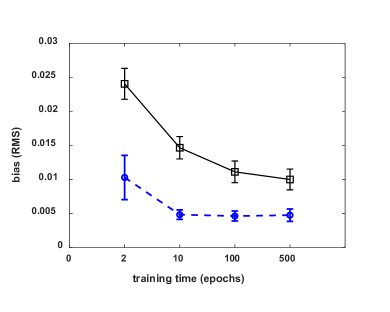
(a) RMS of bias estimate

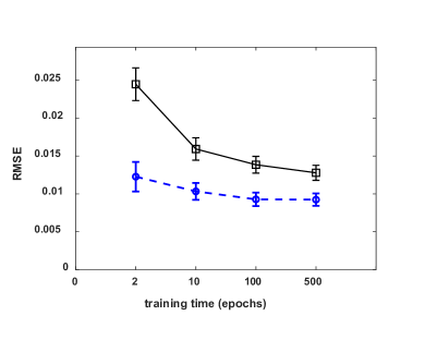
(b) Average RMSE

Figure 1: (a) The root mean square of the estimated bias calculated across different simulation specifications (polynomial factors). Uncorrected is shown with a solid line and black squares, while bias corrected is shown with a dashed line, and blue circles. Error bars are estimated from the different simulation specifications. (b) Similar but instead shows the average root mean squared error (RMSE). The RMSE is calculated for each specification and then averaged across specification.

In order to evaluate algorithm effectiveness, we estimate the algorithm bias for each simulation replication by averaging the difference of the estimated function $\hat{\gamma}(Z)$ with the average of a large set of 1 million independently selected observations, $\gamma_{0}(Z)+\epsilon$, over the 60 samples (with network retraining). The true bias changes for each specification therefore to measure the bias we calculate the root mean square error from zero of the biases across specification. Additionally, we estimate the root mean square error of $\hat{\gamma}(Z)$ and $\gamma_{0}(Z)+\epsilon$.

In figure 1a, we plot the result as a function of training time. We can see right away how the bias correction lowers the expected average bias consistently across the data. The bias correction has the largest effect at lower training times. This can be explained as an increased bias due to increased regularization as the lower training times represent early stopping regularization.

Figure 1a also includes error bars which shows the estimated standard deviation of the root mean square of the bias estimate and the standard deviation of the RMSE. As the two curves in each plot are all over about 3 standard deviations apart, the confidence interval between the bias corrected estimate and the original estimate is generally over $99.5\%$.

Inspecting the plots closely we see that the bias corrected data basically provides the same RMSE at 100 epochs as at 500 epochs, and much more consistency across all of the epochs. This indicates both allowed lowering of required training time and less precision required in determining the best training time.

We also note that the bias correction is shown to provide benefit on average across specifications. For a given specification, the benefit may be negligible or even negative or may be much larger than is shown.

4.4 Discussion

While a variety of possible cross fitting methods can work, the cross-fitting we implemented was done for ease of use in the following manner: The cross-fit data which we will call $v$ is an entirely new sample from the same distribution as $x$. This represents well the case where we have enough data to have both very large training and validation sets.

It also is interesting to note that we observed during our processing that cross-fitting was generally not necessary for this specific problem. Therefore, if we ignore the need for cross-fitting, we can get an alternative description of the debiasing function that applies under the simple assumptions used in the bias correction for this simulation.

Consider that we have a set of functions $b(x)$ where you are finding the weights $\rho$ for each $b(x)$ given a list of residuals. Then given that $\hat{Q}$ in equation 12 is symmetric, the first order conditions to equation 2.1 are a regularized solution of the relationship:

$$\hat{M}=\hat{\rho}\hat{Q}$$

Another solution technique for $\hat{M}=\hat{\rho}\hat{Q}$ would be to solve for $\hat{\rho}$ using a generalized inverse of $\hat{Q}$. We can re-write our variables with matrix notation:

$$\mathbf{B}=[b(X_{1}),...,b(X_{T})]^{\prime}$$ (21)

$$\mathbf{y}=[y(X_{1}),...,y(X_{T})]$$

$$\bm{\hat{\gamma}}=[\hat{\gamma}(X_{1}),...,\hat{\gamma}(X_{T})]$$

Thus we can write this generalized inverse as $\frac{1}{T}\hat{Q}^{+}=[\textbf{B}^{\prime}\textbf{B}]^{+}$. Without cross-fitting, we then can rewrite (7), using $\hat{\alpha}(x)=b(x)^{\prime}\hat{\rho}$, as

$$\frac{1}{N}\sum_{i=1}^{N}\mathbf{\hat{\gamma}}(Z_{i})+[\frac{1}{N}\sum_{i=1}^{N}b(Z_{i})]^{\prime}[\textbf{B}^{\prime}\textbf{B}]^{+}\textbf{B}^{\prime}[\mathbf{y}-\bm{\hat{\gamma}}]$$ (22)

Inspecting this equation, we can set $\hat{\phi}=[\textbf{B}^{\prime}\textbf{B}]^{+}\textbf{B}^{\prime}[\mathbf{y}-\bm{\hat{\gamma}}]$ to be the coefficients of a least squares regression of the residuals on B, with the caveat that $\hat{Q}$ is likely not invertible and thus must be solved using regularization (e.g. a pseudo-inverse on $\hat{Q}$ or Lasso regression on the whole equation). Then the debiased estimator is $\frac{1}{N}\sum_{i=1}^{N}[\mathbf{\hat{\gamma}}(Z_{i})+b(Z_{i})^{\prime}\hat{\phi}]$, where the bias correction is now the coefficients $\hat{\phi}$ on the residuals applied to the test data dictionary $b(Z_{i})$.

The test provided here was evaluated with a few different algorithms and, perhaps surprisingly, we found that with appropriately tuned regularization parameters the debias function worked equally well regardless of the method used.

5 Conclusions

In this paper we have provided debiased machine learning estimators of parameters when there is a covariate shift. We developed a method to debias functionals of trained machine learning algorithms under covariate shift. With cross-fitting the methods were shown to be asymptotically normal as the sample size grows for a variety of regression learners, including neural nets and Lasso. For Lasso regression it was shown that cross-fitting was not needed for these results.

We evaluated the cross-fit method in a relatively simple simulation generated using polynomial coefficients and a neural network with explicit regularization for fitting. The results strongly indicated that the debiased machine learner described here effectively removes the bias.

A significant caveat to consider is that the proposed methodology requires averaging over a reasonable large z sample, and a substantial amount of z data may be required for accurate results. Importantly, without enough averaging, the noise in the bias correction would likely make the results look worse. Because of this, the proposed methodology requires additional computation, which may become significant depending on the dataset sizes.

We believe these results show promise and in future work these methods could be extended to other settings, for example ’counterfactual averages’, or data classification.

References

- [1] Hyojin Bahng, Ali Jahanian, Swami Sankaranarayanan, and Phillip Isola. Exploring visual prompts for adapting large-scale models, 2022.
- [2] Jelena Bradic, Victor Chernozhukov, Whitney K. Newey, and Yinchu Zhu. Minimax semiparametric learning with approximate sparsity, 2022.
- [3] Sara Bühlmann, Peter; Van De Geer. Statistics for High-Dimensional Data. Springer, 2011.
- [4] Victor Chernozhukov, Denis Chetverikov, Mert Demirer, Esther Duflo, Christian Hansen, Whitney Newey, and James Robins. Double/debiased machine learning for treatment and structural parameters. The Econometrics Journal, 21(1):C1–C68, 01 2018.
- [5] Victor Chernozhukov, Whitney K Newey, Victor Quintas-Martinez, and Vasilis Syrgkanis. Automatic debiased machine learning via neural nets for generalized linear regression. arXiv preprint arXiv:2104.14737, 2021.
- [6] Victor Chernozhukov, Whitney K Newey, and Rahul Singh. Automatic debiased machine learning of causal and structural effects. Econometrica, 90(3):967–1027, 2022.
- [7] Marvin Gruber. mproving Efficiency by Shrinkage: The James–Stein and Ridge Regression Estimator. Boca Raton: CRC Pres, 1998.
- [8] T. Hastie, R. Tibshirani, and J.H. Friedman. The Elements of Statistical Learning: Data Mining, Inference, and Prediction. Springer series in statistics. Springer, 2009.
- [9] V Joseph Hotz, Guido W Imbens, and Julie H Mortimer. Predicting the efficacy of future training programs using past experiences at other locations. Journal of Econometrics, 125(1-2):241–270, 2005.
- [10] Peter Kennedy. A Guide to Econometrics (Fifth ed.). Cambridge: The MIT Press., 2003.
- [11] Pang Wei Koh, Shiori Sagawa, Henrik Marklund, Sang Michael Xie, Marvin Zhang, Akshay Balsubramani, Weihua Hu, Michihiro Yasunaga, Richard Lanas Phillips, Irena Gao, Tony Lee, Etienne David, Ian Stavness, Wei Guo, Berton Earnshaw, Imran Haque, Sara M Beery, Jure Leskovec, Anshul Kundaje, Emma Pierson, Sergey Levine, Chelsea Finn, and Percy Liang. Wilds: A benchmark of in-the-wild distribution shifts. In Marina Meila and Tong Zhang, editors, Proceedings of the 38th International Conference on Machine Learning, volume 139 of Proceedings of Machine Learning Research, pages 5637–5664. PMLR, 18–24 Jul 2021.
- [12] Cong Ma, Reese Pathak, and Martin J. Wainwright. Optimally tackling covariate shift in rkhs-based nonparametric regression, 2022.
- [13] Reese Pathak, Cong Ma, and Martin J. Wainwright. A new similarity measure for covariate shift with applications to nonparametric regression, 2022.
- [14] Judea Pearl and Elias Bareinboim. Transportability of causal and statistical relations: A formal approach. In Twenty-fifth AAAI conference on artificial intelligence, 2011.
- [15] Joaquin Quiñonero-Candela, Masashi Sugiyama, Anton Schwaighofer, and Neil D Lawrence. Dataset shift in machine learning| the mit press, 2008.
- [16] Hidetoshi Shimodaira. Improving predictive inference under covariate shift by weighting the log-likelihood function. Journal of Statistical Planning and Inference, 90(2):227–244, 2000.
- [17] Rahul Singh, Liyuan Xu, and Arthur Gretton. Kernel methods for causal functions: Dose, heterogeneous, and incremental response curves. arXiv preprint arXiv:2010.04855, 2020.