1D non-LTE corrections for chemical abundance analyses
of very metal-poor stars

Abstract

Detailed chemical abundances of very metal-poor (VMP, [Fe/H] $<-2$) stars are important for better understanding the First Stars, early star formation and chemical enrichment of galaxies. Big on-going and coming high-resolution spectroscopic surveys provide a wealth of material that needs to be carefully analysed. For VMP stars, their elemental abundances should be derived based on the non-local thermodynamic equilibrium (non-LTE = NLTE) line formation because low metal abundances and low electron number density in the atmosphere produce the physical conditions favorable for the departures from LTE. The galactic archaeology research requires homogeneous determinations of chemical abundances. For this purpose, we present grids of the 1D-NLTE abundance corrections for lines of Na i, Mg i, Ca i, Ca ii, Ti ii, Fe i, Zn i, Zn ii, Sr ii, and Ba ii in the range of atmospheric parameters that represent VMP stars on various evolutionary stages and cover effective temperatures from 4000 to 6500 K, surface gravities from $\rm log~{}g$ = 0.5 to $\rm log~{}g$ = 5.0, and metallicities $-5.0\leq$ [Fe/H] $\leq-2.0$. The data is publicly available, and we provide the tools for interpolating in the grids online.

1 Introduction

Very metal-poor (VMP, [Fe/H] $<-2$) stars are fossils of the early epochs of star formation in their parent galaxy. Their detailed elemental abundances are of extreme importance for understanding the nature of the First Stars, uncovering the initial mass function and the metallicity distribution function of the galaxy, testing the nuclesynthesis theory predictions and the galactic chemical evolution models (Beers & Christlieb, 2005; Frebel & Norris, 2015; Woosley et al., 2019; Kobayashi et al., 2020). Since 1980th, the number of discovered VMP star candidates has grown tremendously thanks to the wide-angle spectroscopic and photometric surveys, such as HK (Beers et al., 1985, 1992), HES (Hamburg/ESO, Christlieb et al., 2002), RAVE (Steinmetz et al., 2006), SMSS (SkyMapper Southern Sky, Keller et al., 2007), SEGUE/SDSS (Yanny et al., 2009), LAMOST (Deng et al., 2012). The survey Pristine has been specially designed for efficient searching VMP stars (Starkenburg et al., 2017). Using the narrow-band photometric filter centered on the Ca ii H & K lines makes possible to successfully predict stellar metallicities (Youakim et al., 2017; Venn et al., 2020).

The number of confirmed VMP stars is substantially lower than the number of candidates because the verification of very low metallicity requires the high-resolution follow-ups. The SAGA (Stellar Abundances for Galactic Archaeology) database (Suda et al., 2008) includes about 1390 Galactic stars with [Fe/H] $\leq-2$, for which their metallicities were derived from the R = $\lambda/\Delta\lambda\geq 20\,000$ spectra. The 470 stars of them have [Fe/H] $\leq-3$, and 28 stars are ultra metal-poor (UMP, [Fe/H] $\leq-4$). A burst in the number of VMP stars with detailed elemental abundances derived is expected with the launch of the WEAVE (WHT Enhanced Area Velocity Explorer) project (see a description in Dalton et al., 2014, science observations start in November of 2022). A vast amount of spectral data will be taken with the coming 4-metre Multi-Object Spectroscopic Telescope (4MOST, de Jong et al., 2019).

Abundance ratios among the elements of different origin, such as Mg and Fe, for stellar samples covering broad metallicity ranges serve as the observational material for the galactic archaeology research. The simplest and widely applied method to derive elemental abundances is based on using one-dimensional (1D) model atmospheres and the assumption of local thermodynamic equilibrium (LTE), see, for example, the abundance results from the high-resolution spectroscopic survey APOGEE (Majewski et al., 2017; Ahumada et al., 2020). In metal-poor atmospheres, in particular, of cool giants, low total gas pressure and low electron number density lead to departures from LTE that grow towards lower metallicity due to decreasing collisional rates and increasing radiative rates as a result of dropping ultra-violet (UV) opacity. The non-local thermodynamic equilibrium (non-LTE = NLTE) line formation calculations show that the NLTE effects for lines of one chemical species and for different chemical species are different in magnitude and sign, depending on the stellar parameters and element abundances. Ignoring the NLTE effects leads to a distorted picture of the galactic abundance trends and thus to wrong conclusions about the galactic chemical evolution.

The NLTE abundance from a given line in a given star can be obtained by adding the theoretical NLTE abundance correction, which corresponds to the star’s atmospheric parameters, to the LTE abundance derived from the observed spectrum: $\log\varepsilon_{\rm NLTE}=\log\varepsilon_{\rm LTE}+\Delta_{\rm NLTE}$. For a number of chemical species, $\Delta_{\rm NLTE}$ can be taken online from the websites

• INSPECT (http://www.inspect-stars.com) for lines of Li i, Na i, Mg i, Ti i, Fe i- ii, and Sr ii,

• NLTE_MPIA (http://nlte.mpia.de/) for lines of O i, Mg i, Si i, Ca i- ii, Ti i- ii, Cr i, Mn i, Fe i- ii, and Co i,

• http://spectrum.inasan.ru/nLTE/ for lines of Ca i, Ti i- ii, and Fe i.

Extensive grids of the NLTE abundance corrections are provided by Korotin et al. (2015, lines of Ba ii), Reggiani et al. (2019, K i), and Lind et al. (2022, Na i, Mg i, Al i). The NLTE abundance corrections for the selected lines of S i and Zn i in the limited set of atmospheric models were computed by Takeda et al. (2005). Merle et al. (2011) report the NLTE to LTE equivalent width ratios for lines of Mg i, Ca i, and Ca ii in the grid of model atmospheres representing cool giants.

Different approach is a determination of the NLTE abundance directly, by using the synthetic spectrum method and the precomputed departure coefficients, b_i = $n_{i}^{\rm NLTE}/n_{i}^{\rm LTE}$, for the chemical species under investigation. Here, $n_{i}^{\rm NLTE}$ and $n_{i}^{\rm LTE}$ are the statistical equilibrium and the Saha-Boltzmann’s number densities, respectively, for the enery level $i$. Amarsi et al. (2020b) provide the grids of b_i for 13 chemical species (neutral H, Li, C, N, O, Na, Mg, Al, Si, K, Ca, Mn; singly ionized Mn, Ba) across a grid of the classical one-dimensional (1D) MARCS model atmospheres (Gustafsson et al., 2008). This approach is based on using the 1D-NLTE spectral synthesis codes, such as SME (Piskunov & Valenti, 2017) synthV_NLTE (Tsymbal et al., 2019), Turbospectrum (Gerber et al., 2023).

An approach based on three-dimensional (3D) model atmospheres combined with the NLTE line formation is extremely time consuming and, to now, was applied to a few chemical species in the Sun (Steffen et al., 2015; Lind et al., 2017; Amarsi & Asplund, 2017; Amarsi et al., 2018, 2019, 2020a; Gallagher et al., 2020) and the benchmark VMP stars (Amarsi et al., 2016b; Nordlander et al., 2017; Bergemann et al., 2019). Grids of the 3D-NLTE abundance corrections were computed for lines of O i (Amarsi et al., 2016a) and Fe i- ii (Amarsi et al., 2022) using the STAGGER grid of model atmospheres for a limited range of effective temperatures ($T_{\rm eff}$ = 5000-6500 K), surface gravities ($\rm log~{}g$ = 3.0-4.5), and metallicities ([Fe/H] = 0 to $-3$). For the Li i lines, grids of the 3D-NLTE abundance corrections were computed by Mott et al. (2020) and Wang et al. (2021) with the CO⁵BOLD and STAGGER model atmospheres, respectively.

The 3D-NLTE calculations are available for a small number of the chemical elements observed in VMP stars, and they cover only in part the range of relevant atmospheric parameters. Furthermore, as shown by Amarsi et al. (2022) for Fe i, the abundance differences between 3D-NLTE and 1D-NLTE are generally less severe compared with the differences between 3D-NLTE and 1D-LTE and reach 0.2 dex, at maximum (see Figs. 5-7 in their paper). Therefore, calculations of the 1D-NLTE abundance corrections for extended linelists across the stellar parameter range which represents the VMP stars make sense, and they are useful for the galactic archaeology research. Availability and comparison of $\Delta_{\rm NLTE}$ from different independent studies increase a credit of confidence in the spectroscopic NLTE analyses.

This paper presents the 1D-NLTE abundance corrections for lines of 10 chemical species in the grid of MARCS model atmospheres with $T_{\rm eff}$ = 4000-6500 K, $\rm log~{}g$ = 0.5-5.0, and $-5\leq$ [Fe/H] $\leq-2$. We provide the tools for calculating online the NLTE abundance correction(s) for given line(s) and given atmospheric parameters by interpolating in the precomputed grids.

Potential users may take the following advantages of our data compared with the grids of the 1D-NLTE abundance corrections available in the literature.

• Only this study provides extended grids of the NLTE abundance corrections for lines of Zn ii and Ba ii.

• For Ca i and Ca ii, the NLTE calculations were performed with advanced treatment of the Ca i + H i and Ca ii + H i collisions, following Belyaev et al. (2017) and Belyaev et al. (2019), respectively.

• For Zn i and Sr ii, our results are based on advanced treatment of collisions with H i, following Sitnova et al. (2022, Zn i) and Yakovleva et al. (2022, Sr ii). Our grids cover the broader range of $T_{\rm eff}$, $\rm log~{}g$, and [Fe/H] compared to that for Zn i in Takeda et al. (2005) and for Sr ii in the INSPECT database.

• For Ca i–Ca ii, Fe i–Fe ii, and Na i, the developed 1D-NLTE methods have been verified with spectroscopic analyses of VMP stars and have been shown to yield reliable results.

The paper is organised as follows. Section 2 describes our NLTE methods and their verification with observations of VMP stars. New grids of the NLTE abundance corrections are presented in Sect. 3. In Sect. 4, we compare our calculations with those from other studies. Our recommendations and final remarks are given in Sect. 5.

2 NLTE methods and their verification

The present investigation is based on the NLTE methods developed and tested in our earlier studies. Details of the adopted atomic data and the NLTE line formation for Na i, Mg i, Ca i- ii, Ti i-Ti ii, Fe i- ii, Zn i- ii, Sr ii, and Ba ii can be found in the papers cited in Table 1. It is important to note that collisions with hydrogen atoms were treated with the data based on quantum-mechanical calculations. The exceptions are Ti ii and Fe i- ii, for which we adopted the Drawinian rates (Drawin, 1969; Steenbock & Holweger, 1984) scaled by an empirically estimated factor of $S_{\rm H}$ = 1 (Sitnova et al., 2016) and $S_{\rm H}$ = 0.5 (Sitnova et al., 2015; Mashonkina et al., 2017a), respectively.

Table 1: Atomic models used in this study.

Species	Reference	H i collisions
Na i	Alexeeva et al. (2014)	BBD10
Mg i	Mashonkina (2013)	BBS12
Ca i- ii	Mashonkina et al. (2017b),	BVY17
	Neretina et al. (2020)	BVY19
Ti ii	Sitnova et al. (2016)	$S_{\rm H}$ = 1
Fe i- ii	Mashonkina et al. (2011)	$S_{\rm H}$ = 0.5
Zn i- ii	Sitnova et al. (2022)	YB22
Sr ii	Mashonkina et al. (2022)	YBM22
Ba ii	Mashonkina & Belyaev (2019)	BY18

Notes. Collisions with H i are treated following to BBD10 = Barklem et al. (2010), BBS12 = Barklem et al. (2012), BVY17 = Belyaev et al. (2017, Ca i), BVY19 = Belyaev et al. (2019, Ca ii), BY18 = Belyaev & Yakovleva (2018), YB22 = Yakovleva S. A. and Belyaev A. K., as presented in Sitnova et al. (2022), YBM22 = Yakovleva et al. (2022), and Steenbock & Holweger (1984), with using the scaling factor $S_{\rm H}$.

The code detail (Giddings, 1981; Butler, 1984) with the revised opacity package (see the description in Mashonkina et al., 2011) was used to solve the coupled radiative transfer and statistical equilibrium (SE) equations. The obtained LTE and NLTE level populations were then implemented in the code linec (Sakhibullin, 1983) that, for each given spectral line, computes the NLTE curve of growth and finds the shift in the NLTE abundance, which is required to reproduce the LTE equivalent width. Such an abundance shift is referred to as the NLTE abundance correction, $\Delta_{\rm NLTE}=\log\varepsilon_{\rm NLTE}-\log\varepsilon_{\rm LTE}$.

All the calculations were performed using the classical LTE model atmospheres with the standard chemical composition (Gustafsson et al., 2008), as provided by the MARCS website.

Below we provide evidence for a correct treatment of the NLTE line formation for Fe i-Fe ii, Ca i-Ca ii, and Na i in the atmospheres of VMP stars.

Table 2: Distance-based and spectroscopic surface gravities for the Galactic stellar samples from Sitnova et al. (2015) and Mashonkina et al. (2017a).

Star	Gaia eDR3		$T_{\rm eff}$	$\rm log~{}g$	[Fe/H]
	d(pc)	$\rm log~{}g_{\rm d}$	(K)	(Sp)
1	2	3	4	5	6
HD 2796	631.3 (9.3)	1.79 (0.03)	4880	1.55	–2.32
HD 4306	480.6 (7.7)	2.26 (0.03)	4960	2.18	–2.74
HD 8724	425.8 (4.6)	1.77 (0.03)	4560	1.29	–1.76
HD 19373	10.57 (0.02)	4.18 (0.02)	6045	4.24	0.10
HD 22484	13.91 (0.03)	4.03 (0.02)	6000	4.07	0.01
HD 22879	26.07 (0.02)	4.23 (0.02)	5800	4.29	–0.84
HD 24289	211.9 (1.9)	3.79 (0.03)	5980	3.71	–1.94
HD 30562	26.12 (0.03)	4.09 (0.02)	5900	4.08	0.17
HD 30743	36.22 (0.03)	4.13 (0.02)	6450	4.20	–0.44
HD 34411	12.55 (0.02)	4.23 (0.02)	5850	4.23	0.01
HD 43318	36.30 (0.09)	3.90 (0.02)	6250	3.92	–0.19
HD 45067	32.85 (0.05)	3.96 (0.02)	5960	3.94	–0.16
HD 45205	75.59 (0.12)	3.85 (0.02)	5790	4.08	–0.87
HD 49933	29.79 (0.04)	4.17 (0.02)	6600	4.15	–0.47
HD 52711	18.93 (0.02)	4.32 (0.02)	5900	4.33	–0.21
HD 58855	20.38 (0.06)	4.28 (0.02)	6410	4.32	–0.29
HD 59374	57.86 (0.06)	4.29 (0.02)	5850	4.38	–0.88
HD 59984	28.64 (0.03)	3.96 (0.02)	5930	4.02	–0.69
HD 62301	34.07 (0.03)	4.09 (0.02)	5840	4.09	–0.70
HD 64090	27.32 (0.02)	4.60 (0.03)	5400	4.70	–1.73
HD 69897	18.21 (0.03)	4.24 (0.02)	6240	4.24	–0.25
HD 74000	109.8 (0.2)	4.27 (0.02)	6225	4.13	–1.97
HD 76932	21.41 (0.02)	4.09 (0.02)	5870	4.10	–0.98
HD 82943	27.66 (0.02)	4.37 (0.02)	5970	4.37	0.19
HD 84937	73.87 (0.24)	4.15 (0.02)	6350	4.09	–2.16
HD 89744	38.50 (0.06)	3.98 (0.02)	6280	3.97	0.13
HD 90839	12.94 (0.01)	4.33 (0.02)	6195	4.38	–0.18
HD 92855	36.63 (0.03)	4.40 (0.02)	6020	4.36	–0.12
HD 94028	49.39 (0.06)	4.33 (0.02)	5970	4.33	–1.47
HD 99984	51.50 (0.10)	3.72 (0.02)	6190	3.72	–0.38
HD 100563	26.86 (0.04)	4.25 (0.02)	6460	4.32	0.06
HD 102870	11.00 (0.02)	4.06 (0.02)	6170	4.14	0.11
HD 103095	9.17 (0.00)	4.66 (0.03)	5130	4.66	–1.26
HD 105755	83.31 (0.10)	4.05 (0.02)	5800	4.05	–0.73
HD 106516	22.32 (0.40)	4.38 (0.03)	6300	4.44	–0.73
HD 108177	105.9 (0.2)	4.25 (0.02)	6100	4.22	–1.67
HD 108317	192.7 (1.1)	2.81 (0.03)	5270	2.96	–2.18
HD 110897	17.55 (0.01)	4.36 (0.02)	5920	4.41	–0.57
HD 114710	9.19 (0.01)	4.45 (0.02)	6090	4.47	0.06
HD 115617	8.53 (0.01)	4.35 (0.03)	5490	4.40	–0.10
HD 122563	318.6 (3.4)	1.32 (0.03)	4600	1.32	–2.63
HD 128279	130.4 (0.5)	3.01 (0.03)	5200	3.00	–2.19
HD 134088	39.23 (0.04)	4.36 (0.02)	5730	4.46	–0.80
HD 134169	53.88 (0.39)	4.09 (0.02)	5890	4.02	–0.78
HD 138776	76.11 (0.15)	4.17 (0.03)	5650	4.30	0.24
HD 140283	61.32 (0.10)	3.73 (0.02)	5780	3.70	–2.46
HD 142091	29.96 (0.07)	3.10 (0.03)	4810	3.12	–0.07
HD 142373	15.89 (0.02)	3.90 (0.02)	5830	3.96	–0.54
HD 218857	346.2 (2.3)	2.57 (0.03)	5060	2.53	–1.92
HE0011-0035	7080 (1308)	2.32 (0.16)	4950	2.00	–3.04
HE0039-4154	7032 (720)	1.80 (0.09)	4780	1.60	–3.26
HE0048-0611	6434 (1253)	2.69 (0.17)	5180	2.70	–2.69
HE0122-1616	5582 (1103)	2.94 (0.17)	5200	2.65	–2.85
HE0332-1007	12774 (2892)	1.47 (0.20)	4750	1.50	–2.89
HE0445-2339	6673 (624)	2.03 (0.09)	5165	2.20	–2.76
HE1356-0622	7770 (1507)	1.88 (0.17)	4945	2.00	–3.45

Notes. The errors of the Gaia eDR3 distances and $\rm log~{}g_{\rm d}$ are indicated in parentheses.

Table 3: continued

– Distance-based and spectroscopic surface gravities for the Galactic stellar samples from Sitnova et al. (2015) and Mashonkina et al. (2017a). Star Gaia eDR3 $T_{\rm eff}$ $\rm log~{}g$, [Fe/H] d(pc) $\rm log~{}g_{\rm d}$ (K) Sp 1 2 3 4 5 6 HE1357-0123 14890 (4225) 1.30 (0.25) 4600 1.20 –3.92 HE1416-1032 8244 (1635) 2.15 (0.17) 5000 2.00 –3.23 HE2244-2116 7703 (2213) 2.67 (0.25) 5230 2.80 –2.40 HE2249-1704 10602 (2771) 1.86 (0.23) 4590 1.20 –2.94 HE2252-4225 9265 (2354) 1.93 (0.22) 4750 1.55 –2.76 HE2327-5642 4711 (308) 2.25 (0.06) 5050 2.20 –2.92 BD+07^∘4841 156.0 (0.4) 4.30 (0.02) 6130 4.15 –1.46 BD+09^∘0352 158.1 (0.5) 4.16 (0.02) 6150 4.25 –2.09 BD+24^∘1676 250.2 (1.1) 4.08 (0.02) 6210 3.90 –2.44 BD+29^∘2091 87.69 (0.15) 4.59 (0.02) 5860 4.67 –1.91 BD+37^∘1458 143.9 (0.3) 3.56 (0.03) 5500 3.70 –1.95 BD+66^∘0268 49.55 (0.04) 4.66 (0.03) 5300 4.72 –2.06 BD$-04^{\circ}$3208 174.1 (0.6) 4.12 (0.02) 6390 4.08 –2.20 BD$-11^{\circ}$0145 2055 ( 80) 1.66 (0.04) 4900 1.73 –2.18 BD$-13^{\circ}$3442 210.6 (1.4) 4.12 (0.02) 6400 3.95 –2.62 CD$-24^{\circ}$1782 469.0 (3.7) 2.76 (0.03) 5140 2.62 –2.72 BS16550-0087 8253 (1052) 1.58 (0.11) 4750 1.50 –3.33 G090-003 250.8 (1.1) 3.89 (0.02) 6007 3.90 –2.04

Notes. The errors of the Gaia eDR3 distances and $\rm log~{}g_{\rm d}$ are indicated in parentheses.

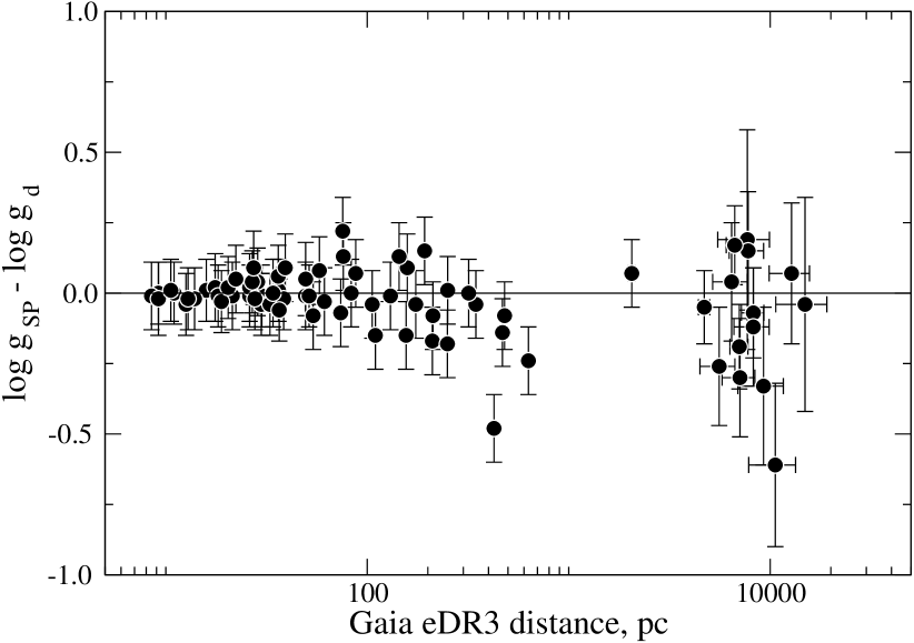
Figure 1: The differences between spectroscopic and distance-based surface gravities depending on the Gaia eDR3 distance for the Galactic stellar samples from Sitnova et al. (2015) and Mashonkina et al. (2017a).

2.1 Spectroscopic versus Gaia eDR3 distances

Iron is represented in the VMP stars by the two ionization stages, which are used in many studies to determine spectroscopic surface gravities ($g_{\rm Sp}$) from the requirement that abundances from lines of Fe i and Fe ii in a given star must be equal. The surface gravity can also be derived from distance; this is the distance-based surface gravity, $g_{\rm d}$. If $g_{\rm Sp}$ based on the NLTE calculations and $g_{\rm d}$ are obtained to be consistent within the error bars, this means that the calculations for Fe i-Fe ii are correct.

Sitnova et al. (2015) and Mashonkina et al. (2017a) derived the surface gravities for the two Galactic stellar samples using photometric effective temperatures and the NLTE analysis of the Fe i and Fe ii lines. Using the Gaia eDR3 parallaxes corrected according to Lindegren et al. (2021), we calculated distances from the maximum of the distance probability distribution function, as recommended by Bailer-Jones (2015), and then $\rm log~{}g_{\rm d}$ from the relation

$$\mathrm{log}\,g_{\rm d}=-10.607+\mathrm{log}\,M+4\,\mathrm{log}\,T_{\rm eff}-$$

$$0.4\,[4.74-(V+BC+5-5\,\mathrm{log\,d}-A_{V})]$$

Here, $M$ is a star’s mass, $A_{V}$ is an interstellar extintion in the V-band, $BC$ is a bolometric correction which was calculated by interpolation in the grid of Bessell et al. (1998). The atmospheric parameters and $A_{V}$ were taken from Sitnova et al. (2015) and Mashonkina et al. (2017a). Stellar masses and $V$ magnitudes for the Sitnova et al. (2015) sample are listed in their Table 5 and 2, respectively. For the stellar sample of Mashonkina et al. (2017a), the $V$ magnitudes are listed in their Table 5. For each VMP giant, we adopt $M=0.8M_{\odot}$.

Statistical error of the distance-based surface gravity was computed as the quadratic sum of errors of the star’s distance, effective temperature, mass, visual magnitude, and $BC$. We assumed the stellar mass error as $\sigma_{M}=0.1M_{\odot}$ and took the effective temperature errors, $\sigma_{T}$, from Sitnova et al. (2015) and Mashonkina et al. (2017a). The total error is dominated by $\sigma_{M}$ for the nearby stars and by the distance error, $\sigma_{\rm d}$, for the distant objects.

Table 2 lists the obtained Gaia eDR3 distances and $\rm log~{}g_{\rm d}$ values, as well as the spectroscopic surface gravities from Sitnova et al. (2015) and Mashonkina et al. (2017a). The differences log $g_{\rm Sp}$ – $\rm log~{}g_{\rm d}$ are shown in Fig. 1. The majority of our stars lie within 631 pc from the Sun, and their spectroscopic surface gravities are found to be consistent within the error bars with the distance-based ones. A clear outlier is HD 8724, with log $g_{\rm Sp}$ – $\rm log~{}g_{\rm d}=-0.48$. We note that the discrepancy between log $g_{\rm Sp}$ and $\rm log~{}g_{\rm d}$ has reduced compared to $-0.76$ dex obtained for HD 8724 by Mashonkina et al. (2017a) using the Gaia DR1 parallax (Gaia Collaboration et al., 2016). However, it is still greater than the error of spectroscopic surface gravity, $\sigma_{\log g{\rm(sp)}}$ = 0.24 dex. Formal calculation of $\sigma_{\log g{\rm(d)}}$ leads to 0.07 dex (Table 2), however, astrometric_excess_noise_sig = 6.005 and astrometric_chi2_al = 419.84 indicated by Lindegren et al. (2021) for HD 8724 suggest an unreliable solution for the Gaia eDR3 parallax.

For 15 distant stars, with d $>$ 2 kpc, the errors of $\rm log~{}g_{\rm d}$ grow. Nevertheless, the spectroscopic surface gravities are consistent, on average, with the distance-based ones.

Thus, our NLTE method for Fe i/Fe ii is reliable and can be used for determinations of surface gravities, in particular, for distant stars with large distance errors.

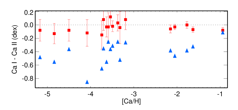
Figure 2: NLTE (red squares) and LTE (blue triangles) differences between the Ca i- and Ca ii-based abundances for the stellar samples from Mashonkina et al. (2017b) and Sitnova et al. (2019).

2.2 Ca i versus Ca ii

A firm argument for a correct treatment of the NLTE line formation for Ca i-Ca ii can be obtained from a comparison of the NLTE abundances from lines of the two ionization stages. Mashonkina et al. (2017b) report the LTE and NLTE abundances from lines of Ca i and Ca ii 8498 Å for five reference stars with well-determined atmospheric parameters in the $-2.7<$ [Fe/H] $<-1.3$ metallicity range and find fairly consistent NLTE abundances, while the LTE abundance difference between Ca i and Ca ii 8498 Å grows in absolute value towards lower metallicity and reaches $-0.45$ dex for [Fe/H] = $-2.62$, see their Fig. 6.

Sitnova et al. (2019) studied the UMP stars and improved their atmospheric parameters using an extensive method based on the colour-$T_{\rm eff}$ calibrations, NLTE fits of the Balmer line wings, and Gaia DR2 trigonometric parallaxes. For each star, the derived effective temperature and surface gravity were checked by inspecting the Ca i/Ca ii NLTE ionization equilibrium and by comparing the star’s position in the $\rm log~{}g-T_{\rm eff}$ plane with the theoretical isochrones of 12 and 13 Gyr.

The abundance differences between the two ionization stages from the NLTE and LTE calculations of Mashonkina et al. (2017b) and Sitnova et al. (2019) are displayed in Fig. 2. Nowhere, the NLTE abundance difference Ca i – Ca ii exceeds 0.15 dex, while the LTE abundances from lines of Ca ii are systematically lower compared with that from Ca i, by up to 0.85 dex. Thus, the NLTE results obtained using our NLTE method for Ca i- ii (Mashonkina et al., 2017b) can be trusted.

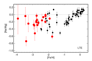
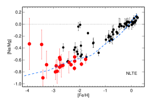
Figure 3: [Na/Mg] LTE (left panel) and NLTE (right panel) abundance ratios for the dwarf stellar sample from Zhao et al. (2016, small black circles) and the giant sample from Mashonkina et al. (2017c, large red circles). The NLTE abundance ratios are well reproduced by the chemical evolution model of Kobayashi et al. (2020, dashed curve).

2.3 Na i resonance lines in VMP stars

Figure 3 displays the [Na/Mg] abundance ratios in the wide range of metallicities from the LTE and NLTE calculations of Zhao et al. (2016) and Mashonkina et al. (2017c). For [Fe/H] $>-1$, both LTE and NLTE data form a well-defined upward trend, with a small star-to-star scatter for the stars of close metallicity. The situation is very different in LTE and NLTE for [Fe/H] $<-1$. In LTE, the [Na/Mg] ratios reveal a big scatter, which is substantially reduced in the NLTE calculations. An explanation lies mostly with the NLTE effects for lines of Na i. For Mg, the differences between the NLTE and LTE abundances do not exceed 0.1 dex.

For [Fe/H] $>-1$, the Na abundances were derived by Zhao et al. (2016) from the Na i 5682, 5688, 6154, 6160 5895 Å subordinate lines, which are slightly affected by NLTE, with negative $\Delta_{\rm NLTE}$ of $\precsim$0.1 dex, in absolute value. In the lower metallicity stars, sodium is observed in the Na i 5889, 5895 Å resonance lines only. They are subject to strong NLTE effects, with $\Delta_{\rm NLTE}$ depending on the atmospheric parameters and the Na abundance itself. For different stars, $\Delta_{\rm NLTE}$ varies between $-0.1$ and $-0.6$ dex (Mashonkina et al., 2017c). Removing the star-to-star scatter of the [Na/Mg] NLTE abundance ratios for [Fe/H] $<-1$ can serve as a circumstantial evidence for the line formation to be treated correctly.

Taking advantage of the obtained Galactic NLTE [Na/Mg] trend, we found that the modern nuclesynthesis and Galactic chemical evolution (GCE) calculations, which are represented in Fig. 3 (right panel) by the GCE model of Kobayashi et al. (2020), predict correctly contributions from the core-collapse supernovae (SNeII) and the asymptotic giant branch (AGB) stars to production of Mg and Na during the Galaxy history.

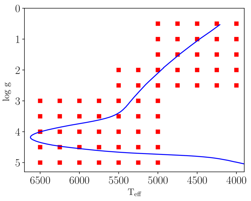
Figure 4: Stellar parameter range covered by our tables of the NLTE abundance corrections is shown by squares. The solid curve is the isochrone of 12 Gyr, [Fe/H] = $-2$, and [$\alpha$/Fe] = 0.4 from Dotter et al. (2008).

3 Grids of the NLTE abundance corrections

By request of the Pristine collaboration (Starkenburg et al., 2017), the NLTE abundance corrections were computed for the lines which can be detected in spectra of VMP stars, that is, for the [Fe/H] $\leq-2$ range. We focused, in particular, on the spectral ranges observed by WEAVE, that is 4040-4650 Å, 4750-5450 Å, and 5950-6850 Å for the high-resolution ($R=\lambda/\Delta\lambda$ = 20 000) observations and 3660-9590 Å for the $R$ = 5000 observations, and 4MOST , that is 3926-4350 Å, 5160-5730 Å, and 6100-6790 Å for the high-resolution spectrograph (HRS, $R\simeq$ 20 000) and 3700-9500 Å for the low-resolution spectrograph (LRS, $R\simeq$ 4000-7500). We selected 4 / 15 / 28 / 4 / 54 / 262 / 7 / 2 / 2 / 5 lines of Na i / Mg i / Ca i / Ca ii / Ti ii / Fe i / Zn i / Zn ii / Sr ii / Ba ii.

The range of atmospheric parameters was selected to represent metal-poor stars on various evolutionary stages, from the main sequence to the red giant branch (RGB); see the isochrone of 12 Gyr, [Fe/H] = $-2$, and [$\alpha$/Fe] = 0.4 from Dotter et al. (2008) in Fig. 4. The NLTE calculations were performed in the following ranges of effective temperature and surface gravity:

$T_{\rm eff}$ = 4000 to 4750 K for $\rm log~{}g$ = 0.5 to 2.5;

$T_{\rm eff}$ = 5000 K for $\rm log~{}g$ = 0.5 to 5.0;

$T_{\rm eff}$ = 5250 to 5500 K for $\rm log~{}g$ = 2.0 to 5.0;

$T_{\rm eff}$ = 5750 to 6500 K for $\rm log~{}g$ = 3.0 to 5.0.

Metallicity range is $-5.0\leq$ [Fe/H] $\leq-2.0$.

The nodes of the NLTE abundance correction grids correspond to the nodes of the MARCS model grid. Therefore, $T_{\rm eff}$ varies with a step of 250 K, $\rm log~{}g$ with a step of 0.5, and [Fe/H] with a step of 0.5. The MARCS website does not provide models with [Fe/H] = $-3.5$ and $-4.5$. The missing models were calculated by interpolating between the [Fe/H] = $-3$ and $-4$ and between the [Fe/H] = $-4$ and $-5$ models. We applied the FORTRAN-based interpolation routine written by Thomas Masseron and available on the MARCS website.

For Fe i- ii and Zn i- ii, the SE calculations were performed with [Element/Fe] = 0.0; for Mg i and Ti ii with [Element/Fe] = 0.4 and 0.3, respectively.

For Na i, Ca i, Ca ii, Sr ii, and Ba ii, the NLTE effects are sensitive to not only $T_{\rm eff}$/$\rm log~{}g$/[Fe/H], but also the element abundance used in the SE calculations. Therefore, the grids of the NLTE corrections are 4-dimensional where [Element/Fe] takes the following numbers:

[Na/Fe] = $-0.6$, $-0.3$, 0.0, 0.3, 0.6;

[Ca/Fe] = 0.0 and 0.4;

[Sr/Fe] = $-1.0$, $-0.5$, 0.0, 0.5, 1.0 for the dwarf model atmospheres,

[Sr/Fe] = $-1.5$, $-1.0$, $-0.5$, 0.0, 0.5 for the giant model atmospheres;

[Ba/Fe] = $-1.0$, $-0.5$, 0.0, 0.5 for the dwarf model atmospheres,

[Ba/Fe] = $-1.5$, $-1.0$, $-0.5$, 0.0, 0.5 for the giant model atmospheres.

The website INASAN_NLTE provides the tools for calculating online the NLTE abundance correction(s) for given spectral line(s) and atmospheric parameters $T_{\rm eff}$, $\rm log~{}g$, [Fe/H], [Element/Fe] by an interpolation in the NLTE correction grids.

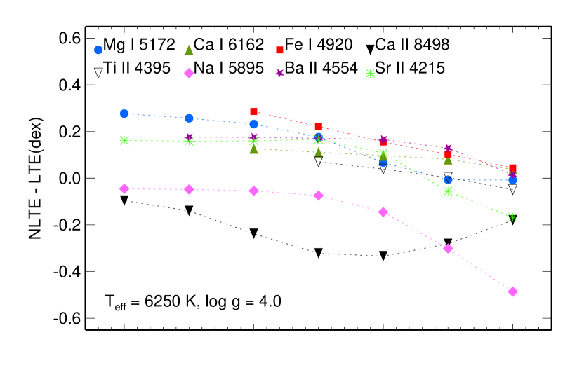
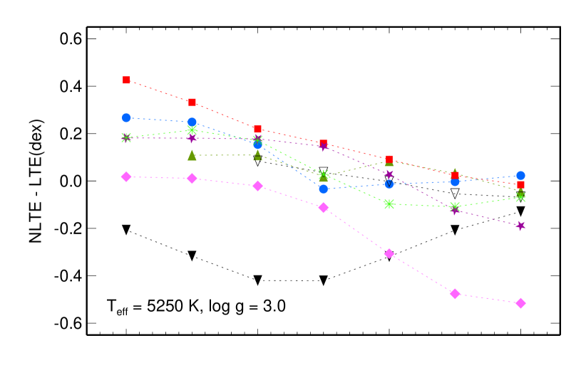
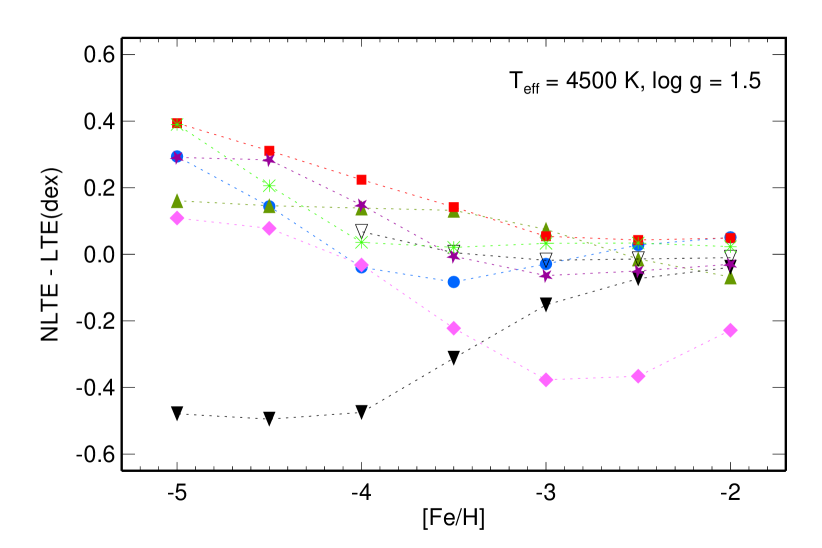
Figure 5: NLTE abundance corrections for lines of Na i (rhombi), Mg i (circles), Ca i (triangles), Ca ii (filled inverted triangles), Ti ii (open inverted triangles), Fe i (squares), Sr ii (asterisks), and Ba ii (five-pointed star) as a function of metallicity in the models with $T_{\rm eff}$/$\rm log~{}g$ = 6250/4.0 (top panel), 5250/3.0 (middle panel), and 4500/1.5 (bottom panel). Everywhere in the NLTE calculations, [Element/Fe] = 0 was adopted.

3.1 NLTE corrections depending on atmospheric parameters

Figure 5 displays the NLTE abundance corrections predicted for representative lines of different chemical species in VMP stars on different evolutionary stages, namely, the turn-off (TO, $T_{\rm eff}$/$\rm log~{}g$ = 6250/4.0), the bottom red giant branch (bRGB, 5250/3.0), and the RGB (4500/1.5). For each line, $\Delta_{\rm NLTE}$ depends on $T_{\rm eff}$, $\rm log~{}g$ and [Fe/H]. Therefore, neglecting the NLTE effects distorts the galactic abundance trends. In the same atmosphere, different lines have the NLTE corrections of different magnitude and sign. Therefore, the star’s element abundance pattern derived under the LTE assumption does not reflect correctly relative contributions of different nuclesynthesis sources.

The sign of $\Delta_{\rm NLTE}$ is determined by the mechanisms that produce the departures from LTE for lines of a given species in given physical conditions.

In the stellar parameter range with which we concern, Mg i, Ca i, and Fe i are the minority species in the line formation layers, and they are subject to the ultra-violet (UV) overionization, resulting in depleted atomic level populations, weakened lines, and positive NLTE abundance corrections (see Mashonkina et al., 1996, 2007, 2011, for detailed analyses). The intensity of the ionizing UV radiation increases with decreasing metallicity, resulting in growing departures from LTE.

Na i is also the minority species, however, due to low photoionization cross-sections of its ground state, the main NLTE mechanism is a "photon suction" process (Bruls et al., 1992) which produces overpopulation of the neutral stage, resulting in strengthened Na i lines and negative NLTE abundance corrections. Photon suction is connected with collisional processes that couple the high-excitation levels of Na i with the singly ionized stage. In contrast to the radiative processes, an influence of collisional processes on the statistical equilibrium of Na i is weakened with decreasing metallicity, and $\Delta_{\rm NLTE}$ for Na i 5895 Å decreases in absolute value and becomes even slightly positive for [Fe/H] $\leq-4.5$ in the 4500/1.5 models.

The NLTE effects for the majority species Ca ii, Ti ii, Sr ii, and Ba ii are driven by the bound-bound (b-b) transitions. For an individual line, the sign and magnitude of $\Delta_{\rm NLTE}$ depend on the physical conditions and the transition where the line arises. Ca ii 8498 Å arises in the transition $3d\,^{2}{\rm D}_{\rm 3/2}$ – $4p\,^{2}{\rm P}^{\circ}_{\rm 3/2}$. The upper level is depopulated in the atmospheric layers where the core of Ca ii 8498 Å forms via photon loss in the wings of the Ca ii 3933, 3968 Å resonance lines and the 8498, 8542, 8668 Å infra-red (IR) triplet lines. The Ca ii 8498 Å line core is strengthened because the line source function drops below the Planck function, resulting in negative $\Delta_{\rm NLTE}$ (Mashonkina et al., 2007). In the [Fe/H] = $-2$ models, Ca ii 8498 Å is very strong with a total absorption dominated by the line wings that form in deep atmospheric layers where the NLTE effects are small. With decreasing [Fe/H] (and Ca abundance, too) the line wings are weakened, and $\Delta_{\rm NLTE}$ grows in absolute value. In the 6250/4.0 and 5250/3.0 models, $\Delta_{\rm NLTE}$ decreases in absolute value for [Fe/H] $\leq-3.5$ because of shifting the formation depths for Ca ii 8498 Å in deep atmospheric layers.

Owing to a complex atomic term structure, the levels of Ti ii are tightly coupled to each other and to the ground state via radiative and collisional processes, and the NLTE corrections for the Ti ii lines are slightly positive in the stellar parameter range with which we concern (Sitnova et al., 2016): $\Delta_{\rm NLTE}\precsim$ 0.1 dex for Ti ii 4395 Å.

Mashonkina & Gehren (2001) and Mashonkina et al. (1999) predicted theoretically that NLTE may either strengthen or weaken the lines of Sr ii and Ba ii, depending on the stellar parameters and elemental abundance. For example, in the 6250/4.0 models, $\Delta_{\rm NLTE}$ is positive for Ba ii 4554 Å over full range of [Fe/H] = $-2$ down to $-4.5$, while, for Sr ii 4215 Å, $\Delta_{\rm NLTE}$ is negative when [Fe/H] $\geq-2.5$ and positive for the more metal-deficient atmospheres. In the RGB atmospheres, both Sr ii 4215 Å and Ba ii 4554 Å are very strong until metallicity decreases to [Fe/H] = $-3.5$, and the NLTE corrections are small. For the lower metallicity, $\Delta_{\rm NLTE}$ is positive for both lines and grows with decreasing [Fe/H].

For lines of Zn i, the NLTE abundance corrections depending on atmospheric parameters are discussed by Sitnova et al. (2022).

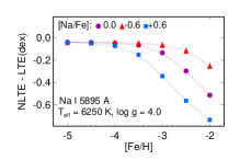
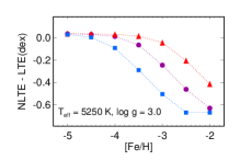
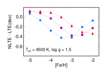
Figure 6: NLTE abundance corrections for Na i 5895 Å depending on the element abundance in the models representing atmospheres of the TO, bRGB, and RGB stars. The circles, triangles, and squares correspond to [Na/Fe] = 0.0, $-0.6$, and +0.6, respectively.

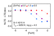
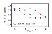
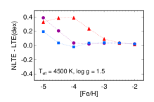
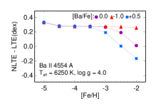
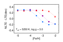
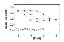
Figure 7: The same as in Fig. 6 for Sr ii 4215 Å (top row) and Ba ii 4554 Å (bottom row). The circles, triangles, and squares correspond to [Element/Fe] = 0.0, $-1.0$, and +0.5, respectively.

3.2 NLTE corrections depending on elemental abundances

The stars of close metallicity in the [Fe/H] $<-2$ range reveal a substantial scatter of the Na, Sr, and Ba abundances (see, for example Cohen et al., 2013). Exactly for Na i, Sr ii, and Ba ii the NLTE effects depend strongly on not only atmospheric parameters, but also the element abundance. Therefore in order to interpret correctly the chemical evolution of Na, Sr, and Ba, abundance analyses of VMP samples should be based on the NLTE abundances.

Figure 6 shows that, for the TO and bRGB stars, the LTE analysis overestimates the Na abundances, by the quantity which is greater for the Na-enhanced than for Na-poor star. The difference in $\Delta_{\rm NLTE}$ exceeds 0.4 dex for [Fe/H] = $-2.5$ and reduces towards the lower [Fe/H]. The same is true for the RGB stars with [Fe/H] $\leq-3.5$, but the situation is more complicated for the higher metallicities. For [Fe/H] $>-3$, the Na i 5895 Å line is very strong in the Na-enhanced cool atmospheres, and the total line absorption is dominated by the line wings that form in deep atmospheric layers affected only weakly by NLTE. Accounting for the NLTE effects for the Na i lines reduces substantially the abundance discrepancies found for stellar samples in LTE, as well illustrated by Fig. 3.

Using the same atmospheric parameters, LTE may either overestimate, or underestimate abundances of Sr and Ba depending on the elemental abundances, as shown in Fig. 7. For [Fe/H] $<-2$, the NLTE abundance corrections for Sr ii 4215 Å and Ba ii 4554 Å are positive in the Sr- and Ba-poor atmospheres, while they can be negative for the Sr- and Ba-enhanced atmospheres. Accounting for the NLTE effects can reduce the abundance discrepancies found for stellar samples in LTE, by more than 0.4 dex for Sr in the TO [Fe/H] = $-2.5$ stars and for Ba in the bRGB [Fe/H] = $-2.5$ stars.

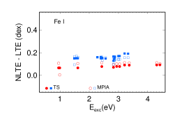
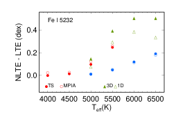
Figure 8: NLTE abundance corrections for lines of Fe i from our calculations (this study = TS, filled circles and squares), the NLTE_MPIA database (open circles and squares), and Amarsi et al. (2022, triangles). Left panel: lines of various $E_{\rm exc}$ in the model atmospheres 6350/4.09/$-2.18$ (circles) and 4630/1.28/$-2.99$ (squares). Right panel: Fe i 5232 Å in the model atmospheres with [Fe/H] = $-3$ for $\rm log~{}g$ = 2.5 (red symbols) and 4.0 (blue and green symbols). The filled and open triangles corresponds to the 3D NLTE and 1D NLTE calculations, respectively.

3.3 NLTE corrections for different type model atmospheres

The model atmospheres computed with different codes produce, as a rule, very similar atmospheric structures and spectral energy distributions for common atmospheric parameters. We checked how different type model atmospheres influence on magnitudes of the NLTE abundance corrections. Taking the ATLAS9-ODFNEW models from R. Kurucz’s website, we performed the NLTE calculations for Ca i- ii, Fe i- ii, and Ba ii with the models 6250/4.0/$-4.0$ and 4500/1.5/$-4.0$. For these atmospheric parameters, the selected lines reveal the greatest NLTE effects. The results are presented in Table 4.

Table 4: NLTE abundance corrections for the selected lines in the MARCS and ATLAS9-ODFNEW model atmospheres.

Line	6250/4.0/$-4.0$			4500/1.5/$-4.0$
	MARCS	ATLAS9		MARCS	ATLAS9
Ca i 4226 Å	0.163	0.199		0.039	$-$0.019
Ca ii 8498 Å	$-$0.238	$-$0.220		$-$0.475	$-$0.531
Fe i 4920 Å	0.286	0.322		0.224	0.229
Ba ii 4554 Å	0.175	0.172		0.148	0.107

For 6250/4.0/$-4.0$, the MARCS and ATLAS9-ODFNEW model atmospheres provide consistent within 0.036 dex NLTE abundance corrections. Slightly larger differences of up to 0.058 dex are obtained for the strong lines, Ca i 4226 Å and Ca ii 8498 Å, in the cool giant atmosphere. We remind that the MARCS models with $\rm log~{}g\leq 2$ were computed as spherically-symmetric, and the difference in temperature stratification between the spherically-symmetric and plane-parallel (ATLAS9-ODFNEW) models can explain, in part, differences in $\Delta_{\rm NLTE}$ for strong spectral lines.

4 Comparisons with other studies

The NLTE methods based on comprehensive model atoms and the most up-to-date atomic data have been developed in the literature for many chemical species observed in spectra of the Sun and F-G-K type stars because the NLTE results are in demand in chemical abundance analyses of, in particular, VMP stars. For a common chemical species, the model atoms in different NLTE studies can differ by a treatment of inelastic collisions with electrons and hydrogen atoms and by the sources of transition probabilities and photoionization cross-sections. Different NLTE studies use different NLTE codes, with a different treatment of background opacity, and different model atmospheres. We compared our NLTE calculations with the NLTE abundance corrections from the other studies.

4.1 Lines of Fe i

As shown in Fig. 8, our results for lines of Fe i agree well with the NLTE abundance corrections from the NLTE_MPIA database, which were computed using the model atom of Bergemann et al. (2012a) and the same treatment of collisions with H i, as in our calculations, namely, the formulas of Steenbock & Holweger (1984) with a scaling factor of $S_{\rm H}$ = 0.5. The differences in $\Delta_{\rm NLTE}$ between this study (TS) and NLTE_MPIA mostly do not exceed 0.02 dex, with the maximal (TS – NLTE_MPIA) = 0.06 dex for Fe i 5506 Å in the 6350/4.09/$-2.18$ model and Fe i 5041 Å in the 4630/1.28/$-2.99$ model.

Amarsi et al. (2022, hereafter, Amarsi22) provide the NLTE abundance corrections computed with the 1D and 3D model atmospheres. The 3D-NLTE calculations were performed for a limited atmospheric parameter range ($T_{\rm eff}$ = 5000–6500 K, $\rm log~{}g$ = 4.0 and 4.5, [Fe/H] = 0 to $-3$) and a limited number of Fe i lines. We selected Fe i 5232 Å for a comparison. Amarsi22 computed more positive NLTE corrections compared with ours (Fig. 8), by 0.07 to 0.27 dex in the 1D case and by 0.14 to 0.39 dex in the 3D case. The difference between 1D-NLTE corrections is most probably due to a different treatment of the Fe i + H i  collisions in this and Amarsi22’s studies. For H i impact excitation and charge transfer, Amarsi22 apply the asymptotic model of Barklem (2018) complemented by the free electron model of Kaulakys (1991) for the b-b transitions. We showed earlier (Mashonkina et al., 2019) that compared with the Steenbock & Holweger (1984) formulas with $S_{\rm H}$ = 0.5 using data of Barklem (2018) leads to stronger NLTE effects. For example, $\Delta_{\rm NLTE}$ = 0.08 dex and 0.35 dex, respectively, for Fe i 5232 Å in the 6350/4.09/$-2.18$ model atmosphere. In the 3D model atmospheres, the NLTE effects for Fe i are stronger than in the 1D models, and notable departures from LTE appear for lines of Fe ii, in contrast to the 1D case, such that, for two benchmark VMP stars, Amarsi22 (see their Table 5) obtain similar abundance differences between Fe i and Fe ii in the 1D-NLTE and 3D-NLTE calculations. To remind the reader, our 1D-NLTE approach for Fe i- ii makes the spectroscopic distances of the VMP stellar sample to be consistent with the Gaia eDR3 ones (Sect. 2.1).

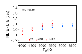
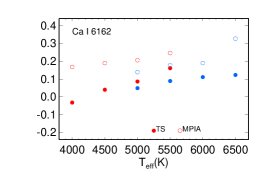
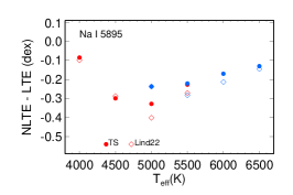
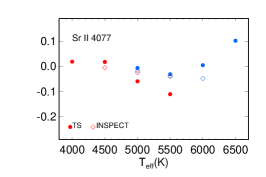
Figure 9: NLTE abundance corrections for Mg i 5528 Å, Ca i 6162 Å, Na i 5895 Å, and Sr ii 4077 Å depending on $T_{\rm eff}$ in the model atmospheres with [Fe/H] = $-3$ for two values of $\rm log~{}g$: 2.5 (red symbols) and 4.0 (blue symbols). The data taken from Lind et al. (2022) and the INSPECT database are shown by open diamonds and from the NLTE_MPIA database by open circles, while our calculations (TS) by filled circles.

4.2 Lines of Na i, Mg i, Ca i, Ca ii, and Sr ii

We selected Mg i 5528 Å, in order to compare our NLTE calculations with the 1D-NLTE corrections provided by the NLTE_MPIA database and by Lind et al. (2022, hereafter, Lind22). The used model atoms (from Bergemann et al., 2017, for NLTE_MPIA) are similar to ours, including a treatment of collisions with H i atoms. As seen in Fig. 9, our calculations agree very well with those of Lind22. The differences in $\Delta_{\rm NLTE}$ do not exceed 0.01 dex and 0.02 dex for the $\rm log~{}g$ = 4.0 and 2.5 models, respectively. The exception is the 4000/2.5/$-3$ model, for which we obtained a 0.065 dex more negative $\Delta_{\rm NLTE}$. NLTE_MPIA provides more positive NLTE corrections compared with ours, by 0.03–0.05 dex. The difference is 0.12 dex for the 4000/2.5/$-3$ model.

Similar model atoms of Na i were used in this study and by Lind22. The differences in $\Delta_{\rm NLTE}$ for Na i 5895 Å are very small ($\sim$0.01 dex) for the coolest and the hottest temperatures in Fig. 9. It is difficult to explain why TS – Lind22 = 0.07 dex for the 5000/2.5/$-3$ model, but TS – Lind22 = 0.00 for 5000/4.0/$-3$.

For lines of Sr ii, the 1D-NLTE corrections are provided by the INSPECT database. Their NLTE calculations were performed with the model atom developed by Bergemann et al. (2012b) and did not take into account collisions with H i atoms. This is in contrast to this study based on quantum-mechanical rate coefficients for the Sr ii + H i collisions. The atmospheric parameter range is narrower in INSPECT compared with this study, namely: 4400 K $\leq T_{\rm eff}\leq$ 6400 K, 2.2 $\leq\rm log~{}g\leq$ 4.6, $-3.9\leq$ [Fe/H] $\leq 0$. The differences in $\Delta_{\rm NLTE}$ for Sr ii 4077 Å are small except the models 5500/2.5/$-3$ and 6000/4.0/$-3$, where TS – INSPECT = $-0.07$ dex and +0.05 dex, respectively (Fig. 9).

The 1D-NLTE corrections for the Ca i lines at the NLTE_MPIA database were computed with the model atom developed by Mashonkina et al. (2007) and using Steenbock & Holweger (1984) formulas with $S_{\rm H}$ = 0.1 for calculating hydrogen collision rates. In this study, we applied the same model atom, however, the Ca i + H i collisions were treated using quantum-mechanical rate coefficients from Belyaev et al. (2017). As seen in Fig. 9, NLTE_MPIA provides systematically greater NLTE corrections for Ca i 6162 Å compared with our data, by 0.08 to 0.20 dex, probably due to a simplified treatment of hydrogenic collisions.

Ignoring the Ca ii + H i collisions in the SE calculations resulted in stronger NLTE effects for the Ca ii triplet lines in Merle et al. (2011) study compared with ours. For example, Merle et al. (2011) report the NLTE/LTE equivalent ratios of 1.28 and 1.16 for Ca ii 8498 and 8542 Å, respectively, in the 4250/1.5/$-4.0$ model, while our corresponding values are 1.22 and 1.12.

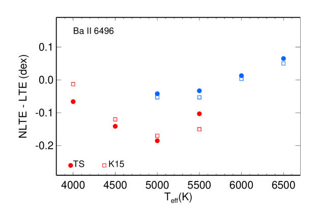
Figure 10: NLTE abundance corrections for Ba ii 6496 Å depending on $T_{\rm eff}$ in the model atmospheres with [Fe/H] = $-2$ for two values of $\rm log~{}g$: 2.5 (red symbols) and 4.0 (blue symbols). The filled circles and squares show our calculations (TS) and results of Korotin et al. (2015).

4.3 Lines of Ba ii

Finally, we compared our results with the 1D-NLTE corrections calculated by Korotin et al. (2015, K15) for lines of Ba ii. Korotin et al. (2015) provide the data for the $-2\leq$ [Fe/H] $\leq 0.5$ metallicity range. Therefore, $\Delta_{\rm NLTE}$ comparisons are presented in Fig. 10 for the same temperatures and surface gravities, as in Fig. 9, but for [Fe/H] = $-2$. The differences in $\Delta_{\rm NLTE}$ for Ba ii 6496 Å do not exceed 0.02 dex except the coolest and the hottest giant atmospheres, where TS – K15 = $-0.05$ dex and +0.05 dex, respectively.

To summarise this section, the situation with the 1D-NLTE corrections for lines of Na i, Mg i, and Fe i looks good. For each of these chemical species, there are, at least, two independent NLTE studies that predict consistent within 0.01-0.02 dex NLTE corrections and provide the grids which cover the full range of atmospheric parameters of VMP stars. For Sr ii and Ba ii, the NLTE corrections predicted by the independent studies agree reasonably well in the overlapping atmospheric parameter range.

5 Final remarks

This study presents grids of the 1D-NLTE abundance corrections for the Na i, Mg i, Ca i, Ca ii, Ti ii, Fe i, Zn i, Zn ii, Sr ii, and Ba ii lines, which are used in the galactic archaeology research. The range of atmospheric parameters represents VMP stars on various evolutionary stages and covers 4000 K $\leq T_{\rm eff}\ \leq$ 6500 K, 0.5 $\leq\rm log~{}g\ \leq$ 5.0, and $-5.0\leq$ [Fe/H] $\leq-2.0$. The NLTE corrections for Zn i, Zn ii, Sr ii, and Ba ii have been calculated for the first time for such a broad atmospheric parameter range. Compared to the data available in the literature, our NLTE corrections for lines of Ca i, Ca ii, Zn i, Zn ii, Sr ii, and Ba ii are based on accurate treatment of collisions with H i atoms in the statistical equilibrium calculations.

In the same model atmosphere, the NLTE abundance corrections may have different magnitude and sign for lines of the same chemical species, for example $\Delta_{\rm NLTE}$ = 0.092 dex (Mg i 5528 Å) and $\Delta_{\rm NLTE}=-0.083$ dex (Mg i 5172 Å) in the 4500/1.5/$-3.5$ model. Accounting for the NLTE effects in stellar abundance determinations is expected to improve an accuracy of the obtained results.

In the same model atmosphere, the NLTE abundance corrections may have different magnitude and sign for lines of different chemical species, for example, $\Delta_{\rm NLTE}$ = $-0.222$ dex (Na i 5895 Å) and $\Delta_{\rm NLTE}$ = 0.092 dex (Mg i 5528 Å) in the 4500/1.5/$-3.5$ model. Therefore, an appropriate treatment of the line formation is obligatory for the studies based on analysis of the stellar element abundance patterns.

For all spectral lines and chemical species, the NLTE corrections depend on metallicity. Neglecting the NLTE effects in stellar abundance determinations leads to distorted galactic abundance trends and incorrect conclusions on the Galactic chemical evolution.

We show that, for common spectral lines and the same atmospheric parameters, independent NLTE studies of Na i, Mg i, and Fe i predict consistent 1D-NLTE abundance corrections, with the difference of 0.01-0.02 dex in $\Delta_{\rm NLTE}$.

The obtained results are publicly available. At the website INASAN_NLTE (http://spectrum.inasan.ru/nLTE2/), we provide the tools for calculating online the NLTE abundance correction(s) for given line(s) and given atmospheric parameters.

6 Data availability

All our results are publicly available at the website INASAN_NLTE (http://spectrum.inasan.ru/nLTE2/).

References

- Ahumada et al. (2020) Ahumada R., et al., 2020, ApJS, 249, 3
- Alexeeva et al. (2014) Alexeeva S., Pakhomov Y., Mashonkina L., 2014, Astronomy Letters, 40, 406
- Amarsi & Asplund (2017) Amarsi A. M., Asplund M., 2017, MNRAS, 464, 264
- Amarsi et al. (2016a) Amarsi A. M., Asplund M., Collet R., Leenaarts J., 2016a, MNRAS, 455, 3735
- Amarsi et al. (2016b) Amarsi A. M., Lind K., Asplund M., Barklem P. S., Collet R., 2016b, MNRAS, 463, 1518
- Amarsi et al. (2018) Amarsi A. M., Barklem P. S., Asplund M., Collet R., Zatsarinny O., 2018, A&A, 616, A89
- Amarsi et al. (2019) Amarsi A. M., Barklem P. S., Collet R., Grevesse N., Asplund M., 2019, A&A, 624, A111
- Amarsi et al. (2020a) Amarsi A. M., Grevesse N., Grumer J., Asplund M., Barklem P. S., Collet R., 2020a, A&A, 636, A120
- Amarsi et al. (2020b) Amarsi A. M., et al., 2020b, A&A, 642, A62
- Amarsi et al. (2022) Amarsi A. M., Liljegren S., Nissen P. E., 2022, A&A, 668, A68
- Bailer-Jones (2015) Bailer-Jones C. A. L., 2015, PASP, 127, 994
- Barklem (2018) Barklem P. S., 2018, A&A, 612, A90
- Barklem et al. (2010) Barklem P. S., Belyaev A. K., Dickinson A. S., Gadéa F. X., 2010, A&A, 519, A20
- Barklem et al. (2012) Barklem P. S., Belyaev A. K., Spielfiedel A., Guitou M., Feautrier N., 2012, A&A, 541, A80
- Beers & Christlieb (2005) Beers T. C., Christlieb N., 2005, ARA&A, 43, 531
- Beers et al. (1985) Beers T. C., Preston G. W., Shectman S. A., 1985, AJ, 90, 2089
- Beers et al. (1992) Beers T. C., Preston G. W., Shectman S. A., 1992, AJ, 103, 1987
- Belyaev & Yakovleva (2018) Belyaev A. K., Yakovleva S. A., 2018, MNRAS, 478, 3952
- Belyaev et al. (2017) Belyaev A. K., Voronov Y. V., Yakovleva S. A., Mitrushchenkov A., Guitou M., Feautrier N., 2017, ApJ, 851, 59
- Belyaev et al. (2019) Belyaev A. K., Voronov Y. V., Yakovleva S. A., 2019, Phys. Rev. A, 100, 062710
- Bergemann et al. (2012a) Bergemann M., Lind K., Collet R., Magic Z., Asplund M., 2012a, MNRAS, 427, 27
- Bergemann et al. (2012b) Bergemann M., Hansen C. J., Bautista M., Ruchti G., 2012b, A&A, 546, A90
- Bergemann et al. (2017) Bergemann M., Collet R., Amarsi A. M., Kovalev M., Ruchti G., Magic Z., 2017, ApJ, 847, 15
- Bergemann et al. (2019) Bergemann M., et al., 2019, A&A, 631, A80
- Bessell et al. (1998) Bessell M. S., Castelli F., Plez B., 1998, A&A, 333, 231
- Bruls et al. (1992) Bruls J. H. M. J., Rutten R. J., Shchukina N. G., 1992, A&A, 265, 237
- Butler (1984) Butler K., 1984, Ph.D. Thesis, University of London
- Christlieb et al. (2002) Christlieb N., Wisotzki L., Graßhoff G., 2002, A&A, 391, 397
- Cohen et al. (2013) Cohen J. G., Christlieb N., Thompson I., McWilliam A., Shectman S., Reimers D., Wisotzki L., Kirby E., 2013, ApJ, 778, 56
- Dalton et al. (2014) Dalton G., et al., 2014, in Ramsay S. K., McLean I. S., Takami H., eds, Society of Photo-Optical Instrumentation Engineers (SPIE) Conference Series Vol. 9147, Ground-based and Airborne Instrumentation for Astronomy V. p. 91470L (arXiv:1412.0843), doi:10.1117/12.2055132
- Deng et al. (2012) Deng L.-C., et al., 2012, Research in Astronomy and Astrophysics, 12, 735
- Dotter et al. (2008) Dotter A., Chaboyer B., Jevremović D., Kostov V., Baron E., Ferguson J. W., 2008, ApJS, 178, 89
- Drawin (1969) Drawin H. W., 1969, Zeitschrift fur Physik, 225, 483
- Frebel & Norris (2015) Frebel A., Norris J. E., 2015, ARA&A, 53, 631
- Gaia Collaboration et al. (2016) Gaia Collaboration et al., 2016, A&A, 595, A2
- Gallagher et al. (2020) Gallagher A. J., Bergemann M., Collet R., Plez B., Leenaarts J., Carlsson M., Yakovleva S. A., Belyaev A. K., 2020, A&A, 634, A55
- Gerber et al. (2023) Gerber J. M., Magg E., Plez B., Bergemann M., Heiter U., Olander T., Hoppe R., 2023, A&A, 669, A43
- Giddings (1981) Giddings J., 1981, Ph.D. Thesis, University of London
- Gustafsson et al. (2008) Gustafsson B., Edvardsson B., Eriksson K., Jorgensen U. G., Nordlund Å., Plez B., 2008, A&A, 486, 951
- Kaulakys (1991) Kaulakys B., 1991, Journal of Physics B Atomic Molecular Physics, 24, L127
- Keller et al. (2007) Keller S. C., et al., 2007, Publ. Astron. Soc. Australia, 24, 1
- Kobayashi et al. (2020) Kobayashi C., Karakas A. I., Lugaro M., 2020, ApJ, 900, 179
- Korotin et al. (2015) Korotin S. A., Andrievsky S. M., Hansen C. J., Caffau E., Bonifacio P., Spite M., Spite F., François P., 2015, A&A, 581, A70
- Lind et al. (2017) Lind K., et al., 2017, MNRAS, 468, 4311
- Lind et al. (2022) Lind K., et al., 2022, A&A, 665, A33
- Lindegren et al. (2021) Lindegren L., et al., 2021, A&A, 649, A4
- Majewski et al. (2017) Majewski S. R., et al., 2017, AJ, 154, 94
- Mashonkina (2013) Mashonkina L., 2013, A&A, 550, A28
- Mashonkina & Belyaev (2019) Mashonkina L. I., Belyaev A. K., 2019, Astronomy Letters, 45, 341