Abstract

In a time-harmonic setting, we show for heterogeneous acoustic and homogeneous electromagnetic wavesguides stability estimates with the stability constant depending linearly on the length $L$ of the waveguide. These stability estimates are used for the analysis of the (ideal) ultraweak (UW) variant of the Discontinuous Petrov Galerkin (DPG) method. For this UW DPG, we show that the stability deterioration with $L$ can be countered by suitably scaling the test norm of the method. We present the “full envelope approximation”, a UW DPG method based on non-polynomial ansatz functions that allows for treating long waveguides.

1 Introduction

Motivation.

Acoustic and electromagnetic (EM) waveguide problems have many important applications and are therefore discussed widely in the literature [26, 39, 1, 15, 23]. For many applications of interest, such as optical fibers, the propagating wave has high frequency and the waveguide length, denoted by $L$ throughout this work, is very large compared to the wavelength. It is therefore challenging to approximate the solution numerically; to obtain an accurate solution, one must sufficiently resolve the wavelength scale and additionally counter the effect of numerical pollution to overcome stability issues of the discretization [2, 10].

While the stability of Finite Element (FE) discretizations of Helmholtz and time-harmonic Maxwell problems has been analyzed in fixed domains for increasing wave frequency $\omega$ [33, 6, 34], there is to the best of our knowledge no such corresponding analysis for the waveguide problem where $\omega$ is fixed and the waveguide length $L$ increases. In practical applications, this is of great relevance as the available computational tools become more powerful thereby enabling numerical solution of waveguide models of realistic length scales. We discuss the present work in the context of modeling optical fiber amplifiers but emphasize that the main results of this work are relevant to FE discretization of acoustic and EM waveguide problems with the Discontinuous Petrov–Galerkin (DPG) Method [5] in general.

Optical amplifiers.

Optical fiber amplifiers can produce highly coherent laser outputs with great efficiency, which has enabled advances in many engineering applications [24]. However, at high-power operation, these fiber laser systems are susceptible to the onset of various nonlinear effects that are adverse to the beam quality of the laser [1, 27, 38]. One particular challenge is mitigating the effects of heating of the silica-glass fiber. Under sufficient heat load, the fiber amplifier experiences a thermally-induced nonlinear effect called the transverse mode instability (TMI) [9, 25]. TMI is characterized by a sudden reduction of the beam coherence above a certain power threshold. This instability is a major limitation for the average power scaling of fiber laser systems [25]. While a scientific consensus on the thermal origins of TMI has developed over the past years, finding effective mitigation strategies that do not incite other power limiting nonlinearities remains an active field of research in fiber optics.

In the context of studying TMI and other nonlinear effects in fibers, numerical simulations play an important role. Typically, a model needs to account for two fields in the fiber amplifier: 1) the signal laser, a highly coherent light source that is seeded into the fiber core; and 2) the pump field, which provides the energy for amplification of the signal and is typically injected into the fiber cladding. A variety of different models are employed in fiber amplifier simulations (e.g., [37, 40, 35, 14] and references therein). These models are usually derived from the time-harmonic Maxwell equations, and by making additional modeling assumptions they become easier to discretize and compute than a vectorial Maxwell problem.

Vectorial Maxwell fiber amplifier model.

This work is part of a continued effort to build reliable, high-fidelity FE models for investigating TMI in optical amplifiers [36, 16, 17, 19, 18]. The model consists of a system of two nonlinear time-harmonic Maxwell equations (one for the signal field and one for the pump field) coupled with each other and with the transient heat equation to account for thermal effects [36, 17]. Modeling of a 1–10 m long fiber segment involves the solution with $\mathcal{O}$(1–10 M) wavelengths. Solving such a problem with a direct FE discretization is infeasible, even on state-of-the-art supercomputers. Hence, our initial efforts focused on so-called equivalent short fiber models, which artificially scale physical parameters of the model, involving first $\mathcal{O}$(100) wavelengths (using OpenMP parallelization) [36, 17], and then, more realistic models of (a tiny segment of) the actual fiber with up to $\mathcal{O}$(10,000) wavelengths [16, 19, 18] (using MPI+OpenMP parallelization and up to 512 manycore compute nodes).

Because the laser light in a meter-long optical fiber has millions of wavelengths, it is extremely difficult to resolve the wavelength scale of the propagating light for the full length. For this reason, even simplified models typically resolve a longer length scale. In the context of TMI studies, it is common to resolve only the length scale of the mode beat between the fundamental mode and higher-order modes since the mode instabilities occur at that scale. In a typical weakly-guiding, large-mode-area fiber amplifier, the mode beat length is on order of $\mathcal{O}$(1,000) wavelengths.

This brought forth the idea of the full envelope approximation, the solution to an alternative formulation of our vectorial Maxwell model in which the field is less oscillatory in the (longitudinal) $z$-direction. Consider the linear time-harmonic Maxwell equations in a non-magnetic and dielectric medium, in the absence of free charges:

$$\bm{\nabla}\times\bm{E} =-i\omega\mu_{0}\bm{H}\,,$$ (1.1)

$$\bm{\nabla}\times\bm{H} =i\omega{\epsilon}\bm{E}\,,$$ (1.2)

where $i=\sqrt{-1}$, $\omega$ is the angular frequency of the light, $\mu_{0}$ denotes permeability in vacuum, and ${\epsilon}={\epsilon}(x,y,z)$ denotes permittivity. The idea of the full envelope approximation is very simple: Instead of solving for the original EM field $(\bm{E},\bm{H})$ using (1.1)–(1.2), we seek the solution in the form:

$$\bm{E}(x,y,z) =\bm{\mathsf{E}}(x,y,z)e^{-ikz}\,,$$ (1.3)

$$\bm{H}(x,y,z) =\bm{\mathsf{H}}(x,y,z)e^{-ikz}\,,$$ (1.4)

where the envelope wavenumber $k$ corresponds to a dominant frequency in the waveguide $z$-direction. If the effective wavenumber of the propagating fields $(\bm{E},\bm{H})$ in the $z$-direction is indeed close to $k$, then the approximation of the new fields ($\bm{\mathsf{E}}$, $\bm{\mathsf{H}}$) requires orders of magnitude fewer elements along the fiber than the approximation of the original fields $(\bm{E},\bm{H})$. Upon substituting the ansatz into Maxwell’s equations and factoring out the exponential, we obtain the modified Maxwell model

$$\bm{\nabla}\times\bm{\mathsf{E}}-ik\bm{e}_{z}\times\bm{\mathsf{E}} =-i\omega\mu_{0}\bm{\mathsf{H}}\,,$$ (1.5a)

$$\bm{\nabla}\times\bm{\mathsf{H}}-ik\bm{e}_{z}\times\bm{\mathsf{H}} =i\omega{\epsilon}\bm{\mathsf{E}}\,,$$ (1.5b)

where $\bm{e}_{z}=(0,0,1)^{T}$ is the unit vector in $z$-direction. This idea has turned out to be very successful enabling modeling of TMI in fiber amplifiers with several million wavelengths [20].

Scope of this work.

The presented paper provides theoretical foundations for the full envelope model and the convergence of the ultraweak DPG method for acoustic and EM waveguide problems with increasing waveguide length $L$. Numerical studies to this extent were carried out in [16]; however, the convergence of the method was not analyzed therein.

We begin by introducing in Section 2 two model problems of interest: a (possibly non-homogeneous) acoustic waveguide, and a homogeneous EM waveguide. In the same section, we provide a quick overview of DPG analysis and demonstrate that the modified Maxwell model resulting from the full envelope ansatz shares the boundedness below constant with the original Maxwell operator. Section 3 analyses the Helmholtz problem (main result: Theorem 3.5), and Section 4 analyses the Maxwell problem (main result: Theorem 4.5). Section 5 presents numerical results and concludes with a discussion on the non-homogeneous EM waveguide problem.

Notation.

We use $(\cdot,\cdot)_{L^{2}}$ and $\|\cdot\|_{L^{2}}$ to denote the standard sesquilinear form (antilinear in the second argument) and associated norm on the Hilbert space $L^{2}$. If clear from the context, we write $(\cdot,\cdot)$ and $\|\cdot\|$ respectively. For Sobolev spaces on Lipschitz domains $\omega\subset\mathbb{R}^{d}$, we follow the conventions of [29], i.e., for $s\geq 0$ we denote by $H^{s}(\omega)$ the closure of $C^{\infty}(\overline{\omega})$ under the norm $\|\cdot\|_{H^{s}(\omega)}$, $\widetilde{H}^{s}(\omega)$ is the closure of $C^{\infty}_{0}(\omega)$ under the norm $\|\cdot\|_{H^{s}(\mathbb{R}^{d}})$, $H^{-s}(\omega)$ is the dual of $\widetilde{H}^{s}(\omega)$ and $\widetilde{H}^{-s}(\omega)$ the dual of $H^{s}(\omega)$. The constant $C>0$ may be different in each occurance but does not depend on critical parameters such as the length $L$ of the waveguide. The expression $A\lesssim B$ indicates the existence of $C>0$ such that $A\leq CB$ with the implied constant $C$ independent of critical parameters.

2 Model problems and DPG formulation

We present two model problems whose stability we analyze in the following sections. Throughout this work, $D\subset\mathbb{R}^{d}$, $d\in\mathbb{N}$, is a bounded Lipschitz domain with a piecewise smooth boundary, $L>0$, and we set $\Omega=D\times(0,L)$. Throughout, we assume ${\omega}>0$ given.

2.1 Helmholtz problem

On $D$ let $a:D\rightarrow\operatorname{GL}({\mathbb{R}}^{d\times d})$ be a pointwise symmetric positive definite matrix with $0<\lambda_{min}\leq a\leq\lambda_{max}<\infty$ uniformly in $x\in D$. Set

$$\mathfrak{a}:=\left(\begin{array}[]{cc}a(x)&0\\ 0&1\end{array}\right).$$

On ${\Omega}=D\times(0,L)\subset\mathbb{R}^{d+1}$ we consider

$$i{\omega}\bm{u}+\mathfrak{a}\nabla p =f\quad\mbox{in ${\Omega}$},$$ (2.1a)

$$i{\omega}p+\operatorname{div}\bm{u} =\bm{g}\quad\mbox{in ${\Omega}$},$$ (2.1b)

$$p =0\quad\mbox{on $\Gamma_{\text{in}}:=D\times\{0\}$},$$ (2.1c)

$$\bm{u}\cdot\bm{n} =0\quad\mbox{on $\Gamma_{\text{lat}}:=\partial D\times\{0,L\}$},$$ (2.1d)

$$i{\omega}\bm{u}\cdot\bm{n}-\operatorname{DtN}p =0\quad\mbox{on $\Gamma_{\text{out}}:=D\times\{L\}$}.$$ (2.1e)

Here, $\bm{n}$ denotes the outer normal vector on $\partial\Omega$. We describe the operator $\operatorname{DtN}$ in (3.8) in Section 3.2. This operator ensures that waves are “outgoing” on $\Gamma_{\text{out}}$. That is, if one considers instead an infinite waveguide $D\times(0,\infty)$ such that the right-hand sides $f$, $\bm{g}$ vanish on $D\times(L,\infty)$, one requires that waves be going to the right.

We define the operator

$$A^{\operatorname*{helm}}\left(\begin{array}[]{c}p\\ \bm{u}\end{array}\right):=\left(\begin{array}[]{c}i{\omega}\bm{u}+\mathfrak{a}\nabla p\\ i{\omega}p+\operatorname{div}\bm{u}\end{array}\right)$$ (2.2)

with domain $D(A^{\operatorname*{helm}})$ that includes the boundary conditions and is given by

$$\begin{split}D(A^{\operatorname*{helm}})=\{(p,\bm{u})\in H^{1}(\Omega)\times\bm{H}({\rm div},\Omega)\,|\,&\ p|_{\Gamma_{\text{in}}}=0,\ \bm{u}\cdot\bm{n}=0\mbox{ in $H^{-1/2}(\Gamma_{\text{lat}})$},\\ &\ i{\omega}\bm{u}\cdot\bm{n}-\operatorname{DtN}p=0\mbox{ in $\widetilde{H}^{-1/2}(\Gamma_{\text{out}})$}\}.\end{split}$$ (2.3)

2.2 Maxwell problem

Let $d=2$. In a homogeneous medium, we consider the Maxwell system for the electric field $\bm{E}$ and the magnetic field $\bm{H}$ that satisfy

$$\bm{\nabla}\times\bm{E}-i\omega\bm{H} =\bm{f}\ \mbox{in $\Omega=D\times(0,L)\subset\mathbb{R}^{3}$},$$ (2.4a)

$$\bm{\nabla}\times\bm{H}+i\omega\bm{E} =\bm{g}\ \mbox{in $\Omega\subset\mathbb{R}^{3}$},$$ (2.4b)

$$\gamma_{t}\bm{E} =0\ \mbox{on $\Gamma_{\text{in}}$},$$ (2.4c)

$$\gamma_{t}\bm{E} =0\ \mbox{on $\Gamma_{\text{lat}}$},$$ (2.4d)

$$\pi_{t}\bm{H}-\operatorname{DtN}^{\operatorname{mw}}\bm{E} =0 \mbox{ on $\Gamma_{\text{out}}$}.$$ (2.4e)

Here, $\gamma_{t}\bm{E}=\bm{E}\times\bm{n}$ is the tangential trace on $\partial\Omega$, $\pi_{t}\bm{H}=\bm{n}\times(\bm{H}\times\bm{n})$ the tangential component, and the operator $\operatorname{DtN}^{\operatorname{mw}}$ is described in Section 4 in (4.22) and realizes that waves are “outgoing” at $z=L$.

Problem (2.4) can be written in operator form

$$A^{\operatorname*{maxwell}}\left(\begin{array}[]{c}\bm{E}\\ \bm{H}\end{array}\right)=\left(\begin{array}[]{c}\bm{f}\\ \bm{g}\end{array}\right)\,,\qquad A^{\operatorname*{maxwell}}\left(\begin{array}[]{c}\bm{E}\\ \bm{H}\end{array}\right):=\left(\begin{array}[]{c}\nabla\times\bm{E}-i{\omega}\bf H\\ \nabla\times\bm{H}+i{\omega}\bm{E}\end{array}\right),$$ (2.5)

where the domain $D(A^{\operatorname*{maxwell}})$ includes the boundary conditions and is given by

$$D(A^{\operatorname*{maxwell}}) =\{(\bm{E},\bm{H})\in\bm{H}_{0,\Gamma_{-}}(\operatorname{curl},{\Omega})\times\bm{H}(\operatorname{curl},{\Omega})\,|\,\pi_{t}\bm{H}=\operatorname{DtN}^{\operatorname{mw}}\bm{E}\mbox{ on $\Gamma_{\text{out}}$}\},$$ (2.6)

with $\Gamma_{-}:=\partial{\Omega}\setminus\overline{\Gamma_{\text{out}}}$ and

$$\bm{H}_{0,\Gamma_{-}}=\{\bm{E}\in\bm{H}(\operatorname{curl},{\Omega})\,|\,\gamma_{t}\bm{E}=0\quad\mbox{ on $\Gamma_{-}$}\}.$$ (2.7)

2.3 Ultraweak DPG formulation and DPG essentials

Suppose we are given an injective closed operator representing a system of first-order linear Partial Differential Equations (PDEs),

$$A\,:\,L^{2}(\Omega)\supset D(A)\to L^{2}(\Omega)\,,$$

where $D(A)$ is the domain of the operator incorporating (homogeneous) Boundary Conditions (BCs). We want to solve the problem,

$$\left\{\begin{array}[]{lll}u\in D(A)\\[5.0pt] Au=f\,.\end{array}\right.$$

The problem is trivially equivalent to the so-called strong variational formulation:

$$\left\{\begin{array}[]{lll}u\in H_{A}(\Omega)\\[5.0pt] (Au,v)=(f,v)\quad\forall\,v\in L^{2}(\Omega)\,,\end{array}\right.$$

where $H_{A}(\Omega):=D(A)$ is a Hilbert space equipped with the graph norm:

$$\|u\|^{2}_{H_{A}}:=\|u\|^{2}+\|Au\|^{2}\,.$$

The ultraweak (UW) variational formulation is obtained by integrating by parts and passing all derivatives to the test function. It reads as follows:

$$\left\{\begin{array}[]{lll}u\in L^{2}(\Omega)\\[5.0pt] (u,A^{\ast}v)=(f,v)\quad\forall\,v\in H_{A^{\ast}}(\Omega)\,,\end{array}\right.$$ (2.8)

where

$$A^{\ast}\,:\,L^{2}(\Omega)\supset D(A^{\ast})\to L^{2}(\Omega)$$

is the $L^{2}$-adjoint of the original operator in the sense of closed operator theory, assumed to be injective as well, and the test space $H_{A^{\ast}}(\Omega):=D(A^{\ast})$ has been equipped with the scaled adjoint graph norm:

$$\|v\|^{2}_{H_{A^{\ast}}}:=\beta^{2}\|v\|^{2}+\|A^{\ast}v\|^{2}$$

with $\beta\geq 0$. As the test functions are now more regular (and the solution less regular), the right-hand side may be upgraded to an arbitrary continuous and antilinear functional $l(\cdot)$ on $H_{A^{\ast}}(\Omega)$.

Lemma 2.1

Assume that that the operator $A$ is bounded below with a (boundedness below) constant $\alpha>0$:

$$\alpha\|u\|\leq\|Au\|\qquad\forall u\in D(A)\,.$$

The UW formulation (2.8) is then well-posed with the inf-sup constant

$$\gamma\geq\left[1+\left(\frac{\beta}{\alpha}\right)^{2}\right]^{-\frac{1}{2}}\,.$$

Proof:     The Closed Range Theorem implies that adjoint $A^{\ast}$ is bounded below with the same constant $\alpha$. Take an arbitrary $u\in L^{2}(\Omega)$ and consider the corresponding solution $v_{u}$ of the adjoint problem,

$$\left\{\begin{array}[]{ll}v_{u}\in D(A^{\ast})\\[5.0pt] A^{\ast}v_{u}=u\,.\end{array}\right.$$

We have:

$$\|v_{u}\|\leq\alpha^{-1}\|u\|\quad\Rightarrow\quad\|v_{u}\|_{H_{A^{\ast}}}^{2}=\|A^{\ast}v\|^{2}+\beta^{2}\|v\|^{2}\leq\left[1+\left(\frac{\beta}{\alpha}\right)^{2}\right]\|u\|^{2}\,,$$

and, in turn,

$$\sup_{v\in D(A^{\ast})}\frac{|(u,A^{\ast}v)|}{\|v\|_{A^{\ast}}}\geq\frac{|(u,u)|}{\|v_{u}\|_{A^{\ast}}}\geq[1+\left(\frac{\beta}{\alpha}\right)^{2}]^{-\frac{1}{2}}\frac{|(u,u)|}{\|u\|}=\left[1+\left(\frac{\beta}{\alpha}\right)^{2}\right]^{-\frac{1}{2}}\|u\|\,.$$

Finally, the conjugate operator coincides with the strong operator $A$ and its injectivity implies the existence of the solution for any right-hand side $l\in H_{A^{\ast}}(\Omega)^{\prime}$.       

Note that, for $\beta=0$, the inf-sup constant is one. The DPG Method with Optimal Test Functions is based on extending the UW formulation to a larger class of broken test functions $H_{A^{\ast}}(\Omega_{h})$ [4]. Unfortunately, for $\beta=0$, the form $b(u,v)=(u,A^{\ast}v)$ is not localizable, i.e. the adjoint test norm cannot be extended to the broken test space and we must use a positive scaling constant $\beta>0$. In principle though, by employing a sufficiently small constant $\beta$, we can make the inf-sup constant as close to one as we wish. It is not intuitive at all that the UW formulation allows for improving the stability of the original operator $A$ in the strong setting.

Finally, the stability of the UW formulation is inherited by the broken formulation [4]. In the ideal DPG method, the optimal test functions are assumed to be computed exactly; the discrete inf-sup constant is bounded from below by the continuous inf-sup constant which indicates the relevance of understanding the continuous variational problem. The ideal DPG method is merely a logical construct on the way to analyze the practical DPG method where the optimal test functions are computed approximately. The additional error resulting from the approximation of the test functions is analyzed with the help of appropriate Fortin operators [5].

2.4 The full envelope approximation (1.5)

The analysis of the stability of the full envelope approximation method (1.5) turns out to be surprisingly simple.

Lemma 2.2

Let $\widetilde{A}$ be the operator corresponding to the full envelope ansatz, i.e.,

$$\widetilde{A}\widetilde{u}:=e^{ikz}A(e^{-ikz}\widetilde{u})\,,$$

where $A\in\{A^{\operatorname*{helm}},A^{\operatorname*{maxwell}}\}$ denotes the operator corresponding to the acoustic or EM waveguide problem. Then, the operator $\widetilde{A}$ is bounded below if and only if operator $A$ is bounded below, and the corresponding boundedness below constants are identical:

$$\|Au\|\geq\alpha\|u\|\quad\Leftrightarrow\quad\|\widetilde{A}\widetilde{u}\|\geq\alpha\|\widetilde{u}\|\,.$$

Proof:     We observe

$$\|\widetilde{A}\widetilde{u}\|=\|e^{ikz}A(e^{-ikz}\widetilde{u})\|=\|A(e^{-ikz}\widetilde{u})\|\geq\alpha\|e^{-ikz}\widetilde{u}\|=\alpha\|\widetilde{u}\|\,.$$

 

3 Stability

Section 2.3 shows that at the heart of the analysis of the ultraweak DPG method is the understanding of the stability properties of the operator $A$. In this section, we provide the stability of operator $A^{\operatorname*{helm}}$ of the Helmholtz problem (2.1) making the dependence on the length $L$ of the waveguide explicit. In view of Lemma 2.1, this analysis then provides a guideline for selecting the parameter $\beta$ in the DPG method.

3.1 Analysis of the 1D Helmholtz equation

Since the domain $\Omega=D\times(0,L)$ has product structure and the coefficients of the Helmholtz equation are independent of the longitudinal variable, a decoupling into transversal modes is possible and leads to a stability analysis analysis of 1D equations. In the present section, we present the necessary 1D stability results.

Lemma 3.1 ([32, Thm. 4.3])

Let $\hat{I}:=(0,1)$. Let $\hat{\kappa}\in\mathbb{C}_{\geq 0}:=\{z\in\mathbb{C}\colon\operatorname*{Re}\geq 0\}$ satisfy $|\hat{\kappa}|\geq 1$. Introduce $H^{1}_{(0}(\hat{I}):=\{u\in H^{1}(\hat{I})\colon u(0)=0\}$ and the sesquilinear form

$$a^{1D}_{\hat{\kappa},\hat{I}}(u,v):=(u^{\prime},v^{\prime})_{L^{2}(0,1)}+\hat{\kappa}^{2}(u,v)_{L^{2}(0,1)}+\hat{\kappa}u(1)\overline{v}(1).$$

Introduce on $H^{1}(\hat{I})$ the norm $\|\cdot\|_{1,|\kappa|,\hat{I}}$ by $\|u\|^{2}_{1,|\hat{\kappa}|}:=\|u^{\prime}\|^{2}_{L^{2}(\hat{I})}+|\hat{\kappa}|^{2}\|u\|^{2}_{L^{2}(\hat{I})}$. Then there is $c>0$ independent of $\kappa$ such that for both choices $V=H^{1}(\hat{I})$ and $V=H^{1}_{(0}(\hat{I})$ there holds

$$\hat{\gamma}_{\hat{\kappa}}:=\inf_{0\neq u\in V}\sup_{0\neq V}\frac{\operatorname*{Re}a^{1D}_{\hat{\kappa},\hat{I}}(u,v)}{\|u\|_{1,|\hat{\kappa}|,\hat{I}}\|v\|_{1,|\hat{\kappa}|,\hat{I}}}\geq\frac{1}{1+c\frac{\operatorname*{Im}\hat{\kappa}}{1+\operatorname*{Re}\hat{\kappa}}}$$ (3.1)

Proof:     The proof follows essentially from [32, Thm. 4.3], where a similar sesquilinear form in 2D and 3D is considered. Details are given in Appendix A.       

It is convenient to introduce for $\kappa\in\mathbb{C}$ and an interval $I=(0,L)$ the sesquilinear form $a^{1D}_{\kappa}$ and the norm $\|\cdot\||_{1,|\kappa|}$ by

$$a^{1D}_{\kappa}(u,v) :=(u^{\prime},v^{\prime})_{L^{2}(I)}+\kappa^{2}(u,v)_{L^{2}(I)}+\kappa u(L)\overline{v}(L),$$ (3.2)

$$\|q\|^{2}_{1,|\kappa|} :=\|q^{\prime}\|^{2}_{L^{2}(I)}+|\kappa|^{2}\|q\|^{2}_{L^{2}(I)}\,.$$ (3.3)

Lemma 3.2

Let $I=(0,L)$ and $V=H^{1}(I)$ or $V=H^{1}_{(0}(I):=\{w\in H^{1}(I)\colon w(0)=0\}$. Let $\kappa\in\mathbb{C}_{\geq 0}$ with $|\kappa|\geq 1$. Consider the following two problems: Find $q_{1}$, $q_{2}\in V$ such that

$$a^{1D}_{\kappa}(q_{1},w) =(f,w)_{L^{2}(I)} \quad\forall w\in V\,,$$

$$a^{1D}_{\kappa}(q_{1},w) =(f,w^{\prime})_{L^{2}(I)} \quad\forall w\in V\,.$$

Then the following holds:

1. There are $C$, $c>0$ depending only on a lower bound for $L|\kappa|$ such that with

   $$\gamma:=\frac{1}{1+c\frac{|\operatorname*{Im}(L\kappa)|}{1+\operatorname*{Re}(L\kappa)}}$$ (3.4)

   there holds

   $$\|q_{1}\|_{1,|\kappa|} \leq C\frac{L}{\gamma|\kappa|}\|f\|_{L^{2}(I)}\,, \|q_{2}\|_{1,|\kappa|} \leq C\gamma^{-1}\|f\|_{L^{2}(I)}\,.$$

2. If $\kappa\in i\mathbb{R}$, then we have for a constant $C>0$ depending only on a lower bound for $L|\kappa|$

   $$\|q_{1}\|_{1,|\kappa|} \leq CL\|f\|_{L^{2}(I)}\,, \|q_{2}\|_{1,|\kappa|} \leq CL|\kappa|\|f\|_{L^{2}(I)}\,,$$

3. If $\kappa>0$, then we have for a constant $C>0$ depending only on a lower bound for $L\kappa$

   $$\|q_{1}\|_{1,\kappa} \leq C\kappa^{-1}\|f\|_{L^{2}(I)}\,, \|q_{2}\|_{1,\kappa} \leq C\|f\|_{L^{2}(I)}\,.$$

Proof:     Rescaling the equation posed on $(0,L)$ to an equation posed on $(0,1)=:\hat{I}$, we get by denoting the rescaled functions with a $\hat{\cdot}$ and $\hat{\kappa}:=L\kappa$ and spaces $\hat{V}=H^{1}(\hat{I})$ if $V=H^{1}(I)$ and $\hat{V}=H^{1}_{(0}(\hat{I})$ if $V=H^{1}_{(0}(I)$

$$(\hat{q}^{\prime}_{1},w^{\prime})_{L^{2}(0,1)}+\hat{\kappa}^{2}(\hat{q}_{1},w)_{L^{2}(0,1)}+\hat{\kappa}\hat{q}_{1}(1)\overline{w(1)} =L^{2}(\hat{f},w)_{L^{2}(I)}\quad\forall w\in\hat{V},$$

$$(\hat{q}^{\prime}_{2},w^{\prime})_{L^{2}(I)}+\hat{\kappa}^{2}(\hat{q}_{2},w)_{L^{2}(I)}+\hat{\kappa}\hat{q}_{2}(1)\overline{w(1)} =L(\hat{f},w^{\prime})_{L^{2}(I)}\quad\forall w\in\hat{V}.$$

In terms of the inf-sup constant $\hat{\gamma}_{\hat{\kappa}}$ of (3.1), i.e.,

$$\gamma:=\inf_{q\in\hat{V}}\sup_{w\in\hat{V}}\frac{|a^{1D}_{\hat{\kappa}}(q,w)|}{\|q\|_{1,|\hat{\kappa}|}\|w\|_{1,|\hat{\kappa}|}}$$

we have

$$\|\hat{q}_{1}\|_{1,|\hat{\kappa}|} \leq C\gamma^{-1}|\hat{\kappa}|^{-1}\|L^{2}\hat{f}\|_{L^{2}(\hat{I})},$$

$$\|\hat{q}_{2}\|_{1,|\hat{\kappa}|} \leq C\gamma^{-1}\|L\hat{f}\|_{L^{2}(\hat{I})}$$

with $C>0$ depending only on a lower bound for $|\hat{\kappa}|$. Scaling back to $(0,L)$ yields

$$\|q_{1}\|_{1,|\kappa|} \sim L^{-1/2}\|\hat{q}_{1}\|_{1,|\hat{\kappa}|}\leq CL^{2}L^{-1/2}\gamma^{-1}|\hat{\kappa}|^{-1}\|\hat{f}\|_{L^{2}(\hat{I})}\leq CL\gamma^{-1}|\hat{\kappa}|^{-1}\|f\|_{L^{2}(I)},$$

$$\|q_{2}\|_{1,|\kappa|} \sim L^{-1/2}\|\hat{q}_{2}\|_{1,|\hat{\kappa}|}\leq CL^{1/2}\gamma^{-1}\|\hat{f}\|_{L^{2}(\hat{I})}\leq C\gamma^{-1}\|f\|_{L^{2}(I)}.$$

Proof of (i): By Lemma 3.1, $\gamma$ has the form (3.4). The result follows.

Proof of (ii): For $\kappa\in i\mathbb{R}$, the inf-sup constant $\gamma$ of (3.4) satisfies $\gamma\sim|\hat{\kappa}|^{-1}$ with a implied constants depending on a lower bound for $|\hat{\kappa}|$. The result follows.

Proof of (iii): For $\kappa>0$, the inf-sup constant $\gamma$ of (3.4) satisfies $\gamma\sim 1$ with implied constants depending only on a lower bound for $|\hat{\kappa}|$. The result follows.       

3.2 The $\operatorname{DtN}$ operator

We describe the $\operatorname{DtN}$-operator at the outflow boundary $\Gamma_{\text{out}}$. This is achieved in terms of a modal decomposition obtained by a suitable eigenvalue problem in transverse direction.

Let $(\varphi_{n},\lambda_{n})_{n\in\mathbb{N}}\subset H^{1}(D)\setminus\{0\}\times\mathbb{R}^{+}$ be the eigenpairs of the operator $p\mapsto-\operatorname{div}(a\nabla u)$, i.e.,

$$-\operatorname{div}(a\nabla\varphi_{n}) =\lambda_{n}\varphi_{n}\quad \mbox{in $D$},$$ (3.5a)

$$\bm{n}\cdot a\nabla\varphi_{n} =0\quad \partial D$$ on (3.5b)

with the normalization $\|\varphi_{n}\|_{L^{2}(D)}=1$ for all $n\in\mathbb{N}$. Here, the normal vector $\bm{n}$ is the outer normal on $\partial D$. We have the orthogonalities

$$(\varphi_{n},\varphi_{m})_{L^{2}(D)}=\delta_{nm},\qquad(a\nabla\varphi_{n},\nabla\varphi_{m})_{L^{2}(D)}=\delta_{nm}\lambda_{n}.$$ (3.6)

The positive values $\lambda_{n}$ are assumed sorted in ascending order and listed according to their multiplicity. We collect them in the spectrum $\sigma=\{\lambda_{n}\colon n\in\mathbb{N}\}$. It is convenient to derive the operator $\operatorname{DtN}$ in (2.1d) using the second-order formulation for $(f,\bm{g})=(0,0)$, i.e., consider

$$-\operatorname{div}(\mathfrak{a}\nabla p)-{\omega}^{2}p =0\quad\mbox{ on $D\times(L,\infty).$}$$

Making the ansatz $p(x,z)=\sum_{n}p_{n}(z)\varphi_{n}(x)$ yields the 1D equations

$$-p_{n}^{\prime\prime}(z)+(\lambda_{n}-{\omega}^{2})p_{n} =0\quad\mbox{ on $(L,\infty)$}$$

with the fundamental solutions $e^{\pm\kappa_{n}z}$, where

$$\kappa_{n}:=\sqrt{\lambda_{n}-{\omega}^{2}}$$ (3.7)

and the square root is taken to be the principal branch. Writing $p|_{\Gamma_{\text{out}}}=\sum_{n}p_{n}(L)\varphi_{n}(x)$, the “outgoing” solution is defined on $(L,\infty)$ to be

$$p(x,z)=\sum_{n}p_{n}(L)\varphi_{n}(x)e^{-\kappa_{n}(z-L)}.$$

The operator $\operatorname{DtN}$ is given by $p|_{\Gamma_{\text{out}}}\mapsto(\partial_{z}p(x,z))|_{z=L}$, viz.,

$$\operatorname{DtN}p :=-\sum_{n}p_{n}\kappa_{n}\varphi_{n}(x),\qquad p_{n}:=(p,\varphi_{n})_{L^{2}(D)}.$$ (3.8)

The indices $n\in\mathbb{N}$ with $\kappa_{n}>0$ are called evanescent modes, those with $\kappa_{n}\in i\mathbb{R}\setminus\{0\}$ are the propagating modes. We assume throughout that

$$\kappa_{n}\neq 0\qquad\forall n\in\mathbb{N}$$ (3.9)

so that we can write $\mathbb{N}=I_{\text{prop}}\dot{\cup}I_{\text{eva}}$ with the finite set $I_{\text{prop}}$ of propagating modes and the infinite set $I_{\text{eva}}$ of evanescent modes:

$$I_{\text{prop}}:=\{n\in\mathbb{N}\,|\,\kappa_{n}\in i\mathbb{R}\},\qquad I_{\text{eva}}:=\{n\in\mathbb{N}\,|\,\kappa_{n}>0\}.$$ (3.10)

Concerning the mapping properties of $\operatorname{DtN}$, we have

$$\operatorname{DtN}:H^{1/2}(\Gamma_{\text{out}})\rightarrow\widetilde{H}^{-1/2}(\Gamma_{\text{out}}):=(H^{1/2}(\Gamma_{\text{out}}))^{\prime}$$

is bounded, linear, which follows from the representation of $\operatorname{DtN}$: Since $H^{1/2}(\Gamma_{\text{out}})$ is the interpolation space between $L^{2}(\Gamma_{\text{out}})$ and $H^{1}(\Gamma_{\text{out}})$ (see, e.g., [29]), we we have the norm equivalence $\|p\|^{2}_{H^{1/2}(\Gamma_{\text{out}})}\sim\sum_{n}|p_{n}|^{2}\sqrt{\lambda_{n}}$, where $p=\sum_{n}p_{n}\varphi_{n}$ with $p_{n}=(p,\varphi_{n})_{L^{2}(D)}$. Hence, writing $p$, $q\in H^{1/2}(\Gamma_{\text{out}})$ in the form $p=\sum_{n}p_{n}\varphi_{n}$ and $q=\sum_{n}q_{n}\varphi_{n}$, we estimate

$$\left|\langle\operatorname{DtN}p,q\rangle\right| =\left|-\sum_{n}\kappa_{n}p_{n}\overline{q}_{n}\right|\lesssim\|p\|_{H^{1/2}(\Gamma_{\text{out}})}\|q\|_{H^{1/2}(\Gamma_{\text{out}})}\,.$$

3.3 Stability estimates for $A^{\operatorname*{helm}}$

Introduce $H^{1}_{\Gamma_{\text{in}}}:=\{v\in H^{1}(\Omega)\,|\,v|_{\Gamma_{\text{in}}}=0\}$. In the ensuing analysis, we will need the following observation about the sequences $\{\lambda_{n}\}_{n}$ and $\{\kappa_{n}\}_{n}$: Noting that there are only finitely many propagating modes and that we assumed (3.9) we have, for a constant that depends on ${\omega}$,

$$\max_{n\in I_{\text{prop}}}\left(|\kappa_{n}|^{-1}+|\kappa_{n}|\right) \leq C,$$ (3.11a)

$$\max_{n\in I_{\text{prop}}}|\sqrt{\lambda_{n}}| \leq C,$$ (3.11b)

$$\max_{n\in\mathbb{N}}\frac{|\sqrt{\lambda_{n}}|}{|\kappa_{n}|} \leq C$$ (3.11c)

Lemma 3.3

Let $f\in L^{2}(\Omega)$. The solution $p\in H^{1}_{\Gamma_{\text{in}}}$ of

$$(\mathfrak{a}\nabla p,\nabla v)_{L^{2}({\Omega})}-{\omega}^{2}(p,v)_{L^{2}({\Omega})}-\langle\operatorname{DtN}p,v\rangle=(f,v)_{L^{2}({\Omega})}\quad\forall v\in H^{1}_{\Gamma_{\text{in}}}$$ (3.12)

satisfies

$$\|p\|_{H^{1}({\Omega})}\leq CL\|f\|_{L^{2}({\Omega})}.$$

Proof:     We make the ansatz $\displaystyle p(x,z)=\sum_{n}p_{n}(z)\varphi_{n}(x)$ and set $\displaystyle f_{n}(z):=(f(\cdot,z),\varphi_{n})_{L^{2}(D)}.$ By orthogonality properties of the functions $\{\varphi_{n}\}_{n}$ we have

$$\|p\|^{2}_{L^{2}({\Omega})} =\sum_{n}\|p_{n}\|^{2}_{L^{2}(0,L)},$$

$$\|\sqrt{a}\nabla_{x}p\|^{2}_{L^{2}({\Omega})} =\sum_{n}\lambda^{2}_{n}\|p_{n}\|^{2}_{L^{2}(0,L)},$$

$$\|\partial_{z}p\|^{2}_{L^{2}({\Omega})} =\sum_{n}\|p^{\prime}_{n}\|^{2}_{L^{2}(0,L)},$$

$$\|f\|^{2}_{L^{2}({\Omega})} =\sum_{n}\|f_{n}\|^{2}_{L^{2}(0,L)}.$$

Testing (3.12) with $v(x,z)=v_{n}(z)\varphi_{n}(x)$ with arbitrary $v_{n}\in H^{1}_{(0}(0,L)$ (cf. Lemma 3.2) gives due to the orthogonalities satisfied by the functions $\{\varphi_{n}\}_{n}$

$$(p^{\prime}_{n},v^{\prime}_{n})_{L^{2}(0,L)}+\kappa_{n}^{2}(p_{n},v_{n})_{L^{2}(0,L)}-p_{n}(L)\kappa_{n}\overline{v}_{n}(L)=(f_{n},v_{n})_{L^{2}(0,L)}.$$

From Lemma 3.2, we conclude

$$\|p_{n}\|_{1,|\kappa_{n}|}\leq C\begin{cases}L\|f_{n}\|_{L^{2}(0,L)}&\mbox{ if $n\in I_{\text{prop}}$},\\ \kappa_{n}^{-1}\|f_{n}\|_{L^{2}(0,L)}&\mbox{ if $n\in I_{\text{eva}}$}.\end{cases}$$ (3.13)

We arrive at

$$\|\sqrt{a}\nabla_{x}p\|^{2}_{L^{2}({\Omega})} =\sum_{n}\lambda^{2}_{n}\|p_{n}\|^{2}_{L^{2}(0,L)}\stackrel{{\scriptstyle(\ref{eq:lemma:L2-estimate-10})}}{{\lesssim}}L^{2}\sum_{n\in I_{\text{prop}}}\frac{\lambda^{2}_{n}}{|\kappa_{n}|^{2}}\|f_{n}\|^{2}_{L^{2}(0,L)}+\sum_{n\in I_{\text{eva}}}\frac{\lambda^{2}_{n}}{|\kappa_{n}|^{4}}\|f_{n}\|^{2}_{L^{2}(0,L)}$$

$$\stackrel{{\scriptstyle(\ref{eq:lambda-tildelambda})}}{{\lesssim}}L^{2}\|f\|^{2}_{L^{2}({\Omega})},$$

$$\|\partial_{z}p\|^{2}_{L^{2}({\Omega})} =\sum_{n}\|p^{\prime}_{n}\|^{2}_{L^{2}(0,L)}\stackrel{{\scriptstyle(\ref{eq:lemma:L2-estimate-10})}}{{\lesssim}}L^{2}\sum_{n\in I_{\text{prop}}}\|f_{n}\|^{2}_{L^{2}(0,L)}+\sum_{n\in I_{\text{eva}}}|\kappa_{n}|^{-2}\|f_{n}\|^{2}_{L^{2}(0,L)}\lesssim L^{2}\|f\|^{2}_{L^{2}({\Omega})},$$

$$\|p\|^{2}_{L^{2}({\Omega})} =\sum_{n}\|p_{n}\|^{2}_{L^{2}(0,L)}\stackrel{{\scriptstyle(\ref{eq:lemma:L2-estimate-10})}}{{\lesssim}}L^{2}\sum_{n\in I_{\text{prop}}}|\kappa_{n}|^{-2}\|f_{n}\|^{2}_{L^{2}(0,L)}+\sum_{n\in I_{\text{prop}}}|\kappa_{n}|^{-4}\|f_{n}\|^{2}_{L^{2}(0,L)}$$

$$\lesssim L^{2}\|f\|^{2}_{L^{2}({\Omega})}+\sum_{n\in I_{\text{eva}}}|\kappa_{n}|^{-4}\|f_{n}\|^{2}_{L^{2}(0,L)}\lesssim L^{2}\|f\|^{2}_{L^{2}({\Omega})}\,.$$

 

Lemma 3.4

Let $\bm{f}\in L^{2}({\Omega})$. The solution $q\in H^{1}_{\Gamma_{\text{in}}}$ of

$$(\mathfrak{a}\nabla p,\nabla v)_{L^{2}({\Omega})}-{\omega}^{2}(p,v)_{L^{2}({\Omega})}-\langle\operatorname{DtN}p,v\rangle=(\bm{f},\nabla v)_{L^{2}({\Omega})}\quad\forall v\in H^{1}_{\Gamma_{\text{in}}}$$ (3.14)

satisfies

$$\|p\|_{H^{1}({\Omega})}\leq CL\|\bm{f}\|_{L^{2}({\Omega})}.$$

Proof:     We write the vector $\bm{f}$ as $\bm{f}=(\bm{f}_{x},f_{z})^{\top}$ with a vector-valued function $\bm{f}_{x}$ and a scalar function $f_{z}$. By linearity of the problem, we may consider the cases $(\bm{f}_{x},0)^{\top}$ and $(0,f_{z})^{\top}$ as right-hand sides separately. For $\bm{f}_{x}=0$, we proceed as in Lemma 3.3 by writing $f_{z}=\sum_{n}f_{n}(z)\varphi_{n}(x)$ and get with Lemma 3.2 for the corresponding functions $p_{n}$

$$\|p_{n}\|_{1,|\kappa_{n}|} \leq C\begin{cases}L|\kappa_{n}|\|f_{n}\|_{L^{2}(0,L)}&\mbox{ if $n\in I_{\text{prop}}$},\\ \|f_{n}\|_{L^{2}(0,L)}&\mbox{ if $n\in I_{\text{eva}}$}\end{cases}$$

$$\leq CL\|f_{n}\|_{L^{2}(0,L)}$$

since $\max_{n\in I_{\text{prop}}}|\kappa_{n}|\leq C$. We may repeat the calculations performed in Lemma 3.3 to establish

$$\|\sqrt{a}\nabla_{x}p\|^{2}_{L^{2}({\Omega})} =\sum_{n}\lambda_{n}\|p_{n}\|^{2}_{L^{2}(0,L)}\leq CL^{2}\sum_{n}\frac{\lambda_{n}}{|\kappa_{n}|^{2}}\|f_{n}\|^{2}_{L^{2}(0,L)}\leq C\|f_{z}\|^{2}_{L^{2}({\Omega})},$$

$$\|\partial_{z}p\|^{2}_{L^{2}({\Omega})} =\sum_{n}\|p^{\prime}_{n}\|^{2}_{L^{2}(0,L)}\leq CL^{2}\sum_{n}\|f_{n}\|^{2}_{L^{2}(0,L)}\leq CL^{2}\|f_{z}\|^{2}_{L^{2}({\Omega})},$$

$$\|p\|^{2}_{L^{2}({\Omega})} =\sum_{n}\|p_{n}\|^{2}_{L^{2}(0,L)}\leq CL^{2}\sum_{n}|\kappa_{n}|^{-2}\|f_{n}\|^{2}_{L^{2}(0,L)}\leq CL^{2}\|f_{z}\|^{2}_{L^{2}({\Omega})}.$$

For the case of the right-hand side $\bm{f}=(\bm{f}_{x},0)^{\top}$, we define

$$f_{n}(z):=(\bm{f}_{x}(\cdot,z),\nabla\varphi_{n})_{L^{2}(D)}=(a^{-1}\bm{f}_{x}(\cdot,z),a\nabla\varphi_{n})_{L^{2}(D)}$$

and note by the fact that the functions $\{\|\sqrt{a}\nabla\varphi_{n}\|_{L^{2}(D)}^{-1}\nabla\varphi_{n}\}_{n}$ are an orthonormal (with respect to $(a\cdot,\cdot)_{L^{2}(D)}$) basis of its span that

$$\sum_{n}\lambda^{-1}_{n}\|f_{n}\|^{2}_{L^{2}(0,L)}=\int_{0}^{L}\sum_{n}\frac{1}{\|\sqrt{a}\nabla\varphi_{n}\|^{2}_{L^{2}(D)}}|(a^{-1}\bm{f}_{x}(\cdot,z),a\nabla\varphi_{n})_{L^{2}(D)}|^{2}\leq\|a^{-1}\bm{f}_{x}\|^{2}_{L^{2}({\Omega})}.$$

We expand the solution $p$ as $p=\sum_{n}p_{n}(z)\varphi_{n}(x)$. Testing the equation with functions of the form $v_{n}(z)\varphi_{n}(x)$ yields again an equation for the coefficients $q_{n}$:

$$-\kappa^{2}_{n}(p_{n},v_{n})_{L^{2}(0,L)}+(p^{\prime}_{n},v^{\prime}_{n})_{L^{2}(0,L)}\pm{\kappa}_{n}p_{n}(L)\overline{v}_{n}(L)=(f_{n},v_{n})_{L^{2}(0,L)}\qquad\forall v_{n}\in H^{1}_{(0}(0,L).$$

By Lemma 3.2 we get

$$\|p_{n}\|_{1,|{\kappa}_{n}|} \leq C\begin{cases}L\|f_{n}\|_{L^{2}(0,L)}&\mbox{ if $n\in I_{\text{prop}}$ },\\ |\kappa_{n}|^{-1}\|f_{n}\|_{L^{2}(0,L)}&\mbox{ if $n\in I_{\text{eva}}$ }.\end{cases}$$

Hence,

$$\|\sqrt{a}\nabla_{x}p\|^{2}_{L^{2}({\Omega})} =\sum_{n}\lambda_{n}\|p_{n}\|^{2}_{L^{2}(0,L)}\leq CL^{2}\sum_{n\in I_{\text{prop}}}\lambda_{n}\|f_{n}\|^{2}_{L^{2}(0,L)}+C\sum_{n\in I_{\text{eva}}}\frac{\lambda_{n}}{|\kappa_{n}|^{4}}\|f_{n}\|^{2}_{L^{2}(0,L)}\leq CL\|\bm{f}_{x}\|^{2}_{L^{2}({\Omega})},$$

$$\|\partial_{z}p\|^{2}_{L^{2}({\Omega})} =\sum_{n}\|p^{\prime}_{n}\|^{2}_{L^{2}(0,L)}\leq CL^{2}\sum_{n\in I_{\text{prop}}}\|f_{n}\|^{2}_{L^{2}(0,L)}+C\sum_{n\in I_{\text{eva}}}|\kappa_{n}|^{-2}\|f_{n}\|^{2}_{L^{2}(0,L)}\leq C\|\bm{f}_{x}\|^{2}_{L^{2}({\Omega})}$$

$$\|p\|^{2}_{L^{2}({\Omega})} =\sum_{n}\|p_{n}\|^{2}_{L^{2}(0,L)}\leq CL^{2}\sum_{n\in I_{\text{prop}}}|\kappa_{n}|^{-2}\|f_{n}\|^{2}_{L^{2}(0,L)}+\sum_{n\in I_{\text{eva}}}|\kappa_{n}|^{-4}\|f_{n}\|^{2}_{L^{2}(0,L)}\leq C\|\bm{f}_{x}\|^{2}_{L^{2}({\Omega})}.$$

Putting together the above results proves the claim.       

Theorem 3.5

Assume (3.9). There is a constant $C>0$ (depending on $\mathfrak{a}$ and ${\omega}$ but independent of $L$) such that for all $(f,\bm{g})\in L^{2}({\Omega})$ the problem (2.1) has a unique solution $(p,\bm{u})\in D(A^{\operatorname*{helm}})$ with

$$\|\bm{u}\|_{\bm{H}(\operatorname{div},{\Omega})}+\|p\|_{H^{1}({\Omega})}\leq CL\left[\|f\|_{L^{2}({\Omega})}+\|\bm{g}\|_{L^{2}({\Omega})}\right].$$ (3.15)

In particular, for all $(\bm{u},p)\in D(A^{\operatorname*{helm}})$

$$\|A^{\operatorname*{helm}}(p,\bm{u})^{\top}\|_{L^{2}({\Omega})}\geq CL^{-1}\|(\bm{u},p)\|_{L^{2}({\Omega})}.$$ (3.16)

Proof:     Proof of (3.16): Abbreviate for the two components of $A^{\operatorname*{helm}}(p,\bm{u})^{\top}$

$$\bm{g}:=i{\omega}\bm{u}+\mathfrak{a}\nabla p\in L^{2}({\Omega}),\qquad f:=\operatorname{div}\bm{u}+i{\omega}p\in L^{2}({\Omega}).$$

Hence, $(p,\bm{u})$ satisfy for smooth $(\widetilde{p},\widetilde{\bm{u}})$

$$(i{\omega}\bm{u},\widetilde{\bm{u}})_{L^{2}({\Omega})}+(\mathfrak{a}\nabla p,\widetilde{\bm{u}})_{L^{2}({\Omega})} =(\bm{g},\widetilde{\bm{u}})_{L^{2}({\Omega})}\,,$$

$$(\operatorname{div}\bm{u},\widetilde{p})_{L^{2}({\Omega})}+(i{\omega}p,\widetilde{p})_{L^{2}({\Omega})} =(f,\widetilde{p})_{L^{2}({\omega})}\,.$$

Considering $\widetilde{p}$ with $\widetilde{p}|_{\Gamma_{\text{in}}}=0$ and using the boundary conditions satisfied by $(p,\bm{u})$ (i.e., $(p,\bm{u})\in D(A^{\operatorname*{helm}})$) yields after an integration by parts

$$(i{\omega}\bm{u},\widetilde{\bm{u}})_{L^{2}({\Omega})}+(\mathfrak{a}\nabla p,\widetilde{\bm{u}})_{L^{2}({\Omega})} =(\bm{g},\widetilde{\bm{u}})_{L^{2}({\Omega})}\,,$$

$$-(\bm{u},\nabla\widetilde{p})_{L^{2}({\Omega})}+(i{\omega}p,\widetilde{p})_{L^{2}({\Omega})}+\frac{1}{i{\omega}}\langle\operatorname{DtN}p,\widetilde{p}\rangle_{\Gamma_{\text{out}}} =(f,\widetilde{p})_{L^{2}({\Omega})}\,.$$

Selecting $\widetilde{\bm{u}}=-\frac{1}{i{\omega}}\nabla\widetilde{p}$ yields

$$(\bm{u},\nabla\widetilde{p})_{L^{2}({\Omega})}+\frac{1}{i{\omega}}(\mathfrak{a}\nabla p,\nabla\widetilde{p})_{L^{2}({\Omega})} =\frac{1}{i{\omega}}(\bm{g},\nabla\widetilde{p})_{L^{2}({\Omega})}\,,$$

$$-(\bm{u},\nabla\widetilde{p})_{L^{2}({\Omega})}+(i{\omega}p,\widetilde{p})_{L^{2}({\Omega})}+\frac{1}{i{\omega}}\langle\operatorname{DtN}p,\widetilde{p}\rangle_{\Gamma_{\text{out}}} =(f,\widetilde{p})_{L^{2}({\Omega})}\,,$$

so that, by adding these two equations and multiplying by $i{\omega}$, we arrive at

$$(\mathfrak{a}\nabla p,\nabla\widetilde{p})_{L^{2}({\Omega})}-{\omega}^{2}(p,\widetilde{p})_{L^{2}({\Omega})}+\langle\operatorname{DtN}p,\widetilde{p}\rangle_{\Gamma_{\text{out}}} =(\bm{g},\nabla\widetilde{p})_{L^{2}({\Omega})}+i{\omega}(f,\widetilde{p})_{L^{2}({\Omega})}\quad\forall\widetilde{p}\in H^{1}_{\Gamma_{\text{in}}}\,.$$ (3.17)

From Lemmas 3.3, 3.4 we infer

$$\|p\|_{H^{1}({\Omega})} \leq CL\left[\|\bm{g}\|_{L^{2}({\Omega})}+\|f\|_{L^{2}({\Omega})}\right],$$

which in turn yields

$$\|(p,\bm{u})\|^{2}_{L^{2}({\Omega})}\leq\|p\|^{2}_{L^{2}({\Omega})}+\|\bm{u}\|^{2}_{L^{2}({\Omega})}\leq\|p\|^{2}_{L^{2}({\Omega})}+2{\omega}^{-2}\|\nabla p\|^{2}_{L^{2}({\Omega})}+2{\omega}^{-2}\|\bm{g}\|^{2}_{L^{2}({\Omega})}\,.$$

In total, we arrive at $\|(p,\bm{u})\|_{L^{2}({\Omega})}\leq CL\left[\|\bm{g}\|_{L^{2}({\Omega})}+\|f\|_{L^{2}({\Omega})}\right]$, i.e., $\|(p,\bm{u})\|_{L^{2}({\Omega})}\leq CL\|A^{\operatorname*{helm}}(p,\bm{u})^{\top}\|_{L^{2}({\Omega})}$, which is (3.16).

Proof of (3.15): To see solvability for any $(f,\bm{g})\in L^{2}(\Omega)$, we reverse the above arguments. Lemmas 3.3, 3.4 imply solvability of (3.17) for $p\in H^{1}_{\Gamma_{\text{in}}}$. Next, setting $\bm{u}:=(i{\omega})^{-1}(\bm{g}-\mathfrak{a}\nabla p)$, one infers from (3.17) that $\bm{u}\in\bm{H}(\operatorname{div},{\Omega})$ with $\operatorname{div}\bm{u}=f\in L^{2}({\Omega})$. This implies the estimate (3.15). To see that $(p,\bm{u})\in D(A^{\operatorname*{helm}})$, we infer, using the fact that $\operatorname{div}\bm{u}=f$, that $\bm{u}\cdot\bm{n}=0$ in $H^{-1/2}(\Gamma_{\text{lat}})$ and $\bm{u}\cdot\bm{n}-\operatorname{DtN}p=0$ in $H^{-1/2}(\Gamma_{\text{out}})$. To see that in fact $\bm{u}\cdot\bm{n}=0$ in $\widetilde{H}^{-1/2}(\Gamma_{\text{lat}})$, we note that $\bm{u}\cdot\bm{n}\in H^{-1/2}(\partial{\Omega}\setminus\overline{\Gamma_{\text{in}}})$ with $\operatorname{supp}\bm{u}\cdot\bm{n}\subset\overline{\Gamma_{\text{out}}}$. Hence, by [29, Thm. 3.29], we have $\bm{u}\cdot\bm{n}\in\widetilde{H}^{-1/2}(\Gamma_{\text{out}})$. Since by construction $\operatorname{DtN}p\in\widetilde{H}^{-1/2}(\Gamma_{\text{out}})$, the difference $z:=\bm{u}\cdot\bm{n}-\operatorname{DtN}p\in\widetilde{H}^{-1/2}(\Gamma_{\text{out}})$. By the density of $C^{\infty}_{0}(\Gamma_{\text{in}})$ in $H^{1/2}(\Gamma_{\text{in}})$ (cf. [28, Thm. 11.1]) and that $z=0$ in $H^{-1/2}(\Gamma_{\text{in}})$, we conclude that actually $z=0$ in $\widetilde{H}^{-1/2}(\Gamma_{\text{in}})$. This shows that $(p,\bm{u})\in D(A^{\operatorname*{helm}})$.       

4 Stability for Maxwell’s equations

The stability analysis of the Maxwell system (2.4) proceeds similarly to the case of the Helmholtz equation in that the use of a suitable system of functions in the transverse direction reduces the stability analysis to one for a decoupled ordinary differential equation (ODE) system.

4.1 Motivation: the waveguide eigenproblems

We motivate our choice of transversal expansion system by deriving appropriate transversal eigenvalue problems for the electric field $\bm{E}$ and magnetic field $\bm{H}$. We write the electric field $\bm{E}=\bm{E}(x,z)$, $\bm{H}=\bm{H}(x,z)$ with $x\in D$, $z\in(0,L)$ as

$$\bm{E}=\left(\begin{array}[]{c}\bm{E}_{t}\\ E_{3}\end{array}\right),\quad\bm{H}=\left(\begin{array}[]{c}\bm{H}_{t}\\ H_{3}\end{array}\right)$$

with the transversal components $\bm{E}_{t}$, $\bm{H}_{t}:D\times(0,L)\rightarrow\mathbb{R}^{2}$ and the longitudinal components $E_{3}$, $H_{3}:D\times(0,L)\rightarrow\mathbb{R}$. The 2D curl operators $\bm{\nabla}\times$ and $\operatorname{curl}$ are defined by $\bm{\nabla}\times\psi=(\partial_{2}\psi,-\partial_{1}\psi)^{\top}$ for scalar functions $\psi$ and $\operatorname{curl}{\bm{\psi}}=\partial_{1}{\bm{\psi}}_{2}-\partial_{2}{\bm{\psi}}_{1}$ for vector-valued functions ${\bm{\psi}}$. The vector $\bm{e}_{z}$ is the unit vector in $z$-direction and the notation $\bm{e}_{z}\times{\bm{\psi}}$ for a 2D-vector field is understood by viewing ${\bm{\psi}}$ as a 2D-vector field with vanishing third component. We will be using the following 2D identities:

$$\begin{array}[]{l}\bm{e}_{z}\times(\bm{e}_{z}\times\bm{E}_{t})=-\bm{E}_{t},\\[5.0pt] \bm{e}_{z}\times(\bm{\nabla}\times E_{3})=\bm{\nabla}E_{3},\qquad\bm{e}_{z}\times\bm{\nabla}E_{3}=-\bm{\nabla}\times E_{3},\\[5.0pt] \operatorname{curl}(\bm{e}_{z}\times\bm{E}_{t})=\operatorname{div}\bm{E}_{t},\qquad\operatorname{div}(\bm{e}_{z}\times\bm{E}_{t})=-\operatorname{curl}\bm{E}_{t}\,.\end{array}$$ (4.1)

The original system of equations (2.4) translates into:

$$\left\{\begin{array}[]{rlll}\bm{\nabla}\times E_{3}+\bm{e}_{z}\times\frac{{\partial}}{{\partial}z}\bm{E}_{t}-i\omega\bm{H}_{t}&=\bm{f}_{t},\\[5.0pt] \operatorname{curl}\bm{E}_{t}-i\omega H_{3}&=f_{3},\\[5.0pt] \bm{\nabla}\times H_{3}+\bm{e}_{z}\times\frac{{\partial}}{{\partial}z}\bm{H}_{t}+i\omega\bm{E}_{t}&=\bm{g}_{t},\\[5.0pt] \operatorname{curl}\bm{H}_{t}+i\omega E_{3}&=g_{3}\,.\end{array}\right.$$ (4.2)

Multiplying (4.2)₁ and (4.2)₃ by $i\omega\,\bm{e}_{z}\times$, we obtain:

$$\left\{\begin{array}[]{rlll}\bm{\nabla}i\omega E_{3}-\frac{{\partial}}{{\partial}z}i\omega\bm{E}_{t}+\omega^{2}\,\bm{e}_{z}\times\bm{H}_{t}&=i\omega\,\bm{e}_{z}\times\bm{f}_{t},\\[5.0pt] \operatorname{curl}\bm{E}_{t}-i\omega H_{3}&=f_{3},\\[5.0pt] \bm{\nabla}i\omega H_{3}-\frac{{\partial}}{{\partial}z}i\omega\bm{H}_{t}-\omega^{2}\,\bm{e}_{z}\times\bm{E}_{t}&=i\omega\,\bm{e}_{z}\times\bm{g}_{t},\\[5.0pt] \operatorname{curl}\bm{H}_{t}+i\omega E_{3}&=g_{3}\,.\end{array}\right.$$ (4.3)

The eigensystem corresponding to the first order system operator and $e^{i\beta z}$ ansatz in the variable $z$ is as follows:

$$\left\{\begin{array}[]{rllll}\bm{E}_{t}\in H_{0}(\operatorname{curl},D),\,E_{3}\in H^{1}_{0}(D),\\[8.0pt] \bm{H}_{t}\in H(\operatorname{curl},D),\,H_{3}\in H^{1}(D),\\[8.0pt] i\omega\bm{\nabla}E_{3}+\omega^{2}\bm{e}_{z}\times\bm{H}_{t}&=-\omega\beta\bm{E}_{t},\\[8.0pt] \operatorname{curl}\bm{E}_{t}-i\omega H_{3}&=0,\\[8.0pt] i\omega\bm{\nabla}H_{3}-\omega^{2}\bm{e}_{z}\times E_{t}&=-\omega\beta\bm{H}_{t},\\[8.0pt] \operatorname{curl}\bm{H}_{t}+i\omega E_{3}&=0\,.\end{array}\right.$$ (4.4)

Eliminating $E_{3}$ and $H_{3}$ from the system (4.4), we obtain a simplified but second order system for $\bm{E}_{t}$, $\bm{H}_{t}$ only:

$$\left\{\begin{array}[]{rlll}\bm{E}_{t}\in H_{0}(\operatorname{curl},D),\,\operatorname{curl}\bm{E}_{t}\in H^{1}(D),\\[8.0pt] \bm{H}_{t}\in H(\operatorname{curl},D),\,\operatorname{curl}\bm{H}_{t}\in H^{1}_{0}(D),\\[8.0pt] -\bm{\nabla}(\operatorname{curl}\bm{H}_{t})+\omega^{2}\bm{e}_{z}\times\bm{H}_{t}&=-\omega\beta\bm{E}_{t},\\[8.0pt] \bm{\nabla}(\operatorname{curl}\bm{E}_{t})-\omega^{2}\bm{e}_{z}\times\bm{E}_{t}&=-\omega\beta\bm{H}_{t}\,.\end{array}\right.$$ (4.5)

4.2 Reduction to single variable eigensystems.

Assume $\beta\neq 0$. Solving (4.5)₂ for $\bm{H}_{t}$,

$$\begin{array}[]{rll}\bm{H}_{t}&\displaystyle=-\frac{1}{\omega\beta}[\bm{\nabla}\operatorname{curl}\bm{E}_{t}-\omega^{2}\bm{e}_{z}\times\bm{E}_{t}],\\[8.0pt] \operatorname{curl}\bm{H}_{t}&\displaystyle=\frac{\omega}{\beta}\operatorname{curl}(\bm{e}_{z}\times\bm{E}_{t})=\frac{\omega}{\beta}\operatorname{div}\bm{E}_{t},\end{array}$$ (4.6)

and substituting it into (4.5)₁, we obtain an eigenvalue problem for $\bm{E}_{t}$ alone:

$$\left\{\begin{array}[]{ll}\bm{E}_{t}\in H_{0}(\operatorname{curl},D),\,\operatorname{curl}\bm{E}_{t}\in H^{1}(D),\,\operatorname{div}\bm{E}_{t}\in H^{1}_{0}(D),\\[8.0pt] \bm{\nabla}\times\operatorname{curl}\bm{E}_{t}-\omega^{2}\bm{E}_{t}-\bm{\nabla}\operatorname{div}\bm{E}_{t}=-\beta^{2}\bm{E}_{t}\,.\end{array}\right.$$ (4.7)

Similarly, solving (4.5)₁ for $\bm{E}_{t}$,

$$\begin{array}[]{rlll}\bm{E}_{t}&\displaystyle=-\frac{1}{\omega\beta}[-\bm{\nabla}\operatorname{curl}\bm{H}_{t}+\omega^{2}\bm{e}_{z}\times\bm{H}_{t}],\\[8.0pt] \operatorname{curl}\bm{E}_{t}&\displaystyle=-\frac{\omega}{\beta}\operatorname{curl}(\bm{e}_{z}\times\bm{H}_{t})=-\frac{\omega}{\beta}\operatorname{div}\bm{H}_{t},\end{array}$$ (4.8)

and substituting it into (4.5)₂, we obtain an eigenvalue problem for $H_{t}$ alone:

$$\left\{\begin{array}[]{lll}\bm{H}_{t}\in H(\operatorname{curl},D)\cap H_{0}(\operatorname{div},D),\,\operatorname{curl}\bm{H}_{t}\in H^{1}_{0}(D),\,\operatorname{div}\bm{H}_{t}\in H^{1}(D),\\[8.0pt] \bm{\nabla}\times\operatorname{curl}\bm{H}_{t}-\omega^{2}\bm{H}_{t}-\bm{\nabla}(\operatorname{div}\bm{H}_{t})=-\beta^{2}\bm{H}_{t}\,.\end{array}\right.$$ (4.9)

Note that the BC $\bm{n}\times\bm{E}_{t}=0$ implies the BC $\bm{n}\cdot\bm{H}_{t}=0$.

4.3 Structure of the single variable eigenproblems

Lemma 4.1 (Helmholtz decompositions)

Let $D\subset\mathbb{R}^{2}$ be a simply connected domain. For every $\bm{E}\in L^{2}(D)^{2}$ there exist a unique $\phi\in H^{1}_{0}(D)$ and a unique $\psi\in H^{1}(D)with\int_{D}\psi=0$ such that

$$\bm{E}=\bm{\nabla}\phi+\bm{\nabla}\times\psi\,.$$ (4.10)

Similarly, for every $\bm{H}\in L^{2}(D)^{2}$ there exist a unique $\phi\in H^{1}_{0}(D)$ and a unique $\psi\in H^{1}(D)with\int_{D}\psi=0$ such that

$$\bm{H}=\bm{\nabla}\times\phi+\bm{\nabla}\psi\,.$$ (4.11)

Proof:     The decomposition of $\bm{H}$ can be found in [13, Thm. 3.3/Rem. 3.3]. The assertion about $\bm{E}$ follows by similar arguments.       

Consider now the eigenvalue problem (4.7) and the Helmholtz decomposition of $\bm{E}$. The boundary condition $\bm{E}_{t}=0$ implies that $\frac{{\partial}\psi}{{\partial}n}=0$ on ${\partial}D$. Substituting (4.10) into (4.7), we obtain:

$$\bm{\nabla}\times(\underbrace{-\Delta\psi+(\beta^{2}-\omega^{2})\psi}_{=:\Psi})+\bm{\nabla}(\underbrace{-\Delta\phi+(\beta^{2}-\omega^{2})\phi}_{=:\Phi})=0\,.$$ (4.12)

The equation above represents the Helmholtz decomposition of the zero function. Indeed, $\operatorname{div}\bm{E}=\Delta\phi$ is zero on the boundary and, therefore, $\Phi$ is zero on the boundary as well. Multiplying (4.12) by $\bm{\nabla}\times\Psi$ and integrating the second term by parts, we learn that:

$$\Psi=-\Delta\psi+(\beta^{2}-\omega^{2})\psi=\mathrm{const}\,.$$

Consequently,

$$(\Psi,1)=(\bm{\nabla}\psi,\underbrace{\bm{\nabla}1}_{=0})-\langle\underbrace{\frac{{\partial}\psi}{{\partial}n}}_{=0},1\rangle+(\beta^{2}-\omega^{2})\underbrace{(\psi,1)}_{=0}=0\,.$$

Uniqueness of $\phi$ and $\psi$ in the Helmholtz decomposition implies that $\Phi=\Psi=0$. Let $(\lambda_{i},\phi_{i})$ and $(\mu_{j}\psi_{j})$ be the Dirichlet and Neumann eigenpairs of the Laplacian in the domain $D$. Vanishing of $\Phi$ and $\Psi$ implies that there exist $i,j$ such that

$$\phi=\phi_{i},\,\omega^{2}-\beta^{2}=\lambda_{i}\quad\text{and}\quad\psi=\psi_{j},\omega^{2}-\beta^{2}=\mu_{j}\,.$$

If the Dirichlet and Neumann eigenvalues are distinct, the eigenvector $\bm{E}$ must reduce to either a gradient or a curl. This is the case, e.g., for a circular domain $D$. In the case of a common Dirichlet and Neumann eigenvalue, $\lambda_{i}=\mu_{j}$, we obtain a multiple eigenvalue $\beta^{2}=\omega^{2}-\lambda_{i}=\omega^{2}-\mu_{j}$, with the eigenspace consisting of vectors:

$$\bm{E}=A\bm{\nabla}\times\psi_{j}+B\bm{\nabla}\phi_{i}\,,\quad A,B\in\mathbb{C}\,.$$

Lemma 4.2

Let $(\lambda_{i},\phi_{i})$ and $(\mu_{j},\psi_{j})$ denote the Dirichlet and Neumann eigenpairs of the Laplacian in the domain $D$. The eigenvalues $\beta_{i}^{2}$ for (4.7) are classified into the following three families:

• $\beta^{2}=\omega^{2}-\mu_{j}$ with $\mu_{j}$ distinct from all $\lambda_{i}$. The corresponding eigenvectors are curls:

  $$\bm{E}=\bm{\nabla}\times\psi_{j}\,,$$

  with multiplicity of $\beta^{2}$ equal to the multiplicity of $\mu_{j}$.

• $\beta^{2}=\omega^{2}-\lambda_{i}$ with $\lambda_{i}$ distinct from all $\mu_{j}$. The corresponding eigenvectors are gradients:

  $$\bm{E}=\bm{\nabla}\phi_{i}\,,$$

  with multiplicity of $\beta^{2}$ equal to the multiplicity of $\lambda_{i}$.

• $\beta^{2}=\omega^{2}-\mu_{j}=\omega^{2}-\lambda_{i}$ for $\mu_{j}=\lambda_{i}$. The corresponding eigenvectors are linear combinations of curls and gradients:

  $$\bm{E}=A\bm{\nabla}\times\psi_{j}+B\bm{\nabla}\phi_{i}\,,\quad A,B\in\mathbb{C}\,,$$

  with multiplicity of $\beta^{2}$ equal to the sum of multiplicities of $\mu_{j}$ and $\lambda_{i}$.

In the same way, we prove the analogous result for eigenproblem (4.9).

Lemma 4.3

Let $(\lambda_{i},\phi_{i})$ and $(\mu_{j}\psi_{j})$ denote the Dirichlet and Neumann eigenpairs of the Laplacian in the domain $D$. The eigenvalues $\beta_{i}^{2}$ for (4.9) are classified into the following three families.

• $\beta^{2}=\omega^{2}-\mu_{j}$ with $\mu_{j}$ distinct from all $\lambda_{i}$. The corresponding eigenvectors are gradients:

  $$\bm{H}=\bm{\nabla}\psi_{j}\,,$$

  with multiplicity of $\beta^{2}$ equal to the multiplicity of $\mu_{j}$.

• $\beta^{2}=\omega^{2}-\lambda_{i}$ with $\lambda_{i}$ distinct from all $\mu_{j}$. The corresponding eigenvectors are curls:

  $$\bm{H}=\bm{\nabla}\times\phi_{i}\,,$$

  with multiplicity of $\beta^{2}$ equal to the multiplicity of $\lambda_{i}$.

• $\beta^{2}=\omega^{2}-\mu_{j}=\omega^{2}-\lambda_{i}$ for $\mu_{j}=\lambda_{i}$. The corresponding eigenvectors are linear combinations of gradients and curls:

  $$\bm{H}=A\bm{\nabla}\psi_{j}+B\bm{\nabla}\times\phi_{i}\,,\quad A,B\in\mathbb{C}\,,$$

  with multiplicity of $\beta^{2}$ equal to the sum of multiplicities of $\mu_{j}$ and $\lambda_{i}$.

The following example shows that multiple eigenvalues can arise.

Example 4.4 (Cylindrical waveguide)

Consider the Dirichlet or Neumann Laplace eigenvalue problem in a unit circle,

$$-\Delta u=\lambda u,\quad\lambda=\nu^{2}\,.$$

For the Dirichlet problem the operator is positive definite, so $\nu>0$, for the Neumann problem, $u=\mathrm{const}$ corresponds to zero eigenvalue, all other eigenvalues are positive as well. Rewriting the operator in polar coordinates $r,\theta$,

$$-\frac{1}{r}\frac{{\partial}}{{\partial}r}(r\frac{{\partial}u}{{\partial}r})-\frac{1}{r^{2}}\frac{{\partial}^{2}u}{{\partial}\theta^{2}}=\nu^{2}u$$

and separating variables, $u=R(r)\Theta(\theta)$, we get

$$-\frac{1}{r}(rR^{\prime})^{\prime}\Theta-\frac{1}{r^{2}}R\Theta^{\prime\prime}=\nu^{2}R\Theta$$

or,

$$\frac{r(rR^{\prime})^{\prime}}{R}+\nu^{2}r^{2}=-\frac{\Theta^{\prime\prime}}{\Theta}=k^{2}$$

where $k^{2}$ is a real and positive separation constant. We obtain,

$$\Theta=A\cos k\theta+B\sin k\theta$$

and periodic BCs on $u$ and, therefore, $\Theta$, imply that $k=0,1,2,\ldots$. This leads to the Bessel equation in $r$,

$$r(rR^{\prime})^{\prime}+(\nu^{2}r^{2}-k^{2})R=0$$

with solution:

$$R=CJ_{k}(\nu r)+DY_{k}(\nu r)\,.$$

The requirement of finite energy eliminates the second term, $D=0$.

Dirichlet BC:

$R(1)=0$ leads to $\nu$ being a root of the Bessel function $J_{k}(\nu)=0$. We have a family of roots (and, therefore Dirichlet Laplace eigenvalues $\nu^{2}$) : $\nu=\nu_{k,m},\,k=0,1,2,\ldots,m=1,2,\ldots$. For $k=0$, the roots are simple, with corresponding eigenvectors given by:

$$u=J_{0}(\nu_{0,m}r)\,.$$

For $k>0$, we have double eigenvectors with eigenspaces given by:

$$u=J_{0}(\nu_{k,m}r)(A\cos k\theta+B\sin k\theta)\,.$$

Neumann BC:

The situation is similar except that we are dealing now with the roots of the derivative of Bessel functions: $J_{k}^{\prime}(\lambda)=0$, $\lambda=\lambda_{k,m},\,k=0,1,2,\ldots,m=1,2,\ldots$.

4.4 Stability analysis

In this section, we show

Theorem 4.5

There is $C>0$ independent of $L$ such that the solution $(\bm{E},\bm{H})$ of (2.4) satisfies

$$\|(\bm{E},\bm{H})\|_{L^{2}(\Omega)}\leq CL\|(\bm{f},\bm{g})\|_{L^{2}(\Omega)}.$$ (4.13)

Additionally, for every $(\bm{E},\bm{H})\in D(A^{\operatorname*{maxwell}})$ we have

$$\|(\bm{E},\bm{H})\|_{L^{2}(\Omega)}\leq CL\|A^{\operatorname*{maxwell}}(\bm{E},\bm{H})\|_{L^{2}(\Omega)}.$$ (4.14)

4.4.1 Reduction of the waveguide problem to an ODE system

Let $(\mu_{i},\psi_{i})$ and $(\lambda_{j},\phi_{j})$ denote the Neumann and Dirichlet eigenpairs for the Laplace operator in $D$. We normalize the eigenvectors as follows:

$$\|\bm{\nabla}\psi_{i}\|^{2}=\|\bm{\nabla}\times\psi_{i}\|^{2}=1,\quad\|\bm{\nabla}\phi_{j}\|^{2}=\|\bm{\nabla}\times\phi_{j}\|^{2}=1\quad\mbox{ so that }\quad\|\psi_{i}\|^{2}=\mu_{i}^{-1},\quad\|\phi_{j}\|^{2}=\lambda_{j}^{-1}\,.$$

Consistently with Lemmas 4.2 and 4.3, we make the following ansatz for $\bm{E}$ and $\bm{H}$:

$$\begin{array}[]{rl}\bm{E}&=\sum_{i}\left(\begin{array}[]{c}\bm{\nabla}\times\psi_{i}\\ 0\end{array}\right)\alpha_{i}(z)+\sum_{j}\left(\begin{array}[]{c}\bm{\nabla}\phi_{j}\\ 0\end{array}\right)\beta_{j}(z)+\sum_{j}\bm{e}_{z}\phi_{j}\gamma_{j}(z),\\[5.0pt] \bm{H}&=\sum_{i}\left(\begin{array}[]{c}\bm{\nabla}\psi_{i}\\ 0\end{array}\right)\delta_{i}(z)+\sum_{j}\left(\begin{array}[]{c}\bm{\nabla}\times\phi_{j}\\ 0\end{array}\right)\eta_{j}(z)+\sum_{i}\bm{e}_{z}\psi_{i}\zeta_{i}(z)\,.\end{array}$$ (4.15)

Substituting into the system (4.2) and testing (in the sense of $L^{2}$-product) the first equation with $(\bm{\nabla}\psi_{i},0)^{\top},(\bm{\nabla}\times\phi_{j},0)^{\top},\bm{e}_{z}\psi_{i}$, and the second equation with $(\bm{\nabla}\times\psi_{i},0)^{\top},(\bm{\nabla}\phi_{j},0)^{\top},\bm{e}_{z}\phi_{j}$, we obtain a system of six ODEs (see Lemma C.2 for a more detailed derivation):

$$\alpha_{i}^{\prime}-i\omega\delta_{i} =(\bm{f},(\bm{\nabla}\psi_{i},0)^{\top})_{L^{2}(D)}\ =:f_{i,1},$$ (4.16a)

$$-\beta_{j}^{\prime}+\gamma_{j}-i\omega\eta_{j} =(\bm{f},(\bm{\nabla}\times\phi_{j},0)^{\top})_{L^{2}(D)}\ =:f_{j,2},$$ (4.16b)

$$\alpha_{i}-i\omega\mu_{i}^{-1}\zeta_{i} =(\bm{f},\bm{e}_{z}\psi_{i})_{L^{2}(D)}\ =:f_{i,3},$$ (4.16c)

$$-\delta_{i}^{\prime}+\zeta_{i}+i\omega\alpha_{i} =(\bm{g},(\bm{\nabla}\times\psi_{i},0)^{\top})_{L^{2}(D)}\ =:g_{i,1},$$ (4.16d)

$$\eta_{j}^{\prime}+i\omega\beta_{j} =(\bm{g},(\bm{\nabla}\phi_{j},0)^{\top})_{L^{2}(D)}\ =:g_{j,2},$$ (4.16e)

$$\eta_{j}+i\omega\lambda_{j}^{-1}\gamma_{j} =(\bm{g},\bm{e}_{z}\phi_{j})_{L^{2}(D)}\ =:g_{j,3}.$$ (4.16f)

Note that the system decouples into two subsystems consisting of two first-order ODEs and one algebraic equation. The ODE system is complemented with boundary conditions. (By Lemma C.2, the functions $\alpha_{i}$, $\beta_{i}$, $\delta_{i}$, $\eta_{i}\in H^{1}(0,L)$ so that by Sobolev’s embedding theorem one may impose boundary conditions at $0$ and $L$.) The condition (2.4b) requires the conditions

$$\alpha_{i}(0) =0\quad\forall i\in\mathbb{N},$$ (4.17a)

$$\beta_{j}(0) =0\quad\forall j\in\mathbb{N}.$$ (4.17b)

The condition (2.4d) that waves be outgoing takes the following form. Assuming $\bm{f}=0$ and $\bm{g}=0$ on $(L,\infty)$, one obtains for $\alpha_{i}$ and $\beta_{j}$ the second-order ODEs (see the proofs of Lemmas 4.6, 4.7 for some more details)

$$-\alpha_{i}^{\prime\prime}-\widetilde{\mu}_{i}^{2}\alpha_{i} =0,\qquad\widetilde{\mu}_{i}^{2} =\mu_{i}-\omega^{2},$$ (4.18)

$$-\beta_{j}^{\prime\prime}-\widetilde{\lambda}_{j}^{2}\beta_{j} =0,\qquad\widetilde{\lambda}_{j}^{2} =\lambda_{j}-\omega^{2},$$ (4.19)

with fundamental solutions $e^{\pm\widetilde{\mu}_{i}z}$ and $e^{\pm\widetilde{\lambda}_{j}z}$. For solutions to be outgoing, we select the minus sign and realize this with the boundary conditions at $z=L$ given by

$$\alpha_{i}^{\prime}(L)+\widetilde{\mu}_{i}\alpha_{i}(L)=0,$$ (4.20a)

$$\beta_{j}^{\prime}(L)+\widetilde{\lambda}_{j}\beta_{j}(L)=0.$$ (4.20b)

In the following, however, we will not use conditions (4.20) directly. Instead, we obtain from (4.16) with $\bm{f}=0=\bm{g}$ and (4.20) the alternative condition

$$i{\omega}\delta_{i}(L) =-\widetilde{\mu}_{i}\alpha_{i}(L),$$ (4.21a)

$$\widetilde{\lambda}_{j}\eta_{j}(L) =i{\omega}\beta_{j}(L),$$ (4.21b)

that is, a relation between the electric field $\bm{E}$ and the magnetic field $\bm{H}$ on $\Gamma_{\text{out}}$.

4.4.2 The operator $\operatorname{DtN}^{\operatorname{mw}}$

We observe that for sufficiently smooth $\bm{E}$, $\bm{H}$, the values $\alpha_{i}(L)$, $\beta_{j}(L)$, $\delta_{i}(L)$, $\eta_{j}(L)$ are the coefficients when expanding the tangential components $(\pi_{t}\bm{E})|_{\Gamma_{\text{out}}}$, $(\pi_{t}\bm{H})|_{\Gamma_{\text{out}}}$ in terms of the orthogonal systems $(\bm{\nabla}\times\psi_{i})_{i}$, $(\bm{\nabla}\phi_{j})_{j}$ on the one hand and $(\bm{\nabla}\psi_{i})_{i}$, $(\bm{\nabla}\times\phi_{j})_{j}$ on the other hand. That is, $(\pi_{t}\bm{E})|_{\Gamma_{\text{out}}}$ can be expanded as

$$(\pi_{t}\bm{E})|_{\Gamma_{\text{out}}} =\sum_{i}\hat{\alpha}_{i}(\bm{E})\bm{\nabla}\times\psi_{i}+\sum_{j}\hat{\beta}_{j}(\bm{E})\bm{\nabla}\phi_{j}$$

where $\hat{\alpha}_{i}$, $\hat{\beta}_{j}$ are linear functionals on $\bm{H}_{0,\Gamma_{-}}(\operatorname{curl},{\Omega})$ and satisfy, for $\bm{E}$ sufficiently smooth, $\hat{\alpha}_{i}(\bm{E})=(\pi_{t}\bm{E},\bm{\nabla}\times\psi_{i})_{L^{2}(\Gamma_{\text{out}})}=\alpha_{i}(L)$ and $\hat{\beta}_{j}(\bm{E})=(\pi_{t}\bm{E},\bm{\nabla}\phi_{j})_{L^{2}(\Gamma_{\text{out}})}=\beta_{j}(L)$. (See Theorem C.3 for the precise statement.) An analogous expansion holds for $\pi_{t}\bm{H}$.

Motivated by the condition (4.21) on $\Gamma_{\text{out}}$, we define the operator $\operatorname{DtN}^{\operatorname{mw}}:\bm{H}_{0,\Gamma_{-}}(\operatorname{curl},{\Omega})\rightarrow\bm{H}^{-1/2}(\Gamma_{\text{out}})$ by

$$\operatorname{DtN}^{\operatorname{mw}}\bm{E} :=\sum_{i}-\frac{\widetilde{\mu}_{i}}{i{\omega}}\hat{\alpha}_{i}(\bm{E})\bm{\nabla}\psi_{i}+\sum_{j}\frac{i{\omega}}{\widetilde{\lambda}_{j}}\hat{\beta}_{j}(\bm{E})\bm{\nabla}\times\phi_{j}.$$ (4.22)

We refer to Section C.2 for the mapping properties of this thus formally defined operator.

4.4.3 Analysis of the system (4.16) and proof of Theorem 4.5

Representing $\bm{E}$ in the form (4.15)₁, we obtain:

$$\int_{D}|\bm{E}(x,y,z)|^{2}\,\mathop{}\!\mathrm{d}x\mathop{}\!\mathrm{d}y=\sum_{i}\left[|\alpha_{i}(z)|^{2}+|\beta_{i}(z)|^{2}+\lambda_{i}^{-1}|\gamma_{i}(z)|^{2}\right]\,.$$

Consequently,

$$\|\bm{E}\|^{2}=\int_{0}^{L}\int_{D}|E(x,y,z)|^{2}\,\mathop{}\!\mathrm{d}x\mathop{}\!\mathrm{d}y\mathop{}\!\mathrm{d}z=\sum_{i}\|(\alpha_{i},\beta_{i},\lambda_{i}^{-\frac{1}{2}}\gamma_{i})\|_{L^{2}(0,L)}^{2}\,.$$

Similarly,

$$\|\bm{H}\|^{2}=\sum_{i}\|(\delta_{i},\eta_{i},\mu_{i}^{-\frac{1}{2}}\zeta_{i})\|_{L^{2}(0,L)}^{2}\,.$$

Using the mutual orthogonality of $(\bm{\nabla}\psi_{i},0)^{\top}$, $(\bm{\nabla}\times\phi_{i},0)^{\top}$, $\bm{e}_{z}\psi_{i}$ in $L^{2}(D)$, the function $\bm{f}$ in (2.4) can be represented in the form

$$\bm{f}=\sum_{i}\left[(\bm{f},(\bm{\nabla}\psi_{i},0)^{\top})_{L^{2}(D)}(\bm{\nabla}\psi_{i},0)^{\top}+(\bm{f},(\bm{\nabla}\times\phi_{i},0)^{\top})_{L^{2}(D)}(\bm{\nabla}\times\phi_{i},0)^{\top}+(\bm{f},\bm{e}_{z}\mu_{i}^{\frac{1}{2}}\psi_{i})_{L^{2}(D)}\bm{e}_{z}\mu_{i}^{\frac{1}{2}}\psi_{i}\right]$$

Consequently,

$$\int_{D}|\bm{f}(x,y,z)|^{2}\,\mathop{}\!\mathrm{d}x\mathop{}\!\mathrm{d}y=\sum_{i}\left[|(\bm{f},(\bm{\nabla}\psi_{i},0)^{\top})_{L^{2}(D)}(z)|^{2}+|(\bm{f},(\bm{\nabla}\times\phi_{i},0)^{\top})_{L^{2}(D)}(z)|^{2}+|(\bm{f},\bm{e}_{z}\psi_{i})_{L^{2}(D)}(z)|^{2}\mu_{i}\right]$$

and

$$\|\bm{f}\|^{2}=\int_{0}^{L}\int_{D}|\bm{f}(x,y,z)|^{2}\,\mathop{}\!\mathrm{d}x\mathop{}\!\mathrm{d}y\mathop{}\!\mathrm{d}z=\sum_{i}\|((\bm{f},(\bm{\nabla}\psi_{i},0)^{\top}),(\bm{f},(\bm{\nabla}\times\phi_{i},0)^{\top}),\mu_{i}^{\frac{1}{2}}(\bm{f},\bm{e}_{z}\psi_{i}))\|^{2}_{L^{2}(0,L)}\,.$$

Similarly, for the right-hand side $\bm{g}$ in the second equation in (2.4) we have

$$\|\bm{g}\|^{2}=\sum_{i}\|((\bm{g},(\bm{\nabla}\times\psi_{i},0)^{\top}),(\bm{g},(\bm{\nabla}\phi_{i},0)^{\top}),\lambda_{i}^{\frac{1}{2}}(\bm{g},\bm{e}_{z}\phi_{i}))\|^{2}_{L^{2}(0,L)}\,.$$

Now, the formulas for $\|\bm{E}\|^{2},\|\bm{H}\|^{2}$ and $\|\bm{f}\|^{2},\|\bm{g}\|^{2}$, and the system of ODEs (4.16) imply that sufficient (and necessary) for the boundedness below in Theorem 4.5 are the $L^{2}$-estimates for the subsystems of ODEs:

$$\|(\alpha_{i},\delta_{i},\mu_{i}^{-\frac{1}{2}}\zeta_{i})\|_{L^{2}(0,L)}^{2} \leq C\|((\bm{f},(\bm{\nabla}\psi_{i},0)^{\top}),(\bm{g},(\bm{\nabla}\times\psi_{i},0)^{\top}),(\bm{f},\bm{e}_{z}\mu_{i}^{\frac{1}{2}}\psi_{i}))\|^{2}_{L^{2}(0,L)},$$ (4.23a)

$$\|(\beta_{i},\eta_{i},\lambda_{i}^{-\frac{1}{2}}\gamma_{i})\|_{L^{2}(0,L)}^{2} \leq C\|((\bm{f},(\bm{\nabla}\times\psi_{i},0)^{\top}),(\bm{g},(\bm{\nabla}\psi_{i},0)^{\top}),(\bm{g},\bm{e}_{z}\lambda_{i}^{\frac{1}{2}}\phi_{i}))\|^{2}_{L^{2}(0,L)}$$ (4.23b)

with some constant $C$ independent of $i$. We have from Lemma 3.2:

Lemma 4.6

Let $(\alpha_{i},\delta_{i},\zeta_{i})$ solve (4.16a), (4.16c), (4.16d) together with the boundary conditions (4.17a), (4.21a). Assume that $\inf_{i}|\widetilde{\mu}_{i}|>0$. Then the following holds:

1. (evanescent modes) There is $C>0$ independent of $i$ such that for all $i$ with $\widetilde{\mu}_{i}>0$

   $$\|\alpha^{\prime}_{i}\|+\sqrt{\mu_{i}}\|\alpha_{i}\| \leq C\left[\|f_{i,1}\|+\sqrt{\mu_{i}}\|f_{i,3}\|+\|g_{i,1}\|\right],$$ (4.24)

   $$\|\delta_{i}\| \leq C\left[\|f_{i,1}\|+\sqrt{\mu_{i}}\|f_{i,3}\|+\|g_{i,1}\|\right],$$ (4.25)

   $$\mu^{-1/2}_{i}\|\zeta_{i}\| \leq C\left[\|f_{i,1}\|+\sqrt{\mu_{i}}\|f_{i,3}\|+\|g_{i,1}\|\right].$$ (4.26)

2. (propagating modes) For all $i$ with $\widetilde{\mu}_{i}\in i\mathbb{R}$ the estimates (4.24)–(4.26) hold with $\mu_{i}$ replaced by $1$ and an additional factor $L$ on the right-hand side.

Proof:     The component $\alpha_{i}$ satisfies the following weak form: For all $v\in H^{1}_{(0}(0,L)$ there holds

$$(\alpha^{\prime}_{i},v^{\prime})_{L^{2}(0,L)}+\widetilde{\mu}^{2}_{i}(\alpha_{i},v)_{L^{2}(0,L)}+\widetilde{\mu}_{i}\alpha_{i}(L)\overline{v}(L) =(f_{i,1},v^{\prime})_{L^{2}(0,L)}+i{\omega}(g_{i,1},v)_{L^{2}(0,L)}+\mu_{i}(f_{i,3},v)_{L^{2}(0,L)}.$$ (4.27)

This is obtained by the following steps (see Appendix B.1) for details): first one eliminates the variable $\zeta_{i}$; second, one multiplies (4.16a) (in the form obtained after removing $\zeta_{i}$) by $v^{\prime}$ and integrates over $(0,L)$; third, one multiplies (4.16d) by $v$ and integrates over $(0,L)$; fourth, in the thus obtained equation the term $(\delta^{\prime},v)_{L^{2}(0,L)}$ is integrated by parts and the condition (4.21a) is employed.

Proof of (i): We note $\widetilde{\mu}_{i}\sim\sqrt{\mu_{i}}$ with implied constant independent of $i$. Lemma 3.2 together with the condition $\alpha_{i}(0)=0$ from (4.17a) then readily implies (4.24). Combining (4.24) with (4.16a) provides (4.25). Finally, (4.24) and (4.16c) yield (4.26).

We remark that the estimate for $\alpha_{i}$ is a better by a factor $\sqrt{\mu_{i}}$ than required.

Proof of (ii): This case is shown in the same way as (i) noting that for the finitely many propagating modes one has $\mu_{i}\sim 1$ so that $|\widetilde{\mu}_{i}|\sim 1$.       

Analogously, we have for the subsystem involving $(\beta_{j},\eta_{j},\gamma_{j})$:

Lemma 4.7

Let $(\beta_{j},\eta_{j},\gamma_{j})$ solve (4.16b), (4.16e), (4.16f) together with the boundary conditions (4.17b), (4.21b). Assume that $\inf_{j}|\widetilde{\lambda}_{j}|>0$. Then the following holds:

1. (evanescent modes) There is $C>0$ independent of $j$ such that for all $j$ with $\widetilde{\lambda}_{j}>0$

   $$\|\beta^{\prime}_{j}\|+\sqrt{\lambda_{i}}\|\beta_{j}\| \leq C\left[\|f_{j,2}\|+\lambda_{j}\|g_{j,3}\|+\sqrt{\lambda_{j}}\|g_{j,2}\|\right],$$ (4.28)

   $$\lambda_{j}\|\eta_{j}\| \leq C\left[\|f_{j,2}\|+\lambda_{j}\|g_{j,3}\|+\sqrt{\lambda_{j}}\|g_{j,1}\|\right],$$ (4.29)

   $$\lambda^{-1/2}_{j}\|\gamma_{j}\| \leq C\left[\lambda_{j}^{-1/2}\|f_{j,2}\|+\sqrt{\lambda_{j}}\|g_{j,3}\|+\|g_{j,2}\|\right].$$ (4.30)

2. (propagating modes) For all $j$ with $\widetilde{\lambda}_{j}\in i\mathbb{R}$ the estimates (4.28)–(4.30) hold with $\lambda_{j}$ replaced by $1$ and an additional factor $L$ on the right-hand side.

Proof:     The component $\beta_{j}$ satisfies the following weak form: For all $v\in H^{1}_{(0}(0,L)$ there holds

$$(\beta^{\prime}_{j},v^{\prime})_{L^{2}(0,L)}+\widetilde{\lambda}^{2}_{j}(\beta_{j},v)_{L^{2}(0,L)}+\widetilde{\lambda}_{j}\beta_{j}(L)\overline{v}(L) =-(f_{j,2},v^{\prime})_{L^{2}(0,L)}+\frac{\lambda_{j}}{i{\omega}}(g_{j,3},v^{\prime})_{L^{2}(0,L)}+\frac{\widetilde{\lambda}^{2}_{j}}{i{\omega}}(g_{j,2},v)_{L^{2}(0,L)}.$$ (4.31)

This is obtained by the following steps (see Appendix B.2) for details): first one eliminates the variable $\gamma_{j}$, which yields the additional equation

$$-i{\omega}\beta^{\prime}_{j}-\widetilde{\lambda}_{j}^{2}\eta_{j}=i{\omega}f_{j,2}-\lambda_{j}g_{j,3}.$$ (4.32)

Second, one multiplies (4.32) by $v^{\prime}$ and integrates over $(0,L)$; third, one multiplies (4.16e) by $v$ and integrates over $(0,L)$; fourth, in the thus obtained equation the term $(\eta_{j}^{\prime},v)_{L^{2}(0,L)}$ is integrated by parts and the condition (4.21a) is employed.

Proof of (i): We note $\widetilde{\lambda}_{j}\sim\sqrt{\lambda_{j}}$ with implied constant independent of $j$. Lemma 3.2 together with the condition $\beta_{j}(0)=0$ from (4.17b) then readily implies (4.28). Combining (4.28) with (4.32) provides (4.29). Finally, (4.28) and (4.16f) yield (4.26).

Proof of (ii): This case is shown in the same way as (i) noting that for the finitely many propagating modes one has $\lambda_{j}\sim 1$ so that $|\widetilde{\lambda}_{j}|\sim 1$.       

Proof of Theorem 4.5: The stability bound (4.13) follows from Lemmas 4.6 and 4.7 together with the observation that the estimates (4.23) imply Theorem 4.5. For the estimate (4.14), we note that for the pair $(\bm{E},\bm{H})\in D(A^{\operatorname*{maxwell}})$, we may set $(\bm{f},\bm{g}):=(\operatorname{curl}\bm{E}-i{\omega}\bm{H},\operatorname{curl}\bm{H}+i{\omega}\bm{E})\in L^{2}({\Omega})$ and then apply (4.13). $\Box$

5 Numerical results and conclusions

To test the dependence of the ultraweak DPG Maxwell discretization on the waveguide length $L$ and the scaling constant $\beta$ in the test norm, we solve the linear time-harmonic Maxwell equations in a homogeneous rectangular waveguide with transverse domain $D=(0.0,1.0)\times(0.0,0.5)$. At $\Gamma_{\text{in}}$, the waveguide is excited with the lowest-order transverse electric (TE) mode by prescribing the corresponding tangential electric field. At the waveguide exit $\Gamma_{\text{out}}$, the $\operatorname{DtN}$ operator is approximated with an impedance boundary condition relating the tangential electric field $\bm{E}$ with the rotated tangential magnetic field $\bm{n}\times\bm{H}$ via the impedance constant for the propagating TE mode; for details on implementing impedance BCs in ultraweak DPG, we refer to [8]. The cross-section is modeled with two hexahedral elements, which is justified by the simple transverse mode profile. In the longitudinal direction, we use a “fixed discretization” of two elements per wavelength; that is, as the waveguide length $L$ increases, the number of elements per wavelength remains the same. The DPG discretization uses uniform polynomial order $p=5$ with enriched test functions of order $p+1$. All of the computations were done in $hp$3D [21, 22].

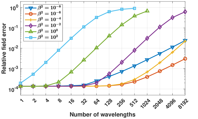
Figure 1: Relative field error of the ultraweak DPG Maxwell solution for the fundamental TE mode in a homogeneous 3D rectangular waveguide. The discretization is uniformly fifth-order with a fixed number of elements per wavelength. Choosing a small scaling constant $\beta$ in the DPG test norm improves the stability of the method significantly, but choosing $\beta$ too small results in round-off errors that adversely affect the solution.

We recall the scaled adjoint graph norm from Section 2:

$$\|v\|^{2}_{H_{A^{*}}(\Omega_{h})}=\|A_{h}^{*}v\|^{2}+\beta^{2}\|v\|^{2}.$$

The analysis of Lemma 2.1 and Theorem 4.5 suggests scaling $\beta$ with $L^{-1}$ to maintain stability of the method as the waveguide length $L$ increases. Figure 1 shows the relative $L^{2}$-error of the electric field $\bm{E}$ for various choices of $\beta$ and increasing waveguide length. The numerical results confirm that the choice of $\beta$ indeed significantly affects the stability of the discretization. In practice, of course, scaling $\beta$ is limited due to rounding errors as $\beta$ becomes very small (or very large). In our experiments, the best results were obtained for $\beta^{2}=10^{-6}$. In other words, by choosing $\beta$ sufficiently small, ultraweak DPG can compensate (to a certain extent) the loss of stability due to the $L^{-1}$ dependence of the boundedness-below constant.

Conclusions. Non-homogeneous waveguide.

The convergence analysis for the DPG method for the modified Maxwell model resulting from a full envelope ansatz led us to the stability analysis for EM waveguides. We started with a simpler, acoustic waveguide, and then proceeded to the homogeneous Maxwell model. For both models, we have obtained the same result: the stability constant depends linearly on the length of the waveguide, i.e.,

$$\|\bm{E}\|+\|\bm{H}\|\leq CL\left(\|\bm{\nabla}\times\bm{E}-i\omega\bm{H}\|+\|\bm{\nabla}\times\bm{H}+i\omega\bm{E}\|\right)\,,\qquad C>0\,.$$

For the non-homogeneous optical waveguide, $\mu=1$, $\epsilon=1+\delta\epsilon$, the triangle inequality implies:

$$\|\bm{E}\|+\|\bm{H}\| \leq CL\left(\|\bm{\nabla}\times\bm{E}-i\omega\bm{H}\|+\|\bm{\nabla}\times\bm{H}+i\omega(1+\delta\epsilon-\delta\epsilon)\bm{E}\|\right)$$

$$\leq CL\left(\|\bm{\nabla}\times\bm{E}-i\omega\bm{H}\|+\|\bm{\nabla}\times\bm{H}+i\omega(1+\delta\epsilon)\bm{E}\|+\omega\|\delta\epsilon\|_{L^{\infty}}\|\bm{E}\|\right)\,.$$

Consequently,

$$(1-CL\omega\|\delta\epsilon\|_{L^{\infty}}\omega)(\|\bm{E}\|+\|\bm{H}\|)\leq CL\left(\|\bm{\nabla}\times\bm{E}-i\omega\bm{H}\|+\|\bm{\nabla}\times\bm{H}+i\omega(1+\delta\epsilon)\bm{E}\|\right)\,,$$

which proves that, for a sufficiently small perturbation $\delta\epsilon$, the operator remains bounded below. However, the information about the linear dependence of the stability constant upon $L$ is lost. In fact, the larger $L$, the smaller $\delta\epsilon$ is allowed. In the second part of this work [7], we generalize our results to the case of non-homogeneous waveguides using perturbation theory.

Appendix A Proof of Lemma 3.1

For the convenience of the reader and to clarify some arguments from [32] we provide some details of the proof of Lemma 3.1. To simply the notation, we write in the present section

$$a^{1D}_{\kappa}(u,v) =(u^{\prime},v^{\prime})_{L^{2}(0,1)}+\kappa^{2}(u,v)_{L^{2}(0,1)}+\kappa u(1)\overline{v}(1),$$

$$\|u\|^{2}_{1,|\kappa|} :=\|u^{\prime}\|^{2}_{L^{2}(0,1)}+|\kappa|^{2}\|u\|^{2}_{L^{2}(0,1)}$$

Lemma A.1 ([32, Lemma 4.1])

For any $\kappa\in\mathbb{C}_{\geq 0}\setminus\{0\}$, the sesquilinear form $a^{1D}_{\kappa}$ satisfies

$$\inf_{u\in V\setminus\{0\}}\sup_{v\in V\setminus\{0\}}\frac{\operatorname*{Re}a^{1D}_{\kappa}(u,v)}{\|u\|_{1,|\kappa|}\|v\|_{1,|\kappa|}}\geq\frac{\operatorname*{Re}\kappa}{|\kappa|}.$$

Proof:     Given $u\in V$ take $v:=\frac{\kappa}{|\kappa|}u\in V$ and compute

$$\operatorname*{Re}a^{1D}_{\kappa}(u,v) =\operatorname*{Re}\left(\frac{\overline{\kappa}}{|\kappa|}\|u^{\prime}\|^{2}_{L^{2}(0,1)}+\kappa|\kappa|\|u\|^{2}_{L^{2}(0,1)}+|\kappa||u(1)|^{2}\right)\geq\frac{\operatorname*{Re}\kappa}{|\kappa|}\|u\|^{2}_{1,|\kappa|}=\frac{\operatorname*{Re}\kappa}{|\kappa|}\|u\|_{1,|\kappa|}\|v\|_{1,|\kappa|}.$$

 

The following is a corrected proof (restricted to the presently considered 1D situation) of [32, Lemma 4.2]. The statement of [32, Lemma 4.2] is, however, correct (cf. Cor. A.3 below).

Lemma A.2 ([32, Lemma 4.2])

Let $V=H^{1}(0,1)$ or $V=H^{1}_{(0}(0,1)$. There is $C>0$ such that for all $\kappa\in\mathbb{C}_{\geq 0}$ with $|\kappa|\geq 1$ and all $f\in L^{2}(0,1)$, $g\in\mathbb{C}$ the solution $u\in V$ of

$$a^{1D}_{\kappa}(u,v)=(f,v)_{L^{2}(0,1)}+g\overline{v}(1)\quad\forall v\in V$$

satisfies the stability bound

$$\|u\|_{1,|\kappa|}\leq C\left[\|f\|_{L^{2}(0,1)}+|g|\right].$$

Proof:     This is taken from [32, Lemma 4.2], where the multidimensional case is covered. We repeat the arguments, which are based on the multiplier technique worked out in detail in [31, Lemma 4.2], [12, Cor. 2.11], [30, Prop. 8.1.3].

Case a: For a parameter $\beta>0$, consider the case $|\operatorname*{Im}\kappa|\leq\beta\operatorname*{Re}\kappa$. In view of $|\kappa|\geq 1$, this implies

$$\operatorname*{Re}\kappa\geq\frac{1}{\sqrt{1+\beta^{2}}}|\kappa|\geq\frac{1}{\sqrt{1+\beta^{2}}}.$$

By the inf-sup condition satisfied by $a^{1D}_{\kappa}$ in view of Lemma A.1 so that the solution $u$ satisfies by the variational formulation

$$\|u\|^{2}_{1,|\kappa|} \leq C_{\beta}\left[\|f\|_{L^{2}(0,1)}\|u\|_{L^{2}(0,1)}+|g||u(1)|\right]\leq C_{\beta}\left[\frac{1}{|\kappa|}\|f\|_{L^{2}(0,1)}+\frac{1}{\sqrt{|\kappa|}}|g|\right]\|u\|_{1,|\kappa|}.$$

In view of $\operatorname*{Re}\kappa\geq 1/\sqrt{(1+\beta^{2})}$ and $|\kappa|\geq\operatorname*{Re}\kappa$, this is a stronger result than needed (cf. Cor. A.3 ahead).

Case b: We consider the case $|\operatorname*{Im}\kappa|\geq\beta\operatorname*{Re}\kappa$ so that

$$|\operatorname*{Im}\kappa|\leq|\kappa|\leq\left(1+\beta^{-1}\right)|\operatorname*{Im}\kappa|.$$

Taking as the test function $v=u$ gives by taking the real part

$$\|u^{\prime}\|^{2}_{L^{2}(0,1)}+\operatorname*{Re}\kappa^{2}\|u\|^{2}_{L^{2}(0,1)}+\operatorname*{Re}\kappa|u(1)|^{2} \lesssim\|f\|_{L^{2}(0,1)}\|u\|_{L^{2}(0,1)}+|g||u(1)|.$$ (A.1)

Taking as the test function $v=(\operatorname*{Im}\kappa)u$ gives by taking the imaginary part

$$2\underbrace{|\operatorname*{Im}\kappa|\operatorname*{Re}\kappa}_{\geq 0}\|u\|^{2}_{L^{2}(0,1)}+|\operatorname*{Im}\kappa||u(1)|^{2} \lesssim\|f\|_{L^{2}(0,1)}\|u\|_{L^{2}(0,1)}+|g||u(1)|.$$ (A.2)

The multiplier technique amounts to taking as a test function $v=xu^{\prime}$. Using the relations

$$\operatorname*{Re}u^{\prime}(x\overline{u}^{\prime})^{\prime} =\frac{1}{2}x\left(|u^{\prime}|^{2}\right)^{\prime}+|u^{\prime}|^{2}, \operatorname*{Re}ux\overline{u}^{\prime} =\frac{1}{2}x\left(|u|^{2}\right)^{\prime}, \operatorname*{Im}ux\overline{u} =0$$

we get for the test function $v=xu^{\prime}$

$$\operatorname*{Re}a^{1D}_{\kappa}(u,xu^{\prime}) =\operatorname*{Re}(u^{\prime},(xu^{\prime})^{\prime})_{L^{2}(0,1)}+\operatorname*{Re}\kappa^{2}(u,xu)_{L^{2}(0,1)}+\operatorname*{Re}\kappa u(1)\overline{u}^{\prime}(1)$$

$$=\|u^{\prime}\|^{2}_{L^{2}(0,1)}-\frac{1}{2}\|u^{\prime}\|^{2}_{L^{2}(0,1)}+\frac{1}{2}|u^{\prime}(1)|^{2}-\operatorname*{Re}\kappa^{2}\frac{1}{2}\|u\|^{2}_{L^{2}(0,1)}+\operatorname*{Re}\kappa^{2}\frac{1}{2}|u(1)|^{2}+\operatorname*{Re}\kappa u(1)\overline{u}^{\prime}(1),$$

so that we arrive from the weak formulation of $u$ at

$$\|u^{\prime}\|^{2}_{L^{2}(0,1)}-\operatorname*{Re}\kappa^{2}\|u\|^{2}_{L^{2}(0,1)}+|u^{\prime}(1)|^{2} \leq 2\left(\|f\|_{L^{2}(0,1)}\|xu^{\prime}\|_{L^{2}(0,1)}+|g||u^{\prime}(1)|+|\operatorname*{Re}\kappa||u(1)||u^{\prime}(1)|\right)$$

We note that for sufficiently large $\beta$ we have $\operatorname*{Re}\kappa^{2}=(\operatorname*{Re}\kappa)^{2}-(\operatorname*{Im}\kappa)^{2}\sim-|\kappa|^{2}$. Hence, appropriate Young inequalities yield

$$\|u^{\prime}\|^{2}_{L^{2}(0,1)}|\kappa|^{2}\|u\|^{2}_{L^{2}(0,1)}+|u^{\prime}(1)|^{2} \lesssim\|f\|^{2}_{L^{2}(0,1)}+|g|^{2}+(\operatorname*{Re}\kappa)^{2}|u(1)|^{2}.$$

Young’s inequality applied to (A.2) allows us to remove the term $(\operatorname*{Re}\kappa)^{2}|u(1)|^{2}$.       

We are now in position to prove Lemma 3.1:

Proof of Lemma 3.1: We follow [32, Thm. 4.3]. For $\operatorname*{Re}\kappa\geq 1/\sqrt{2}$ we have by Lemma A.1

$$\inf_{u\in V}\sup_{v\in V}\frac{\operatorname*{Re}a_{\kappa}(u,v)}{\|u\|_{1,|\kappa|}\|v\|_{1,|\kappa|}}\geq\frac{\operatorname*{Re}\kappa}{|\kappa|}=\frac{\operatorname*{Re}\kappa}{\sqrt{(\operatorname*{Re}\kappa)^{2}+(\operatorname*{Im}\kappa)^{2}}}\geq\frac{\operatorname*{Re}\kappa}{\operatorname*{Re}\kappa+|\operatorname*{Im}\kappa|}\geq\frac{1}{1+c\frac{|\operatorname*{Im}\kappa|}{1+\operatorname*{Re}\kappa}},\qquad c=1+\sqrt{2}.$$

Let $\operatorname*{Re}\kappa\leq 1/\sqrt{2}$. Given $u\in V$, we seek $v$ in the form $v=u+z$ with $z$ solving

$$a_{\overline{\kappa}}(z,w)=\alpha^{2}(u,w)_{L^{2}(0,1)}\quad\forall w\in V,\qquad\alpha^{2}:=|\kappa|^{2}-{\kappa}^{2}=-2i(\operatorname*{Im}\kappa)\kappa.$$

By Lemma A.2, we get

$$\|z\|_{1,|\kappa|}\leq C|\alpha|^{2}\|u\|_{L^{2}(0,1)}\leq C|\operatorname*{Im}\kappa||\kappa|\|u\|_{L^{2}(0,1)}$$

and note

$$\operatorname*{Re}a_{\kappa}(u,u+z) =\|u^{\prime}\|^{2}_{L^{2}(0,1)}+\operatorname*{Re}\kappa^{2}\|u\|^{2}_{L^{2}(0,1)}+\operatorname*{Re}\kappa|u(1)|^{2}+\operatorname*{Re}a_{\kappa}(u,z)$$

$$=\|u^{\prime}\|^{2}_{L^{2}(0,1)}+\operatorname*{Re}\kappa^{2}\|u\|^{2}_{L^{2}(0,1)}+\operatorname*{Re}\kappa|u(1)|^{2}+\operatorname*{Re}a_{\overline{\kappa}}(z,u)$$

$$=\|u^{\prime}\|^{2}_{L^{2}(0,1)}+\operatorname*{Re}\kappa^{2}\|u\|^{2}_{L^{2}(0,1)}+\operatorname*{Re}\kappa|u(1)|^{2}+\operatorname*{Re}\alpha^{2}\|u\|^{2}_{L^{2}(0,1)}$$

$$=\|u\|^{2}_{1,|\kappa|}+\underbrace{\operatorname*{Re}\kappa}_{\geq 0}|u(1)|^{2}\geq\|u\|^{2}_{1,|\kappa|}$$

as well as

$$\|u+z\|_{1,|\kappa|}\leq\|u\|_{1,|\kappa|}+\|z\|_{1,|\kappa|}\leq(1+C|\operatorname*{Im}\kappa|)|\kappa|\|u\|_{L^{2}(0,1)}\leq(1+C|\operatorname*{Im}\kappa|)\|u\|_{1,|\kappa|}$$ (A.3)

so that we arrive at

$$\operatorname*{Re}a^{1D}_{\kappa}(u,v)=\operatorname*{Re}a^{1D}_{\kappa}(u,u+z)=\|u\|^{2}_{1,|\kappa|}\geq\frac{\|u\|_{1,|\kappa|}\|u+z\|_{1,|\kappa|}}{1+C|\operatorname*{Im}\kappa|}\geq\frac{\|u\|_{1,|\kappa|}\|u+z\|_{1,|\kappa|}}{1+C\frac{|\operatorname*{Im}\kappa|}{1+\operatorname*{Re}\kappa}}.$$

$\Box$

From the inf-sup condition, we can actually infer the statement of [32, Lemma 4.2]:

Corollary A.3

Let $V=H^{1}(0,1)$ or $V=H^{1}_{(0}(0,1)$. There is $C>0$ such that for all $\kappa\in\mathbb{C}_{\geq 0}$ with $|\kappa|\geq 1$ and all $f\in L^{2}(0,1)$, $g\in\mathbb{C}$ the solution $u\in V$ of

$$a^{1D}_{\kappa}(u,v)=(f,v)_{L^{2}(0,1)}+g\overline{v}(1)\quad\forall v\in V$$

satisfies the stability bound

$$\|u\|_{1,|\kappa|}\leq C\left[\frac{1}{1+\operatorname*{Re}\kappa}\|f\|_{L^{2}(0,1)}+\frac{1}{\sqrt{1+\operatorname*{Re}\kappa}}|g|\right].$$

Proof:     With the inf-sup constant $\gamma_{\kappa}$ of Lemma 3.1 in hand, we get

$$\|u\|_{1,|\kappa|}\leq\frac{C}{\gamma_{\kappa}}\left[\frac{1}{|\kappa|}\|f\|_{L^{2}(0,1)}+\frac{1}{\sqrt{|\kappa|}}|g|\right].$$

We have

$$\frac{1}{\gamma_{\kappa}}\frac{1}{|\kappa|}\sim\frac{1}{1+C\frac{|\operatorname*{Im}\kappa|}{1+\operatorname*{Re}\kappa}}\frac{1}{|\operatorname*{Im}\kappa|+\operatorname*{Re}\kappa}$$

and now distinguish between the cases $|\operatorname*{Im}\kappa|\leq 1/2$ (which implies $\operatorname*{Re}\kappa\geq\sqrt{3/4}$ by the requirement $|\kappa|\geq 1$) and the case $|\operatorname*{Im}\kappa|\geq 1/2$. In the first case, we have $|\operatorname*{Im}\kappa|/\operatorname*{Re}\kappa\leq c$ for some $c>0$ and can simply

$$\frac{1}{1+C\frac{|\operatorname*{Im}\kappa|}{1+\operatorname*{Re}\kappa}}\frac{1}{|\operatorname*{Im}\kappa|+\operatorname*{Re}\kappa}\sim\frac{1}{\operatorname*{Re}\kappa}\frac{1}{1+\frac{|\operatorname*{Im}\kappa|}{\operatorname*{Re}\kappa}}\frac{1}{1+\frac{|\operatorname*{Im}\kappa|}{\operatorname*{Re}\kappa}}\sim\frac{1}{\operatorname*{Re}\kappa}.$$

In the second case, we have $|\operatorname*{Im}\kappa|/\operatorname*{Re}\kappa\geq c>0$ and can estimate

$$\frac{1}{1+C\frac{|\operatorname*{Im}\kappa|}{1+\operatorname*{Re}\kappa}}\frac{1}{|\operatorname*{Im}\kappa|+\operatorname*{Re}\kappa}=\frac{1}{\operatorname*{Re}\kappa}\frac{1}{1+C\frac{|\operatorname*{Im}\kappa|}{1+\operatorname*{Re}\kappa}}\frac{1}{\frac{|\operatorname*{Im}\kappa|}{\operatorname*{Re}\kappa}}\leq\frac{1}{\operatorname*{Re}\kappa}\frac{1}{c}.$$

We conclude that the prefactor of the term $\|f\|_{L^{2}(0,1)}$ has the desired form. The estimate for the prefactor of $|g|$ is analogous.       

Appendix B Reduction of the first-order system to second equations for Maxwell’s equations

B.1 The system for $\bm{\alpha_{i}}$, $\bm{\delta_{i}}$, $\bm{\zeta_{i}}$

We consider (4.16a), (4.16c), (4.16d), viz., (skipping the subscript $i$)

$$\alpha^{\prime}-i{\omega}\delta =f_{1},$$ (B.1)

$$\alpha-i{\omega}\mu^{-1}\zeta =f_{3},$$ (B.2)

$$-\delta^{\prime}+\zeta+i{\omega}\alpha =g_{1}.$$ (B.3)

Multiplying (B.2) with $\mu$ and (B.3) with $i{\omega}$ and addiing the equations, we eliminate $\zeta$ and obtain

$$\alpha^{\prime}-i{\omega}\delta =f_{1},$$ (B.4)

$$-i{\omega}\delta^{\prime}+\underbrace{(\mu-{\omega}^{2})}_{=:\widetilde{\mu}^{2}}\alpha =i{\omega}g_{1}+\mu f_{3}.$$ (B.5)

On $(L,\infty)$, this system corresponds to the right-hand sides $f_{1}=f_{3}=g_{1}=0$. By eliminating $\delta$ we get

$$\alpha^{\prime\prime}-\widetilde{\mu}^{2}\alpha=0$$

with fundamental system $e^{\pm\widetilde{\mu}z}$. The requirement of outgoing waves implies that we seek solutions of the homogeneous system as multiples of $e^{-\widetilde{\mu}z}$, which provides us with the boundary condition at $z=L$

$$\alpha^{\prime}(L)+\widetilde{\mu}\alpha(L)=0.$$ (B.6)

In view of (B.1) on $(L,\infty)$ with $f_{1}=0$ we obtain

$$0\stackrel{{\scriptstyle(\ref{eq:maxwell-1-hinten})}}{{=}}\alpha^{\prime}(L)-i{\omega}\delta(L)\stackrel{{\scriptstyle(\ref{eq:impedance-bc-alpha-hinten})}}{{=}}-\widetilde{\mu}\alpha(L)-i{\omega}\delta(L).$$ (B.7)

We also have the boundary condition

$$\alpha(0)=0.$$ (B.8)

We now turn to the weak formulation. For $v$ with $v(0)=0$ we get by multiplying (B.4) by $v^{\prime}$ and integrating over $(0,L)$ and by multiplying (B.5) by $v$ and integrating over $(0,L)$

$$(\alpha^{\prime},v^{\prime})_{L^{2}(0,L)}-i{\omega}(\delta,v^{\prime})_{L^{2}(0,L)} =(f_{1},v^{\prime})_{L^{2}(0,L)},$$ (B.9)

$$-i{\omega}(\delta^{\prime},v)_{L^{2}(0,L)}+\widetilde{\mu}^{2}(\alpha,v)_{L^{2}(0,L)} =i{\omega}(g_{1},v)_{L^{2}(0,L)}+\mu(f_{3},v)_{L^{2}(0,L)}.$$ (B.10)

Integrating the term $(\delta^{\prime},v)_{L^{2}(0,L)}$ by parts and using $v(0)=0$ as well as $i{\omega}\delta(L)=-\widetilde{\mu}\alpha(L)$ by (B.7) gives

$$(\alpha^{\prime},v^{\prime})_{L^{2}(0,L)}-i{\omega}(\delta,v^{\prime})_{L^{2}(0,L)} =(f_{1},v^{\prime})_{L^{2}(0,L)},$$ (B.11)

$$i{\omega}(\delta,v^{\prime})_{L^{2}(0,L)}+\widetilde{\mu}\alpha(L)\overline{v}(L)+\widetilde{\mu}^{2}(\alpha,v)_{L^{2}(0,L)} =i{\omega}(g_{1},v)_{L^{2}(0,L)}+\mu(f_{3},v)_{L^{2}(0,L)}.$$ (B.12)

Adding these two equations yields

$$(\alpha^{\prime},v^{\prime})_{L^{2}(0,L)}+\widetilde{\mu}^{2}(\alpha,v)_{L^{2}(0,L)}+\widetilde{\mu}\alpha(L)\overline{v}(L) =(f_{1},v^{\prime})_{L^{2}(0,L)}+i{\omega}(g_{1},v)_{L^{2}(0,L)}+\mu(f_{3},v)_{L^{2}(0,L)}.$$ (B.13)

B.2 The system for $\bm{\beta_{j}}$, $\bm{\gamma_{j}}$, $\bm{\eta_{j}}$

We consider (4.16b), (4.16e), (4.16f), viz., (skipping the subscript $j$)

$$-\beta^{\prime}+\gamma-i{\omega}\eta =f_{2},$$ (B.14)

$$\eta^{\prime}+i{\omega}\beta =g_{2},$$ (B.15)

$$\eta+i{\omega}\lambda^{-1}\gamma =g_{3}.$$ (B.16)

Multiplying (B.14) with $i{\omega}$, (B.16) with $\lambda$ and subtracting the equations, we get

$$-i{\omega}\beta^{\prime}-\widetilde{\lambda}^{2}\eta =i{\omega}f_{2}-\lambda g_{3},$$ (B.17)

$$\widetilde{\lambda}^{2}\eta^{\prime}+i{\omega}\widetilde{\lambda}^{2}\beta =\widetilde{\lambda}^{2}g_{2},$$ (B.18)

where we also multiplied (B.15) by $\widetilde{\lambda}^{2}:={\lambda-\omega^{2}}$. On $(L,\infty)$, this system corresponds to the right-hand sides $f_{2}=g_{2}=g_{3}=0$. By eliminating $\eta$ we get

$$-\beta^{\prime\prime}+\widetilde{\lambda}^{2}\beta=0$$

with fundamental system $e^{\pm\widetilde{\lambda}z}$. The requirement of outgoing waves implies that we seek solutions of the homogeneous system as multiples of $e^{-\widetilde{\lambda}z}$, which provides us with the boundary condition at $z=L$

$$\beta^{\prime}(L)+\widetilde{\lambda}\beta(L)=0.$$ (B.19)

In view of (B.17) on $(L,\infty)$ with $f_{2}=g_{3}=0$ we obtain

$$0\stackrel{{\scriptstyle(\ref{eq:maxwell-2-hinten-1})}}{{=}}-i{\omega}\beta^{\prime}(L)-\widetilde{\lambda}^{2}\eta(L)\stackrel{{\scriptstyle(\ref{eq:impedance-bc-beta-hinten})}}{{=}}i{\omega}\widetilde{\lambda}\beta(L)-\widetilde{\lambda}^{2}\eta(L).$$ (B.20)

We also have the boundary condition

$$\beta(0)=0.$$ (B.21)

We now turn to the weak formulation. For $v$ with $v(0)=0$ we get by multiplying (B.17) by $v^{\prime}$ and integrating over $(0,L)$ and by multiplying (B.18) by $v$ and integrating over $(0,L)$

$$-i{\omega}(\beta^{\prime},v^{\prime})_{L^{2}(0,L)}-\widetilde{\lambda}^{2}(\eta,v^{\prime})_{L^{2}(0,L)} =i{\omega}(f_{2},v^{\prime})_{L^{2}(0,L)}-\lambda(g_{3},v^{\prime}),$$ (B.22)

$$\widetilde{\lambda}^{2}(\eta^{\prime},v)_{L^{2}(0,L)}+i{\omega}\widetilde{\lambda}^{2}(\beta,v)_{L^{2}(0,L)} =\widetilde{\lambda}^{2}(g_{2},v)_{L^{2}(0,L)}.$$ (B.23)

Integrating the term $(\eta^{\prime},v)_{L^{2}(0,L)}$ by parts and using $v(0)=0$ as well as $\widetilde{\lambda}^{2}\eta(L)=i{\omega}\widetilde{\lambda}\beta(L)$ by (B.20) gives

$$-i{\omega}(\beta^{\prime},v^{\prime})_{L^{2}(0,L)}-\widetilde{\lambda}^{2}(\eta,v^{\prime})_{L^{2}(0,L)} =i{\omega}(f_{2},v^{\prime})_{L^{2}(0,L)}-\lambda(g_{3},v^{\prime}),$$ (B.24)

$$-\widetilde{\lambda}^{2}(\eta,v^{\prime})_{L^{2}(0,L)}+i{\omega}\widetilde{\lambda}\beta(L)\overline{v}(L)+i{\omega}\widetilde{\lambda}^{2}(\beta,v)_{L^{2}(0,L)} =\widetilde{\lambda}^{2}(g_{2},v)_{L^{2}(0,L)}.$$ (B.25)

Subtracting these two equations yields

$$-i{\omega}(\beta^{\prime},v^{\prime})_{L^{2}(0,L)}-i{\omega}\widetilde{\lambda}^{2}(\beta,v)_{L^{2}(0,L)}-i{\omega}\widetilde{\lambda}\beta(L)\overline{v}(L) =i{\omega}(f_{2},v^{\prime})_{L^{2}(0,L)}-\lambda(g_{3},v^{\prime})-\widetilde{\lambda}^{2}(g_{2},v)_{L^{2}(0,L)},$$ (B.26)

i.e.,

$$(\beta^{\prime},v^{\prime})_{L^{2}(0,L)}+\widetilde{\lambda}^{2}(\beta,v)_{L^{2}(0,L)}+\widetilde{\lambda}\beta(L)\overline{v}(L) =-(f_{2},v^{\prime})_{L^{2}(0,L)}+\frac{\lambda}{i{\omega}}(g_{3},v^{\prime})+\widetilde{\lambda}^{2}\frac{1}{i{\omega}}(g_{2},v)_{L^{2}(0,L)}.$$ (B.27)

Appendix C $\operatorname{DtN}$ for the Maxwell problem in $\Omega$

Recall $\Gamma_{-}:=\partial\Omega\setminus\overline{\Gamma_{\text{out}}}$ and $\bm{H}_{0,\Gamma_{-}}(\operatorname{curl},{\Omega}):=\{\bm{E}\in\bm{H}(\operatorname{curl},{\Omega})\,|\,\gamma_{t}\bm{E}=0\mbox{ on $\Gamma_{-}$}\}$. We also recall the tangential component operator $\pi_{t}$.

C.1 Derivation of the ODE system (4.16)

We start with

Lemma C.1

For $\psi\in H^{1}(D)$ and $w\in L^{2}(0,L)$ there holds in the sense of distributions

$$\operatorname{curl}\left(w\left(\begin{array}[]{c}\bm{\nabla}\times\psi\\ 0\end{array}\right)\right) =\left(\begin{array}[]{c}w^{\prime}\bm{\nabla}\psi\\ -w\Delta\psi\end{array}\right), \operatorname{curl}\left(w\left(\begin{array}[]{c}\bm{\nabla}\psi\\ 0\end{array}\right)\right) =-\left(\begin{array}[]{c}w^{\prime}\bm{\nabla}\times\psi\\ 0\end{array}\right), \operatorname{curl}(\bm{e}_{z}\psi w) =\left(\begin{array}[]{c}w\bm{\nabla}\times\psi\\ 0\end{array}\right).$$

Here, the expressions $\Delta\psi$ and $w^{\prime}$ are understood in the sense of distributions (in $D$ and $(0,L)$, respectively).

Proof:     This is a calculation.       

Next, we give more details about the derivation of the equations (4.16):

Lemma C.2

Let $\bm{f}$, $\bm{g}\in L^{2}({\Omega})$, and let the functions $\bm{E}\in\bm{H}_{\Gamma_{-}}(\operatorname{curl},{\Omega})$, $\bm{H}\in\bm{H}(\operatorname{curl},{\Omega})$ satisfy (2.4a)–(2.4d). Let the coefficients $\alpha_{i}$, $\beta_{i}$, $\gamma_{i}$, $\delta_{i}$, $\eta_{i}$, and $\zeta_{i}$ of the functions $\bm{E}$, $\bm{H}$ be given by (4.15). Then these coefficients satisfy the ODE system (4.16) in the sense of distributions. Additionally, the functions $\gamma_{i}$, $\zeta_{i}\in L^{2}(0,L)$ and $\alpha_{i}$, $\beta_{i}$, $\delta_{i}$, $\eta_{i}\in H^{1}(0,L)$ so that the ODE system (4.16) holds in a weak sense and pointwise almost everywhere.

Proof:     Since the functions $\bm{E}$, $\bm{H}\in L^{2}({\Omega})$, we have that $\alpha_{i}$, $\beta_{i}$, $\gamma_{i}$, $\delta_{i}$, $\eta_{i}$, $\zeta_{i}\in L^{2}(0,L)$. To derive the formulas (4.16), we note that $(\bm{E},\bm{H})$ satisfies, for $\bm{F}$, $\bm{G}\in L^{2}({\Omega})$

$$(\bm{\nabla}\times\bm{E},\bm{F})_{L^{2}({\Omega})}-i{\omega}(\bm{H},\bm{F})_{L^{2}({\Omega})} =(\bm{f},\bm{F})_{L^{2}({\Omega})},$$ (C.1)

$$(\bm{\nabla}\times\bm{H},\bm{G})_{L^{2}({\Omega})}+i{\omega}(\bm{H},\bm{G})_{L^{2}({\Omega})} =(\bm{f},\bm{G})_{L^{2}({\Omega})}.$$ (C.2)

The equations (4.16) are obtained by suitably choosing the test functions $\bm{F}$, $\bm{G}$. We illustrate the procedure for (4.16a) by taking $\bm{F}=w(z)\left(\begin{array}[]{c}\bm{\nabla}\psi_{i}\\ 0\end{array}\right)$ with $w\in C^{\infty}_{0}(0,L)$. We note that $\bm{F}\in\bm{H}(\operatorname{curl},{\Omega})$ with

$$\bm{\nabla}\times\bm{F}=-\left(\begin{array}[]{c}w^{\prime}\bm{\nabla}\psi_{i}\\ 0\end{array}\right)\in L^{2}({\Omega})$$

by Lemma C.1. In view of $w\in C^{\infty}_{0}(0,L)$ and the boundary conditions satisfied by $\bm{E}$ (cf. (2.4c)) we observe $(\gamma_{t}\bm{E},\pi_{t}\bm{F})=0$. Hence an integration by parts and the fact that the expansion of $\bm{E}$ converges in $L^{2}({\Omega})$ as well as the orthogonalities satisfied by the functions $\psi_{i}$, $\phi_{i}$ gives

$$(\bm{\nabla}\times\bm{E},\bm{F})_{L^{2}({\Omega})} =(\bm{E},\bm{\nabla}\times\bm{F})_{L^{2}({\Omega})}=-\int_{z=0}^{L}\alpha_{i}(z)w^{\prime}(z).$$ (C.3)

Hence, we get from (C.1) and (C.3) with the orthogonalities satisfied by the functions $\psi_{i}$, $\phi_{i}$

$$\int_{z=0}^{L}-\alpha_{i}(z)w^{\prime}(z)+\delta_{i}(z)w(z)\,dz =\int_{z=0}^{L}w(z)(\bm{f},\left(\begin{array}[]{c}\nabla\psi_{i}\\ 0\end{array}\right))_{L^{2}(D)}\,dz=\int_{z=0}^{L}w(z)f_{i,1}w(z)\,dz,$$

which is the (distributional) form of (4.16a). The remaining 5 equations in (4.16) are obtained similarly with suitable test functions; we note that in the choice of $\bm{G}$, one takes functions such that $\bm{G}\in\bm{H}_{0}(\operatorname{curl},{\Omega})$ so that an integration by parts as in (C.3) is again possible.

Since the right-hand sides $f_{i,1},\ldots,g_{i,3}$ are in $L^{2}(0,L)$, the system (4.16) shows that $\alpha_{i}$, $\beta_{i}$, $\delta_{i}\in H^{1}(0,L)$.       

C.2 Mapping properties of the $\operatorname{DtN}^{\operatorname{mw}}$-operator

We note that by [11, Prop. 3.6] the space $\{\bm{u}\in(C^{\infty}(\overline{{\Omega}}))^{3}\,|\,\gamma_{t}\bm{u}=0\mbox{ in a neighborhood of $\overline{\Gamma_{-}}$}\}$ is dense in $\bm{H}_{0,\Gamma_{-}}(\operatorname{curl},{\Omega})$.

In order to define the $\operatorname{DtN}$-operator, we introduce with the eigenpairs $(\psi_{j},\mu_{j})_{j}$ and $(\phi_{i},\lambda_{i})_{i}$ on the space of sufficiently smooth functions the linear functionals (we identify in the canonical way $\Gamma_{\text{out}}\subset\mathbb{R}^{3}$ with $D\subset\mathbb{R}^{2}$, on which the eigenfunctions $\phi_{i}$, $\psi_{j}$ are defined):

$$\hat{\alpha}_{i}(\bm{E}) :=(\pi_{t}\bm{E},\bm{\nabla}\times\psi_{i})_{L^{2}(\Gamma_{\text{out}})},$$ (C.4)

$$\hat{\beta}_{j}(\bm{E}) :=(\pi_{t}\bm{E},\bm{\nabla}\phi_{j})_{L^{2}(\Gamma_{\text{out}})}.$$ (C.5)

We next show that these linear functionals can be uniquely extended to continuous linear functionals on $\bm{H}_{0,\Gamma_{-}}(\operatorname{curl},{\Omega})$:

Theorem C.3

There is $C>0$ depending only on $\Omega$ and $\Gamma_{-}$ such that for all $\bm{E}\in\bm{H}_{0,\Gamma_{-}}(\operatorname{curl},{\Omega})$

$$\sum_{i\geq 2}|\hat{\alpha}_{i}(\bm{E})|^{2}\mu_{i}^{1/2} \leq C\|\bm{E}\|^{2}_{\bm{H}(\operatorname{curl},{\Omega})},$$

$$\sum_{j\geq 1}|\hat{\beta}_{j}(\bm{E})|^{2}\lambda_{j}^{-1/2} \leq C\|\bm{E}\|^{2}_{\bm{H}(\operatorname{curl},{\Omega})}.$$

Proof:     Step 1: By the arguments given in [3, pp. 28/29], we can decompose $\bm{E}=\bm{\psi}+\nabla p$ with $\bm{\psi}\in\bm{H}^{1}({\Omega})\cap\bm{H}_{0,\Gamma_{-}}(\operatorname{curl},{\Omega})$ and $p\in H^{1}_{\Gamma_{-}}(\Omega)$ together with the stability estimate

$$\|\bm{\psi}\|_{\bm{H}^{1}({\Omega})}+\|p\|_{H^{1}({\Omega})} \leq C\|\bm{E}\|_{\bm{H}(\operatorname{curl},{\Omega})}.$$ (C.6)

Step 2: By the density result [11, Prop. 3.6], we may assume in Steps 3–6 that $\bm{\psi}$ is smooth and vanishes in a neighborhood of $\Gamma_{-}$ as we only need to control $\|\bm{\psi}\|_{\bm{H}(\operatorname{curl},{\Omega})}$. In Step 7, we may assume that $\bm{\psi}$ is smooth and that we control $\|\bm{\psi}\|_{\bm{H}^{1}({\Omega})}$. In Step 7, we may also assume $p|_{\Gamma_{\text{out}}}\in C^{\infty}_{0}(\Gamma_{\text{out}})$ by the the standard density of $C^{\infty}_{0}(\Gamma_{\text{out}})$ in $\widetilde{H}^{1}(\Gamma_{\text{out}})$.

Step 3: With the notation $\bm{H}^{1/2}_{\parallel}(\Gamma)$ of [3, p. 14] and its dual $\bm{H}^{-1/2}_{\parallel}(\Gamma):=\left(\bm{H}^{1/2}_{\parallel}(\Gamma)\right)^{\prime}$ we introduce (cf. [3, p. 22]) $\bm{H}^{-1/2}_{\parallel}(\operatorname{div}_{\Gamma},\Gamma):=\{\bm{u}\in\bm{H}^{-1/2}_{\parallel}(\Gamma)\,|\,\operatorname{div}_{\Gamma}\bm{u}\in H^{-1/2}(\Gamma)\}$. By [3, Thm. 3.9], the mapping $\gamma_{t}:\bm{H}(\operatorname{curl},{\Omega})\rightarrow\bm{H}^{-1/2}_{\parallel}(\operatorname{div}_{\Gamma},\Gamma)$ is continuous. Furthermore, one has

$$\operatorname{div}_{\Gamma}\gamma_{t}\bm{u}=\operatorname{curl}_{\Gamma}\pi_{t}\bm{u}\quad\mbox{ in $H^{-1/2}(\Gamma)$},$$ (C.7)

which follows by a straight-forward calculation for smooth $\bm{u}$ and a density argument.

Step 4: Since $\operatorname{div}_{\Gamma}\gamma_{t}\bm{\psi}\in H^{-1/2}(\Gamma)$ (by the continuity of $\gamma_{t}$) and $\gamma_{t}\bm{\psi}=0$ on $\Gamma_{-}$ we get $\operatorname{div}_{\Gamma}\gamma_{t}\bm{\psi}=0$ in $H^{-1/2}(\Gamma_{-})$. By the density of compactly supported functions in $H^{1/2}(\Gamma_{-})$, [28, Thm. 11.1], we infer the stronger result $\operatorname{div}_{\Gamma}\gamma_{t}\bm{\psi}=0$ in $\left(H^{1/2}(\Gamma_{-})\right)^{\prime}$. From [11, Prop. 3.3], we get the bound

$$\|\operatorname{div}_{\Gamma}\gamma_{t}\bm{\psi}\|_{(H^{1/2}(\Gamma_{\text{out}}))^{\prime}}\leq C\|\operatorname{div}_{\Gamma}\gamma_{t}\bm{\psi}\|_{H^{-1/2}(\Gamma)}\leq C\|\bm{\psi}\|_{\bm{H}(\operatorname{curl},{\Omega})}.$$ (C.8)

Step 5: The operators $\bm{\nabla}\times$ is a continuous mapping $H^{1}(\Gamma_{\text{out}})\rightarrow L^{2}(\Gamma_{\text{out}})$ as well as $L^{2}(\Gamma_{\text{out}})\rightarrow H^{-1}(\Gamma_{\text{out}})$ so that, by interpolation,

$$\|\bm{\nabla}\times\psi_{i}\|_{H^{-1/2}(\Gamma_{\text{out}})} \leq C\|\psi_{i}\|_{H^{1/2}(\Gamma_{\text{out}})}\quad\forall i.$$ (C.9)

We next claim

$$\|\bm{\nabla}\phi_{j}\|_{\widetilde{H}^{-1/2}(\Gamma_{\text{out}})} \leq C\|\phi_{j}\|_{\widetilde{H}^{1/2}(\Gamma_{\text{out}})}\quad\forall j.$$

To see this, we note that the operator $\operatorname{div}$ is a continuous operator $\bm{H}^{1}(\Gamma_{\text{out}})\rightarrow L^{2}(\Gamma_{\text{out}})$ and $\bm{L}^{2}(\Gamma_{\text{out}})\rightarrow H^{-1}(\Gamma_{\text{out}})$ so that by interpolation it is a continuous map $\bm{H}^{1/2}(\Gamma_{\text{out}})\rightarrow H^{-1/2}(\Gamma_{\text{out}})$. Hence, using the boundary conditions satisfied by $\phi_{j}$,

$$\|\nabla\phi_{j}\|_{\widetilde{H}^{-1/2}(\Gamma_{\text{out}})} =\sup_{\bm{v}\in\bm{H}^{1}(\Gamma_{\text{out}})}\frac{(\nabla\phi_{j},\bm{v})_{L^{2}(\Gamma_{\text{out}})}}{\|\bm{v}\|_{\bm{H}^{1/2}(\Gamma_{\text{out}})}}=\sup_{\bm{v}\in\bm{H}^{1}(\Gamma_{\text{out}})}\frac{(\phi_{j},\operatorname{div}\bm{v})_{L^{2}(\Gamma_{\text{out}})}}{\|\bm{v}\|_{\bm{H}^{1/2}(\Gamma_{\text{out}})}}$$

$$\leq\sup_{\bm{v}\in\bm{H}^{1}(\Gamma_{\text{out}})}\|\phi_{j}\|_{\widetilde{H}^{1/2}(\Gamma_{\text{out}})}\frac{\|\operatorname{div}\bm{v}\|_{H^{-1/2}(\Gamma_{\text{out}})}}{\|\bm{v}\|_{H^{1/2}(\Gamma_{\text{out}})}}\leq C\|\phi_{j}\|_{\widetilde{H}^{1/2}(\Gamma_{\text{out}})}.$$

Step 6: (estimating $\hat{\alpha}_{i}$) From the smoothness of $\bm{\psi}$ and since it vanishes in a neighborhood of $\partial\Gamma_{-}$, we get

$$\left|\hat{\alpha}_{i}(\bm{\psi})\right| =\left|(\pi_{t}\bm{\psi},\bm{\nabla}\times\psi_{i})_{L^{2}(\Gamma_{\text{out}})}\right|=\left|(\operatorname{curl}_{\Gamma}\pi_{t}\bm{\psi},\psi_{i})_{L^{2}(\Gamma_{\text{out}})}\right|=\left|(\operatorname{div}_{\Gamma}\gamma_{t}\bm{\psi},\psi_{i})_{L^{2}(\Gamma_{\text{out}})}\right|.$$

Hence, the coefficients $\hat{\alpha}_{i}(\bm{\psi})$ are the coefficients obtained by expanding $\operatorname{div}_{\Gamma}\gamma_{t}\bm{\psi}$ in terms of the functions $(\psi_{i})_{i}$. Since $\|\psi_{i}\|_{L^{2}(\Gamma_{\text{out}})}=\lambda_{i}^{-1/2}$ and (C.8), we get

$$\sum_{i}|\hat{\alpha}_{i}(\bm{\psi})|^{2}\lambda_{i}^{1/2} \sim\|\operatorname{div}_{\gamma}\gamma\bm{\psi}\|^{2}_{\widetilde{H}^{-1/2}(\Gamma_{\text{out}})}\stackrel{{\scriptstyle(\ref{eq:thm:alphai-betaj-20})}}{{\lesssim}}\|\bm{\psi}\|^{2}_{\bm{H}(\operatorname{curl},{\Omega})}.$$

Since $p\in\widetilde{H}^{1/2}(\Gamma_{\text{out}})$, we compute with an integration by parts

$$\hat{\alpha}_{i}(\nabla p) =(\nabla p,\bm{\nabla}\times\psi_{i})_{L^{2}(\Gamma_{\text{out}})}=0.$$

Step 7: (estimating $\hat{\beta}_{j}$) Using that $\phi_{j}\in\widetilde{H}^{1/2}(\Gamma_{\text{out}})$, an integration by parts gives

$$\hat{\beta}_{j}(\bm{\psi}) =(\pi_{t}\bm{\psi},\nabla\phi_{j})_{L^{2}(\Gamma_{\text{out}})}=-(\operatorname{div}_{\Gamma}\pi_{t}\bm{\psi},\phi_{j})_{L^{2}(\Gamma_{\text{out}})}.$$

Hence, the coefficients $\hat{\beta}_{j}(\bm{\psi})$ are the coefficients obtained by expanding $\operatorname{div}_{\Gamma}\pi_{t}\bm{\psi}$ in terms of the $(\phi_{j})_{j}$. Since $\|\phi_{j}\|_{L^{2}(\Gamma_{\text{out}})}=\mu_{j}^{-1/2}$, we get

$$\sum_{j}|\hat{\beta}_{j}(\bm{\psi})|^{2}\mu_{j}^{-1/2} \sim\|\operatorname{div}_{\Gamma}\pi_{t}\bm{\psi}\|^{2}_{H^{-1/2}(\Gamma_{\text{out}})}\stackrel{{\scriptstyle\operatorname{div}:H^{1/2}\rightarrow H^{-1/2}}}{{\lesssim}}\|\pi_{t}\bm{\psi}\|^{2}_{H^{1/2}(\Gamma_{\text{out}})}\lesssim\|\bm{\psi}\|^{2}_{H^{1}({\Omega})},$$

which is a stronger estimate than needed. Finally, we note that $(\nabla p,\nabla\phi_{j})_{L^{2}(\Gamma_{\text{out}})}=\mu_{j}(p,\phi_{j})_{L^{2}(\Gamma_{\text{out}})}$ so that

$$\sum_{j}|\hat{\beta}_{j}(\nabla p)|^{2}\mu_{j}^{-1/2} =\sum_{j}\mu_{j}^{3/2}|(p,\phi_{j})_{L^{2}(\Gamma_{\text{out}})}|^{2}\sim\|p\|^{2}_{\widetilde{H}^{1/2}(\Gamma_{\text{out}})}\lesssim\|p\|^{2}_{H^{1}({\Omega})}.$$

 

The $\operatorname{DtN}^{\operatorname{mw}}$-operator (4.22) takes sequences $(\alpha_{i})_{i}$, and $(\beta_{j})_{j}$ and forms a new function on $\Gamma_{\text{out}}$. To see that this function is the trace of an $\bm{H}(\operatorname{curl},{\Omega})$ function, we need the following result:

Lemma C.4

Let $(\alpha_{i})_{i}$ and $(\beta_{j})_{j}$ be two sequences with $\sum_{i}|\alpha_{i}|^{2}\mu_{i}^{1/2}<\infty$, $\sum_{j}|\beta_{j}|^{2}\lambda_{j}^{-1/2}<\infty$. Then there exists $\bm{E}\in\bm{H}_{0,\Gamma_{-}}(\operatorname{curl},\Omega)$ and $\bm{H}\in\bm{H}(\operatorname{curl},\Omega)$ such that

$$\pi_{t}\bm{E} =\sum_{i}\alpha_{i}\bm{\nabla}\times\psi_{i}+\sum_{j}\beta_{j}\bm{\nabla}\phi_{j}\quad\mbox{ on $D\times\{L\}$},$$

$$\pi_{t}\bm{H} =\sum_{i}\alpha_{i}\lambda_{i}^{1/2}\bm{\nabla}\psi_{i}+\sum_{j}\beta_{j}\mu_{j}^{-1/2}\bm{\nabla}\times\phi_{j}\quad\mbox{ on $D\times\{L\}$}.$$

and

$$\|\bm{E}\|^{2}_{\bm{H}(\operatorname{curl},{\Omega})} \lesssim\sum_{i}|\alpha_{i}|^{2}\mu_{i}^{1/2}+\sum_{j}|\beta_{j}|^{2}\lambda_{j}^{-1/2},$$

$$\|\bm{H}\|^{2}_{\bm{H}(\operatorname{curl},{\Omega})} \lesssim\sum_{i}|\alpha_{i}|^{2}\mu_{i}^{1/2}+\sum_{j}|\beta_{j}|^{2}\lambda_{j}^{-1/2}.$$

Proof:     We construct the liftings explicitly. Define the functions

$$\Phi_{j}(x,y,z) :=\phi_{j}(x,y)e^{-\sqrt{\lambda_{j}}(L-z)}, \Psi_{i}(x,y,z) :=\psi_{i}(x,y)e^{-\sqrt{\mu_{i}}(L-z)}$$

and

$$\bm{E}(x,y,z) :=\sum_{i}\alpha_{i}\operatorname{curl}(e_{z}\Psi_{i})+\sum_{j}\beta_{j}\bm{\nabla}\Phi_{j}(x,y,z),$$

$$\bm{H}(x,y,z) :=\sum_{i}\alpha_{i}\mu_{i}^{1/2}\bm{\nabla}\Psi_{i}+\sum_{j}\beta_{j}\lambda_{j}^{-1/2}\operatorname{curl}(e_{z}\Phi_{j}(x,y,z)).$$

Define $N_{\alpha}:=\sum_{i}|\alpha_{i}|^{2}\mu_{i}^{1/2}$ and $N_{\beta}:=\sum_{j}|\beta_{j}|^{2}\lambda_{j}^{-1/2}$.

By orthogonality properties of the functions $\phi_{j}$, we estimate

$$\|\sum_{j}\beta_{j}\bm{\nabla}\Phi_{j}\|^{2}_{L^{2}({\Omega})} \lesssim\sum_{j}|\beta_{j}|^{2}\left(\|\phi_{j}\|^{2}_{L^{2}(D)}\lambda_{j}^{+1/2}+\|\bm{\nabla}\phi_{j}\|^{2}_{L^{2}(D)}\lambda_{j}^{-1/2}\right)\sim N_{\beta}.$$

With $\operatorname{curl}(e_{z}\Psi_{i})=\bm{\nabla}\Psi_{i}\times e_{z}$ we compute (cf. Lemma C.1)

$$\operatorname{curl}(\Psi_{i}e_{z}) =\left(\begin{array}[]{c}\bm{\nabla}\times\psi_{i}\\ 0\end{array}\right)e^{-\sqrt{\mu_{i}}(L-z)}, \operatorname{curl}\operatorname{curl}(\Psi_{i}e_{z}) =-\left(\begin{array}[]{c}\bm{\nabla}\psi_{i}\\ \Delta\psi_{i}\end{array}\right)e^{-\sqrt{\mu_{i}}(L-z)},$$

so that by orthogonality properties of the functions $\psi_{i}$ we estimate

$$\|\sum_{i}\alpha_{i}\operatorname{curl}(e_{z}\Psi_{i})\|^{2}_{L^{2}({\Omega})} \lesssim\sum_{i}|\alpha_{i}|^{2}\mu_{i}^{-1/2},$$

$$\|\operatorname{curl}\sum_{i}\alpha_{i}\operatorname{curl}(e_{z}\Psi_{i})\|^{2}_{L^{2}({\Omega})} \lesssim\sum_{i}|\alpha_{i}|^{2}\mu_{i}^{-1/2}\left(\|\bm{\nabla}\psi_{i}\|^{2}_{L^{2}(D)}+\mu_{i}^{2}\|\psi_{i}\|^{2}_{L^{2}(D)}\right)\lesssim\sum_{i}|\alpha_{i}|^{2}\mu_{i}^{1/2}\sim N_{\alpha}.$$

That is, the series defining the function $\bm{E}\in\bm{H}(\operatorname{curl},{\Omega})$ converges in $\bm{H}(\operatorname{curl},{\Omega})$ so that $\bm{E}\in\bm{H}(\operatorname{curl},{\Omega})$. Since $\Psi_{i}|_{D\times\{L\}}=\psi_{i}$ and $\Phi_{j}|_{D\times\{L\}}=\phi_{j}$ the tangential component of $\bm{E}$ on $D\times\{L\}$ coincides with the given sum. Since the functions $\phi_{j}\in H^{1}_{0}(D)$, the term $\sum_{j}\beta_{j}\bm{\nabla}\Phi_{j}$ vanishes on ${\partial}D\times(0,L)$. For the term $\sum_{i}\alpha_{i}\operatorname{curl}\Psi_{i}$, we observe that the functions $\psi_{i}$ are smooth near $\partial D\setminus{\mathcal{V}}$, where ${\mathcal{V}}$ is the set of vertices of $D$ so that $\partial_{n}\psi_{i}=0$ pointwise on $\partial D\setminus\{{\mathcal{V}}\}$. Therefore, $\gamma_{t}\operatorname{curl}(e_{z}\Psi_{i})$ has a classical trace on $(D\setminus{\mathcal{V}})\times(0,L)$ and vanishes there. Hence, $\gamma_{t}\bm{E}=0$ on $\partial D\times(0,L)$.

The arguments for the function $\bm{H}$ are similar. By the orthogonality properties of the functions $\psi_{i}$ we estimate

$$\|\sum_{i}\alpha_{i}\mu_{i}^{1/2}\bm{\nabla}\Psi_{i}\|^{2}_{L^{2}({\Omega})} \lesssim\sum_{i}|\alpha_{i}|^{2}\mu_{i}^{1-1/2}\left(\|\bm{\nabla}\times\psi_{i}\|^{2}_{L^{2}(D)}+\mu_{i}^{1}\|\psi_{i}\|^{2}_{L^{2}(D)}\right)\sim N_{\alpha},$$

$$\|\sum_{j}\beta_{j}\lambda_{j}^{-1/2}\operatorname{curl}(e_{z}\Phi_{i})\|^{2}_{L^{2}({\Omega})} \lesssim\sum_{j}|\beta_{j}|^{2}\lambda_{j}^{-1-1/2}\|\bm{\nabla}\phi_{j}\|^{2}_{L^{2}(D)},$$

$$\|\operatorname{curl}\sum_{j}\beta_{j}\lambda_{j}^{-1/2}\operatorname{curl}(e_{z}\Phi_{i})\|^{2}_{L^{2}({\Omega})} \lesssim\sum_{j}|\beta_{j}|^{2}\lambda_{j}^{-1-1/2}\left(\|\bm{\nabla}\phi_{j}\|^{2}_{L^{2}(D)}+\lambda_{j}^{2}\|\phi_{j}\|^{2}_{L^{2}(D)}\right)\sim N_{\beta}.$$

That is, the series defining the function $\bm{H}\in\bm{H}(\operatorname{curl},{\Omega})$ converges in $\bm{H}(\operatorname{curl},{\Omega})$ so that $\bm{H}\in\bm{H}(\operatorname{curl},{\Omega})$. Since $\Psi_{i}|_{D\times\{L\}}=\psi_{i}$ and $\Phi_{j}|_{D\times\{L\}}=\phi_{j}$ the tangential component of $\bm{H}$ on $D\times\{L\}$ coincides with the given sum.       

Theorem C.5

The operator $\operatorname{DtN}^{\operatorname{mw}}$ of (4.22) is a continuous linear operator $\pi_{t}(\bm{H}_{0,\Gamma_{-}}(\operatorname{curl},{\Omega}))\rightarrow(\gamma_{t}(\bm{H}_{0,\Gamma_{-}}(\operatorname{curl},{\Omega})))^{\prime}$ and

$$\left|\langle\operatorname{DtN}^{\operatorname{mw}}\bm{E},(\gamma_{t}\bm{G})\rangle\right|\leq C\|\bm{E}\|_{\bm{H}(\operatorname{curl},{\Omega})}\|\bm{G}\|_{\bm{H}(\operatorname{curl},{\Omega})}\qquad\forall\bm{E},\bm{G}\in\bm{H}_{0,\Gamma_{-}}(\operatorname{curl},{\Omega}).$$ (C.10)

Furthermore, upon expanding $\bm{E}$, $\bm{G}\in\bm{H}_{0,\Gamma_{\text{out}}}(\operatorname{curl},{\Omega})$ as $\pi_{t}\bm{E}=\sum_{i}\hat{\alpha}_{i}(\bm{E})\bm{\nabla}\times\psi_{i}+\sum_{j}\hat{\beta}_{j}(\bm{E})\bm{\nabla}\phi_{j}$ and $\pi_{t}\bm{G}=\sum_{i}\hat{\alpha}_{i}(\bm{G})\bm{\nabla}\times\psi_{i}+\sum_{j}\hat{\beta}_{j}(\bm{G})\bm{\nabla}\phi_{j}$, we have

$$\langle\operatorname{DtN}^{\operatorname{mw}}\bm{E},(\gamma_{t}\bm{G})\rangle =\sum_{i}\frac{\widetilde{\mu}_{i}}{i{\omega}}\hat{\alpha}_{i}(\bm{E})\hat{\alpha}_{i}(\bm{G})+\sum_{j}\frac{i{\omega}}{\widetilde{\lambda}_{j}}\hat{\beta}_{j}(\bm{E})\hat{\beta}_{j}(\bm{G}).$$ (C.11)

Proof:     Proof of (C.10): This is a continuous linear operator in view of Theorem C.3 Lemma C.4. Indeed, by Theorem C.3 we have $\sum_{i}|\alpha_{i}|^{2}\mu_{i}^{1/2}+\sum_{j}|\beta_{j}|^{2}\lambda_{j}^{-1/2}\lesssim\|\bm{E}\|^{2}_{\bm{H}(\operatorname{curl},{\Omega})}$. By Lemma C.4, we have on $\Gamma_{\text{out}}$ that $\pi_{t}\bm{E}=\sum_{i}\alpha_{i}\bm{\nabla}\times\psi_{i}+\sum_{j}\beta_{j}\bm{\nabla}\phi_{j}$ and, since $|\widetilde{\mu}_{i}|\sim\mu_{i}^{1/2}$ as well as $|\widetilde{\lambda}_{j}|\sim\lambda_{j}^{1/2}$, we have that the sum defining $\operatorname{DtN}^{\operatorname{mw}}\bm{E}$ is the tangential component on $\Gamma_{\text{out}}$ of a function $\bm{H}\in\bm{H}(\operatorname{curl},{\Omega})$. For smooth $\bm{G}$ vanishing in a neighborhood of $\Gamma_{-}$ we therefore get with this function $\bm{H}$

$$\langle\operatorname{DtN}^{\operatorname{mw}}\bm{E},\gamma_{t}\bm{G}\rangle =(\bm{H},\operatorname{curl}\bm{G})_{L^{2}({\Omega})}-(\operatorname{curl}\bm{H},\bm{G})_{L^{2}({\Omega})},$$

which shows the desired boundedness assertion.

Proof of (C.11): We may assume that $\bm{E}$, $\bm{G}$ are smooth and vanish in a neighborhood of $\overline{\Gamma_{-}}$. Then, the expansions

$$(\pi_{t}\bm{E})|_{\Gamma_{\text{out}}} =\sum_{i}\hat{\alpha}_{i}(\bm{E})\bm{\nabla}\times\psi_{i}+\sum_{j}\hat{\beta}_{j}(\bm{E})\bm{\nabla}\phi_{j},$$

$$(\pi_{t}\bm{G})|_{\Gamma_{\text{out}}} =\sum_{i}\hat{\alpha}_{i}(\bm{G})\bm{\nabla}\times\psi_{i}+\sum_{j}\hat{\beta}_{j}(\bm{G})\bm{\nabla}\phi_{j}$$

converge in $L^{2}(\Gamma_{\text{out}})$. In fact, the sequences $(\hat{\alpha}_{i}(\bm{E}))_{i}$, $(\hat{\beta}_{j}(\bm{E}))_{j}$, $(\hat{\alpha}_{i}(\bm{G}))_{i}$, $(\hat{\beta}_{j}(\bm{G}))_{j}$, are also controlled in weighted $\ell^{2}$-spaces by Theorem C.3. From $\gamma_{t}\bm{G}=(\pi_{t}\bm{G})\times\bm{n}$ we get in view of the identities (4.1)

$$(\gamma_{t}\bm{G})|_{\Gamma_{\text{out}}} =-\sum_{i}\hat{\alpha}_{i}(\bm{G})\bm{\nabla}\psi_{i}+\sum_{j}\hat{\beta}_{j}(\bm{G})\bm{\nabla}\times\phi_{j}$$

In view of orthogonalities, we have

$$(\operatorname{DtN}^{\operatorname{mw}}\bm{E},\gamma_{t}\bm{G})_{L^{2}(\Gamma_{\text{out}})} =\sum_{i}\frac{\widetilde{\mu}_{i}}{i{\omega}}\hat{\alpha}_{i}(\bm{E})\hat{\alpha}_{i}(\bm{G})+\sum_{j}\frac{i{\omega}}{\widetilde{\lambda}_{j}}\hat{\beta}_{j}(\bm{E})\hat{\beta}_{j}(\bm{G}).$$

 

C.3 Reconstruction

The solution of the ODE-system (4.16) yields a solution of problem (2.4). To see that, we have to show the functions $\bm{E}$, $\bm{H}$ defined by (4.15) are actually in $\bm{H}(\operatorname{curl},{\Omega})$:

Lemma C.6

Let $\bm{f}$, $\bm{g}\in L^{2}({\Omega})$, and let the functions $\alpha_{i}$, $\beta_{i}$, $\gamma_{i}$, $\delta_{i}$, $\eta_{i}$, $\zeta_{i}$ be defined by the ODE system (4.16) together with the “initial” conditions (4.17) and the “endpoint” conditions (4.21). Then the functions

$$\bm{E} :=\sum_{i}\alpha_{i}(z)\left(\begin{array}[]{c}\bm{\nabla}\times\psi_{i}\\ 0\end{array}\right)+\sum_{j}\beta_{j}(z)\left(\begin{array}[]{c}\bm{\nabla}\phi_{j}\\ 0\end{array}\right)+\sum_{j}\gamma_{j}(z)\left(\begin{array}[]{c}0\\ \phi_{j}\end{array}\right),$$

$$\bm{H} :=\sum_{i}\delta(z)\left(\begin{array}[]{c}\bm{\nabla}\psi_{i}\\ 0\end{array}\right)+\sum_{j}\eta_{j}(z)\left(\begin{array}[]{c}\bm{\nabla}\times\phi_{j}\\ 0\end{array}\right)+\sum_{i}\zeta_{i}(z)\left(\begin{array}[]{c}0\\ \psi_{i}\end{array}\right)$$

are in $\bm{H}(\operatorname{curl},{\Omega})$ and $\|\bm{E}\|_{\bm{H}(\operatorname{curl},{\Omega})}+\|\bm{H}\|_{\bm{H}(\operatorname{curl},{\Omega})}\leq C\left(\|\bm{f}\|_{L^{2}({\Omega})}+\|\bm{g}\|_{L^{2}({\Omega})}\right)$. Additionally, $\bm{E}\in\bm{H}_{0,\Gamma_{-}}({\Omega})$.

Proof:     Step 1: We use the notation of (4.16) and observe that $\bm{f}$, $\bm{g}\in L^{2}({\Omega})$ implies that

$$\sum_{i}\|f_{i,1}\|^{2}_{L^{2}(0,L)}+\|f_{i,2}\|^{2}_{L^{2}(0,L)}+\mu_{i}\|f_{i,3}\|^{2}_{L^{2}(0,L)} =\|\bm{f}\|^{2}_{L^{2}({\Omega})},$$

$$\sum_{i}\|g_{i,1}\|^{2}_{L^{2}(0,L)}+\|g_{i,2}\|^{2}_{L^{2}(0,L)}+\lambda_{i}\|g_{i,3}\|^{2}_{L^{2}(0,L)} =\|\bm{g}\|^{2}_{L^{2}({\Omega})}.$$

From Lemmas 4.6 and 4.7 we have

$$\sum_{i}\|\alpha^{\prime}_{i}\|^{2}_{L^{2}(0,L)}+\mu_{i}\|\alpha_{i}\|^{2}_{L^{2}(0,L)}+\|\delta_{i}\|^{2}_{L^{2}(0,L)}+\mu_{i}^{-1}\|\zeta_{i}\|^{2}_{L^{2}(0,L)} \lesssim\|\bm{f}\|^{2}_{L^{2}({\Omega})}+\|\bm{g}\|^{2}_{L^{2}({\Omega})},$$ (C.12)

$$\sum_{j}\|\beta_{j}\|^{2}_{L^{2}(0,L)}+\lambda_{j}\|\eta_{j}\|^{2}_{L^{2}(0,L)}+\lambda_{j}^{-1}\|\gamma_{j}\|^{2}_{L^{2}(0,L)} \lesssim\|\bm{f}\|^{2}_{L^{2}({\Omega})}+\|\bm{g}\|^{2}_{L^{2}({\Omega})}.$$ (C.13)

These bounds together with (4.16b), (4.16d), (4.16e) provide

$$\sum_{j}\|-\beta^{\prime}_{j}+\gamma_{j}\|^{2}_{L^{2}(0,L)} \lesssim\sum_{j}\|f_{j,2}\|^{2}_{L^{2}(0,L)}+\|\eta_{j}\|^{2}_{L^{2}(0,L)}\lesssim\|\bm{f}\|^{2}_{L^{2}({\Omega})}+\|\bm{g}\|^{2}_{L^{2}({\Omega})},$$ (C.14)

$$\sum_{i}\|-\delta^{\prime}_{i}+\zeta_{i}\|^{2}_{L^{2}(0,L)} \lesssim\sum_{i}\|g_{i,1}\|^{2}_{L^{2}(0,L)}+\|\alpha_{i}\|^{2}_{L^{2}(0,L)}\lesssim\|\bm{f}\|^{2}_{L^{2}({\Omega})}+\|\bm{g}\|^{2}_{L^{2}({\Omega})},$$ (C.15)

$$\sum_{i}\|\eta^{\prime}_{i}\|^{2}_{L^{2}(0,L)} \lesssim\sum_{i}\|g_{i,2}\|^{2}_{L^{2}(0,L)}+\|\beta_{i}\|^{2}_{L^{2}(0,L)}\lesssim\|\bm{f}\|^{2}_{L^{2}({\Omega})}+\|\bm{g}\|^{2}_{L^{2}({\Omega})}.$$ (C.16)

Step 2: From the orthogonality properties and (C.12), (C.13), it is easy to see that

$$\|\bm{E}\|^{2}_{L^{2}({\Omega})} =\sum_{i}\|\alpha_{i}\|^{2}_{L^{2}(0,L)}+\sum_{j}\|\beta_{j}\|^{2}_{L^{2}(0,L)}+\sum_{i}\lambda_{i}^{-1}\|\gamma_{i}\|^{2}_{L^{2}(0,L)}\lesssim\|\bm{f}\|^{2}_{L^{2}({\Omega})}+\|\bm{g}\|^{2}_{L^{2}({\Omega})},$$

$$\|\bm{H}\|^{2}_{L^{2}({\Omega})} =\sum_{i}\|\delta_{i}\|^{2}_{L^{2}(0,L)}+\sum_{j}\|\eta_{j}\|^{2}_{L^{2}(0,L)}+\sum_{j}\mu_{j}^{-1}\|\zeta_{i}\|^{2}_{L^{2}(0,L)}\lesssim\|\bm{f}\|^{2}_{L^{2}({\Omega})}+\|\bm{g}\|^{2}_{L^{2}({\Omega})}.$$

Step 3: From Lemma C.1 we conclude in the sense of distributions

$$\operatorname{curl}\bm{E} =\sum_{i}\alpha^{\prime}_{i}\left(\begin{array}[]{c}\bm{\nabla}\psi_{i}\\ 0\end{array}\right)+\sum_{j}(-\beta^{\prime}_{j}+\gamma_{j})\left(\begin{array}[]{c}\bm{\nabla}\times\phi_{j}\\ 0\end{array}\right)+\sum_{i}\alpha_{i}\bm{e}_{z}\mu_{i}\psi_{i},$$ (C.17e)

$$\operatorname{curl}\bm{H} =\sum_{i}(-\delta^{\prime}_{i}+\zeta_{i})\left(\begin{array}[]{c}\bm{\nabla}\times\psi_{i}\\ 0\end{array}\right)+\sum_{j}\eta^{\prime}_{j}\left(\begin{array}[]{c}\bm{\nabla}\phi_{j}\\ 0\end{array}\right)+\sum_{i}\eta_{i}\bm{e}_{z}\lambda_{i}\phi_{i}.$$ (C.17j)

To see $\operatorname{curl}\bm{E}\in\bm{L}({\Omega})$, we have to control

$$\sum_{i}\|\alpha_{i}^{\prime}\|^{2}_{L^{2}(0,L)}+\sum_{j}\|-\beta_{i}^{\prime}+\gamma_{j}\|^{2}_{L^{2}(0,L)}+\sum_{i}\mu_{i}\|\alpha_{i}\|^{2}_{L^{2}(0,L)},$$

$$\sum_{i}\|\eta_{i}^{\prime}\|^{2}_{L^{2}(0,L)}+\sum_{j}\|-\delta^{\prime}_{i}+\zeta_{j}\|^{2}_{L^{2}(0,L)}+\sum_{i}\lambda_{i}\|\eta_{i}\|^{2}_{L^{2}(0,L)}.$$

These two terms are controlled by $\|\bm{f}\|^{2}_{L^{2}({\Omega})}+\|\bm{g}\|^{2}_{L^{2}({\Omega})}$ by (C.12), (C.14) and (C.13), (C.15), (C.16). This shows that the curl of partial sums of $\bm{E}$ and $\bm{H}$ can be controlled in $L^{2}$ and therefore $\bm{E}$, $\bm{H}\in\bm{H}(\operatorname{curl},{\Omega})$.

To see that $\bm{E}\in\bm{H}_{0,\Gamma_{-}}({\Omega})$, it suffices to assert, in view of [11, Prop. 3.3] that $\pi_{t}\bm{E}=0$ on $D\times\{0\}$ and $\partial D\times(0,L)$. For $z=0$, we note that $\alpha_{i}(0)=\beta_{j}(0)=0$ implies $\pi_{t}\bm{E}=0$ on $z=0$. To see that $\bm{E}$ vanishes on the lateral side $\Gamma_{\text{lat}}$, we use that for the partial sums $\bm{E}_{N}:=\sum_{i=1}^{N}\alpha_{i}\bm{e}_{1,i}+\beta_{i}\bm{e}_{2,i}+\gamma_{i}\bm{e}_{3,i}$ have that $\gamma_{t}\bm{E}_{N}=0$ on the pieces of $D\times(0,L)$ and therefore, by [11, Prop. 3.3], also in $\left(H^{1/2}(\Gamma_{\text{lat}})\right)^{\prime}$. The convergence of the series in $\bm{H}(\operatorname{curl},{\Omega})$ then implies $\gamma_{t}\bm{E}=0$ on $\Gamma_{\text{lat}}$.       

Appendix D Stability analysis of the adjoint operator for the Helmholtz problem (2.1)

Our goal is the proof of Theorem D.3, which parallels Theorem 3.5.

D.1 The ultraweak formulation of (2.1)

The operator $A$ is given by

$$A\left(\begin{array}[]{c}p\\ \bm{u}\end{array}\right)=\left(\begin{array}[]{c}i{\omega}\bm{u}+\mathfrak{a}\nabla p\\ i{\omega}p+\operatorname{div}\bm{u}\end{array}\right)$$

where $D(A)$ includes the boundary conditions

$$D(A) =\{(p,\bm{u})\in H^{1}(\Omega)\times\bm{H}({\rm div},\Omega)\colon$$

$$\qquad p|_{\Gamma_{\text{in}}}=0,\quad\bm{u}\cdot\bm{n}=0\mbox{ in $H^{-1/2}(\Gamma_{\text{lat}})$},\quad i{\omega}\bm{u}\cdot\bm{n}-\operatorname{DtN}p=0\quad\mbox{ in $\widetilde{H}^{-1/2}(\Gamma_{\text{out}})$}\}.$$

The adjoint operator is

$$A^{\ast}\left(\begin{array}[]{c}q\\ \bm{v}\end{array}\right)=\left(\begin{array}[]{c}-i{\omega}\bm{v}-\nabla q\\ -\operatorname{div}(\mathfrak{a}\bm{v})-i{\omega}q\end{array}\right)$$ (D.5)

and the domain is

$$D(A^{\ast})=\{(q,\bm{v})\,|\, q\in H^{1}(\Omega),\mathfrak{a}\bm{v}\in\bm{H}({\rm div},\Omega),$$

$$q|_{\Gamma_{\text{in}}}=0,\quad(\mathfrak{a}\bm{v})\cdot\bm{n}=0\quad\mbox{ in $H^{-1/2}(\Gamma_{\text{lat}})$},\quad-i{\omega}\mathfrak{a}\bm{v}\cdot\bm{n}+\operatorname{DtN}^{\ast}q=0\mbox{ in $\widetilde{H}^{-1/2}(\Gamma_{\text{out}})$}\}.$$

We recall that the operator $\operatorname{DtN}$ is defined in Section 3.2 in terms of the eigenpair $(\phi_{n},\lambda_{n})_{N\in\mathbb{N}}$ of (3.5) and that the values $\kappa_{n}$ are defined in (3.7).

We also record that the computation shows that the adjoint of the operator $\operatorname{DtN}$ is given by

$$\langle p,\operatorname{DtN}^{\ast}q\rangle \stackrel{{\scriptstyle\text{def}}}{{=}}\langle\operatorname{DtN}p,q\rangle=-\sum_{n}p_{n}\overline{\overline{\lambda_{n}}q_{n}}$$

so that

$$\operatorname{DtN}^{\ast}q =-\sum_{n}\overline{\lambda}_{n}q_{n}$$ (D.6)

D.2 Stability estimates for $A^{\ast}$

Introduce $H^{1}_{\Gamma_{\text{in}}}:=\{v\in H^{1}(\Omega)\,|\,v|_{\Gamma_{\text{in}}}=0\}$. In the following, we will need the following observation about the sequences $\{\lambda_{n}\}_{n}$ and $\{\kappa_{n}\}_{n}$: Noting that there are only finitely many propagating modes and that we assumed (3.9) we have

$$\max_{n\in I_{\text{prop}}}\left(|\kappa_{n}|^{-1}+|\kappa_{n}|\right) \leq C,$$ (D.7a)

$$\max_{n\in I_{\text{prop}}}|\sqrt{\lambda_{n}}| \leq C,$$ (D.7b)

$$\max_{n\in\mathbb{N}}\frac{|\sqrt{\lambda_{n}}|}{|\kappa_{n}|} \leq C$$ (D.7c)

for a constant that depends on ${\omega}$.

Lemma D.1

The solution $q\in H^{1}_{\Gamma_{\text{in}}}$ of

$$(\nabla v,\mathfrak{a}\nabla q)_{L^{2}({\Omega})}-{\omega}^{2}(v,q)_{L^{2}({\Omega})}-\langle v,\operatorname{DtN}^{\ast}q\rangle=(v,f)_{L^{2}({\Omega})}\quad\forall v\in H^{1}_{\Gamma_{\text{in}}}$$ (D.8)

satisfies

$$\|q\|_{H^{1}({\Omega})}\leq CL\|f\|_{L^{2}({\Omega})}.$$

Proof:     We make the ansatz

$$q(x,z)=\sum_{n}q_{n}(z)\phi_{n}(x)$$

and set

$$f_{n}(z):=(\phi_{n},f(\cdot,z))_{L^{2}(D)}.$$

By orthogonality properties of the functions $\{\phi_{n}\}_{n}$ we have

$$\|q\|^{2}_{L^{2}({\Omega})} =\sum_{n}\|q_{n}\|^{2}_{L^{2}(0,L)},$$

$$\|\sqrt{a}\nabla_{x}q\|^{2}_{L^{2}({\Omega})} =\sum_{n}\lambda^{2}_{n}\|q_{n}\|^{2}_{L^{2}(0,L)},$$

$$\|\partial_{z}q\|^{2}_{L^{2}({\Omega})} =\sum_{n}\|q^{\prime}_{n}\|^{2}_{L^{2}(0,L)},$$

$$\|f\|^{2}_{L^{2}({\Omega})} =\sum_{n}\|f_{n}\|^{2}_{L^{2}(0,L)}.$$

Testing (D.8) with $v(x,z)=v_{n}(z)\phi_{n}(x)$ with arbitrary $v_{n}\in H^{1}_{(0}(0,L)$ gives due to the orthogonalities satisfied by the functions $\{\phi_{n}\}_{n}$

$$(v^{\prime}_{n},q^{\prime}_{n})_{L^{2}(0,L)}+\overline{{\kappa^{2}_{n}}}(v_{n},q_{n})_{L^{2}(0,L)}-v_{n}(L)\overline{\kappa_{n}}\overline{q}_{n}(L)=(v_{n},f_{n})_{L^{2}(0,L)}$$

From Lemma 3.2, we conclude

$$\|q_{n}\|_{1,|\kappa_{n}|}\leq C\begin{cases}L\|f_{n}\|_{L^{2}(0,L)}&\mbox{ if $n\in I_{\text{prop}}$},\\ \kappa_{n}^{-1}\|f_{n}\|_{L^{2}(0,L)}&\mbox{ if $n\in I_{\text{eva}}$}.\end{cases}$$

We arrive at

$$\|\sqrt{a}\nabla_{x}q\|^{2}_{L^{2}({\Omega})} =\sum_{n}\lambda^{2}_{n}\|q_{n}\|^{2}_{L^{2}(0,L)}\stackrel{{\scriptstyle(\ref{eq:lambda-tildelambda-adjoint})}}{{\lesssim}}L^{2}\sum_{n\in I_{\text{prop}}}\frac{\lambda^{2}_{n}}{|{\kappa}_{n}|^{2}}\|f_{n}\|^{2}_{L^{2}(0,L)}+\sum_{n\in I_{\text{eva}}}\frac{\lambda^{2}_{n}}{|{\kappa}_{n}|^{4}}\|f_{n}\|^{2}_{L^{2}(0,L)}\stackrel{{\scriptstyle(\ref{eq:lambda-tildelambda-adjoint})}}{{\lesssim}}L^{2}\|f\|^{2}_{L^{2}({\Omega})},$$

$$\|\partial_{z}q\|^{2}_{L^{2}({\Omega})} =\sum_{n}\|q^{\prime}_{n}\|^{2}_{L^{2}(0,L)}\lesssim L^{2}\sum_{n\in I_{\text{prop}}}\|f_{n}\|^{2}_{L^{2}(0,L)}+\sum_{n\in I_{\text{eva}}}|{\kappa}_{n}|^{-2}\|f_{n}\|^{2}_{L^{2}(0,L)}\lesssim L^{2}\|f\|^{2}_{L^{2}({\Omega})},$$

$$\|q\|^{2}_{L^{2}({\Omega})} =\sum_{n}\|q_{n}\|^{2}_{L^{2}(0,L)}\lesssim L^{2}\sum_{n\in I_{\text{prop}}}|{\kappa_{n}}|^{-2}\|f_{n}\|^{2}_{L^{2}(0,L)}+\sum_{n\in I_{\text{eva}}}|{\kappa_{n}}|^{-4}\|f_{n}\|^{2}_{L^{2}(0,L)}\lesssim L^{2}\|f\|^{2}_{L^{2}({\Omega})}.$$

 

Lemma D.2

The solution $q\in H^{1}_{\Gamma_{\text{in}}}$ of

$$(\nabla v,\mathfrak{a}\nabla q)_{L^{2}({\Omega})}-{\omega}^{2}(v,q)_{L^{2}({\Omega})}-\langle v,\operatorname{DtN}^{\ast}q\rangle=(\nabla v,\bm{f})_{L^{2}({\Omega})}\quad\forall v\in H^{1}_{\Gamma_{\text{in}}}$$ (D.9)

satisfies

$$\|q\|_{H^{1}({\Omega})}\leq CL\|\bm{f}\|_{L^{2}({\Omega})}.$$

Proof:     We write the vector $\bm{f}$ as $\bm{f}=(\bm{f}_{x},f_{z})^{\top}$ with a vector-valued function $\bm{f}_{x}$ and a scalar function $f_{z}$. By linearity of the problem, we may consider the cases $(\bm{f}_{x},0)^{\top}$ and $(0,f_{z})^{\top}$ as right-hand sides separately. For $\bm{f}_{x}=0$, we proceed as in Lemma D.1 by writing $f_{z}=\sum_{n}f_{n}(z)\phi_{n}(x)$ and get with Lemma 3.2 for the corresponding functions $q_{n}$

$$\|q_{n}\|_{1,|\kappa_{n}|} \leq C\begin{cases}L|\kappa_{n}|\|f_{n}\|_{L^{2}(0,L)}&\mbox{ if $n\in I_{\text{prop}}$},\\ \|f_{n}\|_{L^{2}(0,L)}&\mbox{ if $n\in I_{\text{eva}}$}.\end{cases}$$

$$\leq CL\|f_{n}\|_{L^{2}(0,L)}$$

since $\max_{n\in I_{\text{prop}}}|\kappa_{n}|\leq C$. We may repeat the calculations performed in Lemma D.1 to establish

$$\|\sqrt{a}\nabla_{x}q\|^{2}_{L^{2}({\Omega})} =\sum_{n}\lambda_{n}\|q_{n}\|^{2}_{L^{2}(0,L)}\leq CL^{2}\sum_{n}\frac{\lambda_{n}}{|\kappa_{n}|^{2}}\|f_{n}\|^{2}_{L^{2}(0,L)}\leq C\|f_{z}\|^{2}_{L^{2}({\Omega})},$$

$$\|\partial_{z}q\|^{2}_{L^{2}({\Omega})} =\sum_{n}\|q^{\prime}_{n}\|^{2}_{L^{2}(0,L)}\leq CL^{2}\sum_{n}\|f_{n}\|^{2}_{L^{2}(0,L)}\leq CL^{2}\|f_{z}\|^{2}_{L^{2}({\Omega})},$$

$$\|q\|^{2}_{L^{2}({\Omega})} =\sum_{n}\|q_{n}\|^{2}_{L^{2}(0,L)}\leq CL^{2}\sum_{n}|\kappa_{n}|^{-2}\|f_{n}\|^{2}_{L^{2}(0,L)}\leq CL^{2}\|f_{z}\|^{2}_{L^{2}({\Omega})}.$$

For the case of the right-hand side $\bm{f}=(\bm{f}_{x},0)^{\top}$, we define $f_{n}(z):=(\nabla\phi_{n},\bm{f}_{x}(\cdot,z))_{L^{2}(D)}=(a\nabla\phi_{n},a^{-1}\bm{f}_{x}(\cdot,z))_{L^{2}(D)}$ and note by the fact that the functions $\{\|\sqrt{a}\nabla\phi_{n}\|_{L^{2}(D)}^{-1}\nabla\phi_{n}\}_{n}$ are an orthonormal (with respect to $(a\cdot,\cdot)_{L^{2}(D)}$) basis of its span that

$$\sum_{n}\lambda^{-1}_{n}\|f_{n}\|^{2}_{L^{2}(0,L)}=\int_{0}^{L}\sum_{n}\frac{1}{\|\sqrt{a}\nabla\phi_{n}\|^{2}_{L^{2}(D)}}|(a\nabla\phi_{n},a^{-1}\bm{f}_{x}(\cdot,z))_{L^{2}(D)}|^{2}\leq\|a^{-1}\bm{f}_{x}\|^{2}_{L^{2}({\Omega})}.$$

We expand the solution $q$ as $q=\sum_{n}q_{n}(z)\phi_{n}(x)$. Testing the equation with functions of the form $v_{n}(z)\phi_{n}(x)$ yields again an equation for the coefficients $q_{n}$:

$$-\kappa^{2}_{n}(v_{n},q_{n})_{L^{2}(0,L)}+(v^{\prime}_{n},q^{\prime}_{n})_{L^{2}(0,L)}-\overline{\kappa}_{n}v_{n}(L)\overline{q}_{n}(L)=(v_{n},f_{n})_{L^{2}(0,L)}\qquad\forall v_{n}\in H^{1}_{(0}(0,L)$$

By Lemma 3.2 we get

$$\|q_{n}\|_{1,|{\kappa}_{n}|} \leq C\begin{cases}L\|f_{n}\|_{L^{2}(0,L)}&\mbox{ if $n\in I_{\text{prop}}$ },\\ |\kappa_{n}|^{-1}\|f_{n}\|_{L^{2}(0,L)}&\mbox{ if $n\in I_{\text{eva}}$ }.\end{cases}$$

Hence,

$$\|\sqrt{a}\nabla_{x}q\|^{2}_{L^{2}({\Omega})} =\sum_{n}\lambda_{n}\|q_{n}\|^{2}_{L^{2}(0,L)}\leq CL^{2}\sum_{n\in I_{\text{prop}}}\lambda_{n}\|f_{n}\|^{2}_{L^{2}(0,L)}+C\sum_{n\in I_{\text{eva}}}\frac{\lambda_{n}}{|\kappa_{n}|^{4}}\|f_{n}\|^{2}_{L^{2}(0,L)}\leq CL\|\bm{f}_{x}\|^{2}_{L^{2}({\Omega})},$$

$$\|\partial_{z}q\|^{2}_{L^{2}({\Omega})} =\sum_{n}\|q^{\prime}_{n}\|^{2}_{L^{2}(0,L)}\leq CL^{2}\sum_{n\in I_{\text{prop}}}\|f_{n}\|^{2}_{L^{2}(0,L)}+C\sum_{n\in I_{\text{eva}}}|\kappa_{n}|^{-2}\|f_{n}\|^{2}_{L^{2}(0,L)}\leq C\|\bm{f}_{x}\|^{2}_{L^{2}({\Omega})}$$

$$\|q\|^{2}_{L^{2}({\Omega})} \sum_{n}\|q_{n}\|^{2}_{L^{2}(0,L)}\leq CL^{2}\sum_{n\in I_{\text{prop}}}|\kappa_{n}|^{-2}\|f_{n}\|^{2}_{L^{2}(0,L)}+\sum_{n\in I_{\text{eva}}}|\kappa_{n}|^{-4}\|f_{n}\|^{2}_{L^{2}(0,L)}\leq C\|\bm{f}_{x}\|^{2}_{L^{2}({\Omega})}.$$

Putting together the above results proves the claim.       

Theorem D.3

There is a constant $C>0$ (depending on $\mathfrak{a}$ and ${\omega}$) such that for all $(\bm{v},q)\in D(A^{\ast})$

$$\|A^{\ast}(q,\bm{v})^{\top}\|_{L^{2}({\Omega})}\geq CL^{-1}\|(\bm{v},q)\|_{L^{2}({\Omega})}.$$

Proof:     First, we note that $A^{\ast}:D(A^{\ast})\rightarrow L^{2}({\Omega})$ is injective. Indeed, $A^{\ast}(q,\bm{v})^{\top}=0$ implies $\bm{v}=i{\omega}\nabla q$ and therefore $q\in H^{1}({\Omega})$ satisfies a homogeneous second-order equation. Together with the boundary condition, one checks that $q=0$ so that also $\bm{v}=0$.

Abbreviate for the two components of $A^{\ast}(q,\bm{v})^{\top}$

$$\bm{f}:=-i{\omega}\bm{v}-\nabla q\in L^{2}({\Omega}),\qquad f:=-\operatorname{div}(\mathfrak{a}\bm{v})-i{\omega}q\in L^{2}({\Omega}).$$

Hence, $(q,\bm{v})$ satisfy for smooth $(\widetilde{p},\widetilde{\bm{u}})$

$$(\widetilde{\bm{u}},-i{\omega}\bm{v})_{L^{2}({\Omega})}-(\widetilde{\bm{u}},\nabla q)_{L^{2}({\Omega})} =(\widetilde{\bm{u}},\bm{f})_{L^{2}({\Omega})},$$

$$(\widetilde{p},-\operatorname{div}(\mathfrak{a}\bm{v}))_{L^{2}({\Omega})}-(\widetilde{p},i{\omega}q)_{L^{2}({\Omega})} =(\widetilde{p},f)_{L^{2}({\omega})}$$

Considering $\widetilde{p}$ with $\widetilde{p}|_{\Gamma_{\text{in}}}=0$ and using the boundary conditions satisfied by $(q,\bm{v})$ (i.e., $(q,\bm{u})\in D(A^{\ast})$) yields after an integration by parts

$$(\widetilde{\bm{u}},-i{\omega}\bm{v})_{L^{2}({\Omega})}-(\widetilde{\bm{u}},\nabla q)_{L^{2}({\Omega})} =(\widetilde{\bm{u}},\bm{f})_{L^{2}({\Omega})},$$

$$(\nabla\widetilde{p},\mathfrak{a}\bm{v})_{L^{2}({\Omega})}-(\widetilde{p},i{\omega}q)_{L^{2}({\Omega})}-\langle\widetilde{p},\frac{1}{i{\omega}}\operatorname{DtN}^{\ast}q\rangle_{\Gamma_{\text{out}}} =(\widetilde{p},f)_{L^{2}({\Omega})}$$

Selecting $\widetilde{\bm{u}}=\frac{1}{i{\omega}}\mathfrak{a}\nabla\widetilde{p}$ yields

$$(\nabla\widetilde{p},\mathfrak{a}\bm{v})_{L^{2}({\Omega})}-\frac{1}{i{\omega}}(\mathfrak{a}\nabla\widetilde{p},\nabla q)_{L^{2}({\Omega})} =\frac{1}{i{\omega}}(\nabla\widetilde{p},\bm{f})_{L^{2}({\Omega})},$$

$$(\nabla\widetilde{p},\mathfrak{a}\bm{v})_{L^{2}({\Omega})}-(\widetilde{p},i{\omega}q)-\langle\widetilde{p},\frac{1}{i{\omega}}\operatorname{DtN}^{\ast}q\rangle_{\Gamma_{\text{out}}} =(\widetilde{p},f)_{L^{2}({\Omega})}$$

so that, by subtracting these two equations, we arrive at

$$-\frac{1}{i{\omega}}(\nabla\widetilde{p},\nabla q)_{L^{2}({\Omega})}+(\widetilde{p},i{\omega}q)_{L^{2}({\Omega})}+\langle\widetilde{p},\frac{1}{i{\omega}}\operatorname{DtN}^{\ast}q\rangle_{\Gamma_{\text{out}}} =\frac{1}{i{\omega}}(\nabla\widetilde{p},\bm{f})_{L^{2}({\Omega})}-(\widetilde{p},f)_{L^{2}({\Omega})}$$

Rearranging terms yields

$$(\nabla\widetilde{p},\nabla q)_{L^{2}({\Omega})}-{\omega}^{2}(\widetilde{p},q)_{L^{2}({\Omega})}-\langle\widetilde{p},\operatorname{DtN}^{\ast}q\rangle_{\Gamma_{\text{out}}} =-(\nabla\widetilde{p},\bm{f})_{L^{2}({\Omega})}+i{\omega}(\widetilde{p},f)_{L^{2}({\Omega})}$$

From Lemmas D.1, D.2 we infer

$$\|q\|_{H^{1}({\Omega})} \leq CL\left[\|\bm{f}\|_{L^{2}({\Omega})}+\|f\|_{L^{2}({\Omega})}\right],$$

which in turn yields

$$\|(q,\bm{v})\|^{2}_{L^{2}({\Omega})}\leq\|q\|^{2}_{L^{2}({\Omega})}+\|\bm{v}\|^{2}_{L^{2}({\Omega})}\leq\|q\|^{2}_{L^{2}({\Omega})}+2{\omega}^{-2}\|\nabla q\|^{2}_{L^{2}({\Omega})}+2{\omega}^{-2}\|\bm{f}\|^{2}_{L^{2}({\Omega})}.$$

In total, we arrive at $\|(q,\bm{v})\|_{L^{2}({\Omega})}\leq CL\left[\|\bm{f}\|_{L^{2}({\Omega})}+\|f\|_{L^{2}({\Omega})}\right]$, i.e., $\|(q,\bm{v})\|_{L^{2}({\Omega})}\leq CL\|A^{\ast}(q,\bm{v})^{\top}\|_{L^{2}({\Omega})}$, which is the claim.

References

- [1] G.P. Agrawal. Nonlinear fiber optics. Academic Press, 5 edition, 2012.
- [2] I. Babuška and S. Sauter. Is the pollution effect of the fem avoidable for the Helmholtz’s equation considering high wave numbers? SIAM J. Numer. Anal, (6):2392–2423, 1997.
- [3] A. Buffa and P. Ciarlet, Jr. On traces for functional spaces related to Maxwell’s equations. I. An integration by parts formula in Lipschitz polyhedra. Math. Methods Appl. Sci., 24(1):9–30, 2001.
- [4] C. Carstensen, L. Demkowicz, and J. Gopalakrishnan. Breaking spaces and forms for the DPG method and applications including Maxwell equations. Comput. Math. Appl., 72(3):494–522, 2016.
- [5] L. Demkowicz and J. Gopalakrishnan. Encyclopedia of Computational Mechanics, Second Edition, chapter Discontinuous Petrov-Galerkin (DPG) Method. Wiley, 2018. Eds. Erwin Stein, René de Borst, Thomas J. R. Hughes, see also ICES Report 2015/20.
- [6] L. Demkowicz, J. Gopalakrishnan, I. Muga, and J. Zitelli. Wavenumber explicit analysis for a DPG method for the multidimensional Helmholtz equation. Comput. Methods Appl. Mech. Engrg., 213-216:126–138, 2012.
- [7] L. Demkowicz, J.M. Melenk, S. Henneking, and J. Badger. Stability analysis for acoustic and electromagnetic waveguides. Part 2: Non-homogeneous waveguides. Technical Report 23-3, Oden Institute, The University of Texas at Austin, Austin, TX 78712, 2023.
- [8] Leszek Demkowicz. Mathematical theory of finite elements, 2020. Lecture notes; The University of Texas at Austin.
- [9] T. Eidam, C. Wirth, C. Jauregui, F. Stutzki, F. Jansen, H.J. Otto, O. Schmidt, T. Schreiber, J. Limpert, and A. Tünnermann. Experimental observations of the threshold-like onset of mode instabilities in high power fiber amplifiers. Opt. Express, 19(14):13218–13224, 2011.
- [10] O.G. Ernst and Martin J. Gander. Why it is difficult to solve Helmholtz problems with classical iterative methods. In Numerical Analysis of Multiscale Problems. Lect. Notes Comput. Sci. Eng., volume 83, pages 325–363. Springer, 2012.
- [11] Paolo Fernandes and Gianni Gilardi. Magnetostatic and electrostatic problems in inhomogeneous anisotropic media with irregular boundary and mixed boundary conditions. Math. Models Methods Appl. Sci., 7(7):957–991, 1997.
- [12] M. J. Gander, I. G. Graham, and E. A. Spence. Applying GMRES to the Helmholtz equation with shifted Laplacian preconditioning: what is the largest shift for which wavenumber-independent convergence is guaranteed? Numer. Math., 131(3):567–614, 2015.
- [13] Vivette Girault and Pierre-Arnaud Raviart. Finite element methods for Navier-Stokes equations, volume 5 of Springer Series in Computational Mathematics. Springer-Verlag, Berlin, 1986. Theory and algorithms.
- [14] T. Goswami, J. Grosek, and J. Gopalakrishnan. Simulations of single-and two-tone Tm-doped optical fiber laser amplifiers. Opt. Express, 29(8):12599–12615, 2021.
- [15] D.J. Griffiths. Introduction to electrodynamics. Prentice Hall, 3 edition, 1999.
- [16] S. Henneking and L. Demkowicz. A numerical study of the pollution error and DPG adaptivity for long waveguide simulations. Comp. and Math. Appl., 95:85–100, August 2021.
- [17] S. Henneking, J. Grosek, and L. Demkowicz. Model and computational advancements to full vectorial Maxwell model for studying fiber amplifiers. Comp. and Math. Appl., 85:30–41, 2021.
- [18] S. Henneking, J. Grosek, and L. Demkowicz. Parallel simulations of high-power optical fiber amplifiers. Lect. Notes Comput. Sci. Eng. (accepted), 2022.
- [19] Stefan Henneking. A scalable -adaptive finite element software with applications in fiber optics. PhD thesis, The University of Texas at Austin, 2021.
- [20] Stefan Henneking, Jacob Badger, Jacob Grosek, and Leszek Demkowicz. Numerical simulation of transverse mode instability with a full envelope DPG Maxwell model, 2023. In preparation.
- [21] Stefan Henneking and Leszek Demkowicz. 3D User Manual. arXiv preprint arXiv:2207.12211, 2022.
- [22] Stefan Henneking and Leszek Demkowicz. Computing with Finite Elements. III. Parallel 3D Code. In preparation, 2023.
- [23] J.D. Jackson. Classical electrodynamics. John Wiley & Sons, 3 edition, 1999.
- [24] C. Jauregui, J. Limpert, and A. Tünnermann. High-power fibre lasers. Nat. Photonics, 7(11):861, 2013.
- [25] C. Jauregui, C. Stihler, and J. Limpert. Transverse mode instability. Adv. Opt. Photonics, 12(2):429–484, 2020.
- [26] Kenji Kawano and Tsutomu Kitoh. Introduction to Optical Waveguide Analysis: Solving Maxwell’s Equation and the Schrödinger Equation. John Wiley & Sons, 2004.
- [27] A. Kobyakov, M. Sauer, and D. Chowdhury. Stimulated Brillouin scattering in optical fibers. Adv. Opt. Photonics, 2(1):1–59, 2010.
- [28] J.-L. Lions and E. Magenes. Non-homogeneous boundary value problems and applications. Vol. I. Die Grundlehren der mathematischen Wissenschaften, Band 181. Springer-Verlag, New York-Heidelberg, 1972. Translated from the French by P. Kenneth.
- [29] William McLean. Strongly elliptic systems and boundary integral equations. Cambridge University Press, Cambridge, 2000.
- [30] J. M. Melenk. On Generalized Finite Element Methods. PhD thesis, University of Maryland at College Park, 1995.
- [31] Jens M. Melenk, Stefan A. Sauter, and Céline Torres. Wavenumber explicit analysis for Galerkin discretizations of lossy Helmholtz problems, 2019. arXiv:1904.00207v1.
- [32] Jens M. Melenk, Stefan A. Sauter, and Céline Torres. Wavenumber explicit analysis for Galerkin discretizations of lossy Helmholtz problems. SIAM J. Numer. Anal., 58(4):2119–2143, 2020.
- [33] Jens Markus Melenk and Stefan A. Sauter. Wavenumber explicit convergence analysis for Galerkin discretizations of the Helmholtz equation. SIAM J. Numer. Anal., 49(3):1210–1243, 2011.
- [34] Jens Markus Melenk and Stefan A. Sauter. Wavenumber-explicit hp-FEM analysis for Maxwell’s equations with transparent boundary conditions. Found. Comput. Math., pages 1–117, 2020.
- [35] S. Naderi, I. Dajani, T. Madden, and C. Robin. Investigations of modal instabilities in fiber amplifiers through detailed numerical simulations. Opt. Express, 21(13):16111–16129, 2013.
- [36] S. Nagaraj, J. Grosek, S. Petrides, L. Demkowicz, and J. Mora. A 3D DPG Maxwell approach to nonlinear Raman gain in fiber laser amplifiers. J. Comp. Phys. X 2, page 100002, 2019.
- [37] K. Saitoh and M. Koshiba. Full-vectorial finite element beam propagation method with perfectly matched layers for anisotropic optical waveguides. J. Light. Technol., 19(3):405–413, 2001.
- [38] R.G. Smith. Optical power handling capacity of low loss optical fibers as determined by stimulated Raman and Brillouin scattering. Appl. Opt., 11(11):2489–2494, 1972.
- [39] Allan W Snyder, John D Love, et al. Optical waveguide theory, volume 175. Chapman and Hall London, 1983.
- [40] B. Ward. Modeling of transient modal instability in fiber amplifiers. Opt. Express, 21(10):12053–12067, 2013.