An analysis of least squares regression and neural networks approximation for the pricing of swing options

Abstract

Least Squares regression was first introduced for the pricing of American-style options, but it has since been expanded to include swing options pricing. The swing options price may be viewed as a solution to a Backward Dynamic Programming Principle, which involves a conditional expectation known as the continuation value. The approximation of the continuation value using least squares regression involves two levels of approximation. First, the continuation value is replaced by an orthogonal projection over a subspace spanned by a finite set of $m$ squared-integrable functions (regression functions) yielding a first approximation $V^{m}$ of the swing value function. In this paper, we prove that, with well-chosen regression functions, $V^{m}$ converges to the swing actual price $V$ as $m\to+\infty$. A similar result is proved when the regression functions are replaced by neural networks. For both methods (least squares or neural networks), we analyze the second level of approximation involving practical computation of the swing price using Monte Carlo simulations and yielding an approximation $V^{m,N}$ (where $N$ denotes the Monte Carlo sample size). Especially, we prove that $V^{m,N}\to V^{m}$ as $N\to+\infty$ for both methods and using Hilbert basis in the least squares regression. Besides, a convergence rate of order $\mathcal{O}\big{(}\frac{1}{\sqrt{N}}\big{)}$ is proved in the least squares case. Several convergence results in this paper are based on the continuity of the swing value function with respect to cumulative consumption, which is also proved in the paper and has not been yet explored in the literature before for the best of our knowledge.

Keywords - Swing options, stochastic control, least squares regression, convergence analysis, neural networks approximation, dynamic programming equation.

Introduction

Swing contracts [32, 27] are commonly used in commodity derivatives trading to manage commodity supply. These contracts allow the holder to purchase amounts of energy on specific dates (called “exercise dates”), subject to constraints. The pricing [26, 8, 13, 5, 15, 21] of such a contract is a challenging problem that involves finding a vector that represents the amounts of energy purchased through the contract, while maximizing the gained value. This problem is doubly-constrained (exercise dates constraint and volume constraints) and its pricing had been addressed using two groups of methods in the literature. One group concerns methods that are based on the Backward Dynamic Programming Principle (BDPP) [5, 8], which determines the swing price backwardly from the expiry of the contract until the pricing date. In the BDPP-based approach, at each exercise date, the swing value is determined as the maximum of the current cash flows plus the continuation value, which is the (conditional) expected value of future cash flows. To compute the continuation value, nested simulations may be used, but this can be time-consuming. Alternatively, an orthogonal projection over a vector space spanned by a finite set of squared-integrable functions may be used, based on the idea of the “least squares regression” method introduced by Longstaff and Schwartz [29]. This method was initially introduced for the pricing of American-style options [30, 31, 7] and had been then used for some stochastic control problems [12, 22] and especially in the context of swing contract pricing [8]. Despite being widely used by practitioners, in the context of swing pricing, this method has received little study in terms of convergence. The paper [12] analyzes the convergence of general regression methods in the context of stochastic control problems. While swing contracts pricing is, by nature, a stochastic control problem, such contracts involves specificities whose analysis goes beyond the scope covered in the paper [12]. Note that this paper focuses on the pricing of swing contracts within the firm constraints framework, where the contract holder cannot violate volume constraints. In this framework, the set of admissible controls at each exercise date depends on the cumulative consumption up to that date. Additionally, in the BDPP-based approaches, the optimal control at one exercise date depends on the estimated value of the swing contract at the next exercise date, which in turns is defined as a supremum. Thus, the error propagation through the BDPP meets uniform convergence issue. Taking into account the latter fact, to meet the framework studied in [12], cumulative consumption may need to be included as a state variable along with the Markov process driving the underlying asset price. However, this can be challenging to implement as it requires to know the joint distribution of the underlying asset price and the cumulative consumption. This difficulty is perceptible in [11] where, in the context of storage pricing (contracts whose pricing is closed to that of swing contracts), the authors have used uniform sampling for cumulative consumption as a proxy. Furthermore, in [12] strong assumptions had been made, such as the boundedness of regression functions, which do not hold in practice. Therefore, in this paper, we aim to analyze the convergence of least squares regression for the specific problem of swing options pricing. Besides, we do not restrict ourselves to least squares method and analyze an alternative method which consist in approximating the continuation value, not by an orthogonal projection but, using neural networks. Both methods for approximating the swing contract price are analyzed in a common framework. To achieve this, we proceed as in previous works [28, 19, 14] by proving some convergence results into two main steps. We first replace the continuation value by either an orthogonal projection over a well-chosen basis of regression functions or by neural network. We demonstrate that the resulting swing value function, as an approximation of the actual one, converges towards the actual one as the number of functions in the regression basis or the number of units per hidden layer (in the neural network) increases. Furthermore, practically, a Monte Carlo simulation has to be performed. This is needed to compute the orthogonal projection coordinates in the least squares method; which generally has no closed form while it serves as input for training the neural network. This leads to a second level of approximation, a Monte Carlo approximation. In this paper, we prove that, under some assumptions, this second approximation converges to the first one for both studied methods. Moreover, in the least squares method, a rate of order $\mathcal{O}(N^{-1/2})$ ($N$ being the size of the Monte Carlo sample) of the latter convergence is proved.

Several results in this paper depend on the continuity of the swing value function with respect to the cumulative consumption, which is a crucial result that has not yet been proved for the best of our knowledge. We establish this continuity result using Berge’s maximum theorem, which is commonly used to analyze the regularity of optimal control and optimal value functions in parametric optimization contexts. Additionally, proving the continuity of the value function with respect to the cumulative consumption also serves as another proof of the existence of an optimal control, which was previously demonstrated differently in [6].

Organization of the paper

Section 1. provides general background on swing contracts. We thoroughly discuss its pricing and show one of the main results concerning the continuity of the swing value function. Section 2. We describe how to approximate the swing value function using either least squares regression or neural networks and fix notations and assumptions that will be used in the sequel. Section 3. We state the main convergence results of this paper as well as some other technical results concerning some concentration inequalities.

Notations

We endow the space $\mathbb{R}^{d}$ with the Euclidean norm denoted by $|\cdot|$ and the space of $\mathbb{R}^{d}$-valued and squared-integrable random variables $\mathbb{L}^{2}_{\mathbb{R}^{d}}\big{(}\mathbb{P}\big{)}$ with the canonical norm $||\cdot||_{2}$. $\langle\cdot,\cdot\rangle$ will denote Euclidean inner-product of $\mathbb{R}^{d}$. We denote by $|\cdot|_{\sup}$ the sup-norm on functional spaces. $\mathbb{M}_{d,q}\big{(}\mathbb{R}\big{)}$ will represent the space of matrix with $d$ rows, $q$ columns and with real coefficients. When there is no ambiguity, we will consider $|\cdot|$ as the Frobenius norm; the space $\mathbb{M}_{d,q}\big{(}\mathbb{R}\big{)}$ will be equipped with that norm. For $m\geq 2$, we denote by $\mathbb{G}L_{m}\big{(}\mathbb{R}\big{)}$ the subset of $\mathbb{M}_{m,m}\big{(}\mathbb{R}\big{)}$ made of non-singular matrices. For a metric space $(E,d)$ and a subset $A\subset E$, we define the distance between $x\in E$ and the set $A$ by,

$$d(x,A)=\underset{y\in A}{\inf}\hskip 2.84544ptd(x,y).$$

We denote by $d_{H}(A,B)$ the Hausdorff metric between two closed, bounded and non-empty sets $A$ and $B$ (equipped with a metric $d$) which is defined by

$$d_{H}(A,B)=\max\Big{(}\underset{a\in A}{\sup}\hskip 2.84544ptd(a,B),\hskip 5.69046pt\underset{b\in B}{\sup}\hskip 5.69046ptd(b,A)\Big{)}.$$

Let $E$ be a real pre-Hilbert space equipped with a inner-product $\langle\cdot,\cdot\rangle$ and consider $x_{1},\ldots,x_{n}$ some vectors of $E$. The Gram matrix associated to $x_{1},\ldots,x_{n}$ is the symmetric non-negative matrix whose entries are $\big{(}\langle x_{i},x_{j}\rangle\big{)}_{1\leq i,j\leq n}$. The determinant of the latter matrix, the Gram determinant, will be denoted by $G(x_{1},\ldots,x_{n}):=\det\big{(}\langle x_{i},x_{j}\rangle\big{)}_{1\leq i,j\leq n}$.

1 Swing contract

In the first section, we establish the theoretical foundation for swing contracts and their pricing using the “Backward Dynamic Programming Principle”. Additionally, we prove some theoretical properties concerning the set of optimal controls that is involved in the latter principle.

1.1 Description

Swing option allows its holder to buy amounts of energy $q_{k}$ at times $t_{k}$ , $k=0,...,n-1$ (called exercise dates) until the contract maturity $t_{n}=T$. At each exercise date $t_{k}$, the purchase price (or strike price) is denoted $K_{k}$ and can be constant (i.e $K_{k}=K,k=0,...,n-1$) or indexed on a formula. In the indexed strike setting, the strike price is calculated as an average of observed commodity prices over a certain period. In this paper, we only consider the fixed strike price case. However the indexed strike price case can be treated likewise.

In addition, swing option gives its holder a flexibility on the amount of energy he is allowed to purchase through some (firm) constraints:

• Local constraints: at each exercise time $t_{k}$, the holder of the swing contract has to buy at least $q_{\min}$ and at most $q_{\max}$ i.e,

  $$q_{\min}\leq q_{k}\leq q_{\max}\hskip 11.38092pt,\hskip 2.84544pt0\leq k\leq n-1.$$ (1.1)

• Global constraints: at maturity, the cumulative purchased volume must be not lower than $Q_{\min}$ and not greater than $Q_{\max}$ i.e,

  $$Q_{n}=\sum_{k=0}^{n-1}q_{k}\in[Q_{\min},Q_{\max}]\hskip 11.38092pt\text{, with}\hskip 5.69046ptQ_{0}=0\hskip 2.84544pt\text{and}\hskip 2.84544pt0\leq Q_{\min}\leq Q_{\max}<+\infty.$$ (1.2)

At each exercise date $t_{k}$, the achievable cumulative consumption lies within the following interval,

$$\mathcal{T}_{k}:=\big{[}Q^{down}(t_{k}),Q^{up}(t_{k})\big{]},$$ (1.3)

where

$$\left\{\begin{array}[]{ll}Q^{down}(t_{0})=0,\\ \displaystyle Q^{down}(t_{k})=\max\big{(}0,Q_{\min}-(n-k)\cdot q_{\max}\big{)},\hskip 8.5359ptk\in\{1,\ldots,n-1\},\\ Q^{down}(t_{n})=Q_{\min},\end{array}\right.$$

$$\left\{\begin{array}[]{ll}Q^{up}(t_{0})=0,\\ \displaystyle Q^{up}(t_{k})=\min\big{(}k\cdot q_{\max},Q_{\max}\big{)},\hskip 8.5359ptk\in\{1,\ldots,n-1\},\\ Q^{up}(t_{n})=Q_{\max}.\end{array}\right.$$

Note that in this paper we only consider firm constraints which means that the holder of the contract cannot violate the constraints. However there exists in the literature alternative settings where the holder can violate the global constraints (not the local ones) but has to pay, at the maturity, a penalty which is proportional to the default (see [5, 8]).

The pricing of swing contract is closely related to the resolution of a backward equation given by the Backward Dynamic Programming Principle.

1.2 Backward Dynamic Programming Principle (BDPP)

Let $\left(\Omega,\mathcal{F},\{\mathcal{F}_{t}\},\mathbb{P}\right)$ be a filtered probability space. We assume that there exists a $d$-dimensional (discrete) Markov process $\big{(}X_{t_{k}}\big{)}_{0\leq k\leq n}$ and a measurable function $g_{k}:\mathbb{R}^{d}\to\mathbb{R}$ such that the spot price $(S_{t_{k}})_{0\leq k\leq n}$ is given by $S_{t_{k}}=g_{k}\big{(}X_{t_{k}}\big{)}$. Throughout this paper, the function $g_{k}$ will be assumed to have at most linear growth.

The decision process $(q_{k})_{0\leq k\leq n-1}$ is defined on the same probability space and is supposed to be $\mathcal{F}_{t_{k}}^{X}$- adapted, where $\mathcal{F}_{t_{k}}^{X}$ is the natural (completed) filtration of $\big{(}X_{t_{k}}\big{)}_{0\leq k\leq n}$. In the swing context, at each time $t_{k}$, by purchasing a volume $q_{k}$, the holder of the contract makes an algebraic profit

$$\psi\big{(}q_{k},X_{t_{k}}\big{)}:=q_{k}\cdot\big{(}g_{k}\big{(}X_{t_{k}}\big{)}-K\big{)}.$$ (1.4)

Then for every non-negative $\mathcal{F}_{t_{k-1}}^{X}$- measurable random variable $Q_{k}$ (representing the cumulative purchased volume up to $t_{k-1}$), the price of the swing option at time $t_{k}$ is

$$V_{k}\left(X_{t_{k}},Q_{k}\right)=\operatorname*{ess\,sup}_{(q_{\ell})_{k\leq\ell\leq n-1}\in\mathcal{A}_{k,Q_{k}}^{Q_{\min},Q_{\max}}}\hskip 2.84544pt\mathbb{E}\left(\sum_{\ell=k}^{n-1}e^{-r_{\ell}(t_{\ell}-t_{k})}\psi\big{(}q_{\ell},X_{t_{\ell}}\big{)}\rvert X_{t_{k}}\right),$$ (1.5)

where the set $\mathcal{A}_{k,Q}^{Q_{\min},Q_{\max}}$ of admissible decision processes is defined by

$$\mathcal{A}_{k,Q}^{Q_{\min},Q_{\max}}=\left\{(q_{\ell})_{k\leq\ell\leq n-1},\hskip 2.84544ptq_{t_{\ell}}:(\Omega,\mathcal{F}_{t_{\ell}}^{X},\mathbb{P})\mapsto[q_{\min},q_{\max}],\hskip 2.84544pt\sum_{\ell=k}^{n-1}q_{\ell}\in\big{[}(Q_{\min}-Q)_{+},Q_{\max}-Q\big{]}\right\}$$ (1.6)

and the expectation is taken under the risk-neutral probability and $r_{\ell}$ are interest rates over the period $[t_{0},t_{n-1}]$ that we will assume to be zero for the sake of simplicity. Problem (1.5) appears to be a constrained stochastic control problem. It can be shown (see [6]) that for all $k=0,\ldots,n-1$ and for all $Q_{k}\in\mathcal{T}_{k}$, the swing contract price is given by the following backward equation, also known as the dynamic programming equation:

$$\left\{\begin{array}[]{ll}V_{k}(x,Q_{k})=\underset{q\in Adm(t_{k},Q_{k})}{\sup}\hskip 2.84544pt\psi(q,x)+\mathbb{E}\big{(}V_{k+1}(X_{t_{k+1}},Q_{k}+q)\rvert X_{t_{k}}=x\big{)},\\ V_{n-1}(x,Q_{n-1})=\underset{q\in Adm(t_{n-1},Q_{n-1})}{\sup}\hskip 2.84544pt\psi(q,x),\end{array}\right.$$ (1.7)

where $Adm(t_{k},Q_{k})$ is the set of admissible controls at time $t_{k}$, with $Q_{k}$ denoting the cumulative consumption up to time $t_{k-1}$. Note that, if our objective is the value function, that is $V_{k}(x,Q_{k})$ for any $x\in\mathbb{R}$ defined in (1.7), then the set $Adm(t_{k},Q_{k})$ reduces to the following interval,

$$\mathcal{I}_{k+1}\big{(}Q_{k}\big{)}:=\Big{[}\max\big{(}q_{\min},Q^{down}({t_{k+1}})-Q_{k}\big{)},\min\big{(}q_{\max},Q^{up}({t_{k+1}})-Q_{k}\big{)}\Big{]}.$$ (1.8)

But if our objective is the random variable $V_{k}\big{(}X_{t_{k}},Q_{k}\big{)}$, then, for technical convenience, the preceding set $Adm(t_{k},Q_{k})$ is the set of all $\mathcal{F}_{t_{k}}^{X}$-adapted processes lying within the interval $\mathcal{I}_{k+1}\big{(}Q_{k}\big{)}$ defined in (1.8). A straightforward consequence of the latter is that the optimal control at a given date must not be anticipatory.

It is worth noting the “bang-bang” feature of swing contracts proved in [6]. That is, if volume constraints $q_{\min},q_{\max},Q_{\min},Q_{\max}$ are whole numbers (this corresponds to the actual setting of traded swing contracts) and $Q_{\max}-Q_{\min}$ is a multiple of $q_{\max}-q_{\min}$, then the supremum in the BDPP (1.7) is attained in one of the boundaries of the interval $\mathcal{I}_{k+1}\big{(}Q_{k}\big{)}$ defined in (1.8). In this “discrete” setting, at each exercise date $t_{k}$, the set of achievable cumulative consumptions $\mathcal{T}_{k}$ defined in (1.3) reads,

$$\mathcal{T}_{k}=\mathbb{N}\cap\big{[}Q^{down}(t_{k}),Q^{up}(t_{k})\big{]},$$ (1.9)

where $Q^{down}(t_{k})$ and $Q^{up}(t_{k})$ are defined in (1.3). In this discrete setting, the BDPP (1.7) remains the same. The main difference lies in the fact that, in the discrete setting the supremum involved in the BDPP is in fact a maximum over two possible values enabled by the bang-bang feature. From a practical standpoint, this feature allows to drastically reduce the computation time. Note that this paper aims to study some regression-based methods designed to approximate the conditional expectation involved in the BDPP (1.7). We study two methods which are based on least squares regression and neural network approximation. In the least squares regression, we will go beyond the discrete setting and show that convergence results can be established in general. To achieve this, we need a crucial result which states that the swing value function defined in equation (1.7) is continuous with respect to cumulative consumption. The latter may be established by relying on Berge’s maximum theorem (see Proposition A.7 in Appendix A.2). We may justify the use of this theorem through the following proposition, which characterizes the set of admissible volume as a correspondence (we refer the reader to Appendix A.2 for details on correspondences) mapping attainable cumulative consumption to an admissible control.

Proposition 1.1.

Denote by $\mathcal{P}\big{(}[q_{\min},q_{\max}]\big{)}$ the power set of $[q_{\min},q_{\max}]$. Then for all $k=0,...,n-1$ the correspondence

$$\Gamma_{k}\colon\Big{(}\mathcal{T}_{k},\hskip 2.84544pt|\cdot|\Big{)} \to\Big{(}\mathcal{P}\big{(}[q_{\min},q_{\max}]\big{)},\hskip 2.84544ptd_{H}\Big{)}$$

$$Q \mapsto Adm(t_{k},Q)$$

is continuous and compact-valued.

Proof.

Let $k=0,...,n-1$. We need to prove the correspondence $\Gamma_{k}$ is both lower and upper hemicontinuous. The needed materials about correspondences is given in Appendix A.2. We rely on the sequential characterization of hemicontinuity in Appendix A.2. Let us start with the upper hemicontinuity. Since the set $[q_{\min},q_{\max}]$ is compact, then the converse of Proposition A.6 in Appendix A.2 holds true.

Let $Q\in\mathcal{T}_{k}$ and consider a sequence $(Q_{n})_{n\in\mathbb{N}}\in\mathcal{T}_{k}^{\mathbb{N}}$ which converges to $Q$. Let $(y_{n})_{n\in\mathbb{N}}$ be a real-valued sequence such that for all $n\in\mathbb{N},\hskip 2.84544pty_{n}$ lies in the correspondence $\Gamma_{k}(Q_{n})$. Then using the definition of the set of admissible control we know that $q_{\min}\leq y_{n}\leq q_{\max}$ yielding $(y_{n})_{n}$ is a real and bounded sequence. Thanks to Bolzano-Weierstrass theorem, there exists a subsequence $(y_{\phi(n)})_{n\in\mathbb{N}}$ which is convergent. Let $y=\lim\limits_{n\rightarrow+\infty}y_{\phi(n)}$, then for all $n\in\mathbb{N}$,

$$y_{\phi(n)}\in Adm(t_{k},Q_{\phi(n)}) \Longleftrightarrow\max\big{(}q_{\min},Q^{down}(t_{k+1})-Q_{\phi(n)}\big{)}\leq y_{\phi(n)}\leq\min\big{(}q_{\max},Q^{up}(t_{k+1})-Q_{\phi(n)}\big{)}.$$

Letting $n\to+\infty$ in the preceding inequalities yields $y\in\Gamma_{k}(Q)$. Which shows that $\Gamma_{k}$ is upper hemicontinuous at an arbitrary $Q$. Thus the correspondence $\Gamma_{k}$ is upper hemicontinuous.

For the lower hemicontinuity part, let $Q\in\mathcal{T}_{k}$, $(Q_{n})_{n\in\mathbb{N}}\in\mathcal{T}_{k}^{\mathbb{N}}$ be a sequence which converges to $Q$ and $y\in\Gamma_{k}(Q)$. Note that if $y=\max(q_{\min},Q^{down}(t_{k+1})-Q)$ (or $y=\min(q_{\max},Q^{up}(t_{k+1})-Q)$) then it suffices to consider $y_{n}=\max(q_{\min},Q^{down}(t_{k+1})-Q_{n})$ (or $y_{n}=\min(q_{\max},Q^{up}(t_{k+1})-Q_{n})$) so that $y_{n}\in\Gamma_{k}(Q_{n})$ for all $n\in\mathbb{N}$ and $\lim\limits_{n\rightarrow+\infty}y_{n}=y$.

It remains the case $y\in\mathring{\Gamma}_{k}(Q)$ (where $\mathring{A}$ denotes the interior of the set $A$). Thanks to Peak point Lemma one may extract a monotonous subsequence $(Q_{\phi(n)})_{n}$. Two cases may be distinguished.

• $\underline{\underline{(Q_{\phi(n)})_{n}\hskip 2.84544pt\text{is a non-decreasing sequence}}}$.

  In this case, for all $n\in\mathbb{N}$, $Q_{\phi(n)}\leq Q$. Since $y\in\mathring{\Gamma}_{k}(Q)$ and $Q\mapsto\min(q_{\max},Q^{up}(t_{k+1})-Q)$ is a non-increasing function, it follows $y<\min(q_{\max},Q^{up}(t_{k+1})-Q)\leq\min(q_{\max},Q^{up}(t_{k+1})-Q_{\phi(n)})$ for all $n\in\mathbb{N}$. Moreover since $y>\lim\limits_{n\rightarrow+\infty}\max(q_{\min},Q^{down}(t_{k+1})-Q_{\phi(n)})\downarrow\max(q_{\min},Q^{down}(t_{k+1})-Q)$, one may deduce that there exists $n_{0}\in\mathbb{N}$ such that for all $n\geq n_{0},\hskip 2.84544pty\geq\max(q_{\min},Q^{down}(t_{k+1})-Q_{\phi(n)})$. Therefore it suffices to set $y_{n}=y$ for all $n\geq n_{0}$ so that $(y_{n})_{n\geq n_{0}}$ is a sequence such that $\lim\limits_{n\rightarrow+\infty}y_{n}=y$ and $y_{n}\in\Gamma_{k}(Q_{\phi(n)})$ for all $n\geq n_{0}$.

• $\underline{\underline{(Q_{\phi(n)})_{n}\hskip 2.84544pt\text{is a non-increasing sequence}}}$.

  Here for all $n\in\mathbb{N}$, we have $Q_{\phi(n)}\geq Q$ so that $y\geq\max(q_{\min},Q^{down}(t_{k+1})-Q_{\phi(n)})$. Following the proof in the preceding case, one may deduce that there exists $n_{0}\in\mathbb{N}$ such that for all $n\geq n_{0},\hskip 2.84544pty\leq\min(q_{\max},Q^{up}(t_{k+1})-Q_{\phi(n)})$. Thus it suffices to set a sequence $(y_{n})_{n\geq n_{0}}$ identically equal to $y$.

This shows that the correspondence $\Gamma_{k}$ is lower hemicontinuous at an arbitrary $Q$. Thus $\Gamma_{k}$ is both lower and upper hemicontinous; hence continuous. Moreover, since for all $Q\in\mathcal{T}_{k}$, $\Gamma_{k}(Q)$ is a closed and bounded interval in $\mathbb{R}$, then it is compact. This completes the proof. ∎

In the following proposition, we show the main result of this section concerning the continuity of the value function defined in (1.7) with respect to the cumulative consumption. Let us define the correspondence $C^{*}_{k}$ by,

$$C^{*}_{k}:Q\in\mathcal{T}_{k}\mapsto\operatorname*{arg\,max}_{q\in Adm(t_{k},Q)}\hskip 2.84544pt\psi(q,x)+\mathbb{E}\big{(}V_{k+1}(X_{t_{k+1}},Q+q)\rvert X_{t_{k}}=x\big{)}.$$ (1.10)

Note that the correspondence $C^{*}_{k}$ is the set of solutions of the BDPP (1.7). Then we have the following proposition.

Proposition 1.2.

If for all $k=1,...,n-1$ $X_{t_{k}}\in\mathbb{L}_{\mathbb{R}^{d}}^{1}(\mathbb{P})$, then for all $k=0,...,n-1$ and all $x\in\mathbb{R}^{d}$,

• The swing value function $Q\in\mathcal{T}_{k}\mapsto V_{k}(x,Q)$ is continuous.

• The correspondence $C^{*}_{k}$ (defined in (1.10)) is non-empty, compact-valued and upper hemicontinuous.

Proof.

Let $x\in\mathbb{R}^{d}$. For technical convenience, we introduce for all $0\leq k\leq n-1$ an extended value function $\mathcal{V}_{k}(x,\cdot)$ defined on the whole real line

$$\mathcal{V}_{k}(x,Q):=\left\{\begin{array}[]{ll}V_{k}(x,Q)\hskip 79.6678pt\text{if}\hskip 5.69046ptQ\in\mathcal{T}_{k}=\big{[}Q^{down}(t_{k}),Q^{up}(t_{k})\big{]},\\ V_{k}(x,Q^{down}(t_{k}))\hskip 41.25641pt\text{if}\hskip 5.69046ptQ<Q^{down}(t_{k}),\\ V_{k}(x,Q^{up}(t_{k}))\hskip 52.63777pt\text{if}\hskip 5.69046ptQ>Q^{up}(t_{k}).\end{array}\right.$$

Note that $V_{k}(x,\cdot)$ is the restriction of $\mathcal{V}_{k}(x,\cdot)$ on $\mathcal{T}_{k}$. Propagating continuity over the dynamic programming equation is challenging due to the presence of the variable of interest $Q$ in both the objective function and the domain in which the supremum is taken. To circumvent this issue, we rely on Berge’s maximum theorem. More precisely, we use a backward induction on $k$ along with Berge’s maximum theorem to propagate continuity through the BDPP.

For any $Q\in\mathcal{T}_{n-1}$, we have $\mathcal{V}_{n-1}(x,Q)=\underset{q\in Adm(t_{n-1},Q)}{\sup}\psi(q,x)$ and $\psi(\cdot,x)$ is continuous since it is linear in $q$ (see (1.4)). Thus applying Lemma A.1 yields the continuity of $\mathcal{V}_{n-1}(x,\cdot)$ on $\mathcal{T}_{n-1}$. Moreover, as $\mathcal{V}_{n-1}(x,\cdot)$ is constant outside $\mathcal{T}_{n-1}$ then it is continuous on $(-\infty,Q^{down}(t_{n-1})\big{)}$ and $\big{(}Q^{up}(t_{n-1}),+\infty)$. The continuity at $Q^{down}(t_{n-1})$ and $Q^{up}(t_{n-1})$ is straightforward given the construction of $\mathcal{V}_{n-1}$. Thus $\mathcal{V}_{n-1}(x,\cdot)$ is continuous on $\mathbb{R}$. Besides, for all $Q\in\mathbb{R}$

$$\big{|}\mathcal{V}_{n-1}(X_{t_{n-1}},Q)\big{|}\leq\underset{Q\in\mathcal{T}_{n-1}}{\sup}\big{|}V_{n-1}(X_{t_{n-1}},Q)\big{|}\leq q_{\max}\cdot\big{(}|S_{t_{n-1}}|+K\big{)}\in\mathbb{L}_{\mathbb{R}}^{1}(\mathbb{P}).$$

We now make the following assumption as an induction assumption: $\mathcal{V}_{k+1}(x,\cdot)$ is continuous on $\mathbb{R}$ and there exists a real integrable random variable $G_{k+1}$ (independent of $Q$) such that, almost surely, $\big{|}\mathcal{V}_{k+1}(X_{t_{k+1}},Q)\big{|}\leq G_{k+1}$. This implies that $(q,Q):[q_{\min},q_{\max}]\times\mathbb{R}\mapsto\psi(q,x)+\mathbb{E}\big{(}\mathcal{V}_{k+1}(X_{t_{k+1}},Q+q)\rvert X_{t_{k}}=x\big{)}$ is continuous owing to the theorem of continuity under integral sign. Thus owing to Proposition A.7 one may apply Berge’s maximum theorem and we get that $\mathcal{V}_{k}(x,\cdot)$ is continuous on $\mathbb{R}$. In particular $V_{k}(x,\cdot)$ is continuous on $\mathcal{T}_{k}$ and the correspondence $C_{k}^{*}$ is non-empty, compact-valued and upper hemicontinuous. This completes the proof.

∎

As a result of the preceding proposition, one may substitute the $\sup$ in equation (1.7) with a $\max$. It is worth noting that this provides another proof for the existence of optimal consumption in addition to the one presented in [6]. Furthermore, our proof, compared to that in [6], does not suppose integer volumes.

Having addressed the general problem in equation (1.7), we can now focus on solving it which requires to compute the continuation value.

2 Approximation of continuation value

This section is focused on resolving the dynamic programming equation (1.7). The primary challenge in solving this backward equation is to compute the continuation value, which involves a conditional expectation. A straightforward approach may be to compute this conditional expectation using nested simulations, but this can be time-consuming. Instead, the continuation value may be approximated using either least squares regression (as in [8]) or neural networks.

Notice that, it follows from the Markov assumption and the definition of conditional expectation that there exists a measurable function $\Phi_{k+1}^{Q}$ such that

$$\mathbb{E}\big{(}V_{k+1}(X_{t_{k+1}},Q)\rvert X_{t_{k}}\big{)}=\Phi_{k+1}^{Q}(X_{t_{k}}),$$ (2.1)

where $\Phi_{k+1}^{Q}$ solves the following minimization problem,

$$\underset{\Phi\in\mathcal{L}^{2}}{\inf}\hskip 2.84544pt\Big{|}\Big{|}\mathbb{E}\big{(}V_{k+1}(X_{t_{k+1}},Q)\rvert X_{t_{k}}\big{)}-\Phi\big{(}X_{t_{k}}\big{)}\Big{|}\Big{|}_{2},$$ (2.2)

where $\mathcal{L}^{2}$ denotes the set of all measurable functions that are squared-integrable. Due to the vastness of $\mathcal{L}^{2}$, the optimization problem (2.2) is quite challenging, if not impossible, to solve in practice. It is therefore common to introduce a parameterized form $\Phi_{k+1}(\cdot;\theta)$ as a solution to problem (2.2). That is, we need to find the appropriate value of $\theta$ in a certain parameter space $\Theta$ such that it solves the following optimization problem:

$$\underset{\theta\in\Theta}{\inf}\hskip 2.84544pt\Big{|}\Big{|}\mathbb{E}\big{(}V_{k+1}(X_{t_{k+1}},Q)\rvert X_{t_{k}}\big{)}-\Phi_{k+1}\big{(}X_{t_{k}};\theta\big{)}\Big{|}\Big{|}_{2}.$$ (2.3)

Solving the latter problem requires to compute the continuation value whereas it is the target amount. But since the conditional expectation is an orthogonal projection, it follows from Pythagoras’ theorem,

$$\Big{|}\Big{|}V_{k+1}(X_{t_{k+1}},Q)-\Phi_{k+1}(X_{t_{k}};\theta)\Big{|}\Big{|}_{2}^{2}$$

$$=\Big{|}\Big{|}V_{k+1}(X_{t_{k+1}},Q)-\mathbb{E}\big{(}V_{k+1}(X_{t_{k+1}},Q)\rvert X_{t_{k}}\big{)}\Big{|}\Big{|}_{2}^{2}+\Big{|}\Big{|}\mathbb{E}\big{(}V_{k+1}(X_{t_{k+1}},Q)\rvert X_{t_{k}}\big{)}-\Phi_{k+1}\big{(}X_{t_{k}};\theta\big{)}\Big{|}\Big{|}_{2}^{2}.$$ (2.4)

Thus any $\theta$ that solves the preceding problem (2.3) also solves the following optimization problem

$$\underset{\theta\in\Theta}{\inf}\hskip 2.84544pt\Big{|}\Big{|}V_{k+1}\big{(}X_{t_{k+1}},Q\big{)}-\Phi_{k+1}\big{(}X_{t_{k}};\theta\big{)}\Big{|}\Big{|}_{2}.$$ (2.5)

Thus in this paper and when needed, we will indistinguishably consider the two optimization problems. In the next section we discuss the way the function $\Phi_{k+1}(\cdot;\theta)$ is parametrize depending on whether we use least squares regression or neural networks. Moreover, instead of superscript as in (2.1) we adopt the following notation: $\Phi_{k+1}^{Q}(\cdot):=\Phi(\cdot;\theta_{k+1}(Q))$ where $\theta_{k+1}(Q)\in\Theta$ solves the optimization problem (2.3) or equivalently (2.5). We also dropped the under-script as the function $\Phi$ will be the same for each exercise date, only the parameters $\theta_{k+1}(Q)$ may differ.

2.1 Least squares approximation

In the least squares regression approach, the continuation value is approximated as an orthogonal projection over a subspace spanned by a finite number of squared-integrable functions (see [8]). More precisely, given $m\in\mathbb{N}^{*}$ functions $e^{m}(\cdot)=\big{(}e_{1}(\cdot),...,e_{m}(\cdot)\big{)}$, we replace the continuation value involved in (1.7) by an orthogonal projection over the subspace spanned by $e^{m}\big{(}X_{t_{k}}\big{)}$. This leads to the approximation $V_{k}^{m}$ of the actual value function $V_{k}$ which is defined backwardly as follows,

$$\left\{\begin{array}[]{ll}V^{m}_{k}\big{(}X_{t_{k}},Q\big{)}=\displaystyle\operatorname*{ess\,sup}_{q\in Adm(t_{k},Q)}\hskip 2.84544pt\psi\big{(}q,X_{t_{k}}\big{)}+\Phi_{m}\big{(}X_{t_{k}};\theta_{k+1,m}(Q+q)\big{)},\\ V^{m}_{n-1}\big{(}X_{t_{n-1}},Q\big{)}=V_{n-1}\big{(}X_{t_{n-1}},Q\big{)}=\displaystyle\operatorname*{ess\,sup}_{q\in Adm(t_{n-1},Q)}\hskip 2.84544pt\psi\big{(}q,X_{t_{n-1}}\big{)},\end{array}\right.$$ (2.6)

where $\Phi_{m}$ is defined as follows,

$$\Phi_{m}\big{(}X_{t_{k}};\theta_{k+1,m}(Q)\big{)}=\langle\theta_{k+1,m}(Q),e^{m}(X_{t_{k}})\rangle$$ (2.7)

with $\theta_{k+1,m}(Q)\in\Theta_{m}=\mathbb{R}^{m}$ being a vector whose components are coordinates of the orthogonal projection and lies within the following set

$$\mathcal{S}_{k}^{m}(Q):=\operatorname*{arg\,inf}_{\theta\in\Theta_{m}}\hskip 2.84544pt\Big{|}\Big{|}V_{k+1}^{m}\big{(}X_{t_{k+1}},Q\big{)}-\langle\theta,e^{m}(X_{t_{k}})\rangle\Big{|}\Big{|}_{2}.$$ (2.8)

Solving the optimization problem (2.8) leads to a classic linear regression. In this paper, we will assume that $e^{m}(\cdot)$ forms linearly independent family so that the set $\mathcal{S}_{k}^{m}(Q)$ reduces to a singleton parameter $\theta_{k+1,m}(Q)$ is uniquely defined as:

$$\theta_{k+1,m}(Q):=\big{(}A_{m}^{k}\big{)}^{-1}\cdot\mathbb{E}\big{(}V_{k+1}^{m}(X_{t_{k+1}},Q)e^{m}(X_{t_{k}})\big{)}.$$ (2.9)

Note that without the latter assumption, $\mathcal{S}_{k}^{m}(Q)$ may not be a singleton. However, in this case, instead of the inverse matrix $\big{(}A_{m}^{k}\big{)}^{-1}$, one may consider the Moore–Penrose inverse or pseudo-inverse matrix $\big{(}A_{m}^{k}\big{)}^{\dagger}$ yielding a minimal norm. In equation (2.9) we used the following notation

$$\mathbb{E}\big{(}V_{k+1}^{m}(X_{t_{k+1}},Q)e^{m}(X_{t_{k}})\big{)}:=\begin{bmatrix}\mathbb{E}\big{(}V_{k+1}^{m}(X_{t_{k+1}},Q)e_{1}(X_{t_{k}})\big{)}\\ \mathbb{E}\big{(}V_{k+1}^{m}(X_{t_{k+1}},Q)e_{2}(X_{t_{k}})\big{)}\\ \vdots\\ \mathbb{E}\big{(}V_{k+1}^{m}(X_{t_{k+1}},Q)e_{m}(X_{t_{k}})\big{)}\end{bmatrix}\in\mathbb{R}^{m},$$

where $A_{m}^{k}:=\big{(}(A_{m}^{k})_{i,j}\big{)}_{1\leq i,j\leq m}$ is a (Gram) matrix with entries

$$\langle e_{i}(X_{t_{k}}),e_{j}(X_{t_{k}})\rangle_{\mathbb{L}^{2}(\mathbb{P})}=\mathbb{E}\big{(}e_{i}(X_{t_{k}})e_{j}(X_{t_{k}})\big{)}\hskip 17.07182pt1\leq i,j\leq m.$$ (2.10)

In practice, to compute vector $\theta_{k+1,m}(Q)$ we need to simulate $N$ independent paths $\big{(}X_{t_{0}}^{[p]},...,X_{t_{n-1}}^{[p]}\big{)}_{1\leq p\leq N}$ and use Monte Carlo to evaluate the expectations involved (see equations (2.9) and (2.10)). This leads to a second approximation which is a Monte Carlo approximation. For this second approximation, we define the value function $V_{k}^{m,N}$ from equation (2.6) where we replace the expectations by their empirical counterparts

$$\left\{\begin{array}[]{ll}V^{m,N}_{k}\big{(}X_{t_{k}},Q\big{)}=\displaystyle\operatorname*{ess\,sup}_{q\in Adm(t_{k},Q)}\hskip 2.84544pt\psi\big{(}q,X_{t_{k}}\big{)}+\Phi_{m}\big{(}X_{t_{k}};\theta_{k+1,m,N}(Q+q)\big{)},\\ V^{m,N}_{n-1}\big{(}X_{t_{n-1}},Q\big{)}=V_{n-1}\big{(}X_{t_{n-1}},Q\big{)}\end{array}\right.$$ (2.11)

with

$$\theta_{k,m,N}(Q)=\big{(}A_{m,N}^{k}\big{)}^{-1}\frac{1}{N}\sum_{p=1}^{N}V^{m,N}_{k+1}(X_{t_{k+1}}^{[p]},Q)e^{m}(X_{t_{k}}^{[p]}),$$ (2.12)

using the notation

$$\frac{1}{N}\sum_{p=1}^{N}V^{m,N}_{k+1}(X_{t_{k+1}}^{[p]},Q)e^{m}(X_{t_{k}}^{[p]}):=\begin{bmatrix}\frac{1}{N}\displaystyle\sum_{p=1}^{N}V^{m,N}_{k+1}(X_{t_{k+1}}^{[p]},Q)e_{1}(X_{t_{k}}^{[p]})\\ \frac{1}{N}\displaystyle\sum_{p=1}^{N}V^{m,N}_{k+1}(X_{t_{k+1}}^{[p]},Q)e_{2}(X_{t_{k}}^{[p]})\\ \vdots\\ \frac{1}{N}\displaystyle\sum_{p=1}^{N}V^{m,N}_{k+1}(X_{t_{k+1}}^{[p]},Q)e_{m}(X_{t_{k}}^{[p]})\end{bmatrix}\in\mathbb{R}^{m}$$

and $A_{m,N}^{k}:=\big{(}(A_{m,N}^{k})_{i,j}\big{)}_{1\leq i,j\leq m}$ is a $m\times m$ (Gram) matrix whose components are

$$\frac{1}{N}\sum_{p=1}^{N}\hskip 2.84544pte_{i}\big{(}X_{t_{k}}^{[p]}\big{)}e_{j}\big{(}X_{t_{k}}^{[p]}\big{)}\hskip 17.07182pt1\leq i,j\leq m.$$ (2.13)

This paper investigates a modified version of the least squares method proposed in [8]. In their approach, the value function at each time step is the result of two steps. First, they compute the optimal control which is an admissible control that maximizes the value function (2.11) along with Monte Carlo simulations. Then, given the optimal control, they compute the value function by summing up all cash-flows from the considered exercise date until the maturity. Recall that we proceed backwardly so that, in practice, it is assumed that at a given exercise date $t_{k}$, we already have determined optimal control from $t_{k+1}$ to $t_{n-1}$; so that optimal cash flows at theses dates may be computed. However, our method directly replaces the continuation value with a linear combination of functions, and the value function is the maximum, over admissible volumes, of the current cash flow plus the latter combination of functions. The main difference between both approaches lies in the following. The value function computed in [8] corresponds to actual realized cash flows whereas the value function in our case does not. However, as recommended in their original paper [29], after having estimated optimal control backwardly, a forward valuation has to be done in order to eliminate biases. By doing so, our method and that proposed in [8] correspond to actual realized cash flows. Thus both approximations meet.

Our convergence analysis of the least squares approximation will require some technical assumptions we state below.

Main assumptions

$\bm{\mathcal{H}_{1}^{LS}}$: For all $k=0,\ldots,n-1$, the sequence $\left(e_{i}\left(X_{t_{k}}\right)\right)_{i\geq 1}$ is total in $\mathbb{L}^{2}\big{(}\sigma(X_{t_{k}})\big{)}$.

$\bm{\mathcal{H}_{2}^{LS}}$: For all $k=0,\ldots,n-1$, almost surely, $e_{0}(X_{t_{k}}),\ldots,e_{m}(X_{t_{k}})$ are linearly independent.

This assumption ensures the Gram matrix $A_{m}^{k}$ is non-singular. Moreover, this assumption allows to guarantee the matrix $A_{m,N}^{k}$ is non-singular for $N$ large enough. Indeed, by the strong law of large numbers, almost surely $A_{m,N}^{k}\to A_{m}^{k}\in\mathbb{G}L_{m}(\mathbb{R})$ (as $N\to+\infty$) with the latter set being an open set.

$\bm{\mathcal{H}_{3,r}}$: For all $k=0,\ldots,n-1$, the random vector $X_{t_{k}}$ has finite moments at order $r$. $\bm{\mathcal{H}_{3,\infty}}$ will then denote the existence of moments at any order.

$\bm{\mathcal{H}_{4,r}^{LS}}$: For all $k=0,\ldots,n-1$ and for all $j=1,\ldots,m$ the random variable $e_{j}(X_{t_{k}})$ has finite moments at order $r$. Likewise, $\bm{\mathcal{H}_{4,\infty}^{LS}}$ will then denote the existence of moments at any order.

If assumption $\bm{\mathcal{H}_{3,\infty}}$ holds, one may replace assumption $\bm{\mathcal{H}_{4,r}^{LS}}$ by an assumption of linear or polynomial growth of functions $e_{j}(\cdot)$ with respect to the Euclidean norm.

Before proceeding, note the following noteworthy comment that will be relevant in the subsequent discussion. Specifically, we would like to remind the reader that the continuity property of the true value function $V_{k}$ with respect to cumulative consumption, as stated in Proposition 1.2, also applies to the approximated value function $V_{k}^{m}$ involved in the least squares regression.

Remark 2.1.

If we assume that $\bm{\mathcal{H}_{3,2r}}$ and $\bm{\mathcal{H}_{4,2r}^{LS}}$ hold true for some $r\geq 1$, then one may show, by a straightforward backward induction, that the functions

$$Q\in\mathcal{T}_{k+1}\mapsto\mathbb{E}\Big{(}\big{|}V_{k+1}^{m}(X_{t_{k+1}},Q)e^{m}(X_{t_{k}})\big{|}^{r}\Big{)}\hskip 11.38092pt\text{or}\hskip 11.38092ptV_{k+1}^{m}(X_{t_{k+1}},Q)$$

are continuous. If only assumption $\bm{\mathcal{H}_{3,r}}$ holds true then $V_{k+1}(X_{t_{k+1}},\cdot)$ is continuous and there exists a random variable $G_{k+1}\in\mathbb{L}_{\mathbb{R}}^{r}\big{(}\mathbb{P}\big{)}$ (independent of $Q$) such that $V_{k+1}(X_{t_{k+1}},\cdot)\leq G_{k+1}$.

Instead of using classic functions as regression functions and projecting the swing value function onto the subspace spanned by these regression functions, an alternative approach consists in using neural networks. Motivated by the function approximation capacity of deep neural networks, as quantified by the Universal Approximation Theorem (UAT), our goal is to explore whether a neural network can replace conventional regression functions. In the following section, we introduce a methodology based on neural networks that aims to approximate the continuation value.

2.2 Neural network approximation

The goal of a neural network is to approximate complex a function $\Phi:\mathbb{R}^{d}\to\mathbb{R}^{\ell}$ by a parametric function $\Phi(\cdot;\theta)$ where parameters $\theta$ (or weights of the neural network) have to be optimized in a way that the “distance” between the two functions $\Phi$ and $\Phi(\cdot;\theta)$ is as small as possible. A neural network can approximate a wide class of complex functions (see [16, 23, 25]). A neural network is made of nodes connected to one another where a column of nodes forms a layer (when there are more than one layer in the neural network architecture we speak of a deep neural network). The outermost (see diagram 1) are the input and output layers and all those in between are called the hidden layers. The connection between the input and output layers through hidden layers is made by means of linear functions and activation functions (non-linear functions).

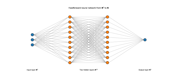
Figure 1: Illustration of (deep) neural network architecture with $d=3,\ell=1$

From a mathematical point of view, a neural network can be written as

$$x\in\mathbb{R}^{d}\mapsto\Phi(x;\theta):=\psi\circ a_{I}^{\theta_{I}}\circ\phi_{q_{I-1}}\circ a_{I-1}^{\theta_{I-1}}\circ\ldots\circ\phi_{q_{1}}\circ a_{1}^{\theta_{1}}(x)\in\mathbb{R}^{\ell},$$ (2.14)

where

$\rhd$ $I$ is the number of hidden layers representing the depth of the neural network.

$\rhd$ Each layer has weights $\mathcal{W}$ and bias $b$. For all $2\leq i\leq I$,

$$x\in\mathbb{R}^{q_{i-1}}\mapsto a_{i}^{\theta_{i}}(x)=\mathcal{W}_{i}\cdot x+b_{i}\in\mathbb{R}^{q_{i}}\hskip 17.07182pt\text{with}\hskip 11.38092pt\theta_{i}=(\mathcal{W}_{i},b_{i})\in\mathbb{R}^{q_{i-1}\times q_{i}}\times\mathbb{R}^{q_{i}},$$

and

$$x\in\mathbb{R}^{d}\mapsto a_{1}^{\theta_{1}}(x)=\mathcal{W}_{1}\cdot x+b_{1}\in\mathbb{R}^{q_{1}}\hskip 17.07182pt\text{with}\hskip 11.38092pt\theta_{1}=(\mathcal{W}_{1},b_{1})\in\mathbb{R}^{d\times q_{1}}\times\mathbb{R}^{q_{1}}.$$

$\rhd$ $q_{1},\ldots,q_{I}$ are positive integers denoting the number of nodes per hidden layer and representing the width of the neural network.

$\rhd$ $(\phi_{q_{i}})_{1\leq i\leq I-1}$ are non-linear functions called activation functions and are applied component wise.

$\rhd$ $\psi$ is the activation function for the output layer.

For the sake of simpler notation, we embed all the parameters of the different layers in a unique high dimensional parameter $\theta=\big{(}\theta_{1},\ldots,\theta_{I}\big{)}\in\mathbb{R}^{N_{q}}$ with $N_{q}=\sum_{i=1}^{I}q_{i-1}\cdot(1+q_{i})$ (with $q_{0}=d$). In order to study neural network approximation, we take the same notations as in [28]. We denote by $\mathcal{NN}_{\infty}$ the set of all neural networks of form (2.14). Then we consider, for some integer $m\geq 1$, $\mathcal{NN}_{m}$ the set of neural networks of form (2.14) with at most $m$ nodes per hidden layer and bounded parameters. More precisely, we consider

$$\Theta_{m}=\Big{\{}\mathbb{R}^{d}\times\mathbb{R}^{m}\times\big{(}\mathbb{R}^{m}\times\mathbb{R}^{m}\big{)}^{I-2}\times\mathbb{R}^{m}\times\mathbb{R}\hskip 5.69046pt:\hskip 5.69046pt|\theta|\leq\gamma_{m}\Big{\}}$$ (2.15)

which denotes the set of all parameters (bounded by $\gamma_{m}$) of a neural network with at most $m$ nodes per hidden layer. $(\gamma_{m})_{m\geq 2}$ is an increasing and non-bounded (real) sequence. Thus $\mathcal{NN}_{m}$ is defined as the set of all neural networks which parameters lie in $\Theta_{m}$,

$$\mathcal{NN}_{m}=\big{\{}\Phi(\cdot;\theta):\mathbb{R}^{d}\to\mathbb{R};\theta\in\Theta_{m}\big{\}}.$$ (2.16)

Note that $\displaystyle\mathcal{NN}_{\infty}=\bigcup_{m\in\mathbb{N}}\mathcal{NN}_{m}$.

In this paper, we consider the approximation of the continuation value using neural network. This leads to an approximated value function $V_{k}^{m}$ backwardly defined by

$$\left\{\begin{array}[]{ll}V_{k}^{m}\big{(}X_{t_{k}},Q\big{)}=\displaystyle\operatorname*{ess\,sup}_{q\in Adm(t_{k},Q)}\hskip 2.84544pt\psi\big{(}q,X_{t_{k}}\big{)}+\Phi_{m}\big{(}X_{t_{k}};\theta_{k+1,m}(Q+q)\big{)},\\ V_{n-1}^{m}\big{(}X_{t_{n-1}},Q\big{)}=V_{n-1}\big{(}X_{t_{n-1}},Q\big{)},\end{array}\right.$$ (2.17)

where $\Phi_{m}(\cdot;\theta)$ denotes a function lying within $\mathcal{NN}_{m}$ with $\theta\in\Theta_{m}$. Thus $\theta_{k+1,m}(Q)$ belongs to the following set

$$\mathcal{S}_{k}^{m}(Q):=\operatorname*{arg\,inf}_{\theta\in\Theta_{m}}\hskip 2.84544pt\Big{|}\Big{|}V_{k+1}^{m}(X_{t_{k+1}},Q)-\Phi_{m}\big{(}X_{t_{k}};\theta\big{)}\Big{|}\Big{|}_{2}.$$ (2.18)

To analyze the convergence of the neural network approximation we will rely on their powerful approximation ability. The latter is stated by the Universal Approximation Theorem.

Theorem 2.2 (Universal Approximation Theorem).

Assume that the activation functions in (2.14) are not constant and bounded. Let $\mu$ denote a probability measure on $\mathbb{R}^{d}$, then for any $I\geq 2$, $\mathcal{NN}_{\infty}$ is dense in $\mathbb{L}(\mathbb{R}^{d},\mu)$.

Remark 2.3.

As stated in [28], Theorem 2.2 can be seen as follows. For any (real) squared-integrable random variable $Y$ defined on a measurable space, there exists a sequence $\displaystyle(\theta_{m})_{m\geq 2}\in\prod_{m=2}^{\infty}\Theta_{m}$ such that $\displaystyle\lim_{p\to\infty}\big{|}\big{|}Y-\Phi_{m}(X;\theta)\big{|}\big{|}_{2}$ for some $\mathbb{R}^{d}$-valued random vector $X$. Thus, if for all $m\geq 2$, $\theta_{m}$ solves

$$\underset{\theta\in\Theta_{m}}{\inf}\hskip 2.84544pt\big{|}\big{|}\Phi_{m}(X;\theta)-Y\big{|}\big{|}_{2},$$

then the sequence $\big{(}\Phi_{m}(X;\theta_{m})\big{)}_{m\geq 2}$ converges to $\mathbb{E}(Y\rvert X)$ in $\mathbb{L}^{2}(\mu)$.

The universal approximation capacity of neural networks had been widely studied in the literature [25, 23, 16]. Some quantitative error bounds have been proved when the function to approximate is sufficiently smooth. A brief overview is presented in the following remark.

Remark 2.4 (UAT error bounds).

When the weighted average of the Fourier representation of the function to approximate is bounded, an error bound of the convergence in Remark 2.3 of order $\mathcal{O}(m^{-1/2})$ had been shown in [3, 4]. It may appears that the dimension of the problem does not degrade the convergence rate but as discussed by the authors, this may be hidden in the Fourier representation. In [2] it has been proved that, when the activation functions are infinitely continuously differentiables and the function to approximate is $p$-times continuously differentiable and Lipschitz, then the sup-norm of the approximation error on every compact set is bounded by a term of order $\mathcal{O}\big{(}m^{-(p+1)/d}\big{)}$. For a more detailed overview on quantitative error bounds, we refer the reader to [17].

Note that, as in the least squares method, in practice, we simulate $N$ independent paths $\big{(}X_{t_{0}}^{[p]},...,X_{t_{n-1}}^{[p]}\big{)}_{1\leq p\leq N}$ and use Monte Carlo approximation to compute the swing value function. For that purpose, we backwardly define the value function $V_{k}^{m,N}$ by,

$$\left\{\begin{array}[]{ll}V_{k}^{m,N}\big{(}X_{t_{k}}^{[p]},Q\big{)}=\displaystyle\operatorname*{ess\,sup}_{q\in Adm(t_{k},Q)}\hskip 2.84544pt\psi\big{(}q,X_{t_{k}}^{[p]}\big{)}+\Phi_{m}\big{(}X_{t_{k}}^{[p]};\theta_{k+1,m,N}(Q+q)\big{)},\\ V_{n-1}^{m,N}\big{(}X_{t_{n-1}}^{[p]},Q\big{)}=V_{n-1}\big{(}X_{t_{n-1}}^{[p]},Q\big{)},\end{array}\right.$$ (2.19)

where $\theta_{k+1,m,N}(Q)$ lies within the following set,

$$\mathcal{S}_{k}^{m,N}(Q):=\operatorname*{arg\,inf}_{\theta\in\Theta_{m}}\hskip 2.84544pt\frac{1}{N}\sum_{p=1}^{N}\Big{|}V_{k+1}^{m,N}(X_{t_{k+1}}^{[p]},Q)-\Phi_{m}\big{(}X_{t_{k}}^{[p]};\theta\big{)}\Big{|}^{2}.$$ (2.20)

Note that sets $\mathcal{S}_{k}^{m}(Q)$ or $\mathcal{S}_{k}^{m,N}(Q)$ (respectively defined in equations (2.18) and (2.20)) generally does not reduces to a singleton. Thus hereafter, the notation $\theta_{k+1,m}(Q)$ or $\theta_{k+1,m,N}(Q)$ will denote an element of the corresponding set $\mathcal{S}_{k}^{m}(Q)$ or $\mathcal{S}_{k}^{m,N}(Q)$.

3 Convergence analysis

We conduct a convergence analysis by following a similar approach as in [14, 28, 19]. Our initial focus is to establish a convergence result as the “architecture” used to approximate the continuation value increases. By architecture, we mean either regression functions (in the context of least squares approximation) or neural networks units per layer. Then, we fix the value of $m$ (representing the architecture’s size) and examine the associated Monte Carlo approximation. Let us start with the first step.

3.1 Convergence with respect to the number of approximation functions

We focus on the approximations (2.6) and (2.17) of the BDPP (1.7). In this section, we do not restrict ourselves to the bang-bang setting. That is, for both approximation methods, we consider arbitrary volume constraints (not limited to integers).

3.1.1 Least squares approximation

We start by analyzing the first approximation in the least squares setting (2.6). We show the convergence of the approximated value function $V_{k}^{m}$ as $m$ tends to infinity. To state this property we need the following result.

Proposition 3.1.

Let $m$ be a positive integer. Assume $\bm{\mathcal{H}_{2}^{LS}}$ and $\bm{\mathcal{H}_{3,2}}$ hold true. Then, for all $k=0,\ldots,n-2$, the function

$$Q\mapsto\big{|}\big{|}\Phi_{m}(X_{t_{k}};\tilde{\theta}_{k+1,m}(Q))-\mathbb{E}(V_{k+1}(X_{t_{k+1}},Q)\rvert X_{t_{k}})\big{|}\big{|}_{2}$$

is continuous on $\mathcal{T}_{k+1}$, where $\Phi_{m}$ is defined in (2.7) and $\tilde{\theta}_{k+1,m}(Q)$ solves the “theoretical” optimization problem

$$\underset{\theta\in\Theta_{m}}{\inf}\hskip 2.84544pt\Big{|}\Big{|}V_{k+1}\big{(}X_{t_{k+1}},Q\big{)}-\Phi_{m}(X_{t_{k}};\theta)\Big{|}\Big{|}_{2}.$$ (3.1)

Proof.

Keeping in mind relation (2), it suffices to prove that the functions,

$$Q\mapsto\big{|}\big{|}V_{k+1}(X_{t_{k+1}},Q)-\mathbb{E}(V_{k+1}(X_{t_{k+1}},Q)\rvert X_{t_{k}})\big{|}\big{|}_{2}^{2}$$ (3.2)

and

$$Q\mapsto\big{|}\big{|}V_{k+1}(X_{t_{k+1}},Q)-\Phi_{m}(X_{t_{k}};\tilde{\theta}_{k+1,m}(Q))\big{|}\big{|}_{2}^{2}$$ (3.3)

are continuous. Let us start with the first function. Let $Q\in\mathcal{T}_{k+1}$ and consider a sequence $\big{(}Q_{n}\big{)}_{n}$ which converges to $Q$. We know (as pointed out in Remark 2.1) that assumption $\bm{\mathcal{H}_{3,2}}$ entails that $V_{k+1}(X_{t_{k+1}},\cdot)$ is continuous and there exists $G_{k+1}\in\mathbb{L}_{\mathbb{R}}^{2}\big{(}\mathbb{P}\big{)}$ (independent of $Q$) such that $V_{k+1}(X_{t_{k+1}},\cdot)\leq G_{k+1}$. Thus the Lebesgue dominated convergence theorem implies that,

$$\lim\limits_{n\rightarrow+\infty}\hskip 2.84544pt\big{|}\big{|}V_{k+1}(X_{t_{k+1}},Q_{n})-\mathbb{E}(V_{k+1}(X_{t_{k+1}},Q_{n})\rvert X_{t_{k}})\big{|}\big{|}_{2}^{2}=\big{|}\big{|}V_{k+1}(X_{t_{k+1}},Q)-\mathbb{E}(V_{k+1}(X_{t_{k+1}},Q)\rvert X_{t_{k}})\big{|}\big{|}_{2}^{2}$$

yielding the continuity of the function defined in (3.2). We now prove the continuity of the second function defined in (3.3). Using assumption $\bm{\mathcal{H}_{2}^{LS}}$, it follows from Proposition A.3 that,

$$\Big{|}\Big{|}\Phi_{m}(X_{t_{k}};\tilde{\theta}_{k+1,m}(Q))-V_{k+1}(X_{t_{k+1}},Q)\Big{|}\Big{|}_{2}^{2}=\frac{G\big{(}V_{k+1}(X_{t_{k+1}},Q),e_{1}(X_{t_{k}}),\ldots,e_{m}(X_{t_{k}})\big{)}}{G\big{(}e_{1}(X_{t_{k}}),\ldots,e_{m}(X_{t_{k}})\big{)}}$$

where $G(x_{1},\ldots,x_{n})$ denotes the Gram determinant associated to the canonical $\mathbb{L}^{2}\big{(}\mathbb{P}\big{)}$ inner product. Since assumption $\bm{\mathcal{H}_{3,2}}$ entails the continuity of $V_{k+1}(X_{t_{k+1}},\cdot)$, then owing to the continuity of the determinant, one may conclude that $Q\in\mathcal{T}_{k+1}\mapsto\Big{|}\Big{|}\Phi_{m}(X_{t_{k}};\tilde{\theta}_{k+1,m}(Q))-V_{k+1}(X_{t_{k+1}},Q)\Big{|}\Big{|}_{2}^{2}$ is continuous as a composition of continuous functions. This completes the proof.

∎

The preceding proposition allows us to show our first convergence result stated in the following proposition.

Proposition 3.2.

Under assumptions $\bm{\mathcal{H}_{1}^{LS}}$, $\bm{\mathcal{H}_{2}^{LS}}$ and $\bm{\mathcal{H}_{3,2}}$, we have for all $0\leq k\leq n-1$,

$$\lim\limits_{m\rightarrow+\infty}\hskip 2.84544pt\underset{Q\in\mathcal{T}_{k}}{\sup}\hskip 2.84544pt\Big{|}\Big{|}V^{m}_{k}(X_{t_{k}},Q)-V_{k}(X_{t_{k}},Q)\Big{|}\Big{|}_{2}=0.$$

Proof.

We proceed by a backward induction on $k$. We have, almost surely, $V^{m}_{n-1}(X_{t_{n-1}},Q)=V_{n-1}(X_{t_{n-1}},Q)$ for any $Q\in\mathcal{T}_{n-1}$ and therefore the proposition holds true for $k=n-1$. Let us suppose it holds for $k+1$. For all $Q\in\mathcal{T}_{k}$ using the inequality $|\underset{i\in I}{\sup}\hskip 2.84544pta_{i}-\underset{i\in I}{\sup}\hskip 2.84544ptb_{i}|\hskip 2.84544pt\leq\hskip 2.84544pt\underset{i\in I}{\sup}\hskip 2.84544pt|a_{i}-b_{i}|$, we get,

$$\big{|}V^{m}_{k}(X_{t_{k}},Q)-V_{k}(X_{t_{k}},Q)\big{|}^{2} \leq\operatorname*{ess\,sup}_{q\in Adm(t_{k},Q)}\big{|}\Phi_{m}(X_{t_{k}};\theta_{k+1,m}(Q+q))-\mathbb{E}(V_{k+1}(X_{t_{k+1}},Q+q)\rvert X_{t_{k}})\big{|}^{2}.$$

Taking the expectation in the previous inequality yields,

$$\big{|}\big{|}V^{m}_{k}(X_{t_{k}},Q)-V_{k}(X_{t_{k}},Q)\big{|}\big{|}_{2}^{2} \leq\mathbb{E}\left(\operatorname*{ess\,sup}_{q\in Adm(t_{k},Q)}\Big{|}\Phi_{m}(X_{t_{k}};\theta_{k+1,m}(Q+q))-\mathbb{E}(V_{k+1}(X_{t_{k+1}},Q+q)\rvert X_{t_{k}})\Big{|}^{2}\right).$$ (3.4)

To interchange the essential supremum with the expectation, we rely on the bifurcation property. For all $q\in Adm(t_{k},Q)$, consider

$$A_{k}^{m}(Q,q):=\Big{|}\Phi_{m}(X_{t_{k}};\theta_{k+1,m}(Q+q))-\mathbb{E}(V_{k+1}(X_{t_{k+1}},Q+q)\rvert X_{t_{k}})\Big{|}^{2}.$$

Then for all $q_{1},q_{2}\in Adm(t_{k},Q)$ define the following random variable

$$q_{A}^{*}=q_{1}\cdot\mathrm{1}_{\{A_{k}^{m}(Q,q_{1})\geq A_{k}^{m}(Q,q_{2})\}}+q_{2}\cdot\mathrm{1}_{\{A_{k}^{m}(Q,q_{1})<A_{k}^{m}(Q,q_{2})\}}.$$ (3.5)

It follows from the definition of $\Phi_{m}$ in (2.7) and that of the conditional expectation that $A_{k}^{m}(Q,q)$ is $\sigma\left(X_{t_{k}}\right)$-measurable for all $q\in Adm(t_{k},Q)$. Thus using (3.5) yields $q_{A}^{*}\in Adm(t_{k},Q)$ and $A_{k}^{m}(Q,q_{A}^{*})=\max\left(A_{k}^{m}(Q,q_{1}),A_{k}^{m}(Q,q_{2})\right)$. Therefore one may use the bifurcation property in (3.4) and we get,

$$\big{|}\big{|}V^{m}_{k}(X_{t_{k}},Q)-V_{k}(X_{t_{k}},Q)\big{|}\big{|}_{2}^{2} \leq\underset{q\in Adm(t_{k},Q)}{\sup}\big{|}\big{|}\Phi_{m}(X_{t_{k}};\theta_{k+1,m}(Q+q))-\mathbb{E}(V_{k+1}(X_{t_{k+1}},Q+q)\rvert X_{t_{k}})\big{|}\big{|}_{2}^{2}$$

$$\leq 2\underset{q\in Adm(t_{k},Q)}{\sup}\big{|}\big{|}\Phi_{m}(X_{t_{k}};\theta_{k+1,m}(Q+q))-\Phi_{m}(X_{t_{k}};\tilde{\theta}_{k+1,m}(Q+q))\big{|}\big{|}_{2}^{2}$$

$$+2\underset{q\in Adm(t_{k},Q)}{\sup}\big{|}\big{|}\Phi_{m}(X_{t_{k}};\tilde{\theta}_{k+1,m}(Q+q))-\mathbb{E}(V_{k+1}(X_{t_{k+1}},Q+q)\rvert X_{t_{k}})\big{|}\big{|}_{2}^{2}$$ (3.6)

where in the last inequality, we used Minkowski inequality. $\tilde{\theta}_{k+1,m}(Q+q)$ solves the “theoretical” optimization problem (3.1). Note that in the latter problem, we introduced the actual (not known) value function $V_{k+1}$ unlike in equation (2.8). This is just a theoretical tool as the preceding optimization problem cannot be solved since we do not know the actual value function $V_{k+1}$. Thus taking the supremum in (3.1.1) yields,

$$\underset{Q\in\mathcal{T}_{k}}{\sup}\big{|}\big{|}V^{m}_{k}(X_{t_{k}},Q)-V_{k}(X_{t_{k}},Q)\big{|}\big{|}_{2}^{2}$$

$$\leq 2\underset{Q\in\mathcal{T}_{k+1}}{\sup}\big{|}\big{|}\Phi_{m}(X_{t_{k}};\theta_{k+1,m}(Q))-\Phi_{m}(X_{t_{k}};\tilde{\theta}_{k+1,m}(Q))\big{|}\big{|}_{2}^{2}$$

$$+2\underset{Q\in\mathcal{T}_{k+1}}{\sup}\big{|}\big{|}\Phi_{m}(X_{t_{k}};\tilde{\theta}_{k+1,m}(Q))-\mathbb{E}(V_{k+1}(X_{t_{k+1}},Q)\rvert X_{t_{k}})\big{|}\big{|}_{2}^{2},$$ (3.7)

where we used the fact that, for all $Q\in\mathcal{T}_{k}$ and all $q\in Adm(t_{k},Q)$ we have $Q+q\in\mathcal{T}_{k+1}$. Besides, recall that $\Phi_{m}(X_{t_{k}};\tilde{\theta}_{k+1,m}(Q))$ and $\Phi_{m}(X_{t_{k}};\theta_{k+1,m}(Q))$ are orthogonal projections of $V_{k+1}(X_{t_{k+1}},Q)$ and $V_{k+1}^{m}(X_{t_{k+1}},Q)$ on the subspace spanned by $e^{m}(X_{t_{k}})$. Then knowing that the orthogonal projection is 1-Lipschitz, we have

$$\underset{Q\in\mathcal{T}_{k+1}}{\sup}\big{|}\big{|}\Phi_{m}(X_{t_{k}};\theta_{k+1,m}(Q))-\Phi_{m}(X_{t_{k}};\tilde{\theta}_{k+1,m}(Q))\big{|}\big{|}_{2}^{2}\leq\underset{Q\in\mathcal{T}_{k+1}}{\sup}\big{|}\big{|}V^{m}_{k+1}(X_{t_{k+1}},Q)-V_{k+1}(X_{t_{k+1}},Q)\big{|}\big{|}_{2}^{2}.$$

Thanks to the induction assumption, the right hand side of the last inequality converges to $0$ as $m\to+\infty$, so that,

$$\underset{Q\in\mathcal{T}_{k+1}}{\sup}\big{|}\big{|}\Phi_{m}(X_{t_{k}};\theta_{k+1,m}(Q))-\Phi_{m}(X_{t_{k}};\tilde{\theta}_{k+1,m}(Q))\big{|}\big{|}_{2}^{2}\hskip 5.69046pt\xrightarrow[m\to+\infty]{}0.$$ (3.8)

It remains to prove that

$$\lim\limits_{m\rightarrow+\infty}\hskip 2.84544pt\underset{Q\in\mathcal{T}_{k+1}}{\sup}\Big{|}\Big{|}\Phi_{m}(X_{t_{k}};\tilde{\theta}_{k+1,m}(Q))-\mathbb{E}(V_{k+1}(X_{t_{k+1}},Q)\rvert X_{t_{k}})\Big{|}\Big{|}_{2}^{2}=0.$$ (3.9)

To achieve, this we rely on Dini’s lemma whose assumptions hold true owing to the three following facts.

Pointwise convergence

It follows from assumption $\bm{\mathcal{H}_{1}^{LS}}$ that, for any $Q\in\mathcal{T}_{k+1}$,

$$\lim\limits_{m\rightarrow+\infty}\Big{|}\Big{|}\Phi_{m}(X_{t_{k}};\tilde{\theta}_{k+1,m}(Q))-\mathbb{E}(V_{k+1}(X_{t_{k+1}},Q)\rvert X_{t_{k}})\Big{|}\Big{|}_{2}^{2}=0.$$

Continuity

The continuity of $Q\mapsto\Big{|}\Big{|}\Phi_{m}(X_{t_{k}};\tilde{\theta}_{k+1,m}(Q))-\mathbb{E}(V_{k+1}(X_{t_{k+1}},Q)\rvert X_{t_{k}})\Big{|}\Big{|}_{2}^{2}$ is given by Proposition 3.1 under assumptions $\bm{\mathcal{H}_{2}^{LS}}$ and $\bm{\mathcal{H}_{3,2}}$.

Monotony

Denote by $F_{m}^{k}:=\operatorname{span}\big{(}e_{1}(X_{t_{k}}),\ldots,e_{m}(X_{t_{k}})\big{)}$. Then it is straightforward that for any $m\geq 1$, $F_{m}^{k}\subseteq F_{m+1}^{k}$. So that,

$$\Big{|}\Big{|}\Phi_{m}(X_{t_{k}};\tilde{\theta}_{k+1,m}(Q))-\mathbb{E}(V_{k+1}(X_{t_{k+1}},Q)\rvert X_{t_{k}})\Big{|}\Big{|}_{2}^{2} =\underset{Y\in F_{m}^{k}}{\inf}\hskip 2.84544pt\Big{|}\Big{|}\mathbb{E}\big{(}V_{k+1}(X_{t_{k+1}},Q)\rvert X_{t_{k}}\big{)}-Y\Big{|}\Big{|}_{2}^{2}$$

$$\geq\underset{Y\in F_{m+1}^{k}}{\inf}\hskip 2.84544pt\Big{|}\Big{|}\mathbb{E}\big{(}V_{k+1}(X_{t_{k+1}},Q)\rvert X_{t_{k}}\big{)}-Y\Big{|}\Big{|}_{2}^{2}$$

$$=\Big{|}\Big{|}\Phi_{m+1}(X_{t_{k}};\tilde{\theta}_{k+1,m+1}(Q))-\mathbb{E}(V_{k+1}(X_{t_{k+1}},Q)\rvert X_{t_{k}})\Big{|}\Big{|}_{2}^{2}.$$

Thus the sequence,

$$\left(\Big{|}\Big{|}\Phi_{m}(X_{t_{k}};\tilde{\theta}_{k+1,m}(Q))-\mathbb{E}(V_{k+1}(X_{t_{k+1}},Q)\rvert X_{t_{k}})\Big{|}\Big{|}_{2}^{2}\right)_{m\geq 1}$$

is non-increasing. From the three preceding properties, one may apply Dini lemma yielding the desired result (3.9). Finally, combining (3.8) and (3.9) in (3.1.1) yields,

$$\lim\limits_{m\rightarrow+\infty}\hskip 2.84544pt\underset{Q\in\mathcal{T}_{k}}{\sup}\big{|}\big{|}V^{m}_{k}(X_{t_{k}},Q)-V_{k}(X_{t_{k}},Q)\big{|}\big{|}_{2}^{2}=0.$$

This completes the proof.

∎

3.1.2 Neural network approximation

We now consider the approximation of the continuation value when using neural network. We prove a similar result as in Proposition 3.2, when the number of units per hidden layer increases. To achieve this, we need the following assumptions.

$\bm{\mathcal{H}_{1}^{\mathcal{NN}}}$: For every $m\geq 2$, there exists $q\geq 1$ such that for every $\theta\in\Theta_{m}$, $\Phi_{m}(\cdot;\theta)$ has $q$-polynomial growth uniformly in $\theta$.

$\bm{\mathcal{H}_{2}^{\mathcal{NN}}}$: For any $0\leq k\leq n-1$, a.s. the random functions $\theta\in\Theta_{m}\mapsto\Phi_{m}\big{(}X_{t_{k}};\theta\big{)}$ are continuous. Owing to the Heine theorem, the compactness of $\Theta_{m}$ yields the uniform continuity.

Proposition 3.3.

Assume $\bm{\mathcal{H}_{1}^{\mathcal{NN}}}$, $\bm{\mathcal{H}_{2}^{\mathcal{NN}}}$ and $\bm{\mathcal{H}_{3,2q}}$ (with $q$ involved in assumption $\bm{\mathcal{H}_{1}^{\mathcal{NN}}}$) hold true. Then, for all $0\leq k\leq n-1$,

$$\lim\limits_{m\rightarrow+\infty}\hskip 2.84544pt\underset{Q\in\mathcal{T}_{k}}{\sup}\hskip 2.84544pt\Big{|}\Big{|}V^{m}_{k}(X_{t_{k}},Q)-V_{k}(X_{t_{k}},Q)\Big{|}\Big{|}_{2}=0.$$

Proof.

We proceed by a backward induction on $k$. For $k=n-1$, we have $V^{m}_{n-1}(X_{t_{n-1}},Q)=V_{n-1}(X_{t_{n-1}},Q)$ and therefore the proposition holds true. Let us suppose it holds for $k+1$. In the spirit of the beginning of the proof of Proposition 3.2, we have for all $Q\in\mathcal{T}_{k}$ using the inequality: $|\underset{i\in I}{\sup}\hskip 2.84544pta_{i}-\underset{i\in I}{\sup}\hskip 2.84544ptb_{i}|\hskip 2.84544pt\leq\hskip 2.84544pt\underset{i\in I}{\sup}\hskip 2.84544pt|a_{i}-b_{i}|$ and triangle inequality,

$$\big{|}\big{|}V^{m}_{k}(X_{t_{k}},Q)-V_{k}(X_{t_{k}},Q)\big{|}\big{|}_{2}^{2} \leq\mathbb{E}\left(\operatorname*{ess\,sup}_{q\in Adm(t_{k},Q)}\left|\Phi_{m}\big{(}X_{t_{k}};\theta_{k+1,m}(Q+q)\big{)}-\mathbb{E}\big{(}V_{k+1}(X_{t_{k+1}},Q+q)\rvert X_{t_{k}}\big{)}\right|^{2}\right).$$ (3.10)

Then we aim to apply the bifurcation property. For all $q\in Adm(t_{k},Q)$, consider,

$$A_{k}^{m}(Q,q)=\Big{|}\Phi_{m}\big{(}X_{t_{k}};\theta_{k+1,m}(Q+q)\big{)}-\mathbb{E}\big{(}V_{k+1}(X_{t_{k+1}},Q+q)\rvert X_{t_{k}}\big{)}\Big{|}^{2}.$$

Then for all $q_{1},q_{2}\in Adm(t_{k},Q)$ define

$$q_{A}^{*}=q_{1}\cdot\mathrm{1}_{\{A_{k}^{m}(Q,q_{1})\geq A_{k}^{m}(Q,q_{2})\}}+q_{2}\cdot\mathrm{1}_{\{A_{k}^{m}(Q,q_{1})<A_{k}^{m}(Q,q_{2})\}}.$$

Using the definition of the conditional expectation and since activation functions are continuous (assumption $\bm{\mathcal{H}_{2}^{\mathcal{NN}}}$), $A_{k}^{m}(Q,q)$ is $\sigma\left(X_{t_{k}}\right)$-measurable for all $q\in Adm(t_{k},Q)$. Moreover, $q_{A}^{*}\in Adm(t_{k},Q)$ and $A_{k}^{m}(Q,q_{A}^{*})=\max\left(A_{k}^{m}(Q,q_{1}),A_{k}^{m}(Q,q_{2})\right)$. Thus using the bifurcation property and taking the supremum in (3.10) yields,

$$\underset{Q\in\mathcal{T}_{k}}{\sup}\big{|}\big{|}V^{m}_{k}(X_{t_{k}},Q)-V_{k}(X_{t_{k}},Q)\big{|}\big{|}_{2}^{2}\leq\underset{Q\in\mathcal{T}_{k+1}}{\sup}\big{|}\big{|}\Phi_{m}\big{(}X_{t_{k}};\theta_{k+1,m}(Q)\big{)}-\mathbb{E}\big{(}V_{k+1}(X_{t_{k+1}},Q)\rvert X_{t_{k}}\big{)}\big{|}\big{|}_{2}^{2}.$$

Using Minkowski inequality and the inequality: $(a+b)^{2}\leq 2(a^{2}+b^{2})$ yields,

$$\underset{Q\in\mathcal{T}_{k}}{\sup}\big{|}\big{|}V^{m}_{k}(X_{t_{k}},Q)-V_{k}(X_{t_{k}},Q)\big{|}\big{|}_{2}^{2} \leq 2\underset{Q\in\mathcal{T}_{k+1}}{\sup}\big{|}\big{|}\mathbb{E}\big{(}V_{k+1}^{m}(X_{t_{k+1}},Q)\rvert X_{t_{k}}\big{)}-\mathbb{E}\big{(}V_{k+1}(X_{t_{k+1}},Q)\rvert X_{t_{k}}\big{)}\big{|}\big{|}_{2}^{2}$$

$$+2\underset{Q\in\mathcal{T}_{k+1}}{\sup}\big{|}\big{|}\Phi_{m}\big{(}X_{t_{k}};\theta_{k+1,m}(Q)\big{)}-\mathbb{E}\big{(}V_{k+1}^{m}(X_{t_{k+1}},Q)\rvert X_{t_{k}}\big{)}\big{|}\big{|}_{2}^{2}.$$

By the induction assumption, the first term in the right hand side converges to $0$ as $m\to+\infty$. Let us consider the second term. Since $\theta_{k+1,m}(Q)$ solves (2.18), we have

$$\underset{Q\in\mathcal{T}_{k+1}}{\sup}\big{|}\big{|}\Phi_{m}\big{(}X_{t_{k}};\theta_{k+1,m}(Q)\big{)}-\mathbb{E}\big{(}V_{k+1}^{m}(X_{t_{k+1}},Q)\rvert X_{t_{k}}\big{)}\big{|}\big{|}_{2}^{2}\leq\underset{Q\in\mathcal{T}_{k+1}}{\sup}\big{|}\big{|}\Phi_{m}\big{(}X_{t_{k}};\tilde{\theta}_{k+1,m}(Q)\big{)}-\mathbb{E}\big{(}V_{k+1}^{m}(X_{t_{k+1}},Q)\rvert X_{t_{k}}\big{)}\big{|}\big{|}_{2}^{2},$$

where $\tilde{\theta}_{k+1,m}(Q)$ solves the “theoretical” optimization problem,

$$\underset{\theta\in\Theta_{m}}{\inf}\hskip 2.84544pt\Big{|}\Big{|}V_{k+1}\big{(}X_{t_{k+1}},Q\big{)}-\Phi_{m}\big{(}X_{t_{k}};\theta\big{)}\Big{|}\Big{|}_{2}$$

with $\Theta_{m}$ defined in (2.15). Then it follows from Minskowki inequality that

$$\underset{Q\in\mathcal{T}_{k+1}}{\sup}\big{|}\big{|}\Phi_{m}\big{(}X_{t_{k}};\tilde{\theta}_{k+1,m}(Q)\big{)}-\mathbb{E}\big{(}V_{k+1}^{m}(X_{t_{k+1}},Q)\rvert X_{t_{k}}\big{)}\big{|}\big{|}_{2}^{2} \leq\underset{Q\in\mathcal{T}_{k+1}}{\sup}\big{|}\big{|}\mathbb{E}\big{(}V_{k+1}(X_{t_{k+1}},Q)\rvert X_{t_{k}}\big{)}-\mathbb{E}\big{(}V_{k+1}^{m}(X_{t_{k+1}},Q)\rvert X_{t_{k}}\big{)}\big{|}\big{|}_{2}^{2}$$

$$+\underset{Q\in\mathcal{T}_{k+1}}{\sup}\big{|}\big{|}\Phi_{m}\big{(}X_{t_{k}};\tilde{\theta}_{k+1,m}(Q)\big{)}-\mathbb{E}\big{(}V_{k+1}(X_{t_{k+1}},Q)\rvert X_{t_{k}}\big{)}\big{|}\big{|}_{2}^{2}.$$

Once again, by the induction assumption, the first term in the right hand side converges to $0$ as $m\to+\infty$. Moreover, thanks to the universal approximation theorem, for all $Q\in\mathcal{T}_{k+1}$

$$\big{|}\big{|}\Phi_{m}\big{(}X_{t_{k}};\tilde{\theta}_{k+1,m}(Q)\big{)}-\mathbb{E}\big{(}V_{k+1}(X_{t_{k+1}},Q)\rvert X_{t_{k}}\big{)}\big{|}\big{|}_{2}^{2}\xrightarrow[m\to+\infty]{}0.$$ (3.11)

Besides notice that,

$$\big{|}\big{|}\Phi_{m}\big{(}X_{t_{k}};\tilde{\theta}_{k+1,m}(Q)\big{)}-\mathbb{E}\big{(}V_{k+1}(X_{t_{k+1}},Q)\rvert X_{t_{k}}\big{)}\big{|}\big{|}_{2}^{2} =\underset{\Phi\in\mathcal{NN}_{m}}{\inf}\big{|}\big{|}\Phi\big{(}X_{t_{k}}\big{)}-\mathbb{E}\big{(}V_{k+1}(X_{t_{k+1}},Q)\rvert X_{t_{k}}\big{)}\big{|}\big{|}_{2}^{2}$$ (3.12)

where $\mathcal{NN}_{m}$ is defined in (2.16). But since the sequence $\big{(}\Theta_{m}\big{)}_{m}$ is non-decreasing (in the sense that $\Theta_{m}\subseteq\Theta_{m+1}$), then $\big{(}\mathcal{NN}_{m}\big{)}_{m}$ is too. So that by the previous equality (3.12),

$$\Big{(}\big{|}\big{|}\Phi_{m}\big{(}X_{t_{k}};\tilde{\theta}_{k+1,m}(Q)\big{)}-\mathbb{E}\big{(}V_{k+1}(X_{t_{k+1}},Q)\rvert X_{t_{k}}\big{)}\big{|}\big{|}_{2}^{2}\Big{)}_{m\geq 2}$$

is a non-increasing sequence. Thus keeping in mind equation (3.12), if the function,

$$H_{k}\colon\big{(}\mathcal{NN}_{m},\hskip 2.84544pt|\cdot|_{\sup}\big{)}\times\big{(}\mathcal{T}_{k+1},\hskip 2.84544pt|\cdot|\big{)} \to\mathbb{R}$$

$$(\Phi,Q) \longmapsto||L_{k}(\Phi,Q)||_{2}^{2}:=\big{|}\big{|}\Phi\big{(}X_{t_{k}}\big{)}-\mathbb{E}\big{(}V_{k+1}(X_{t_{k+1}},Q)\rvert X_{t_{k}}\big{)}\big{|}\big{|}_{2}^{2}$$

is continuous, then thanks to Theorem A.2 (noticing that for all $m\geq 2$, $\mathcal{NN}_{m}$ is a compact set), the function

$$Q\mapsto\big{|}\big{|}\Phi_{m}\big{(}X_{t_{k}};\tilde{\theta}_{k+1,m}(Q)\big{)}-\mathbb{E}\big{(}V_{k+1}(X_{t_{k+1}},Q)\rvert X_{t_{k}}\big{)}\big{|}\big{|}_{2}^{2}$$

will be continuous on the compact set $\mathcal{T}_{k+1}$. Thus one may use Dini lemma and conclude that the pointwise convergence in (3.11) is in fact uniform. Which will completes the proof.

Note that we have already shown that $Q\mapsto\mathbb{E}\big{(}V_{k+1}(X_{t_{k+1}},Q)\rvert X_{t_{k}}\big{)}$ is almost surely continuous under assumption $\bm{\mathcal{H}_{3,2q}}$. Moreover using the classic inequality: $(a+b)^{2}\leq 2(a^{2}+b^{2})$ and then conditional Jensen inequality

$$\big{|}L_{k}(\Phi,Q)|^{2} \leq 2\cdot\big{|}\Phi\big{(}X_{t_{k}}\big{)}\big{|}^{2}+2\cdot\mathbb{E}\big{(}V_{k+1}(X_{t_{k+1}},Q)^{2}\rvert X_{t_{k}}\big{)}$$

$$\leq 2\cdot\big{|}\Phi\big{(}X_{t_{k}}\big{)}\big{|}^{2}+2\cdot\mathbb{E}\big{(}G_{k+1}^{2}\rvert X_{t_{k}}\big{)}\in\mathbb{L}^{1}_{\mathbb{R}}\big{(}\mathbb{P}\big{)},$$

where the existence of $G_{k+1}\in\mathbb{L}^{2}_{\mathbb{R}}(\mathbb{P})$ (independent of $Q$) follows from Remark 2.1 and is implied by assumption $\bm{\mathcal{H}_{3,2q}}$. Note that the integrability of $\big{|}\Phi\big{(}X_{t_{k}}\big{)}\big{|}^{2}$ follows from assumptions $\bm{\mathcal{H}_{1}^{\mathcal{NN}}}$ and $\bm{\mathcal{H}_{3,2q}}$. This implies that $||L_{k}(\Phi,\cdot)||_{2}^{2}$ is continuous.

Besides, for some sequence $(\Phi_{n})_{n}$ of $\mathcal{NN}_{m}$ such that $\Phi_{n}\xrightarrow[n\to+\infty]{|\cdot|_{\sup}}\Phi$, it follows from the Lebesgue’s dominated convergence theorem (enabled by assumptions $\bm{\mathcal{H}_{1}^{\mathcal{NN}}}$ and $\bm{\mathcal{H}_{3,2q}}$) that $||L_{k}(\Phi_{n},Q)||_{2}^{2}\xrightarrow[n\to+\infty]{}||L_{k}(\Phi,Q)||_{2}^{2}$. Which shows that $||L_{k}(\cdot,Q)||_{2}^{2}$ is continuous. Therefore the function $H_{k}$ is continuous. And as already mentioned this completes the proof.

∎

Remark 3.4 (Assumptions $\bm{\mathcal{H}_{1}^{\mathcal{NN}}}$ and $\bm{\mathcal{H}_{2}^{\mathcal{NN}}}$).

In the previous proposition, we made the assumption that the neural networks are continuous and with polynomial growth. This assumption is clearly satisfied when using classic activation functions such as the ReLU function $x\in\mathbb{R}\mapsto\max(x,0)$ and Sigmoïd function $x\in\mathbb{R}\mapsto 1/(1+e^{-x})$.

3.2 Convergence of Monte Carlo approximation

From now on, we assume a fixed positive integer $m$ and focus is on the convergence of the value function that arises from the second approximation (2.11) or (2.19). Unlike the preceding section and for technical convenience, we restrict our analysis of the neural network approximation to the bang-bang setting. However, the least squares regression will still be examined in a general context.

3.2.1 Least squares regression

We establish a convergence result under the following Hilbert assumption.

$\bm{\mathcal{H}_{5}^{LS}}$: For all $k=0,\ldots,n-1$ the sequence $\left(e_{i}\left(X_{t_{k}}\right)\right)_{i\geq 1}$ is a Hilbert basis of $\mathbb{L}^{2}\big{(}\sigma(X_{t_{k}})\big{)}$.

It is worth noting that this assumption is a special case of assumptions $\bm{\mathcal{H}_{1}^{LS}}$ and $\bm{\mathcal{H}_{2}^{LS}}$ with an orthonormality assumption on $e^{m}\big{(}X_{t_{k}}\big{)}$. Furthermore, in the field of mathematical finance, the underlying asset’s diffusion is often assumed to have a Gaussian structure. However, it is well known that the normalized Hermite polynomials $\big{\{}\frac{H_{k}(x)}{\sqrt{k!}},k\geq 0\big{\}}$ serve as a Hilbert basis for $\mathbb{L}^{2}(\mathbb{R},\mu)$, the space of square-integrable functions with respect to the Gaussian measure $\mu$. The Hermite polynomials $\big{\{}H_{k}(x),k\geq 0\big{\}}$ are defined as follows:

$$H_{k}(x)=(-1)^{k}e^{x^{2}}\frac{d^{k}}{dx^{k}}\big{[}e^{-x^{2}}\big{]},$$

or recursively by

$$H_{k+1}(x)=2x\cdot H_{k}(x)-2k\cdot H_{k-1}(x)\hskip 11.38092pt\text{with}\hskip 11.38092ptH_{0}(x)=1,\hskip 5.69046ptH_{1}(x)=2x.$$

For a multidimensional setting, Hermite polynomials are obtained as the product of one-dimensional Hermite polynomials. Finally, note that assumptions $\bm{\mathcal{H}_{5}^{LS}}$ entail that $A_{m}^{k}=A_{m,N}^{k}=I_{m}$.

The main result of this section aim at proving that the second approximation $V_{k}^{m,N}$ of the swing value function converges towards the first approximation $V_{k}^{m}$ as the Monte Carlo sample size $N$ increases to $+\infty$ and with a rate of convergence of order $\mathcal{O}\big{(}\frac{1}{\sqrt{N}}\big{)}$. To achieve this we rely on the following lemma which concern general Monte Carlo rate of convergence.

Lemma 3.5 (Monte Carlo $\mathbb{L}^{r}\big{(}\mathbb{P}\big{)}$-rate of convergence).

Consider $X_{1},\ldots,X_{N}$ independent and identically distributed random variables with order $p$ ($p\geq 2$) finite moment (with $\mu=\mathbb{E}(X_{1})$). Then, there exists a positive constant $B_{p}$ (only depending on the order $p$) such that

$$\Big{|}\Big{|}\frac{1}{N}\sum_{i=1}^{N}X_{i}-\mu\Big{|}\Big{|}_{p}\leq B_{p}\frac{2^{\frac{p-1}{p}}\Big{(}\mathbb{E}(|X|^{p})+|\mu|^{p}\Big{)}^{\frac{1}{p}}}{\sqrt{N}}.$$

Proof.

It follows from Marcinkiewicz–Zygmund inequality that there exists a positive constant $A_{p}$ (only depends on $p$) such that

$$\Big{|}\Big{|}\frac{1}{N}\sum_{i=1}^{N}X_{i}-\mu\Big{|}\Big{|}_{p}^{p}=\mathbb{E}\left(\Big{(}\sum_{i=1}^{N}\frac{X_{i}-\mu}{N}\Big{)}^{p}\right)\leq A_{p}\cdot\mathbb{E}\left(\Big{(}\frac{1}{N^{2}}\sum_{i=1}^{N}(X_{i}-\mu)^{2}\Big{)}^{p/2}\right)$$

$$=\frac{A_{p}}{N^{\frac{p}{2}}}\cdot\mathbb{E}\left(\Big{(}\frac{1}{N}\sum_{i=1}^{N}(X_{i}-\mu)^{2}\Big{)}^{p/2}\right).$$

Using the convexity of the function $x\in\mathbb{R}_{+}\mapsto x^{p/2}$ yields,

$$\Big{(}\frac{1}{N}\sum_{i=1}^{N}(X_{i}-\mu)^{2}\Big{)}^{p/2}\leq\frac{1}{N}\sum_{i=1}^{N}(X_{i}-\mu)^{p}.$$

Thus taking the expectation and using the inequality, $(a+b)^{p}\leq 2^{p-1}(a^{p}+b^{p})$ yields,

$$\left|\left|\frac{1}{N}\sum_{i=1}^{N}X_{i}-\mu\right|\right|_{p}^{p}\leq\frac{A_{p}}{N^{\frac{p}{2}}}\cdot\mathbb{E}\Big{(}(X-\mu)^{p}\Big{)}\leq A_{p}\cdot\frac{2^{p-1}\Big{(}\mathbb{E}(|X|^{p})+|\mu|^{p}\Big{)}}{N^{\frac{p}{2}}}.$$

This completes the proof.

∎

In the following proposition, we show that using Hilbert basis as a regression basis allows to achieve a convergence with a rate of order $\mathcal{O}(\frac{1}{\sqrt{N}})$.

Proposition 3.6.

Under assumptions $\bm{\mathcal{H}_{3,\infty}}$, $\bm{\mathcal{H}_{4,\infty}^{LS}}$ and $\bm{\mathcal{H}_{5}^{LS}}$, for all $k=0,\ldots,n-1$ and for any $s>1$, we have

$$\underset{Q\hskip 2.84544pt\in\hskip 2.84544pt\mathcal{T}_{k}}{\sup}\hskip 5.69046pt\left|\left|V^{m,N}_{k}\left(X_{t_{k}},Q\right)-V^{m}_{k}\left(X_{t_{k}},Q\right)\right|\right|_{s}=\mathcal{O}\left(\frac{1}{\sqrt{N}}\right)\hskip 14.22636pt\text{as}\hskip 5.69046ptN\to+\infty.$$

Proof.

We prove this proposition using a backward induction on $k$. Since $V^{m,N}_{n-1}\left(X_{t_{n-1}},\cdot\right)=V^{m}_{n-1}\left(X_{t_{n-1}},\cdot\right)$ on $\mathcal{T}_{n-1}$, then the proposition holds for $k=n-1$. Assume now that the proposition holds for $k+1$. Using the inequality, $|\underset{i\in I}{\sup}\hskip 2.84544pta_{i}-\underset{i\in I}{\sup}\hskip 2.84544ptb_{i}|\hskip 2.84544pt\leq\hskip 2.84544pt\underset{i\in I}{\sup}\hskip 2.84544pt|a_{i}-b_{i}|$ and then Cauchy-Schwartz’ one, we get,

$$\big{|}V^{m,N}_{k}\left(X_{t_{k}},Q\right)-V^{m}_{k}(X_{t_{k}},Q)\big{|} \leq\operatorname*{ess\,sup}_{q\in Adm(t_{k},Q)}\big{|}\langle\theta_{k+1,m,N}(Q+q)-\theta_{k+1,m}(Q+q),e^{m}(X_{t_{k}})\rangle\big{|}$$

$$\leq\big{|}e^{m}(X_{t_{k}})\big{|}\cdot\operatorname*{ess\,sup}_{q\in Adm(t_{k},Q)}\hskip 2.84544pt\big{|}\theta_{k+1,m,N}(Q+q)-\theta_{k+1,m}(Q+q)\big{|}$$

$$\leq\big{|}e^{m}(X_{t_{k}})\big{|}\cdot\operatorname*{ess\,sup}_{q\hskip 2.84544pt\in\hskip 2.84544pt\mathcal{U}_{k}(Q)}\hskip 2.84544pt\big{|}\theta_{k+1,m,N}(Q+q)-\theta_{k+1,m}(Q+q)\big{|},$$

where $\mathcal{U}_{k}(Q)$ is the set of all $\mathcal{F}_{t_{k+1}}^{X}$-measurable random variables lying within $\mathcal{I}_{k+1}\big{(}Q\big{)}$ (see (1.8)). The last inequality is due to the fact that $\mathcal{F}_{t_{k}}^{X}\subset\mathcal{F}_{t_{k+1}}^{X}$. Then for some constants $b,c>1$ such that $\frac{1}{b}+\frac{1}{c}=1$, it follows from Hölder inequality that,

$$\Big{|}\Big{|}V^{m,N}_{k}(X_{t_{k}},Q)-V^{m}_{k}(X_{t_{k}},Q)\Big{|}\Big{|}_{s} \leq\Big{|}\Big{|}|e^{m}(X_{t_{k}})|\Big{|}\Big{|}_{sb}\cdot\Big{|}\Big{|}\operatorname*{ess\,sup}_{q\hskip 2.84544pt\in\hskip 2.84544pt\mathcal{U}_{k}(Q)}\hskip 2.84544pt\big{|}\theta_{k+1,m,N}(Q+q)-\theta_{k+1,m}(Q+q)\big{|}\Big{|}\Big{|}_{sc}.$$ (3.13)

To interchange the expectation and the essential supremum, we rely on the bifurcation property. Let $q_{1},q_{2}\in\mathcal{U}_{k}(Q)$ and denote by

$$q^{*}=q_{1}\cdot\mathrm{1}_{\{B_{k}(Q,q_{1})\geq B_{k}(Q,q_{2})\}}+q_{2}\cdot\mathrm{1}_{\{B_{k}(Q,q_{1})<B_{k}(Q,q_{2})\}}$$

where $B_{k}(Q,q_{i})=\big{|}\theta_{k+1,m,N}(Q+q_{i})-\theta_{k+1,m}(Q+q_{i})\big{|}^{sc}$ for $i\in\{1,2\}$. One can easily check that for all $i\in\{1,2\}$, $B_{k}(Q,q_{i})$ is $\mathcal{F}_{t_{k+1}}^{X}$-measurable so that $q^{*}\in\mathcal{U}_{k}(Q)$. We also have $B_{k}(Q,q^{*})=\max\left(B_{k}(Q,q_{1}),B_{k}(Q,q_{2})\right)$. Thus one may use the bifurcation property in (3.13), we get,

$$\Big{|}\Big{|}V^{m,N}_{k}(X_{t_{k}},Q)-V^{m}_{k}(X_{t_{k}},Q)\Big{|}\Big{|}_{s} \leq\Big{|}\Big{|}|e^{m}(X_{t_{k}})|\Big{|}\Big{|}_{sb}\cdot\underset{q\in\mathcal{U}_{k}(Q)}{\sup}\hskip 2.84544pt\Big{|}\Big{|}|\theta_{k+1,m,N}(Q+q)-\theta_{k+1,m}(Q+q)|\Big{|}\Big{|}_{sc}$$

$$\leq\Big{|}\Big{|}|e^{m}(X_{t_{k}})|\Big{|}\Big{|}_{sb}\cdot\underset{Q\in\mathcal{T}_{k+1}}{\sup}\hskip 2.84544pt\Big{|}\Big{|}|\theta_{k+1,m,N}(Q)-\theta_{k+1,m}(Q)|\Big{|}\Big{|}_{sc}.$$ (3.14)

But for any $Q\in\mathcal{T}_{k+1}$, it follows from Minkowski’s inequality that,

$$\Big{|}\Big{|}|\theta_{k+1,m,N}(Q)-\theta_{k+1,m}(Q)|\Big{|}\Big{|}_{sc} =\left|\left|\Big{|}\frac{1}{N}\sum_{p=1}^{N}e^{m}(X_{t_{k}}^{[p]})\cdot V^{m,N}_{k+1}(X_{t_{k+1}}^{[p]},Q)-\mathbb{E}\big{(}e^{m}(X_{t_{k}})V^{m}_{k+1}(X_{t_{k+1}},Q)\big{)}\Big{|}\right|\right|_{sc}$$

$$\leq\left|\left|\Big{|}\frac{1}{N}\sum_{p=1}^{N}e^{m}(X_{t_{k}}^{[p]})\cdot\left(V^{m,N}_{k+1}(X_{t_{k+1}}^{[p]},Q)-V^{m}_{k+1}(X_{t_{k+1}}^{[p]},Q)\right)\Big{|}\right|\right|_{sc}$$

$$+\left|\left|\Big{|}\frac{1}{N}\sum_{p=1}^{N}e^{m}(X_{t_{k}}^{[p]})V^{m}_{k+1}(X_{t_{k+1}}^{[p]},Q)-\mathbb{E}\left(e^{m}(X_{t_{k}})V^{m}_{k+1}(X_{t_{k+1}},Q)\right)\Big{|}\right|\right|_{sc}$$

$$\leq\left|\left||e^{m}(X_{t_{k}})|\cdot|V^{m,N}_{k+1}(X_{t_{k+1}},Q)-V^{m}_{k+1}(X_{t_{k+1}},Q)|\right|\right|_{sc}$$

$$+\left|\left|\Big{|}\frac{1}{N}\sum_{p=1}^{N}e^{m}(X_{t_{k}}^{[p]})V^{m}_{k+1}(X_{t_{k+1}}^{[p]},Q)-\mathbb{E}\left(e^{m}(X_{t_{k}})V^{m}_{k+1}(X_{t_{k+1}},Q)\right)\Big{|}\right|\right|_{sc},$$

where the last inequality comes from the fact that, for all $p\geq 1$, $\big{(}X_{t_{k}}^{[p]},X_{t_{k+1}}^{[p]}\big{)}$ has the same distribution with $\big{(}X_{t_{k}},X_{t_{k+1}}\big{)}$. Therefore, for some constants $u,v>1$ such that $\frac{1}{u}+\frac{1}{v}=1$, it follows from Hölder inequality,

$$\Big{|}\Big{|}|\theta_{k+1,m,N}(Q)-\theta_{k+1,m}(Q)|\Big{|}\Big{|}_{sc} \leq\Big{|}\Big{|}|e^{m}(X_{t_{k}})|\Big{|}\Big{|}_{scu}\cdot\Big{|}\Big{|}V^{m,N}_{k+1}(X_{t_{k+1}},Q)-V^{m}_{k+1}(X_{t_{k+1}},Q)\Big{|}\Big{|}_{scv}$$

$$+\left|\left|\Big{|}\frac{1}{N}\sum_{p=1}^{N}e^{m}(X_{t_{k}}^{[p]})V^{m}_{k+1}(X_{t_{k+1}}^{[p]},Q)-\mathbb{E}\left(e^{m}(X_{t_{k}})V^{m}_{k+1}(X_{t_{k+1}},Q)\right)\Big{|}\right|\right|_{sc}.$$

Taking the supremum in the previous inequality and plugging it into equation (3.2.1) yields,

$$\underset{Q\in\mathcal{T}_{k}}{\sup}\hskip 2.84544pt\Big{|}\Big{|}V^{m,N}_{k}(X_{t_{k}},Q)-V^{m}_{k}(X_{t_{k}},Q)\Big{|}\Big{|}_{s}$$

$$\leq\Big{|}\Big{|}|e^{m}(X_{t_{k}})|\Big{|}\Big{|}_{sb}\cdot\Big{|}\Big{|}|e^{m}(X_{t_{k}})|\Big{|}\Big{|}_{scu}\cdot\underset{Q\in\mathcal{T}_{k+1}}{\sup}\hskip 2.84544pt\Big{|}\Big{|}V^{m,N}_{k+1}(X_{t_{k+1}},Q)-V^{m}_{k+1}(X_{t_{k+1}},Q)\Big{|}\Big{|}_{scv}$$

$$+\Big{|}\Big{|}|e^{m}(X_{t_{k}})|\Big{|}\Big{|}_{sb}\cdot\underset{Q\in\mathcal{T}_{k+1}}{\sup}\hskip 2.84544pt\left|\left|\Big{|}\frac{1}{N}\sum_{p=1}^{N}e^{m}(X_{t_{k}}^{[p]})V^{m}_{k+1}(X_{t_{k+1}}^{[p]},Q)-\mathbb{E}\left(e^{m}(X_{t_{k}})V^{m}_{k+1}(X_{t_{k+1}},Q)\right)\Big{|}\right|\right|_{sc}.$$

Under assumption $\bm{\mathcal{H}_{4,r}^{LS}}$ and using induction assumption, the first term in the sum of the right hand side converges to 0 as $N\to+\infty$ with a rate of order $\mathcal{O}(\frac{1}{\sqrt{N}})$. Once again, by assumption $\bm{\mathcal{H}_{4,\infty}^{LS}}$, it remains to prove that it is also the case for the second term. But we have,

$$C_{N}(Q) :=\left|\left|\Big{|}\frac{1}{N}\sum_{p=1}^{N}e^{m}(X_{t_{k}}^{[p]})V^{m}_{k+1}(X_{t_{k+1}}^{[p]},Q)-\mathbb{E}\left(e^{m}(X_{t_{k}})V^{m}_{k+1}(X_{t_{k+1}},Q)\right)\Big{|}\right|\right|_{sc}$$

$$=\left|\left|\sum_{j=1}^{m}\left(\frac{1}{N}\sum_{p=1}^{N}e_{j}(X_{t_{k}}^{[p]})V^{m}_{k+1}(X_{t_{k+1}}^{[p]},Q)-\mathbb{E}\left(e_{j}(X_{t_{k}})V^{m}_{k+1}(X_{t_{k+1}},Q)\right)\right)^{2}\right|\right|_{\frac{sc}{2}}^{\frac{1}{2}}$$

$$\leq\sum_{j=1}^{m}\Big{|}\Big{|}\frac{1}{N}\sum_{p=1}^{N}e_{j}(X_{t_{k}}^{[p]})V^{m}_{k+1}(X_{t_{k+1}}^{[p]},Q)-\mathbb{E}\big{(}e_{j}(X_{t_{k}})V^{m}_{k+1}(X_{t_{k+1}},Q)\big{)}\Big{|}\Big{|}_{sc}$$

$$\leq\frac{A_{ac}}{\sqrt{N}}\cdot\sum_{j=1}^{m}\Big{\{}\mathbb{E}\big{(}|e_{j}(X_{t_{k}})V^{m}_{k+1}(X_{t_{k+1}},Q)|^{sc}\big{)}+\Big{|}\mathbb{E}\big{(}e_{j}(X_{t_{k}})V^{m}_{k+1}(X_{t_{k+1}},Q)\big{)}\Big{|}^{sc}\Big{\}},$$

where the second-last inequality comes from Minkowski inequality and the inequality, $\sqrt{x+y}\leq\sqrt{x}+\sqrt{y}$ for all $x,y\geq 0$. The last inequality is obtained using Lemma 3.5 (with a positive constant $A_{ac}$ only depends on the order $a$ and $c$). But using the continuity (which holds as noticed in Remark 2.1) of both functions $Q\mapsto\mathbb{E}\Big{(}\big{|}e_{j}(X_{t_{k}})V^{m}_{k+1}(X_{t_{k+1}},Q)\big{|}^{sc}\Big{)}$ and $Q\mapsto\big{|}\mathbb{E}(e_{j}(X_{t_{k}})V^{m}_{k+1}(X_{t_{k+1}},Q))\big{|}^{sc}$ on the compact set $\mathcal{T}_{k+1}$ one may deduce that, as $N\to+\infty$,

$$\underset{Q\in\mathcal{T}_{k+1}}{\sup}\hskip 2.84544ptC_{N}(Q)=\mathcal{O}\left(\frac{1}{\sqrt{N}}\right).$$

This completes the proof.

∎

Remark 3.7 (Almost surely convergence).

It is worth noting that it is difficult to obtain an almost surely convergence result without further assumptions (for example boundedness assumption) of the regression functions. The preceding proposition is widely based on Hölder inequality emphasizing on why we have chosen the $\mathbb{L}^{s}\big{(}\mathbb{P}\big{)}$-norm. However, in the neural network analysis that follows, we prove an almost surely convergence result.

3.2.2 Neural network approximation

We consider the discrete setting with integer volume constraints with a state of attainable cumulative consumptions given by (1.9). Results in this section will be mainly based on Lemmas 3.8 and 3.9 stated below. Let $(f_{n})_{n}$ be a sequence of real functions defined on a compact set $K\subset\mathbb{R}^{d}$. Define,

$$v_{n}=\underset{x\in K}{\inf}\hskip 2.84544ptf_{n}(x)\hskip 17.07182pt\text{and}\hskip 17.07182ptx_{n}\in\operatorname*{arg\,inf}_{x\in K}f_{n}(x).$$

Then, we have the following two Lemmas.

Lemma 3.8 (Convergence of minimizers).

Assume that the sequence $(f_{n})_{n}$ converges uniformly on $K$ to a continuous function $f$. Let $v^{*}=\underset{x\in K}{\inf}\hskip 2.84544ptf_{n}(x)$ and $\mathcal{S}^{*}=\operatorname*{arg\,inf}_{x\in K}f(x)$. Then $v_{n}\to v^{*}$ and the distance $d(x_{n},\mathcal{S}^{*})$ between the minimizer $x_{n}$ and the set $\mathcal{S}^{*}$ converges to $0$ as $n\to+\infty$.

Lemma 3.9 (Uniform law of large numbers).

Let $(\xi_{i})_{i\geq 1}$ be a sequence of i.i.d. $\mathbb{R}^{m}$-valued random vectors and $h:\mathbb{R}^{d}\times\mathbb{R}^{m}\to\mathbb{R}$ a measurable function. Assume that,

• a.s., $\theta\in\mathbb{R}^{d}\mapsto h(\theta,\xi_{1})$ is continuous,

• For all $C>0$, $\mathbb{E}\Big{(}\underset{|\theta|\leq C}{\sup}\hskip 2.84544pt\big{|}h(\theta,\xi_{1})\big{|}\Big{)}<+\infty$.

Then, a.s. $\theta\in\mathbb{R}^{d}\mapsto\frac{1}{N}\sum_{i=1}^{N}h(\theta,\xi_{i})$ converges locally uniformly to the continuous function $\theta\in\mathbb{R}^{d}\mapsto\mathbb{E}\big{(}h(\theta,\xi_{1})\big{)}$, i.e.

$$\lim\limits_{N\rightarrow+\infty}\hskip 2.84544pt\underset{[\theta|\leq C}{\sup}\hskip 2.84544pt\Big{|}\frac{1}{N}\sum_{i=1}^{N}h(\theta,\xi_{i})-\mathbb{E}\big{(}h(\theta,\xi_{1})\big{)}\Big{|}=0\hskip 5.69046pt\text{a.s.}$$

Combining the two preceding lemmas is the main tool to analyze the Monte Carlo convergence of the neural network approximation. The result is stated below and requires the following (additional) assumption.

$\bm{\mathcal{H}_{3}^{\mathcal{NN}}}$: For any $m\geq 2$, $0\leq k\leq n-1$, $Q\in\mathcal{T}_{k}$ and $\theta^{1},\theta^{2}\in\mathcal{S}_{k}^{m}(Q)$ (defined in (2.18)), $\Phi_{m}(\cdot;\theta^{1})=\Phi_{m}(\cdot;\theta^{2})$.

This assumption just states that, almost surely, two minimizers bring the same value.

Before showing the main result of this section, it is worth noting this important remark.

Remark 3.10.

1. Under assumptions $\bm{\mathcal{H}_{1}^{\mathcal{NN}}}$ and $\bm{\mathcal{H}_{3,q}}$ and using a straightforward backward induction in equation (2.17), it can be shown that there exists a random variable $G_{k}\in\mathbb{L}^{q}_{\mathbb{R}^{d}}\big{(}\mathbb{P}\big{)}$ (independent of $Q$) such that $\big{|}V_{k}^{m}(X_{t_{k}},Q)\big{|}\leq G_{k}$ for any $Q\in\mathcal{T}_{k}$; where $V_{k}^{m}$ is defined in (2.17).

2. Under assumption $\bm{\mathcal{H}_{1}^{\mathcal{NN}}}$, there exists a positive constant $\kappa_{m}$ such that, for any $0\leq k\leq n-1$ and any $Q\in\mathcal{T}_{k}$,

   $$\max\Big{(}\big{|}V_{k}^{m}(X_{t_{k}},Q)\big{|},\big{|}V_{k}^{m,N}(X_{t_{k}},Q)\big{|}\Big{)}\leq q_{\max}\cdot\big{|}S_{t_{k}}-K\big{|}+\kappa_{m}\cdot\big{(}1+\big{|}X_{t_{k}}\big{|}^{q}\big{)}.$$

   If in addition, assumption $\bm{\mathcal{H}_{3,q}}$ holds true, then the right hand side of the last inequality is an integrable random variable.

We now state our result of interest.

Proposition 3.11.

Let $m\geq 2$. Under assumptions $\bm{\mathcal{H}_{1}^{\mathcal{NN}}}$, $\bm{\mathcal{H}_{2}^{\mathcal{NN}}}$, $\bm{\mathcal{H}_{3}^{\mathcal{NN}}}$ and $\bm{\mathcal{H}_{3,2q}}$, for any $0\leq k\leq n-1$, we have,

$$\lim\limits_{N\rightarrow+\infty}\hskip 2.84544pt\underset{Q\hskip 2.84544pt\in\hskip 2.84544pt\mathcal{T}_{k}}{\sup}\hskip 5.69046pt\left|V^{m,N}_{k}\left(X_{t_{k}},Q\right)-V^{m}_{k}\left(X_{t_{k}},Q\right)\right|=0\hskip 17.07182pt\text{a.s.}$$

Note that in $\bm{\mathcal{H}_{3,2q}}$, parameters $q$ are that involved in assumption $\bm{\mathcal{H}_{1}^{\mathcal{NN}}}$. Recall that, the set $\mathcal{T}_{k}$ is the one of the discrete setting as discussed in (1.9).

Proof.

We proceed by a backward induction on $k$. The proposition clearly holds true for $k=n-1$ since, almost surely, $V_{n-1}^{m,N}(X_{t_{n-1}},\cdot)=V_{n-1}^{m}(X_{t_{n-1}},\cdot)$ on $\mathcal{T}_{n-1}$. Assume now the proposition holds true for $k+1$. Let $Q\in\mathcal{T}_{k}$. Using the inequality, $|\underset{i\in I}{\sup}\hskip 2.84544pta_{i}-\underset{i\in I}{\sup}\hskip 2.84544ptb_{i}|\hskip 2.84544pt\leq\hskip 2.84544pt\underset{i\in I}{\sup}\hskip 2.84544pt|a_{i}-b_{i}|$ and then triangle inequality, we get,

$$\left|V^{m,N}_{k}\left(X_{t_{k}},Q\right)-V^{m}_{k}\left(X_{t_{k}},Q\right)\right| \leq\operatorname*{ess\,sup}_{q\in Adm(t_{k},Q)}\hskip 2.84544pt\Big{|}\Phi_{m}\big{(}X_{t_{k}};\theta_{k,m,N}(Q+q)\big{)}-\Phi_{m}\big{(}X_{t_{k}};\widetilde{\theta}_{k,m,N}(Q+q)\big{)}\Big{|}$$

$$+\operatorname*{ess\,sup}_{q\in Adm(t_{k},Q)}\hskip 2.84544pt\Big{|}\Phi_{m}\big{(}X_{t_{k}};\widetilde{\theta}_{k,m,N}(Q+q)\big{)}-\Phi_{m}\big{(}X_{t_{k}};\theta_{k,m}(Q+q)\big{)}\Big{|},$$ (3.15)

where $\widetilde{\theta}_{k,m,N}(Q)$ lies within the following set,

$$\operatorname*{arg\,inf}_{\theta\in\Theta_{m}}\hskip 2.84544pt\frac{1}{N}\sum_{p=1}^{N}\Big{|}V^{m}_{k+1}\big{(}X_{t_{k+1}}^{[p]},Q\big{)}-\Phi_{m}\big{(}X_{t_{k}}^{[p]};\theta\big{)}\Big{|}^{2}.$$ (3.16)

Then taking the supremum in (3.2.2) and using triangle inequality, we get,

$$\underset{Q\in\mathcal{T}_{k}}{\sup}\left|V^{m,N}_{k}\left(X_{t_{k}},Q\right)-V^{m}_{k}\left(X_{t_{k}},Q\right)\right| \leq\underset{Q\in\mathcal{T}_{k+1}}{\sup}\hskip 2.84544pt\Big{|}\Phi_{m}\big{(}X_{t_{k}};\theta_{k,m,N}(Q)\big{)}-\Phi_{m}\big{(}X_{t_{k}};\theta_{k,m}(Q)\big{)}\Big{|}$$

$$+ 2\cdot\underset{Q\in\mathcal{T}_{k+1}}{\sup}\hskip 2.84544pt\Big{|}\Phi_{m}\big{(}X_{t_{k}};\widetilde{\theta}_{k,m,N}(Q)\big{)}-\Phi_{m}\big{(}X_{t_{k}};\theta_{k,m}(Q)\big{)}\Big{|}.$$ (3.17)

We will handle the right hand side of the last inequality term by term. Let us start with the second term. Note that owing to assumption $\bm{\mathcal{H}_{2}^{\mathcal{NN}}}$, the function

$$\theta\in\Theta_{m}\mapsto V^{m}_{k+1}\big{(}X_{t_{k+1}},Q\big{)}-\Phi_{m}\big{(}X_{t_{k}};\theta\big{)}$$

is almost surely continuous. Moreover, for any $C>0$, using the inequality $(a+b)^{2}\leq 2(a^{2}+b^{2})$ and assumption $\bm{\mathcal{H}_{1}^{\mathcal{NN}}}$, there exists a positive constant $\kappa_{m}$ such that for any $Q\in\mathcal{T}_{k+1}$,

$$\mathbb{E}\left(\underset{|\theta|\leq C}{\sup}\hskip 2.84544pt\Big{|}V^{m}_{k+1}\big{(}X_{t_{k+1}},Q\big{)}-\Phi_{m}\big{(}X_{t_{k}};\theta\big{)}\Big{|}^{2}\right) \leq 2\cdot\mathbb{E}\Big{(}\big{|}V^{m}_{k+1}\big{(}X_{t_{k+1}},Q\big{)}\big{|}^{2}\Big{)}+2\cdot\underset{|\theta|\leq C}{\sup}\hskip 2.84544pt\mathbb{E}\Big{(}\big{|}\Phi_{m}\big{(}X_{t_{k}};\theta\big{)}\big{|}^{2}\Big{)}$$

$$\leq 2\cdot\mathbb{E}\Big{(}\big{|}V^{m}_{k+1}\big{(}X_{t_{k+1}},Q\big{)}\big{|}^{2}\Big{)}+2\kappa_{m}\Big{(}1+\mathbb{E}\big{|}X_{t_{k}}\big{|}^{2q}\Big{)}$$

and the right hand side of the last inequality is finite under assumption $\bm{\mathcal{H}_{3,2q}}$, keeping in mind point (A) of Remark 3.10. Thus thanks to Lemma 3.9, almost surely, we have the uniform convergence on $\Theta_{m}$,

$$\lim\limits_{N\rightarrow+\infty}\hskip 2.84544pt\underset{\theta\in\Theta_{m}}{\sup}\hskip 2.84544pt\left|\frac{1}{N}\sum_{p=1}^{N}\Big{|}V^{m}_{k+1}\big{(}X_{t_{k+1}}^{[p]},Q\big{)}-\Phi_{m}\big{(}X_{t_{k}}^{[p]};\theta\big{)}\Big{|}^{2}-\Big{|}\Big{|}V^{m}_{k+1}\big{(}X_{t_{k+1}},Q\big{)}-\Phi_{m}\big{(}X_{t_{k}};\theta\big{)}\Big{|}\Big{|}_{2}^{2}\right|=0.$$ (3.18)

Thus, for any $Q\in\mathcal{T}_{k+1}$, Lemma 3.8 implies that $\lim\limits_{N\rightarrow+\infty}\hskip 2.84544ptd\big{(}\widetilde{\theta}_{k,m,N}(Q),\mathcal{S}_{k}^{m}(Q)\big{)}=0$. We restrict ourselves to a subset with probability one of the original probability space on which this convergence holds and the random functions $\Phi_{m}\big{(}X_{t_{k}};\cdot\big{)}$ are uniformly continuous (see assumption $\bm{\mathcal{H}_{2}^{\mathcal{NN}}}$). Then, there exists a sequence $\big{(}\alpha_{k,m,N}(Q)\big{)}_{N}$ lying within $\mathcal{S}_{k}^{m}(Q)$ such that,

$$\lim\limits_{N\rightarrow+\infty}\hskip 2.84544pt\Big{|}\widetilde{\theta}_{k,m,N}(Q)-\alpha_{k,m,N}(Q)\Big{|}=0.$$

Thus, the uniform continuity of functions $\Phi_{m}\big{(}X_{t_{k}};\cdot\big{)}$ combined with assumption $\bm{\mathcal{H}_{3}^{\mathcal{NN}}}$ yield,

$$\Big{|}\Phi_{m}\big{(}X_{t_{k}};\widetilde{\theta}_{k,m,N}(Q)\big{)}-\Phi_{m}\big{(}X_{t_{k}};\theta_{k,m}(Q)\big{)}\Big{|}=\Big{|}\Phi_{m}\big{(}X_{t_{k}};\widetilde{\theta}_{k,m,N}(Q)\big{)}-\Phi_{m}\big{(}X_{t_{k}};\alpha_{k,m,N}(Q)\big{)}\Big{|}\xrightarrow[N\to+\infty]{}0.$$

Furthermore, since the set $\mathcal{T}_{k+1}$ has a finite cardinal (discrete setting) then, we have

$$\lim\limits_{N\rightarrow+\infty}\hskip 2.84544pt\underset{Q\in\mathcal{T}_{k+1}}{\sup}\hskip 2.84544pt\Big{|}\Phi_{m}\big{(}X_{t_{k}};\widetilde{\theta}_{k,m,N}(Q)\big{)}-\Phi_{m}\big{(}X_{t_{k}};\theta_{k,m}(Q)\big{)}\Big{|}=0.$$ (3.19)

It remains to handle the first term in the right hand side of inequality (3.2.2). Note that, if the following uniform convergence,

$$\lim\limits_{N\rightarrow+\infty}\hskip 2.84544pt\underset{\theta\in\Theta_{m}}{\sup}\hskip 2.84544pt\underbrace{\left|\frac{1}{N}\sum_{p=1}^{N}\Big{|}V^{m,N}_{k+1}\big{(}X_{t_{k+1}}^{[p]},Q\big{)}-\Phi_{m}\big{(}X_{t_{k}}^{[p]};\theta\big{)}\Big{|}^{2}-\frac{1}{N}\sum_{p=1}^{N}\Big{|}V^{m}_{k+1}\big{(}X_{t_{k+1}}^{[p]},Q\big{)}-\Phi_{m}\big{(}X_{t_{k}}^{[p]};\theta\big{)}\Big{|}^{2}\right|}_{:=\big{|}\Delta_{k,m,N}^{Q}(\theta)\big{|}}=0$$ (3.20)

holds true, then the latter uniform convergence will entail the following one owing to the uniform convergence (3.18),

$$\lim\limits_{N\rightarrow+\infty}\hskip 2.84544pt\underset{\theta\in\Theta_{m}}{\sup}\hskip 2.84544pt\left|\frac{1}{N}\sum_{p=1}^{N}\Big{|}V^{m,N}_{k+1}\big{(}X_{t_{k+1}}^{[p]},Q\big{)}-\Phi_{m}\big{(}X_{t_{k}}^{[p]};\theta\big{)}\Big{|}^{2}-\Big{|}\Big{|}V^{m}_{k+1}\big{(}X_{t_{k+1}},Q\big{)}-\Phi_{m}\big{(}X_{t_{k}};\theta\big{)}\Big{|}\Big{|}_{2}^{2}\right|=0$$ (3.21)

and the desired result follows. To achieve this, we start by proving the uniform convergence (3.20). Then we show how its implication (3.21) entails the desired result.

Using triangle inequality and the elementary identity, $a^{2}-b^{2}=(a-b)(a+b)$, we have,

$$\big{|}\Delta_{k,m,N}^{Q}(\theta)\big{|} \leq\frac{1}{N}\sum_{p=1}^{N}\Big{|}V^{m,N}_{k+1}\big{(}X_{t_{k+1}}^{[p]},Q\big{)}+V^{m}_{k+1}\big{(}X_{t_{k+1}}^{[p]},Q\big{)}-2\cdot\Phi_{m}\big{(}X_{t_{k}}^{[p]};\theta\big{)}\Big{|}\cdot\Big{|}V^{m,N}_{k+1}\big{(}X_{t_{k+1}}^{[p]},Q\big{)}-V^{m}_{k+1}\big{(}X_{t_{k+1}}^{[p]},Q\big{)}\Big{|}$$

$$\leq\frac{2}{N}\sum_{p=1}^{N}\Big{(}q_{\max}\big{|}S_{t_{k+1}}^{[p]}-K\big{|}+\kappa_{m}\big{(}1+|X_{t_{k+1}}^{[p]}|^{q}\big{)}+\kappa_{m}\big{(}1+|X_{t_{k}}^{[p]}|^{q}\big{)}\Big{)}\cdot\Big{|}V^{m,N}_{k+1}\big{(}X_{t_{k+1}}^{[p]},Q\big{)}-V^{m}_{k+1}\big{(}X_{t_{k+1}}^{[p]},Q\big{)}\Big{|}\$$

where in the last inequality we used assumption $\bm{\mathcal{H}_{1}^{\mathcal{NN}}}$ and the point (B) of Remark 3.10. Let $\varepsilon>0$. Then using the induction assumption and the law of large numbers, we get,

$$\limsup\limits_{N}\underset{\theta\in\Theta_{m}}{\sup}\hskip 2.84544pt\big{|}\Delta_{k,m,N}^{Q}(\theta)\big{|}\leq 2\varepsilon\cdot\mathbb{E}\Big{(}q_{\max}\big{|}S_{t_{k+1}}-K\big{|}+\kappa_{m}\big{(}1+|X_{t_{k+1}}|^{q}\big{)}+\kappa_{m}\big{(}1+|X_{t_{k}}|^{q}\big{)}\Big{)}.$$

Hence letting $\varepsilon\to 0$ entails the result (3.20). Theorefore, as already mentioned, the result (3.21) also holds true. Thus, using Lemma 3.8, we get that $\lim\limits_{N\rightarrow+\infty}\hskip 2.84544ptd\big{(}\theta_{k,m,N}(Q),\mathcal{S}_{k}^{m}(Q)\big{)}=0$. We restrict ourselves to a subset with probability one of the original probability space on which this convergence holds and the random functions $\Phi_{m}\big{(}X_{t_{k}};\cdot\big{)}$ are uniformly continuous (see assumption $\bm{\mathcal{H}_{2}^{\mathcal{NN}}}$). Whence, for any $Q\in\mathcal{T}_{k+1}$, there exists a sequence $\big{(}\beta_{k,m,N}(Q)\big{)}_{N}$ lying within $\mathcal{S}_{k}^{m}(Q)$ such that,

$$\lim\limits_{N\rightarrow+\infty}\hskip 2.84544pt\Big{|}\theta_{k,m,N}(Q)-\beta_{k,m,N}(Q)\Big{|}=0.$$

Thus, the uniform continuity of functions $\Phi_{m}\big{(}X_{t_{k}};\cdot\big{)}$ combined with assumption $\bm{\mathcal{H}_{3}^{\mathcal{NN}}}$ yield,

$$\Big{|}\Phi_{m}\big{(}X_{t_{k}};\theta_{k,m,N}(Q)\big{)}-\Phi_{m}\big{(}X_{t_{k}};\theta_{k,m}(Q)\big{)}\Big{|}=\Big{|}\Phi_{m}\big{(}X_{t_{k}};\theta_{k,m,N}(Q)\big{)}-\Phi_{m}\big{(}X_{t_{k}};\beta_{k,m,N}(Q)\big{)}\Big{|}\xrightarrow[N\to+\infty]{}0.$$

Then, since the set $\mathcal{T}_{k+1}$ has a finite cardinal (discrete setting), we have

$$\lim\limits_{N\rightarrow+\infty}\hskip 2.84544pt\underset{Q\in\mathcal{T}_{k+1}}{\sup}\hskip 2.84544pt\Big{|}\Phi_{m}\big{(}X_{t_{k}};\theta_{k,m,N}(Q)\big{)}-\Phi_{m}\big{(}X_{t_{k}};\theta_{k,m}(Q)\big{)}\Big{|}=0.$$ (3.22)

Combining equations (3.19) and (3.22) in equation (3.2.2) yield the desired result.

∎

3.3 Deviation inequalities: the least squares setting

To end this paper, we present some additional results related to the least squares approximation. These results focus on some deviation inequalities on the error between estimates (2.11), (2.6) and the swing actual value function (1.7). We no longer consider the Hilbert assumption $\bm{\mathcal{H}_{5}^{LS}}$. Let us start with the first proposition of this section.

Proposition 3.12.

Let $\delta>0$ and $k=0,\ldots,n-2$. Under assumptions $\bm{\mathcal{H}_{3,\infty}}$ and $\bm{\mathcal{H}_{4,\infty}^{LS}}$, for all $s\geq 2$, there exists a positive constant $D_{s,k,m}$ such that,

$$\mathbb{P}\left(\operatorname*{ess\,sup}_{Q\in\mathcal{Q}_{k}}\left|\frac{1}{N}\sum_{p=1}^{N}e^{m}(X_{t_{k}}^{[p]})V^{m}_{k+1}(X_{t_{k+1}}^{[p]},Q)-\mathbb{E}\big{(}e^{m}(X_{t_{k}})V^{m}_{k+1}(X_{t_{k+1}},Q)\big{)}\right|\geq\delta\right)\leq\frac{D_{s,k,m}}{\delta^{s}N^{\frac{s}{2}}}$$

where $\mathcal{Q}_{k}$ is the set of all $\mathcal{F}_{t_{k}}^{X}$-measurable random variables lying within $\mathcal{T}_{k+1}$.

Proof.

Note that $\mathcal{Q}_{k}\subset\mathcal{Q}_{k}^{\prime}$; with the latter set being the set of all $\mathcal{F}_{t_{k+1}}^{X}$-measurable random variables lying within $\mathcal{T}_{k+1}$. Then we have,

$$\mathbb{P}\left(\operatorname*{ess\,sup}_{Q\in\mathcal{Q}_{k}}\left|\frac{1}{N}\sum_{p=1}^{N}e^{m}(X_{t_{k}}^{[p]})V^{m}_{k+1}(X_{t_{k+1}}^{[p]},Q)-\mathbb{E}\big{(}e^{m}(X_{t_{k}})V^{m}_{k+1}(X_{t_{k+1}},Q)\big{)}\right|\geq\delta\right)$$

$$\leq\mathbb{P}\left(\operatorname*{ess\,sup}_{Q\in\mathcal{Q}_{k}^{\prime}}\left|\frac{1}{N}\sum_{p=1}^{N}e^{m}(X_{t_{k}}^{[p]})V^{m}_{k+1}(X_{t_{k+1}}^{[p]},Q)-\mathbb{E}\big{(}e^{m}(X_{t_{k}})V^{m}_{k+1}(X_{t_{k+1}},Q)\big{)}\right|\geq\delta\right)$$

$$\leq A_{s}\frac{\underset{Q\in\mathcal{Q}_{k}^{\prime}}{\sup}\hskip 2.84544pt\Big{\{}\mathbb{E}\Big{(}\big{|}e^{m}(X_{t_{k}})V^{m}_{k+1}(X_{t_{k+1}},Q)\big{|}^{s}\Big{)}+\mathbb{E}\Big{(}\big{|}e^{m}(X_{t_{k}})V^{m}_{k+1}(X_{t_{k+1}},Q)\big{|}\Big{)}^{s}\Big{\}}}{N^{s/2}\cdot\delta^{s}}$$

$$\leq 2A_{s}\frac{\underset{Q\in\mathcal{Q}_{k}^{\prime}}{\sup}\hskip 2.84544pt\mathbb{E}\Big{(}\big{|}e^{m}(X_{t_{k}})V^{m}_{k+1}(X_{t_{k+1}},Q)\big{|}^{s}\Big{)}}{N^{s/2}\cdot\delta^{s}}$$

where in the second-last inequality, we successively used Markov inequality, bifurcation property and Lemma 3.5 (enabled by assumptions $\bm{\mathcal{H}_{3,\infty}}$ and $\bm{\mathcal{H}_{4,\infty}^{LS}}$) with $A_{s}=B_{s}^{s}\cdot 2^{s-1}$ and $B_{s}$ being a positive constant which only depends on $a$. To obtain the last inequality, we used Jensen inequality. Besides, following the definition of $\mathcal{Q}_{k}^{\prime}$ we have,

$$\underset{Q\in\mathcal{Q}_{k}^{\prime}}{\sup}\hskip 2.84544pt\mathbb{E}\Big{(}\big{|}e^{m}(X_{t_{k}})V^{m}_{k+1}(X_{t_{k+1}},Q)\big{|}^{s}\Big{)}\leq\underset{Q\in\mathcal{T}_{k+1}}{\sup}\hskip 2.84544pt\mathbb{E}\Big{(}\big{|}e^{m}(X_{t_{k}})V^{m}_{k+1}(X_{t_{k+1}},Q)\big{|}^{s}\Big{)}.$$

Then owing to Remark 2.1, the right hand side of the last inequality is a supremum of a continuous function over a compact set; thus finite. Hence it suffices to set,

$$D_{s,k,m}:=2A_{s}\cdot\underset{Q\in\mathcal{T}_{k+1}}{\sup}\hskip 2.84544pt\mathbb{E}\Big{(}\big{|}e^{m}(X_{t_{k}})V^{m}_{k+1}(X_{t_{k+1}},Q)\big{|}^{s}\Big{)}<+\infty.$$

Which completes the proof.

∎

In the following proposition, we state a deviation inequality connecting the estimates of the orthogonal projection coordinates involved in the least squares regression.

Proposition 3.13.

Consider assumptions $\bm{\mathcal{H}_{3,\infty}}$ and $\bm{\mathcal{H}_{4,\infty}^{LS}}$. For all $k=0,\ldots,n-2$, $\delta>0$ and $s\geq 2$ there exists a positive constant $C_{s,k,m}$ such that,

$$\mathbb{P}\left(\operatorname*{ess\,sup}_{Q\in\mathcal{Q}_{k}}\hskip 2.84544pt\Big{|}\theta_{k,m,N}(Q)-\theta_{k,m}(Q)\Big{|}\geq\delta\right)\leq\frac{C_{s,k,m}}{b(s,\delta)\cdot N^{\frac{s}{2}}}$$

where $b(s,\delta)=\delta^{s}$ if $\delta\in(0,1]$ else $b(s,\delta)=\delta^{s/2}$.

Proof.

We proceed by a backward induction on $k$. Recall that, for any $Q\in\mathcal{T}_{n-1}$, $V_{n-1}^{m,N}(\cdot,Q)=V_{n-1}^{m}(\cdot,Q)$. Thus, it follows from triangle inequality,

$$\Big{|}\theta_{n-2,m,N}(Q)-\theta_{n-2,m}(Q)\Big{|} =\Big{|}\big{(}A_{m,N}^{n-2}\big{)}^{-1}\frac{1}{N}\sum_{p=1}^{N}e^{m}(X_{t_{n-2}}^{[p]})V^{m}_{n-1}(X_{t_{n-1}}^{[p]},Q)-\big{(}A_{m}^{n-2}\big{)}^{-1}\mathbb{E}\left(e^{m}(X_{t_{n-2}})V^{m}_{n-1}(X_{t_{n-1}},Q)\right)\Big{|}$$

$$\leq\Big{|}\big{(}A_{m,N}^{n-2}\big{)}^{-1}\Big{(}\frac{1}{N}\sum_{p=1}^{N}e^{m}(X_{t_{n-2}}^{[p]})V^{m}_{n-1}(X_{t_{n-1}}^{[p]},Q)-\mathbb{E}\big{(}e^{m}(X_{t_{n-2}})V^{m}_{n-1}(X_{t_{n-1}},Q)\big{)}\Big{)}\Big{|}$$

$$+\left|\left(\big{(}A_{m,N}^{n-2}\big{)}^{-1}-\big{(}A_{m}^{n-2}\big{)}^{-1}\right)\cdot\mathbb{E}\big{(}e^{m}(X_{t_{n-2}})V^{m}_{n-1}(X_{t_{n-1}},Q)\big{)}\right|$$

$$=\Big{|}\big{(}A_{m,N}^{n-2}\big{)}^{-1}\Big{(}\frac{1}{N}\sum_{p=1}^{N}e^{m}(X_{t_{n-2}}^{[p]})V^{m}_{n-1}(X_{t_{n-1}}^{[p]},Q)-\mathbb{E}(e^{m}(X_{t_{n-2}})V^{m}_{n-1}(X_{t_{n-1}},Q))\Big{)}\Big{|}$$

$$+\left|\left(\big{(}A_{m}^{n-2}\big{)}^{-1}\big{(}A_{m}^{n-2}-A_{m,N}^{n-2}\big{)}\big{(}A_{m,N}^{n-2}\big{)}^{-1}\right)\mathbb{E}\left(e^{m}(X_{t_{n-2}})V^{m}_{n-1}(X_{t_{n-1}},Q)\right)\right|$$

where in the last equality we used the matrix identity $A^{-1}-B^{-1}=B^{-1}(B-A)A^{-1}$ for all non-singular matrices $A,B$. Hence taking the essential supremum and keeping in mind that the matrix norm $|\cdot|$ is submultiplicative yields,

$$\operatorname*{ess\,sup}_{Q\in\mathcal{Q}_{n-2}}\hskip 2.84544pt\Big{|}\theta_{n-2,m,N}(Q)-\theta_{n-2,m}(Q)\Big{|}$$

$$\leq\Big{|}\big{(}A_{m,N}^{n-2}\big{)}^{-1}\Big{|}\cdot\operatorname*{ess\,sup}_{Q\in\mathcal{Q}_{n-2}}\hskip 2.84544pt\Big{|}\frac{1}{N}\sum_{p=1}^{N}e^{m}(X_{t_{n-2}}^{[p]})V^{m}_{n-1}(X_{t_{n-1}}^{[p]},Q)-\mathbb{E}\big{(}e^{m}(X_{t_{n-2}})V^{m}_{n-1}(X_{t_{n-1}},Q)\big{)}\Big{|}$$

$$+C_{n-2}\cdot\Big{|}\big{(}A_{m}^{n-2}\big{)}^{-1}\big{(}A_{m}^{n-2}-A_{m,N}^{n-2}\big{)}\big{(}A_{m,N}^{n-2}\big{)}^{-1}\Big{|}$$

where $C_{n-2}:=\underset{Q\in\mathcal{T}_{n-1}}{\sup}\hskip 2.84544pt\big{|}\mathbb{E}\left(e^{m}(X_{t_{n-2}})V^{m}_{n-1}(X_{t_{n-1}},Q)\right)\big{|}<+\infty$. For any $\varepsilon>0$ and $k=0,\ldots,n-2$, denote by $\Omega_{k}^{\varepsilon}:=\big{\{}\big{|}A_{m,N}^{k}-A_{m}^{k}\big{|}\leq\varepsilon\big{\}}$. Then one may choose $\varepsilon$ such that $\big{|}(A_{m,N}^{k})^{-1}\big{|}\leq 2\big{|}(A_{m}^{k})^{-1}\big{|}$ on $\Omega_{k}^{\varepsilon}$. Thus there exists positive constants $K_{1},K_{2}$ such that on $\Omega_{n-2}^{\varepsilon}$,

$$\operatorname*{ess\,sup}_{Q\in\mathcal{Q}_{n-2}}\hskip 2.84544pt\Big{|}\theta_{n-2,m,N}(Q)-\theta_{n-2,m}(Q)\Big{|}$$

$$\leq K_{1}\cdot\operatorname*{ess\,sup}_{Q\in\mathcal{Q}_{n-2}}\hskip 2.84544pt\Big{|}\frac{1}{N}\sum_{p=1}^{N}e^{m}(X_{t_{n-2}}^{[p]})V^{m}_{n-1}(X_{t_{n-1}}^{[p]},Q)-\mathbb{E}\big{(}e^{m}(X_{t_{n-2}})V^{m}_{n-1}(X_{t_{n-1}},Q)\big{)}\Big{|}+K_{2}\cdot\varepsilon.$$

Therefore, the law of total probability yields,

$$\mathbb{P}\Big{(}\operatorname*{ess\,sup}_{Q\in\mathcal{Q}_{n-2}}\hskip 2.84544pt\big{|}\theta_{n-2,m,N}(Q)-\theta_{n-2,m}(Q)\big{|}\geq\delta\Big{)}$$

$$\leq\mathbb{P}\left(\operatorname*{ess\,sup}_{Q\in\mathcal{Q}_{n-2}}\hskip 2.84544pt\Big{|}\frac{1}{N}\sum_{p=1}^{N}e^{m}(X_{t_{n-2}}^{[p]})V^{m}_{n-1}(X_{t_{n-1}}^{[p]},Q)-\mathbb{E}\big{(}e^{m}(X_{t_{n-2}})V^{m}_{n-1}(X_{t_{n-1}},Q)\big{)}\Big{|}\geq\frac{\delta-K_{2}\cdot\varepsilon}{K_{1}}\right)+\mathbb{P}\Big{(}\big{(}\Omega_{n-2}^{\varepsilon}\big{)}^{c}\Big{)}$$

$$\leq\frac{D_{s,n-2,m}}{(\delta-K_{2}\cdot\varepsilon)^{s}N^{\frac{s}{2}}}+\frac{U_{n-2,m}}{\varepsilon^{s}N^{\frac{s}{2}}}$$

where the majoration for the first probability in the second-last line comes from Proposition 3.12 and constant $D_{a,n-2,m}$ embeds constant $K_{1}$. The majoration of $\mathbb{P}\Big{(}\big{(}\Omega_{n-2}^{\varepsilon}\big{)}^{c}\Big{)}$ is straightforward using successively Markov inequality and Lemma 3.5. Then, choosing $\varepsilon=\rho\delta$ for some $\rho>0$ sufficiently small yields,

$$\mathbb{P}\left(\operatorname*{ess\,sup}_{Q\in\mathcal{Q}_{n-2}}\hskip 2.84544pt\big{|}\theta_{n-2,m,N}(Q)-\theta_{n-2,m}(Q)\big{|}\geq\delta\right)\leq\frac{C_{s,n-2,m}}{\delta^{s}N^{\frac{s}{2}}}\leq\left\{\begin{array}[]{ll}\frac{C_{s,n-2,m}}{\delta^{s}N^{s/2}}\hskip 25.6073pt\text{if}\hskip 5.69046pt\delta\in(0,1],\\ \frac{C_{s,n-2,m}}{\delta^{s/2}N^{s/2}}\hskip 17.07182pt\text{else}\end{array}\right..$$

for some positive constant $C_{a,n-2,m}$. Now let us assume that the proposition holds for $k+1$ and show that it also holds for $k$. For any $Q\in\mathcal{T}_{k+1}$, it follows from triangle inequality that,

$$\big{|}\theta_{k,m,N}(Q)-\theta_{k,m}(Q)\big{|} \leq\big{|}(A_{m,N}^{k})^{-1}\big{|}\cdot\Big{|}\frac{1}{N}\sum_{p=1}^{N}e^{m}(X_{t_{k}}^{[p]})\Big{(}V^{m,N}_{k+1}(X_{t_{k+1}}^{[p]},Q)-V^{m}_{k+1}(X_{t_{k+1}}^{[p]},Q)\Big{)}\Big{|}$$

$$+\big{|}(A_{m,N}^{k})^{-1}\big{|}\cdot\Big{|}\frac{1}{N}\sum_{p=1}^{N}e^{m}(X_{t_{k}}^{[p]})V^{m}_{k+1}(X_{t_{k+1}}^{[p]},Q)-\mathbb{E}\big{(}e^{m}(X_{t_{k}})V^{m}_{k+1}(X_{t_{k+1}},Q)\big{)}\Big{|}$$

$$+\Big{|}(A_{m}^{k})^{-1}(A_{m}^{k}-A_{m,N}^{k})(A_{m,N}^{k})^{-1}\cdot\mathbb{E}\big{(}e^{m}(X_{t_{k}})V^{m}_{k+1}(X_{t_{k+1}},Q)\big{)}\Big{|}$$

$$\leq\big{|}(A_{m,N}^{k})^{-1}\big{|}\cdot\frac{1}{N}\sum_{p=1}^{N}\big{|}e^{m}(X_{t_{k}}^{[p]})\big{|}\cdot\Big{|}V^{m,N}_{k+1}(X_{t_{k+1}}^{[p]},Q)-V^{m}_{k+1}(X_{t_{k+1}}^{[p]},Q)\Big{|}$$

$$+\big{|}(A_{m,N}^{k})^{-1}\big{|}\cdot\Big{|}\frac{1}{N}\sum_{p=1}^{N}e^{m}(X_{t_{k}}^{[p]})V^{m}_{k+1}(X_{t_{k+1}}^{[p]},Q)-\mathbb{E}\left(e^{m}(X_{t_{k}})V^{m}_{k+1}(X_{t_{k+1}},Q)\right)\Big{|}$$

$$+\Big{|}(A_{m}^{k})^{-1}(A_{m}^{k}-A_{m,N}^{k})(A_{m,N}^{k})^{-1}\cdot\mathbb{E}\big{(}e^{m}(X_{t_{k}})V^{m}_{k+1}(X_{t_{k+1}},Q)\big{)}\Big{|}.$$

But for all $1\leq p\leq N$, Cauchy-Schwartz inequality yields,

$$\Big{|}V_{k+1}^{m,N}(X_{t_{k+1}}^{[p]},Q)-V_{k+1}^{m}(X_{t_{k+1}}^{[p]},Q)\Big{|} \leq\operatorname*{ess\,sup}_{q\in Adm(t_{k+1},Q)}\hskip 2.84544pt\langle\theta_{k+1,m,N}(Q+q)-\theta_{k+1,m}(Q+q),e^{m}(X_{t_{k+1}}^{[p]})\rangle$$

$$\leq\big{|}e^{m}(X_{t_{k+1}}^{[p]})\big{|}\cdot\operatorname*{ess\,sup}_{q\in Adm(t_{k+1},Q)}\hskip 2.84544pt\big{|}\theta_{k+1,m,N}(Q+q)-\theta_{k+1,m}(Q+q)\big{|}.$$

Thus,

$$\big{|}\theta_{k,m,N}(Q)-\theta_{k,m}(Q)\big{|} \leq\left(\frac{\big{|}(A_{m,N}^{k})^{-1}\big{|}}{N}\sum_{p=1}^{N}\big{|}e^{m}(X_{t_{k}}^{[p]})\big{|}\cdot\big{|}e^{m}(X_{t_{k+1}}^{[p]})\big{|}\right)\operatorname*{ess\,sup}_{q\in Adm(t_{k+1},Q)}\big{|}\theta_{k+1,m,N}(Q+q)-\theta_{k+1,m}(Q+q)\big{|}$$

$$+\big{|}(A_{m,N}^{k})^{-1}\big{|}\cdot\Big{|}\frac{1}{N}\sum_{p=1}^{N}e^{m}(X_{t_{k}}^{[p]})V^{m}_{k+1}(X_{t_{k+1}}^{[p]},Q)-\mathbb{E}\left(e^{m}(X_{t_{k}})V^{m}_{k+1}(X_{t_{k+1}},Q)\right)\Big{|}$$

$$+\Big{|}(A_{m}^{k})^{-1}(A_{m}^{k}-A_{m,N}^{k})(A_{m,N}^{k})^{-1}\cdot\mathbb{E}\big{(}e^{m}(X_{t_{k}})V^{m}_{k+1}(X_{t_{k+1}},Q)\big{)}\Big{|}.$$

Therefore, on $\Omega_{k}^{\varepsilon}$, there exists some positive constants $K_{1},K_{2},K_{3}$ such that,

$$\operatorname*{ess\,sup}_{Q\in\mathcal{Q}_{k}}\hskip 2.84544pt\big{|}\theta_{k,m,N}(Q)-\theta_{k,m}(Q)\big{|}$$

$$\leq K_{1}\underbrace{\left(\frac{1}{N}\sum_{p=1}^{N}\big{|}e^{m}(X_{t_{k}}^{[p]})\big{|}\cdot\big{|}e^{m}(X_{t_{k+1}}^{[p]})\big{|}\right)}_{I_{N}^{1}}\underbrace{\operatorname*{ess\,sup}_{Q\in\mathcal{Q}_{k+1}}\hskip 2.84544pt\big{|}\theta_{k+1,m,N}(Q)-\theta_{k+1,m}(Q)\big{|}}_{I_{N}^{2}}$$

$$+K_{2}\cdot\underbrace{\operatorname*{ess\,sup}_{Q\in\mathcal{Q}_{k+1}}\hskip 2.84544pt\Big{|}\frac{1}{N}\sum_{p=1}^{N}e^{m}(X_{t_{k}}^{[p]})V^{m}_{k+1}(X_{t_{k+1}}^{[p]},Q)-\mathbb{E}\left(e^{m}(X_{t_{k}})V^{m}_{k+1}(X_{t_{k+1}},Q)\right)\Big{|}}_{I_{N}^{3}}+K_{3}\cdot\varepsilon$$

where to obtain the coefficient $K_{3}$ in the last inequality, we used the fact that,

$$\operatorname*{ess\,sup}_{Q\in\mathcal{Q}_{k+1}}\hskip 2.84544pt\mathbb{E}\left(e^{m}(X_{t_{k}})V^{m}_{k+1}(X_{t_{k+1}},Q)\right)\leq\underset{Q\in\mathcal{T}_{k+1}}{\sup}\hskip 2.84544pt\mathbb{E}\left(e^{m}(X_{t_{k}})V^{m}_{k+1}(X_{t_{k+1}},Q)\right)<+\infty.$$

The term $I_{N}^{3}$ can be handled using Proposition 3.12. Then, it suffices to prove that,

$$\mathbb{P}\big{(}I_{N}^{1}\cdot I_{N}^{2}\geq\delta\big{)}\leq\frac{K}{\delta^{a}\cdot N^{a/2}}$$

for some positive constant $K$. But we have,

$$\mathbb{P}\big{(}I_{N}^{1}\cdot I_{N}^{2}\geq\delta\big{)}=1-\mathbb{P}\big{(}I_{N}^{1}\cdot I_{N}^{2}\leq\delta\big{)}\leq 1-\mathbb{P}\big{(}I_{N}^{1}\leq\sqrt{\delta};I_{N}^{2}\leq\sqrt{\delta}\big{)}\leq\mathbb{P}\big{(}I_{N}^{1}\geq\sqrt{\delta}\big{)}+\mathbb{P}\big{(}I_{N}^{2}\geq\sqrt{\delta}\big{)}.$$ (3.23)

Moreover, by the induction assumption, we know that, there exists a positive constant $B_{a,k,m}$ such that,

$$\mathbb{P}\big{(}I_{N}^{2}\geq\sqrt{\delta}\big{)}\leq\frac{B_{s,k,m}}{\delta^{s/2}N^{s/2}}\leq\left\{\begin{array}[]{ll}\frac{B_{s,k,m}}{\delta^{s}N^{s/2}}\hskip 25.6073pt\text{if}\hskip 5.69046pt\delta\in(0,1],\\ \frac{B_{s,k,m}}{\delta^{s/2}N^{s/2}}\hskip 17.07182pt\text{otherwise.}\end{array}\right.$$

In addition, it follows from Markov inequality and Lemma 3.5 that there exists a positive constant $M_{a,k,m}$ such that

$$\mathbb{P}\big{(}I_{N}^{1}\geq\sqrt{\delta}\big{)}\leq\frac{M_{s,k,m}}{\delta^{s}N^{s/2}}\leq\left\{\begin{array}[]{ll}\frac{M_{s,k,m}}{\delta^{s}N^{s/2}}\hskip 25.6073pt\text{if}\hskip 5.69046pt\delta\in(0,1],\\ \frac{M_{s,k,m}}{\delta^{s/2}N^{s/2}}\hskip 17.07182pt\text{otherwise.}\end{array}\right.$$

Hence, there exists a positive constant $C_{s,k,m}$ such that,

$$\mathbb{P}\big{(}I_{N}^{1}\cdot I_{N}^{2}\geq\delta\big{)}\leq\left\{\begin{array}[]{ll}\frac{C_{s,k,m}}{\delta^{s}N^{s/2}}\hskip 25.6073pt\text{if}\hskip 5.69046pt\delta\in(0,1],\\ \frac{C_{s,k,m}}{\delta^{s/2}N^{s/2}}\hskip 17.07182pt\text{otherwise}\end{array}\right.$$

and this completes the proof.

∎

We now state the last result of this paper concerning a deviation inequality involving the actual swing value function.

Proposition 3.14.

Consider assumptions $\bm{\mathcal{H}_{3,\infty}}$ and $\bm{\mathcal{H}_{4,\infty}^{LS}}$. For all $k=0,\ldots,n-2$, $\delta>0$ and $s\geq 2$ there exists a positive constant $C_{s,k,m}$ such that,

$$\mathbb{P}\left(\operatorname*{ess\,sup}_{Q\in\mathcal{Q}_{k}}\hskip 2.84544pt\Big{|}V_{k}^{m,N}\big{(}X_{t_{k}},Q\big{)}-V_{k}^{m}\big{(}X_{t_{k}},Q\big{)}\Big{|}\geq\delta\right)\leq\frac{C_{s,k,m}}{b(s,\delta)\cdot N^{\frac{s}{2}}}.$$

Proof.

Using the inequality, $|\underset{i\in I}{\sup}\hskip 2.84544pta_{i}-\underset{i\in I}{\sup}\hskip 2.84544ptb_{i}|\hskip 2.84544pt\leq\hskip 2.84544pt\underset{i\in I}{\sup}\hskip 2.84544pt|a_{i}-b_{i}|$ and then Cauchy-Schwartz’ inequality, we have,

$$\operatorname*{ess\,sup}_{Q\in\mathcal{Q}_{k}}\hskip 2.84544pt\Big{|}V_{k}^{m,N}\big{(}X_{t_{k}},Q\big{)}-V_{k}^{m}\big{(}X_{t_{k}},Q\big{)}\Big{|}\leq\big{|}e^{m}(X_{t_{k}})\big{|}\cdot\operatorname*{ess\,sup}_{Q\in\mathcal{Q}_{k+1}}\hskip 2.84544pt\Big{|}\theta_{k+1,m,N}(Q)-\theta_{k+1,m}(Q)\Big{|}.$$

Thus, using the same argument as in (3.23), we get,

$$\mathbb{P}\left(\operatorname*{ess\,sup}_{Q\in\mathcal{Q}_{k}}\hskip 2.84544pt\Big{|}V_{k}^{m,N}\big{(}X_{t_{k}},Q\big{)}-V_{k}^{m}\big{(}X_{t_{k}},Q\big{)}\Big{|}\geq\delta\right)$$

$$\leq\mathbb{P}\left(\big{|}e^{m}(X_{t_{k}})\big{|}\cdot\operatorname*{ess\,sup}_{Q\in\mathcal{Q}_{k+1}}\hskip 2.84544pt\Big{|}\theta_{k+1,m,N}(Q)-\theta_{k+1,m}(Q)\Big{|}\geq\delta\right)$$

$$\leq\mathbb{P}\Big{(}\big{|}e^{m}(X_{t_{k}})\big{|}\geq\sqrt{\delta}\Big{)}+\mathbb{P}\left(\operatorname*{ess\,sup}_{Q\in\mathcal{Q}_{k+1}}\hskip 2.84544pt\Big{|}\theta_{k+1,m,N}(Q)-\theta_{k+1,m}(Q)\Big{|}\geq\sqrt{\delta}\right)$$

$$\leq\frac{K_{s,k,m}^{1}}{\delta^{s/2}\cdot N^{s/2}}+\frac{K_{s,k,m}^{2}}{b(s,\delta)\cdot N^{s/2}}\leq\left\{\begin{array}[]{ll}\frac{K_{s,k,m}}{\delta^{s}N^{s/2}}\hskip 25.6073pt\text{if}\hskip 5.69046pt\delta\in(0,1]\\ \frac{K_{s,k,m}}{\delta^{s/2}N^{s/2}}\hskip 17.07182pt\text{otherwise}\end{array}\right.$$

for some positive constant $K_{s,k,m}$, where the constant $K_{s,k,m}^{1}$ comes from Markov inequality (enabled by assumption $\bm{\mathcal{H}_{4,\infty}^{LS}}$). The existence of the positive constant $K_{s,k,m}^{2}$ results from Proposition 3.13 (enabled by assumptions $\bm{\mathcal{H}_{3,\infty}}$ and $\bm{\mathcal{H}_{4,\infty}^{LS}}$). The coefficient $b(a,\delta)$ is also defined in Proposition 3.13. This completes the proof.

Remark 3.15.

The preceding proposition entails the following result as a straightforward corollary. For all $k=0,\ldots,n-1$ and for any $Q\in\mathcal{T}_{k}$, we have,

$$\mathbb{P}\left(\big{|}V_{k}^{m,N}\big{(}X_{t_{k}},Q\big{)}-V_{k}^{m}\big{(}X_{t_{k}},Q\big{)}\big{|}\geq\delta\right)\leq\frac{C_{s,k,m}}{b(s,\delta)\cdot N^{\frac{s}{2}}}.$$

If we assume that $\underset{m\geq 1}{\sup}\hskip 2.84544ptC_{s,k,m}<+\infty$, then for any $s\geq 2$, we have the following uniform convergence,

$$\lim\limits_{N\rightarrow+\infty}\hskip 2.84544pt\underset{m\geq 1}{\sup}\hskip 2.84544pt\underset{Q\in\mathcal{T}_{k}}{\sup}\hskip 2.84544pt\mathbb{P}\left(\big{|}V_{k}^{m,N}\big{(}X_{t_{k}},Q\big{)}-V_{k}^{m}\big{(}X_{t_{k}},Q\big{)}\big{|}\geq\delta\right)=0.$$ (3.24)

But it follows from triangle inequality that,

$$\mathbb{P}\left(\big{|}V_{k}^{m,N}\big{(}X_{t_{k}},Q\big{)}-V_{k}\big{(}X_{t_{k}},Q\big{)}\big{|}\geq\delta\right)$$

$$=1-\mathbb{P}\left(\big{|}V_{k}^{m,N}\big{(}X_{t_{k}},Q\big{)}-V_{k}\big{(}X_{t_{k}},Q\big{)}\big{|}\leq\delta\right)$$

$$\leq 1-\mathbb{P}\left(\Big{\{}\big{|}V_{k}^{m,N}(X_{t_{k}},Q)-V_{k}^{m}(X_{t_{k}},Q)\big{|}\leq\delta/2\Big{\}}\cap\Big{\{}\big{|}V_{k}^{m}(X_{t_{k}},Q)-V_{k}(X_{t_{k}},Q)\big{|}\leq\delta/2\Big{\}}\right)$$

$$\leq\mathbb{P}\Big{(}\big{|}V_{k}^{m,N}(X_{t_{k}},Q)-V_{k}^{m}(X_{t_{k}},Q)\big{|}\geq\delta/2\Big{)}+\mathbb{P}\Big{(}\big{|}V_{k}^{m}(X_{t_{k}},Q)-V_{k}(X_{t_{k}},Q)\big{|}\geq\delta/2\Big{)}$$

$$\leq\mathbb{P}\Big{(}\big{|}V_{k}^{m,N}(X_{t_{k}},Q)-V_{k}^{m}(X_{t_{k}},Q)\big{|}\geq\delta/2\Big{)}+4\cdot\frac{\big{|}\big{|}V_{k}^{m}(X_{t_{k}},Q)-V_{k}(X_{t_{k}},Q)\big{|}\big{|}_{2}^{2}}{\delta^{2}},$$

where in the last inequality, we used Markov inequality. Then using Proposition 3.2 and result (3.24) yields,

$$\lim\limits_{m\rightarrow+\infty}\hskip 2.84544pt\lim\limits_{N\rightarrow+\infty}\underset{Q\in\mathcal{T}_{k}}{\sup}\hskip 2.84544pt\mathbb{P}\left(\big{|}V_{k}^{m,N}\big{(}X_{t_{k}},Q\big{)}-V_{k}\big{(}X_{t_{k}},Q\big{)}\big{|}\geq\delta\right)=0.$$

The latter result implies that for a well-chosen and sufficiently large regression basis, the limit,

$$\lim\limits_{N\rightarrow+\infty}\underset{Q\in\mathcal{T}_{k}}{\sup}\hskip 2.84544pt\mathbb{P}\left(\big{|}V_{k}^{m,N}\big{(}X_{t_{k}},Q\big{)}-V_{k}\big{(}X_{t_{k}},Q\big{)}\big{|}\geq\delta\right)$$

may be arbitrary small insuring in some sense the theoretical effectiveness of the least squares procedure in the context of swing pricing.

∎

Appendix A Appendix

A.1 Some useful results

We present some materials used in this paper. The following lemma allows to show the continuity of the supremum of a continuous function when the supremum is taken over a set depending of the variable of interest.

Lemma A.1.

Consider a continuous function $f:\mathbb{R}\to\mathbb{R}$ and let $A$ and $B$ be two non-increasing and continuous real-valued functions defined on $\mathbb{R}$ such that for all $Q\in\mathbb{R},A(Q)\leq B(Q)$. Then the function

$$g:Q\in\mathbb{R}\mapsto\underset{q\in[A(Q),B(Q)]}{\sup}\hskip 2.84544ptf(q)$$

is continuous.

Proof.

To prove this lemma, we proceed by proving the function $g$ is both left and right continuous. Let us start with the right-continuity. Let $Q\in\mathbb{R}$ and $h$ a positive real number. Since $A$ and $B$ are non-increasing functions, two cases can be distinguished

$\underline{\underline{A(Q+h)\leq A(Q)\leq B(Q+h)\leq B(Q).}}$

Using the definition of $g$, we have,

$$g(Q+h)=\max\left(\underset{q\in[A(Q+h),A(Q)]}{\sup}\hskip 2.84544ptf(q),\underset{q\in[A(Q),B(Q+h)]}{\sup}\hskip 2.84544ptf(q)\right).$$ (A.1)

Since $f$ is continuous on the compact set $[A(Q+h),A(Q)]$, it attains its maximum on a point $\alpha(Q,h)\in[A(Q+h),A(Q)]$. Owing to the squeeze theorem, the latter implies that $\lim\limits_{h\rightarrow 0}\alpha(Q,h)=A(Q)$ since $A$ is a continuous function. Thus it follows from the continuity of $f$

$$\lim\limits_{\begin{subarray}{c}h\rightarrow 0\\ >\end{subarray}}\hskip 2.84544pt\underset{q\in[A(Q+h),A(Q)]}{\sup}\hskip 2.84544ptf(q)=\lim\limits_{\begin{subarray}{c}h\rightarrow 0\\ >\end{subarray}}\hskip 2.84544ptf(\alpha(Q,h))=f(A(Q)).$$

Moreover, since $B(Q+h)\leq B(Q)$, we have $\underset{q\in[A(Q),B(Q+h)]}{\sup}\hskip 2.84544ptf(q)\leq\underset{q\in[A(Q),B(Q)]}{\sup}\hskip 2.84544ptf(q)=g(Q)$. Thus by the continuity of the maximum function and taking the limit in (A.1) yields

$$\lim\limits_{\begin{subarray}{c}h\rightarrow 0\\ >\end{subarray}}\hskip 2.84544ptg(Q+h)\leq\lim\limits_{\begin{subarray}{c}h\rightarrow 0\\ >\end{subarray}}\hskip 2.84544pt\max\left(\underset{q\in[A(Q+h),A(Q)]}{\sup}\hskip 2.84544ptf(q),g(Q)\right) =\max\left(\lim\limits_{\begin{subarray}{c}h\rightarrow 0\\ >\end{subarray}}\hskip 2.84544pt\underset{q\in[A(Q+h),A(Q)]}{\sup}\hskip 2.84544ptf(q),g(Q)\right).$$

$$=\max\big{(}f(A(Q)),g(Q)\big{)}\leq g(Q).$$

It remains to prove that $\lim\limits_{\begin{subarray}{c}h\rightarrow 0\\ >\end{subarray}}\hskip 2.84544ptg(Q+h)\geq g(Q)$ to get the right-continuity. But since $A(Q+h)\leq A(Q)$

$$g(Q)\leq\underset{q\in[A(Q+h),B(Q)]}{\sup}\hskip 2.84544ptf(q)=\max\Big{(}g(Q+h),\underset{q\in[B(Q+h),B(Q)]}{\sup}\hskip 2.84544ptf(q)\Big{)}.$$ (A.2)

As above, using the continuity of $f$ on the compact set $[B(Q+h),B(Q)]$ yields

$$\lim\limits_{\begin{subarray}{c}h\rightarrow 0\\ >\end{subarray}}\hskip 2.84544pt\underset{q\in[B(Q+h),B(Q)]}{\sup}\hskip 2.84544ptf(q)=f(B(Q)).$$

Therefore taking the limit in (A.2) yields

$$g(Q)\leq\max\left(\lim\limits_{\begin{subarray}{c}h\rightarrow 0\\ >\end{subarray}}\hskip 2.84544ptg(Q+h),f(B(Q))\right)=\max\left(\lim\limits_{\begin{subarray}{c}h\rightarrow 0\\ >\end{subarray}}\hskip 2.84544ptg(Q+h),\lim\limits_{\begin{subarray}{c}h\rightarrow 0\\ >\end{subarray}}\hskip 2.84544ptf(B(Q+h))\right)\leq\lim\limits_{\begin{subarray}{c}h\rightarrow 0\\ >\end{subarray}}\hskip 2.84544ptg(Q+h).$$

where in the last inequality we used the fact that, $f(B(Q+h))\leq g(Q+h)$. This gives the right-continuity in this first case. Let us consider the second case.

$\underline{\underline{A(Q+h)\leq B(Q+h)\leq A(Q)\leq B(Q)}}$

Since $B(Q+h)\leq A(Q)$, it follows from the definition of $g$ that,

$$\lim\limits_{\begin{subarray}{c}h\rightarrow 0\\ >\end{subarray}}\hskip 2.84544ptg(Q+h)\leq\max\left(\lim\limits_{\begin{subarray}{c}h\rightarrow 0\\ >\end{subarray}}\hskip 2.84544pt\underset{q\in[A(Q+h),A(Q)]}{\sup}\hskip 2.84544ptf(q),g(Q)\right)=\max\big{(}f(A(Q)),g(Q)\big{)}=g(Q).$$ (A.3)

where we used as above the continuity of $f$ on the compact set $[A(Q+h),A(Q)]$. Moreover, notice that

$$g(Q)\leq\underset{q\in[A(Q+h),B(Q)]}{\sup}f(q)=\max\Big{(}g(Q+h),\underset{q\in[B(Q+h),B(Q)]}{\sup}\hskip 2.84544ptf(q)\Big{)}$$

Then, taking the limit in the last inequality yields,

$$g(Q)\leq\max\Big{(}\lim\limits_{\begin{subarray}{c}h\rightarrow 0\\ >\end{subarray}}\hskip 2.84544ptg(Q+h),\lim\limits_{\begin{subarray}{c}h\rightarrow 0\\ >\end{subarray}}\hskip 2.84544pt\underset{q\in[B(Q+h),B(Q)]}{\sup}\hskip 2.84544ptf(q)\Big{)} =\max\Big{(}\lim\limits_{\begin{subarray}{c}h\rightarrow 0\\ >\end{subarray}}\hskip 2.84544ptg(Q+h),f(B(Q))\Big{)}$$

$$=\max\Big{(}\lim\limits_{\begin{subarray}{c}h\rightarrow 0\\ >\end{subarray}}\hskip 2.84544ptg(Q+h),\lim\limits_{\begin{subarray}{c}h\rightarrow 0\\ >\end{subarray}}\hskip 2.84544ptf(B(Q+h))\Big{)}$$

$$\leq\lim\limits_{\begin{subarray}{c}h\rightarrow 0\\ >\end{subarray}}\hskip 2.84544ptg(Q+h).$$ (A.4)

Thus, from equations (A.3) and (A.1) one may deduce that $\lim\limits_{\begin{subarray}{c}h\rightarrow 0\\ >\end{subarray}}\hskip 2.84544ptg(Q+h)=g(Q)$. So that $g$ is a right-continuous function. Proving the left-continuity can be handled in the same way. The idea is the following. We start with $h$ a negative real number and consider the two following cases: $A(Q)\leq A(Q+h)\leq B(Q)\leq B(Q+h)$ and $A(Q)\leq B(Q)\leq A(Q+h)\leq B(Q+h)$ and proceed as for the right-continuity. Which will give $\lim\limits_{\begin{subarray}{c}h\rightarrow 0\\ <\end{subarray}}\hskip 2.84544ptg(Q+h)=g(Q)$. Therefore $g$ is a continuous function on $\mathbb{R}$.

∎

The following theorem also concerns the continuity of function in a parametric optimization.

Theorem A.2.

If $X,Y$ are topological spaces and $Y$ is compact, then for any continuous function $f:X\times Y\to\mathbb{R}$, the function $g(x):=\underset{y\in Y}{\inf}f(x,y)$ is well-defined and continuous.

Proof.

. Note that $g(x)>-\infty$ since for any fixed $x\in X,f(x,\cdot):Y\to\mathbb{R}$ is a continuous function defined on a compact space, and hence the infimum is attained. Then using that the sets $(-\infty,a)$ and $(b,\infty)$ form a subbase for the topology of $\mathbb{R}$, it suffices to check that $g^{-1}((-\infty,a))$ and $g^{-1}((b,\infty))$ are open. Let $\pi_{X}$ be the canonical projection $\pi_{X}:X\times Y\to X$, which we recall is continuous and open. It is easy to see that $g^{-1}((-\infty,a))=\pi_{X}\circ f^{-1}((-\infty,a))$. Thus since $f$ and $\pi_{X}$ are continuous, $g^{-1}((-\infty,a))$ is open.

We now need to show that $g^{-1}((b,\infty))$ is open. We rely on the compactness of $Y$. Observe that,

$$g(x)>b\implies f(x,y)>b~{}\forall y\implies\forall y,(x,y)\in f^{-1}((b,\infty)).$$

Since $f$ is continuous, then $f^{-1}((b,\infty))$ is open. The latter implies that for all $x\in g^{-1}((b,\infty))$ and for all $y\in Y$ there exists a “box” neighborhood $U_{(x,y)}\times V_{(x,y)}$ contained in $f^{-1}((b,\infty))$. Now using compactness of $Y$, a finite subset $\{(x,y_{i})\}$ of all these boxes cover $\{x\}\times Y$ and we get,

$$\{x\}\times Y\subset\left(\cap_{i=1}^{k}U_{(x,y_{i})}\right)\times Y\subset f^{-1}((b,\infty))$$

and hence $\displaystyle g^{-1}((b,\infty))=\cup_{x\in g^{-1}((b,\infty))}\cap_{i=1}^{k(x)}U_{x,y_{i}}$ is open. Which completes the proof. ∎

Proposition A.3 (Gram determinant).

Let $F$ be a linear subspace with dimension $n$ of a pre-Hilbert space $E$. Consider $(x_{1},\ldots,x_{n})$ as a basis of $F$ and $x\in E$. Let $p(x)$ denotes the orthogonal projection of $x$ onto $F$. Then,

$$G(x,x_{1},\ldots,x_{n})=\big{|}\big{|}x-p(x)\big{|}\big{|}^{2}\cdot G(x_{1},\ldots,x_{n})$$

where $G(x_{1},\ldots,x_{n})$ denotes the Gram determinant associated to $(x_{1},\ldots,x_{n})$.

Proof.

. Note that $p(x)$ is a linear combination of $(x_{i})_{1\leq i\leq n}$. Since the determinant is stable by elementary operation, we have

$$G(x,x_{1},\ldots,x_{n})=G\big{(}x-p(x),x_{1},\ldots,x_{n}\big{)}.$$

But $x-p(x)$ is orthogonal to each $x_{i}$ so that,

$$G\big{(}x-p(x),x_{1},\ldots,x_{n}\big{)}=\big{|}\big{|}x-p(x)\big{|}\big{|}^{2}\cdot G(x_{1},\ldots,x_{n}).$$

this completes the proof.

∎

A.2 Correspondences

This section concerns correspondence and the well known Berge’s maximum theorem. For a thorough analysis of the concept of correspondence, one may refer to Chapter 2 and 6 in [10].

Definition A.4 (Correspondence).

Let $X$ and $Y$ be two non-empty sets.

• a correspondence $\Gamma$ from $X$ to $2^{Y}$ (noted: $\Gamma:X\rightrightarrows 2^{Y}$) is a mapping that associates for all $x\in X$ a subset $\Gamma(x)$ of $Y$. Moreover for all subset $S\subseteq X$, $\Gamma(S):=\cup_{x\in S}\hskip 2.84544pt\Gamma(x)$.

• a correspondence $\Gamma$ is single-valued if $Card(\Gamma(x))=1$ for all $x\in X$

• a correspondence $\Gamma$ is compact-valued (or closed-valued) if for all $x\in X$, $\Gamma(x)$ is a compact (or closed) set.

Notice that a single-valued correspondence can be thought of as a function mapping $X$ into $Y$. Thus as correspondences appear to be a generalization of functions some properties or definitions in functions has their extension in correspondences. Specially the continuity for a classic numerical function is a particular case of the hemicontinuity for a correspondence.

Definition A.5 (Lower/Upper hemicontinuity of correspondence).

Let $(X,d_{X})$ and $(Y,d_{Y})$ be two metric spaces and $\Gamma:X\rightrightarrows 2^{Y}$ a correspondence.

• $\Gamma$ is upper hemicontinuous at $x\in X$ if and only if for any open set $V$ such that $\Gamma(x)\subseteq V$, there exists an open set $U\ni x$ such that for all $y\in U,\Gamma(y)\subseteq V$.

• $\Gamma$ is lower hemicontinuous at $x\in X$ if and only if for any open set $V$ such that $\Gamma(x)\cap V\neq\emptyset$, there exists an open set $U\ni x$ such that for all $y\in U,V\cap\Gamma(y)\neq\emptyset$.

As for continuous functions on a metric space, there exists a sequential characterization of the hemicontinuity.

Proposition A.6 (Sequential characterization of hemicontinuity).

Let $(X,d_{X})$ and $(Y,d_{Y})$ be two metric spaces and $\Gamma:X\rightrightarrows 2^{Y}$ a correspondence.

• $\Gamma$ is lower hemicontinuous at $x\in X$ if and only if for all sequence $(x_{n})_{n\in\mathbb{N}}\in X^{\mathbb{N}}$ that converges towards $x$, for all $y\in\Gamma(x)$ there exists a subsequence $(x_{n_{k}})_{k\in\mathbb{N}}$ of $(x_{n})_{n\in\mathbb{N}}$ and a sequence $(y_{k})_{k\in\mathbb{N}}$ such that $y_{k}\in\Gamma(x_{n_{k}})$ for all $k\in\mathbb{N}$ and $y_{k}\to y$.

• if $\Gamma$ is upper hemicontinuous at $x\in X$ then for all sequence $(x_{n})_{n\in\mathbb{N}}\in X^{\mathbb{N}}$ and all sequence $(y_{n})_{n\in\mathbb{N}}$ such that for all $n\in\mathbb{N},y_{n}\in\Gamma(x_{n})$, there exists a convergent subsequence of $(y_{n})_{n\in\mathbb{N}}$ whose limit lies in $\Gamma(x)$. If $Y$ is compact then, the converse holds true.

An important result relating correspondence and parametric optimization is the Berge’s maximum theorem.

Proposition A.7 (Berge’s maximum theorem).

Let $\mathcal{Q}$ and $Y$ be two topological spaces, $\Gamma:\mathcal{Q}\rightrightarrows 2^{Y}$ a compact-valued and continuous correspondence and $\phi$ a continuous function on the product space $Y\times\mathcal{Q}$. Define for all $Q\in\mathcal{Q}$

$$\sigma(Q):=\operatorname*{arg\,max}_{q\in\Gamma(Q)}\hskip 2.84544pt\phi(q,Q)\hskip 17.07182pt\phi^{*}(Q):=\underset{q\in\Gamma(Q)}{\max}\hskip 2.84544pt\phi(q,Q).$$

Then,

• The correspondence $\sigma:\mathcal{Q}\rightrightarrows Y$ is compact-valued, upper hemicontinuous, and closed

• The function $\phi^{*}:\mathcal{Q}\to\mathbb{R}$ is continuous

References

- AMH [09] Awad H. Al-Mohy and Nicholas John Higham. The complex step approximation to the fréchet derivative of a matrix function. Numerical Algorithms, 53:133–148, 2009.
- AP [97] Jean-Gabriel Attali and Gilles Pagès. Approximations of functions by a multilayer perceptron: a new approach. Neural Networks, 10(6):1069–1081, 1997.
- Bar [93] A.R. Barron. Universal approximation bounds for superpositions of a sigmoidal function. IEEE Transactions on Information Theory, 39(3):930–945, 1993.
- Bar [94] Andrew Barron. Approximation and estimation bounds for artificial neural networks. Machine Learning, 14:115–133, 01 1994.
- BBP [09] Olivier Bardou, Sandrine Bouthemy, and Gilles Pagès. Optimal quantization for the pricing of swing options. Applied Mathematical Finance, 16:183 – 217, 2009.
- BBP [10] Olivier Bardou, Sandrine Bouthemy, and Gilles Pagès. When are swing options bang-bang? International Journal of Theoretical and Applied Finance (IJTAF), 13:867–899, 09 2010.
- BCJ [19] Sebastian Becker, Patrick Cheridito, and Arnulf Jentzen. Pricing and hedging american-style options with deep learning. Journal of Risk and Financial Management, 2019.
- BEBD+ [06] Christophe Barrera-Esteve, Florent Bergeret, Charles Dossal, Emmanuel Gobet, Asma Meziou, Rémi Munos, and Damien Reboul-Salze. Numerical methods for the pricing of swing options: A stochastic control approach. Methodology and Computing in Applied Probability, 8:517–540, 2006.
- Bel [11] Denis Belomestny. Pricing bermudan options by nonparametric regression: optimal rates of convergence for lower estimates. Finance and Stochastics, 15:655–683, 2011.
- Ber [97] Claude Berge. Topological Spaces: including a treatment of multi-valued functions, vector spaces, and convexity. Courier Corporation, 1997.
- BHLP [21] Achref Bachouch, Côme Huré, Nicolas Langrené, and Huyên Pham. Deep neural networks algorithms for stochastic control problems on finite horizon: Numerical applications. Methodology and Computing in Applied Probability, 24:143 – 178, 2021.
- BKS [09] Denis Belomestny, Anastasia Kolodko, and John Schoenmakers. Regression methods for stochastic control problems and their convergence analysis. SIAM J. Control. Optim., 48:3562–3588, 2009.
- CBC [14] Zhihao Cen, J. Bonnans, and Thibault Christel. Sensitivity analysis of energy contracts by stochastic programming techniques. Springer Proceedings in Mathematics, 12, 06 2014.
- CLP [02] Emmanuelle Clément, Damien Lamberton, and Philip Protter. An analysis of a least squares regression method for american option pricing. Finance and Stochastics, 6:449–471, 2002.
- CT [08] Rene Carmona and Nizar Touzi. Optimal multiple stopping and valuation of swing options. Mathematical Finance, 18:239 – 268, 04 2008.
- Cyb [89] George V. Cybenko. Approximation by superpositions of a sigmoidal function. Mathematics of Control, Signals and Systems, 2:303–314, 1989.
- DHP [20] Ronald A. DeVore, Boris Hanin, and Guergana Petrova. Neural network approximation. Acta Numerica, 30:327 – 444, 2020.
- DR [16] Edvin Deadman and Samuel D. Relton. Taylor’s theorem for matrix functions with applications to condition number estimation. Linear Algebra and its Applications, 504:354–371, 2016.
- ECHLL [23] Zineb El Filali Ech-Chafiq, Pierre Henry-Labordere, and Jérôme Lelong. Pricing bermudan options using regression trees/random forests, 2023.
- EKT [07] Daniel Egloff, Michael Kohler, and Nebojsa Todorovic. A dynamic look-ahead monte carlo algorithm for pricing american options. Annals of Applied Probability, 17, 10 2007.
- HHK [09] B. Hambly, S. Howison, and Tino Kluge. Modeling spikes and pricing swing options in electricity markets. Quantitative Finance, 9:937–949, 12 2009.
- HK [16] Yao Tung Huang and Yue Kuen Kwok. Regression-based monte carlo methods for stochastic control models: variable annuities with lifelong guarantees. Quantitative Finance, 16(6):905–928, 2016.
- Hor [91] Kurt Hornik. Approximation capabilities of multilayer feedforward networks. Neural Networks, 4:251–257, 1991.
- HR [14] Nicholas John Higham and Samuel D. Relton. Higher order fréchet derivatives of matrix functions and the level-2 condition number. SIAM J. Matrix Anal. Appl., 35:1019–1037, 2014.
- HSW [89] Kurt Hornik, Maxwell B. Stinchcombe, and Halbert L. White. Multilayer feedforward networks are universal approximators. Neural Networks, 2:359–366, 1989.
- JRT [04] Patrick Jaillet, Ehud I. Ronn, and Stathis Tompaidis. Valuation of commodity-based swing options. Manag. Sci., 50:909–921, 2004.
- KMAS [19] Hendrik Kohrs, Hermann Mühlichen, Benjamin Auer, and Frank Schuhmacher. Pricing and risk of swing contracts in natural gas markets. Review of Derivatives Research, 22, 04 2019.
- LL [19] Bernard Lapeyre and Jérôme Lelong. Neural network regression for bermudan option pricing. Monte Carlo Methods and Applications, 27:227 – 247, 2019.
- LS [01] Francis Longstaff and Eduardo Schwartz. Valuing american options by simulation: A simple least-squares approach. Review of Financial Studies, 14:113–47, 02 2001.
- Myn [92] Ravi Myneni. The pricing of the american option. Annals of Applied Probability, 2:1–23, 1992.
- Par [77] Michael H. Parkinson. Option pricing: The american put. The Journal of Business, 50:21–36, 1977.
- Tho [95] Andrew Carl Thompson. Valuation of path-dependent contingent claims with multiple exercise decisions over time: The case of take-or-pay. Journal of Financial and Quantitative Analysis, 30:271 – 293, 1995.