Density asymmetry and wind velocities in the orbital plane of the symbiotic binary EG Andromedae

Abstract

Context. Non-dusty late-type giants without a corona and large-scale pulsations represent objects that do not fulfil the conditions under which standard mass-loss mechanisms can be applied efficiently. Despite the progress during the past decades, the driving mechanism of their winds is still unknown.

Aims. One of the crucial constraints of aspiring wind-driving theories can be provided by the measured velocity and density fields of outflowing matter. The main goal of this work is to match the radial velocities of absorbing matter with a depth in the red giant (RG) atmosphere in the S-type symbiotic star EG And.

Methods. We measured fluxes and radial velocities of ten Fe I absorption lines from spectroscopic observations with a resolution of $\approx 30\,000$. At selected orbital phases, we modelled their broadened profiles, including all significant broadening mechanisms.

Results. The selected Fe I absorption lines at $5151$ - $6469$ Å  originate at a radial distance $\approx 1.03$ RG radii from its centre. The corresponding radial velocity is typically $\approx 1$ km s^-1 , which represents a few percent of the terminal velocity of the RG wind. The high scatter of the radial velocities of several  km s^-1 in the narrow layer of the stellar atmosphere points to the complex nature of the near-surface wind mass flow. The average rotational velocity of $11$ km s^-1 implies that the rotation of the donor star can contribute to observed focusing the wind towards the orbital plane. The orbital variability of the absorbed flux indicates the highest column densities of the wind in the area between the binary components, even though the absorbing neutral material is geometrically more extended from the opposite side of the giant. This wind density asymmetry in the orbital plane region can be ascribed to gravitational focusing by the white dwarf companion.

Conclusions. Our results suggest that both gravitational and rotational focusing contribute to the observed enhancement of the RG wind towards the orbital plane, which makes mass transfer by the stellar wind highly efficient.

1 Introduction

The atmospheres of late-type giant stars include slow and dense winds reaching terminal velocities lower than $100$ km s^-1with decreasing values for later spectral types (Dupree 1986). For the asymptotic giant branch (AGB) evolutionary stage, the driving mechanism of the outflow is thought to be based on a combination of the dust-forming levitation of the wind by stellar pulsations and of the acceleration by radiation pressure on dusty envelopes (Höfner & Olofsson 2018). On the other hand, the lack of dust in the atmospheres of normal red giant stars (RGs) and the inefficiency of other known driving mechanisms represent a complication for the understanding of their winds. Since the late 20th century, the dissipation of magnetic waves is thought to be the key ingredient in their mass-loss process. A review of attempts to resolve the mechanism behind RG winds can be found in Haisch et al. (1980), Holzer (1987), Harper (1996), O’Gorman et al. (2013), and Airapetian & Cuntz (2015). Recently, Harper et al. (2022) investigated the wind properties of Arcturus (K1.5 III) using the Wentzel–Kramers–Brillouin Alfvén wave-driven wind theory (Hartmann & MacGregor 1980). They found that the wave periods that are required to match the observed damping rates correspond to hours to days, consistent with the photospheric granulation timescale.

The late-type giants play the role of donor star in the symbiotic stars (SySts), which are long-period ($P\gtrsim$ years) binary systems with a mass transfer of the giant wind towards a compact companion, usually a white dwarf (e.g. Boiarchuk 1975; Munari 2019). The donor star supplying the dense wind matter is either a normal RG star (S-type SySts) or an AGB star (D-type SySts). The RGs in S-type systems have experienced the first dredge-up, which was confirmed by their low ¹²C/¹³C ratio in the range $5$ - $23$ (Mikołajewska et al. 2014; Gałan et al. 2015, 2016). The white dwarf as a source of ultraviolet radiation enables us to probe the cool wind from the giant at different directions. For example, the continuum depression around the Ly-$\alpha$ line as a function of the orbital phase has shown a very slow wind velocity up to $1-2$ RG radii, $R_{\rm g}$, above the donor surface and a steep increase to the terminal velocity afterwards in S-type SySts (Vogel 1991; Dumm et al. 1999; Shagatova et al. 2016, also Fig. 9 here). For D-type systems, this way of deriving the wind velocity profile is complicated by very long ($P\approx 10-100$ yr) and often poorly known orbital periods. However, for single O-rich AGB stars, the expansion velocities of the wind were determined by Justtanont et al. (2012) as a measure of the half-width of the molecular lines at the baseline level. The majority of the stars in their sample has a distinct low-velocity region in front of the velocity jump to the terminal value, but in a few cases, the wind reaches terminal velocity already within the innermost parts. In one case, the authors found a deceleration of the gas as it moves away from the star (R Dor). The low-velocity region close to the star and a steep increase to the terminal velocity in O-rich AGB stars was also indicated by molecular line modelling with a non-local thermal equilibrium radiative transfer code (Decin et al. 2006, 2010). In C-rich AGB stars, the wind velocity profile can be steeper because the opacity of the dust grains is higher (El Mellah et al. 2020, and references therein). For the C-rich AGB star CW Leo, a steep increase in the wind velocity was found to start at a distance of $\approx 5$ stellar radii (Decin et al. 2015).

The presence of the hot white dwarf ($T_{\rm WD}\gtrsim 10^{5}$ K; Muerset et al. 1991; Skopal 2005) accompanied by the cool giant ($T_{\rm RG}\approx 3000$ - $4000$ K; Akras et al. 2019, and references therein) in S-type SySts leads to a complex ionization structure of the circumbinary material. During quiescent phases when there is no ongoing eruptive burning on the surface of the white dwarf, a fraction of the surrounding RG wind is photoionized by energetic radiation from the hot component. As a result, the neutral area around the RG is cone-shaped, with the RG near its apex facing the white dwarf (Seaquist et al. 1984; Nussbaumer & Vogel 1987), where a thin boundary between the neutral and ionized zone is determined by the balance between the flux of ionizing photons from the white dwarf and the flux of neutral particles from the RG.

EG And is an S-type SySt with no recorded outburst of its white dwarf. The effective temperature of the white dwarf is $\approx 7.5\times 10^{4}$ K (Muerset et al. 1991; Vogel et al. 1992) and its mass is $0.4\pm 0.1$ $M_{\odot}$  (Kenyon & Garcia 2016; Mikołajewska 2003). The system is eclipsing (Vogel 1991) with an orbital inclination of $\approx 80^{\circ}$ (Vogel et al. 1992) and an orbital period of 483 days (Fekel et al. 2000; Kenyon & Garcia 2016). The donor star is an RG of spectral class M2-3 III (Kenyon & Fernandez-Castro 1987; Schild et al. 1992; Mürset & Schmid 1999) with an effective temperature $\approx 3700$ K (Vogel et al. 1992; Kenyon & Garcia 2016, and references therein), luminosity $\approx(1-2)\times 10^{3}$ $L_{\odot}$  (Vogel et al. 1992; Skopal 2005), and metallicity [Fe/H]$\approx 0$ (Worthey & Lee 2011). Its mass is estimated to be $1.5\pm 0.6$ $M_{\odot}$  (Mikołajewska 2003) and its radius is estimated to be $75\pm 10$ $R_{\odot}$ (Vogel et al. 1992), corresponding to $\log g\approx 0.5$ - $1.1$. The slow and dense wind of RG is assumed to have a terminal velocity $v_{\infty}\approx 30$ km s^-1(Vogel et al. 1992; Lü et al. 2008). The velocity profile of the wind suggests an almost steady wind up to around 1.5 R_g from the RG centre and subsequent rapid acceleration towards the terminal velocity, as derived from hydrogen column density values measured from the Ly$\alpha$-line attenuation (Shagatova et al. 2016). This approach accounts for the wind density distribution at the near orbital plane due to the point-like relative size of the white dwarf as a source of the probing radiation. The giant wind in this system is distributed asymmetrically, with denser parts concentrated at the orbital plane and diluted areas located around the poles (Shagatova et al. 2021).

The geometric distribution and radial velocity (RV) profile of the RG wind are essential components for exploring the physical mechanism driving the outflow and shaping the RG wind. In this work, we analyse the orbital variability of fluxes and RVs of Fe I absorption lines of EG And (Sect. 3.1). We intend to match the resulting RVs of individual lines with the depth of their origin in the atmosphere by modelling their profile using a semi-empirical model atmosphere (Sect. 3.2) and including several broadening mechanisms (Sect. 3.3). The results are given in Sect. 3.4. The discussion and conclusions can be found in Sects. 4 and 5, respectively.

2 Observations

In the optical wavelength range, the main source of the continuum radiation in EG And is the RG companion (Skopal 2005). Its spectrum is superposed with dominant Balmer emission lines arising in the symbiotic nebula and many absorption lines of molecules and atoms originating in the cool giant wind (e.g. Kenyon & Garcia 2016).

We collected 53 spectroscopic observations from Skalnaté Pleso Observatory (SP) from 2016 - 2023 in the wavelength range 4200 - 7300 Å (Table 3 or 4). The observatory is equipped with a 1.3 m Nasmyth-Cassegrain telescope (f/8.36) with a fibre-fed échelle spectrograph (R$\sim$30 000) similar to the MUSICOS design (Baudrand & Bohm 1992; Pribulla et al. 2015). The spectra were reduced with the Image Reduction and Analysis Facility (IRAF; Tody (1986)) using specific scripts and programs (Pribulla et al. 2015). The spectra were wavelength-calibrated using the ThAr hollow-cathode lamp. The achieved accuracy for our set of spectra corresponds to the systematic error of RV measurements, which typically is in the range 0.2 - 0.6 km s^-1.

Our spectra were dereddened with $E_{\rm B-V}=0.05$ mag (Muerset et al. 1991) using the extinction curve of Cardelli et al. (1989). We determined the orbital phase $\varphi$ of EG And using the ephemeris of the inferior conjunction of the RG ($\varphi=0$) given as (Fekel et al. 2000; Kenyon & Garcia 2016)

$$JD_{\rm sp.conj.}=2\,450\,683.2(\pm 2.4)+482.6(\pm 0.5)\times E.$$ (1)

We assumed a systemic velocity of $v_{\rm sys}=-94.88$ kms^-1 (Kenyon & Garcia 2016). Similar values were determined by Oliversen et al. (1985), Munari et al. (1988), Munari (1993), and Fekel et al. (2000).

We converted the spectra from relative into absolute fluxes by scaling them to the closest-date photometric fluxes using a fourth-degree polynomial function. We used the $UBVR_{\rm C}$ photometry of EG And published by Sekeráš et al. (2019) together with new photometric observations obtained at the G2 pavilion of the Stará Lesná Observatory, which is equipped with a 60 cm, f/12.5 Cassegrain telescope (Sekeráš et al. 2019). To complement our dataset during 2022, we used photometric observations available in the International Database of the American Association of Variable Star Observers (AAVSO). We converted the photometric magnitudes into fluxes according to the calibration in Table 2.2 of Henden & Kaitchuck (1982).

3 Analysis and results

To investigate the velocity distribution in the RG atmosphere of EG And, we selected ten Fe I absorption lines between 5151 and 6469 Å that were not severely blended. We measured their orbital variability and modelled their absorption profiles to track the density conditions and dynamics of the corresponding part of the wind area.

3.1 Orbital variations of the Fe I absorption lines

The selected absorption lines of neutral iron show the orbital variability in RVs and absorbed fluxes. To measure these changes along the orbit, we fitted the lines with a Gaussian profile superimposed on a fourth-order polynomial function representing the continuum radiation of the spectrum (Sect. 2) using the curve-fitting program Fityk (Wojdyr 2010).

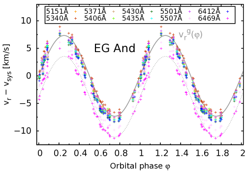
Figure 1: Orbital variability in RVs of individual Fe I absorption lines (the corresponding colours are given in the legend). The solid grey line represents the RV curve of the RG, $v_{r}^{\rm g}$, of Kenyon & Garcia (2016). Negative shifts of Fe I RV curves with respect to the $v_{r}^{\rm g}$ curve indicate an outflow of matter from the donor star. The Fe I 6469 Å  line shows the highest outflow velocities, with an average value of $-3.8$ km s^-1(dotted line). At $\varphi\approx 0$ - $0.2$, low inflow velocities are indicated for a fraction of Fe I lines. The data points are duplicated at orbital phases 1.0 - 2.0 for a more continuous view of the variability.

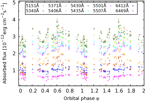
Figure 2: Orbital variability of the Fe I absorption lines fluxes. The strongest absorption near the superior conjunction of the RG suggests the highest Fe I column densities between the RG and the apex of the neutral wind cone-shaped region (Sect. 1 and 3.1). The data points are duplicated at orbital phases 1.0 - 2.0 for more continuous view of the variability.

The resulting variability in RV values, $v_{r}$, is plotted in Fig. 1 together with the RV curve of the RG according to the solution of Kenyon & Garcia (2016). Shifts up to $\approx-5$  km s^-1 in the RVs of individual Fe I absorption lines relative to the RG curve are measured. This is consistent with a slow outflow of the absorbing material. However, around orbital phases $\varphi\approx 0$ - $0.2$, the RV values especially of the Fe I 5340 Å line suggest a slow inflow.

The orbital variability of the fluxes (Fig. 2) shows the strongest absorption around the orbital phase $\approx 0.6,$ and the possible weakest absorption can be indicated at $\varphi\approx 0.1$, but there is a lack of the data around this orbital phase. When the conical shape of the neutral wind area around the RG is taken into account (Vogel 1991, also Sect. 1), this result points to the highest densities of the wind between the RG and the apex of the neutral area cone (Fig. 3). This agrees with the orbital variability of the absorption and the core-emission component of the H$\alpha$ line, which suggests that high-density matter lies in the area between the binary stellar components (Shagatova et al. 2021). The complete list of measured RV and flux values is given in Tables 3 and 4 in the appendix.

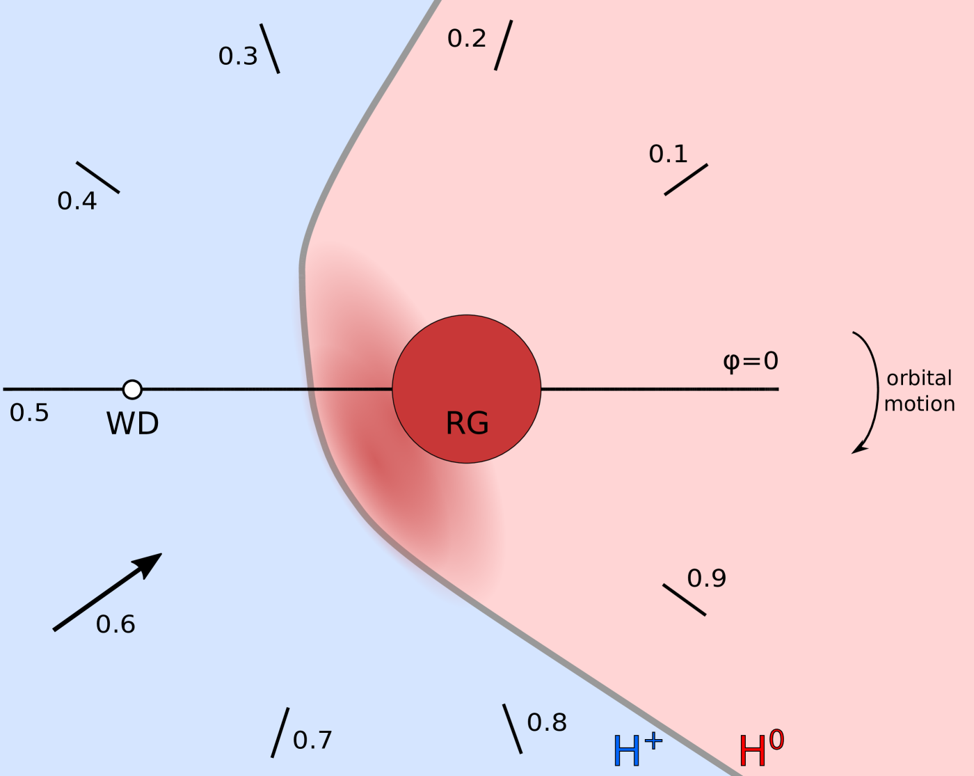
Figure 3: Sketch of the ionization structure of EG And at the orbital plane (adapted from Shagatova et al. 2021). The density enhancement in the neutral wind zone is indicated in the direction towards the white dwarf, with the maximum column density at orbital phase $\approx 0.6$, causing the highest absorption in the Fe I lines (Sec. 3.1).

3.2 Model atmosphere grid

The spread of RV values of the Fe I absorption lines within $\approx-5/+3$ km s^-1around the RV curve of the RG, $v_{r}^{\rm g}$ (Fig. 1) suggests that these lines originate in the vicinity of the stellar surface. To match the velocities with a depth in the RG atmosphere through modelling the profiles of Fe I lines (Sect. 3.3), we constructed a semi-empirical model atmosphere. This model is based on a simplified extension of the MARCS model atmosphere (Gustafsson et al. 2008) up to a distance of 150 $R_{\rm g}$ from the stellar centre. We defined the distribution of three physical parameters in the atmosphere as a logarithmically spaced grid: the neutral hydrogen density $N_{\rm H}$ [cm^-3], temperature $T$ [K], and electron pressure $P_{\rm e}$ [Ba] over the required range of radial distance $r$ [$R_{\rm g}$].

The MARCS model atmosphere extends up to a distance of 1.1 $R_{\rm g}$ from the stellar centre. From the available database, we selected the model with parameters closest to those of the RG in EG And (Sect. 1), a moderately CN-cycled model with ¹²C/¹³C$=20$, with a spherical geometry, effective temperature $T_{\rm eff}=3700$ K, mass $M=1.0$ $M_{\odot}$, $\log g=0.5$, metallicity [Fe/H] $=0,$ and microturbulence parameter of 2 km s^-1, which is a typical value for RGs in S-type SySts (Gałan et al. 2016, 2017). The selected model atmosphere corresponds to a star with a radius $R=93$ $R_{\odot}$  and a luminosity $L=1478$ $L_{\odot}$.

Beyond the radial distances covered by the MARCS atmosphere, we set the extrapolation up to $r=150$ $R_{\rm g}$, where the wind density is sufficiently low to have a negligible impact on the Fe I line absorption profile. At this outer edge of the atmosphere model, we estimated values of $N_{\rm H}$ and $T$ from the hydrodynamical simulation of the M-giant $\gamma$ Eri wind by Wood et al. (2016). We assessed the corresponding value of $P_{\rm e}$ for a representative value of the ionization fraction $\approx 10^{-6}$ for dense interstellar medium clouds (Williams et al. 1998; Caselli 2002; Bron et al. 2021).

We defined the values of the physical parameters $N_{\rm H}$, $T$ and $P_{\rm e}$ between a radial distance 1.1 and 150 $R_{\rm g}$ by interpolating the corresponding functions (Table 1). The selection of the $N_{\rm H}(r)$ interpolation function has a crucial effect on the Fe I absorption line profile. We used the form corresponding to the model of measured H⁰ column densities of EG And by Shagatova et al. (2016),

$$N_{\rm H}(r)=\displaystyle\frac{n_{1}}{2\lambda_{1}R_{\rm g}}\frac{1+\xi r^{1-K}}{r^{2}},$$ (2)

where $n_{1}$, $\xi$ and $K$ are the model parameters, and $\lambda_{1}=\pi/2$ is the Abel operator eigenvalue (Knill et al. 1993). Since the column density model is most reliable at distances of $r$ of several $R_{\rm g}$, we applied the condition on the interpolation function (2) that $N_{\rm H}(r=3\,R_{\rm g})=1.6\times 10^{10}$ cm^-3, that is, it equals the value of model J ($i=80^{\circ}$) from Shagatova et al. (2016). This approach led to smooth profiles of the atmosphere parameters over the required range of radial distances (Fig. 4).

Finally, we took the asymmetric conical shape of the neutral wind zone into account. For orbital phases when the line of sight crosses the boundary between neutral and ionized wind, we estimated its distance from the RG surface from Fig. 6 in Shagatova et al. (2021). We assumed that only the neutral wind contributes to the absorption in Fe I lines. Therefore, we limited the radial size of the model atmosphere to the H${}^{0}/$H⁺ area border at these orbital phases. At the rest of the orbital phases, the radial length of the neutral area was assumed to be 150 $R_{\rm g}$.

Table 1: Model atmosphere. More details can be found in Sect. 3.2.

$r\,[R_{\rm g}]$	$1$ - $1.1$	$1.1$ - $150$	$150$
$N_{\rm H}$	MARCS	interpolation by function from Shagatova et al. (2016) a	$10^{4}$ cm-3  (Wood et al. 2016)
$T$	MARCS	interpolation by exponential + linear function	$30\,$K  (Wood et al. 2016)
$P_{e}$	MARCS	interpolation by exponential function	$10^{-17}\,$dyne/cm2 (dense ISM clouds) b

Notes.
^a  with the condition that for $r=3\,R_{\rm g}$, $N_{\rm H}$ equals the value of model J from Shagatova et al. (2016)

^b  derived for a typical value of the ionization fraction of $10^{-6}$ (Williams et al. 1998; Caselli 2002; Bron et al. 2021)

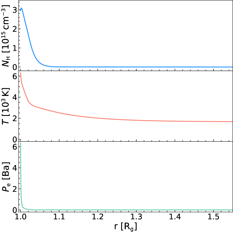
Figure 4: Distribution of the neutral hydrogen density $N_{\rm H}$, temperature $T,$ and electron pressure $P_{\rm e}$ in the semi-empirical model atmosphere defined for the range $1$ - $150$ $R_{\rm g}$ from the RG centre (Table 1 and Sect. 3.2).

3.3 Line profile of the Fe I absorption lines

To reproduce the spectral profiles of ten Fe I absorption lines from 5151 to 6469 Å at all orbital phases with a step of 0.1, we considered several broadening mechanisms that we incorporated into a custom Python code. We used the mass absorption coefficient including natural, pressure, thermal, and microturbulence broadening in the form given by Gray (2005). The values of the Ritz wavelengths, the inner quantum numbers J, the oscillator strengths, and the excitation potentials were acquired from the National Institute of Standards and Technology (NIST) database and the natural damping constants from the Vienna Atomic Line Database (VALD). The values of the partition functions for Fe I, Fe II, and Fe III were interpolated through the atmosphere grid from the tables of Halenka & Madej (2002) and Gray (2005). For the atmosphere layers with temperatures below 1000 K, we assumed constant partition functions. We calculated the values of the Hjerting function as the real part of the Fadeeva function with the wofz function within scipy.special library. The pressure broadening was treated as caused by the collisions with neutral hydrogen, using the impact approximation with line-broadening cross sections computed as a function of the effective principal quantum numbers (Anstee & O’Mara 1995; Barklem et al. 1998) with the tabulated values of the broadening cross-section $\sigma$ and velocity parameter $\alpha$ given by Barklem et al. (2000).

Furthermore, we included rotational broadening using the Python rotBroad function that is part of the PyAstronomy.pyasl library . Since the projected rotational velocity $v_{\rm rot}\sin(i)$ can be dependent on tidal forces in the outer regions of the RG (Mikołajewska et al. 2014), we allowed it to be a free parameter. After first fitting trials with a free linear limb-darkening coefficient $\varepsilon$, most of the fits converged to $\varepsilon=1$. As this is a reasonable value (tables of Neilson & Lester 2013), we kept $\varepsilon=1$ in all line-profile fits.

As the typical value of the macroturbulence velocity in RGs is $\approx 3$ km s^-1(Fekel et al. 2003), it adds to the broadening of the absorption-line profile. Often, the radial-tangential (RT) anisotropic macroturbulence is the preferred broadening model in a spectroscopic analysis (e.g. Carney et al. 2008; Simón-Díaz et al. 2017). On the other hand, Takeda & UeNo (2017) showed that the RT macroturbulence model is not adequate at least for solar-type stars because it overestimates turbulent velocity dispersion. They obtained more preferable results for the Gaussian anisotropic macroturbulence model. The resolution of our spectra and relatively low macroturbulent velocity does not allow us to distinguish between different macroturbulence models. Generally, there is agreement that neglecting macroturbulence as a source of line broadening leads to overestimated values of $v_{\rm rot}\sin(i)$, and, on the other hand, including a simple isotropic Gaussian macroturbulence model provides severely underestimated values of $v_{\rm rot}\sin(i)$ (Aerts et al. 2009; Simón-Díaz & Herrero 2014). Therefore, we decided to include the isotropic Gaussian model with two values of macroturbulence velocity, 0 and 3 km s^-1, to obtain lower and upper limits of $v_{\rm rot}\sin(i)$ values.

Finally, we included the instrumental broadening using a Gaussian kernel. The width of the Gaussian profile used in the convolution is given by the resolution $R$, which depends on the wavelength and was estimated using ThAr lines. For the wavelength range of the selected lines $5151-6469$ Å, the spectral resolution of our spectra ranges from $\approx 39100$ to $24000$. We used the broadGaussFast function from the PyAstronomy.pyasl library to include macroturbulent and instrumental broadening. The line profiles depicted at the right bottom panel of Fig. 5 compare the strength of individual broadening mechanisms.

We performed line profile modelling of Fe I lines at nine different orbital phases. Example fits at orbital phase $\varphi=0.1$ are depicted in Fig. 5. We evaluated the goodness of fit using the reduced $\chi$-square, $\chi_{\rm red}^{2}$. Its value is often $>2$ due to the low value of the degrees of freedom and the uncertain value of the standard observational error, which can vary from one observation to the next. We adopted a rather strict value of a $2\%$ standard deviation of the flux values for all observations to avoid overestimating the errors for the best-quality spectra. The errors due to the simplified model of macroturbulence are relatively small (Fig. 8 and 10) and have practically no effect on the resulting maximum depth of the origin of the spectral line in the atmosphere. The values of the $v_{\rm rot}\sin(i)$ parameter could be affected by unresolved blending of an absorption line.

An important source of systematic error can be introduced by the simplifications in our model, namely the symmetry of the wind distribution, which except for the shape of the neutral area, does not reflect the asymmetry of the egress/ingress and orbital-plane/pole-region in the distribution of the physical quantities (Fig. 4 of Dumm et al. (1999) and Fig. 8 of Shagatova et al. (2021)). Moreover, the particular shape of the neutral area itself represents a further source of systematic error. We estimated the distance from the RG centre to the ionization boundary by adapting the shape of the neutral area computed for the symbiotic binary SY Mus (Shagatova & Skopal 2017; Shagatova et al. 2021). This system comprises a white dwarf that is more luminous than the hot companion in EG And by two orders of magnitude (Muerset et al. 1991). On the other hand, the mass loss from its RG is probably higher (Muerset et al. 1991; Skopal 2005), leading to a denser wind zone. These characteristics affect the shape of the ionization boundary, and the actual shape for EG And can therefore deviate from the one in SY Mus. However, the similar measured egress values of the H⁰ column densities and the practically identical asymptote to the egress ionization boundary in the orbital plane, which is located at $\varphi\approx 0.17$ (Fig. 2b of Skopal 2023), strongly suggest that the ionization boundaries in these systems are similar. The lack of measured H⁰ column densities at ingress orbital phases for EG And precludes us from modelling the full shape of the ionization boundary. To estimate the sensitivity of the resulting physical parameters on the location of the ionization boundary, we performed fits for a shifted radial distance of the ionization boundary by $-0.5R_{\rm g}$ and $+0.5R_{\rm g}$ for a subset of modelled spectra with all Fe I absorption lines and orbital phases with the finite radial size of the neutral area represented. For the ionization boundary closer to the RG by $-0.5R_{\rm g}$, we obtained the same values of column densities or lower values by up to 6.0%, and for the boundary that is more distant by $+0.5R_{\rm g}$, the values were the same or higher by up to 1.1%. In both cases, higher values of the errors of $n_{\rm H}$ correspond to orbital phases $\approx$ 0.4 - 0.7, where the position of the ionization boundary is closer to the RG. The corresponding values of the projected rotational velocity $v_{\rm rot}\sin(i)$ remained unchanged for all fits, as did the values of the minimum distance from the RG centre $r$ (Sect. 3.4.1). This confirms the dominant role of the densest parts of the RG atmosphere in the formation of Fe I absorption line profiles. Given the rather low magnitude of the errors of $n_{\rm H}$ due to the uniform shifts and the most probably similar shape of the ionization structure for both systems, which is supported by similar profiles of the measured H⁰ column densities (Shagatova et al. 2016), an uncertain precise location of the apex of the neutral zone will probably not seriously affect the ratios of $n_{\rm H}$ values at individual orbital phases yielded by the line-profile modelling.

Another source of systematic error comes from the uncertain level of the continuum, which is mainly due to the spread in the photometric data. In our dataset, the typical deviation of the continuum values from the average relative to the flux ranges from 3% to 9% at the positions of individual Fe I absorption lines. This leads to errors in the $n_{\rm H}$ values with a magnitude of typically $\approx 10$ - $20$%, $v_{\rm rot}\sin(i)$ of $\approx 1$ - $7$% and a minimum distance $r$ of $\approx 0.1$ - $0.5$%. Therefore, the uncertainty in the level of the continuum represents a more significant source of error than the uncertainty in the position of the ionization boundary. Still, these systematic errors are of lower magnitude than the values of the standard deviations of the resulting values from the set of modelled spectra.

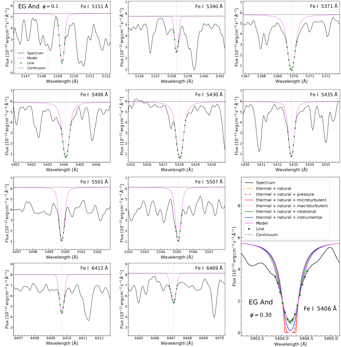
Figure 5: Example line-profile fits at orbital phase $\varphi=0.1$ with a macroturbulent velocity of 3 km s^-1. The bottom right panel shows a comparison of the strength of different broadening mechanisms in the line-profile model for the Fe I 5406 Å  line at $\varphi=0.3$.

3.4 Distribution of the physical parameters within the atmosphere

3.4.1 The height above the photosphere

Our models provided us with the total columns of the wind material that form the spectral profiles of individual Fe I lines in our set. From now on, the values of $r$ are understood as the distances of the lowest layers of the atmosphere model, corresponding to the resulting neutral columns from the line-profile fits. In other words, a particular value $r$ represents the maximum depth within the model atmosphere where the integration of the line-profile stops, and it corresponds to the deepest layer of the origin of the spectral line. The maximum depths of the Fe I line profile fits correspond to a relatively small height, $\approx 0.02$ to $\approx 0.06$ $R_{\rm g}$, above the RG photosphere. Figure 6 shows this result with the corresponding column densities. The resulting physical parameters averaged over the orbital phases are presented in Table 2. There is no sign of significant variations in the column density with orbital phase, but a slightly higher average value is measured at $\varphi=0.5-0.6$ (Fig. 7).

Table 2: Physical parameters $T$, $N_{\rm H}$, $n_{\rm H}$, $v_{r}$ , and $v_{\rm rot}\sin(i)$ averaged over $\varphi$ and their standard deviations, with the distance $r$ from the RG centre, corresponding to the lowest layer in the atmosphere of the total absorbing column for individual Fe I lines. The RV values averaged over all 53 observations (Sect. 2), $v^{\rm tot}_{r}$, are shown for comparison.

Fe I line	$r$	$T$	$N_{\rm H}$	$n_{\rm H}$	$v_{r}$	$v^{\rm tot}_{r}$	$v_{\rm rot}\sin(i)$
[Å]	[$R_{\rm g}$]	[K]	[1014cm-3]	[1025cm-2]	[ km s-1]
5151	1.021 $\pm$ 0.002	3599 $\pm$ 123	16.4 $\pm$ 2.0	13.6 $\pm$ 1.9	-0.37 $\pm$ 0.36	-0.29 $\pm$ 0.82	9.68 $\pm$ 1.05
5340	1.035 $\pm$ 0.008	3216 $\pm$ 198	7.7 $\pm$ 4.8	6.3 $\pm$ 3.9	0.59 $\pm$ 0.62	0.54 $\pm$ 0.83	12.17 $\pm$ 2.08
5371	1.036 $\pm$ 0.001	3149 $\pm$ 13	6.1 $\pm$ 0.4	4.9 $\pm$ 0.3	-0.42 $\pm$ 0.62	-0.38 $\pm$ 0.84	12.83 $\pm$ 0.99
5406	1.063 $\pm$ 0.001	2849 $\pm$ 11	0.8 $\pm$ 0.1	1.1 $\pm$ 0.1	-0.44 $\pm$ 0.55	-0.45 $\pm$ 0.90	11.15 $\pm$ 0.76
5430	1.032 $\pm$ 0.001	3212 $\pm$ 24	8.0 $\pm$ 0.7	6.4 $\pm$ 0.6	-0.95 $\pm$ 0.55	-0.82 $\pm$ 0.91	12.24 $\pm$ 0.47
5435	1.032 $\pm$ 0.002	3222 $\pm$ 30	8.3 $\pm$ 0.9	6.6 $\pm$ 0.7	-0.65 $\pm$ 0.44	-0.58 $\pm$ 0.92	10.49 $\pm$ 1.13
5501	1.018 $\pm$ 0.002	3823 $\pm$ 169	19.1 $\pm$ 1.8	16.6 $\pm$ 2.1	-0.22 $\pm$ 0.64	-0.10 $\pm$ 0.92	11.10 $\pm$ 1.00
5507	1.024 $\pm$ 0.003	3468 $\pm$ 125	14.1 $\pm$ 2.2	11.5 $\pm$ 2.1	-2.08 $\pm$ 0.57	-2.10 $\pm$ 0.90	10.78 $\pm$ 1.37
6412	1.045 $\pm$ 0.004	3034 $\pm$ 47	3.3 $\pm$ 1.0	2.9 $\pm$ 0.7	-0.74 $\pm$ 0.56	-0.82 $\pm$ 0.85	9.62 $\pm$ 2.12
6469	1.024 $\pm$ 0.002	3456 $\pm$ 92	14.0 $\pm$ 1.7	11.3 $\pm$ 1.6	-3.65 $\pm$ 0.87	-3.79 $\pm$ 0.87	8.48 $\pm$ 3.09

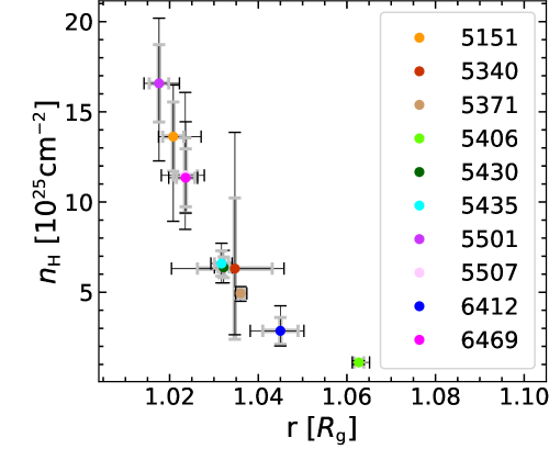
Figure 6: Column density as a function of the average minimal distance $r$ from the RG centre over our set of orbital phases and models with and without macroturbulence for individual Fe I absorption lines (dots), based on the values in Table 2. The grey error bars show the standard deviation, and the black error bars represent the total range of determined $r$ from the models.

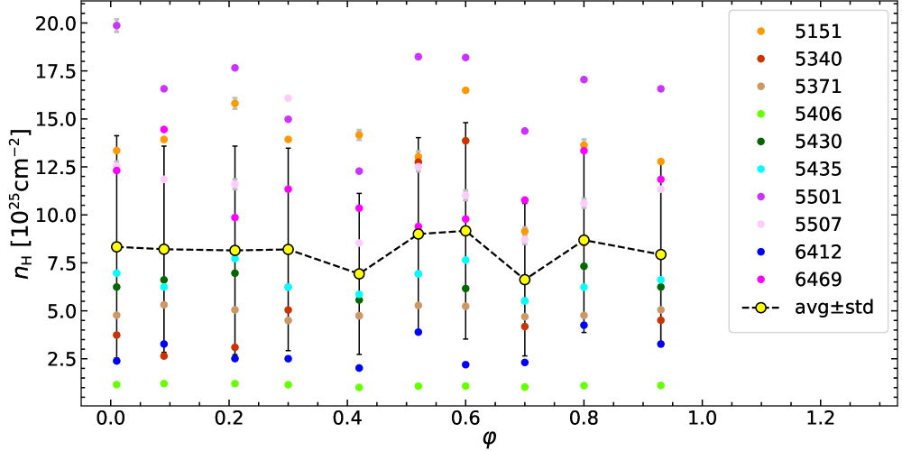
Figure 7: $n_{\rm H}$ values as a function of orbital phase for individual Fe I absorption lines and their averages. For most values, the differences between the models with and without macroturbulence are smaller than the size of the data points. When they are larger, they are shown as grey error bars.

3.4.2 Radial velocities

The total average and standard deviation over ten modelled spectra and ten Fe I absorption lines corresponds to RV $-0.89\pm 1.26$ km s^-1at a radial distance $1.03\pm 0.01$ $R_{\rm g}$ (Fig. 8). Assuming a terminal velocity of 30 km s^-1, we compared our RV values with velocity profiles obtained for EG And from modelling the measured column densities by Shagatova et al. (2016). As shown in Fig. 9, our results support very slow wind velocities close to the RG surface before the acceleration of the wind starts.

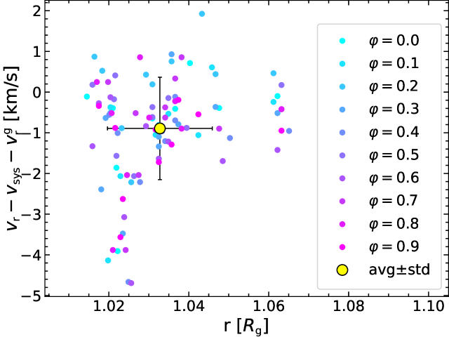
Figure 8: Distribution of RVs, corrected for the systematic velocity and orbital motion of the RG, along the radial direction at different orbital phases. The differences between models with and without macroturbulence are smaller than the size of data points. The large yellow circle corresponds to the average value of all RV values, and the black error bars show the standard deviation.

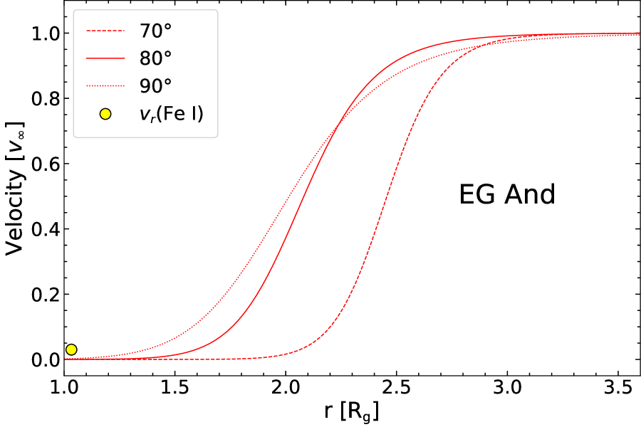
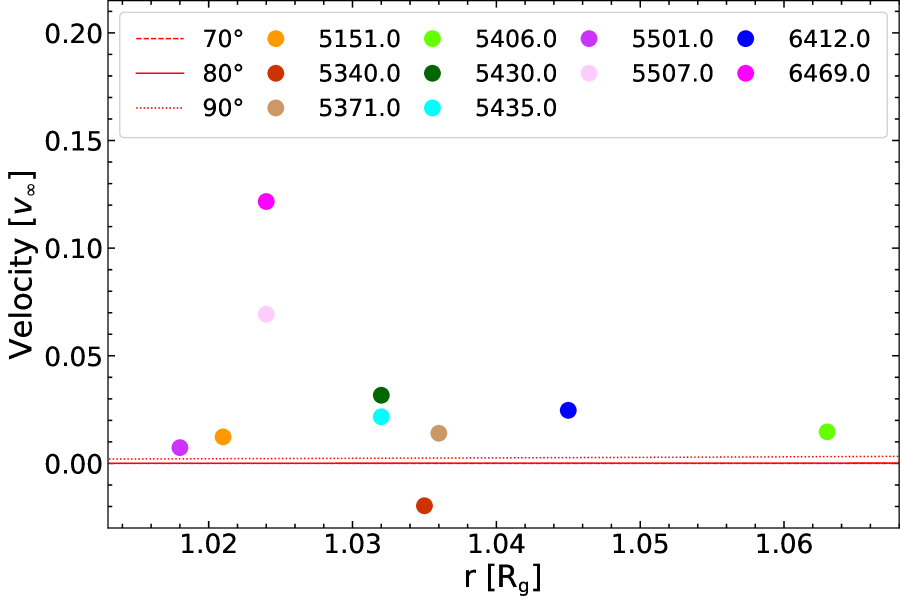
Figure 9: Comparison of the wind velocity profiles of RG in EG And (Shagatova et al. 2016) with the RV values of the Fe I absorption lines, $v_{r}(\rm Fe\,I)$, that were paired with the distance $r$ by the line-profile modelling (Sect. 3.3). In the top panel, the $v_{r}(\rm Fe\,I)$ data point represents the average value over all modelled spectra (Sect. 3.4.2). The bottom panel is a zoomed view with $v_{r}(\rm Fe\,I)$ values for the individual Fe I lines averaged over the orbital phases.

3.4.3 Rotational velocities

The orbit-averaged values of the projected rotational velocities of all modelled lines fall within 9.6 - 12.8 km s^-1  with standard deviations of 4 - 22% (Table 2), except for the Fe I 6469 Å  line with $v_{\rm rot}\sin(i)=8.5$ and a significantly higher standard deviation of 36%. While it is reasonable not to expect the same rotational velocity in any depth in the RG atmosphere, the measured differences can in part be caused by errors due to the blending of the lines. Moreover, the reliability of the $v_{\rm rot}\sin(i)$ determination is affected by the comparable strength of the instrumental broadening. The average and standard deviation over the whole sample of ten line-profile models per ten fitted lines corresponds to $v_{\rm rot}\sin(i)=10.9\pm 2.0$ km s^-1, which is in a typical range of $\approx 5$ - $11$ km s^-1determined for RGs in S-type SySts (Zamanov et al. 2008; Gałan et al. 2016, 2017). There are also much faster rotators in this group of stars with $v_{\rm rot}\sin(i)$ up to $\approx 50$ km s^-1 (Zamanov et al. 2007).

Assuming an orbital inclination of $i=80^{\circ}\pm 10^{\circ}$, we obtained $v_{\rm rot}=11.1_{-2.2}^{+2.6}$ km s^-1. Then, for RG radius $R_{\rm g}=75\pm 10$ $R_{\odot}$, the proportion of orbital to rotational period is $P_{\rm orb}/P_{\rm rot}=1.4_{-0.4}^{+0.6}$. Therefore, it is possible that the rotation of the RG is bounded to its orbital motion.

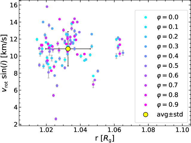
Figure 10: As in Fig. 8, but for projected rotational velocity. The grey error bars correspond to the difference between the models with and without macroturbulent broadening. Where no error bar is visible, the difference is smaller than the size of a data point.

4 Discussion

For our sample of ten Fe I absorption lines, we determined the absorbed flux and RV from their Gaussian fits (Sect. 3.1). Both quantities show the relative displacements for individual lines along the orbit (Figs. 1 and 2). The largest average shift in RVs by $-3.8$ km s^-1 with respect to the $v_{r}^{\rm g}(\varphi)$ curve is shown by the Fe I 6469 Å line (Fig. 1, dotted line). Around $\varphi=0.1$, the RVs of many lines indicate a slow flow of absorbing material towards the RG, especially the Fe I 5340 Å line with an average RV shift of $+0.5$ km s^-1.

The line-profile models accounting for several broadening mechanisms at the selected ten orbital phases (Sect. 3.3) enabled us to match their RV values with the deepest layer of the atmosphere, where the absorption line is predominantly created, characterized by $r$, $T$, $N_{\rm H}$ and $P_{\rm e}$ values. For the resulting depths in the range of $1.02$ - $1.06$  $R_{\rm g}$, all averaged RV values are low. Specifically, the outflow values lie within the interval from $-0.2$ to $-3.7$ km s^-1  (Table 2). This represents $0.7$ - $12.3\,\%$ of the estimated terminal wind velocity of $30$ km s^-1. While the typical RV at $r\approx 1.03$ $R_{\rm g}$ is $\approx 1$ km s^-1  ($\approx 3\%$ of $v_{\infty}$), there is a considerable dispersion in individual RV values (Fig. 9, bottom). The highest range of RV values is measured at the shortest distances of $\approx 1.02$ - $1.03$ $R_{\rm g}$. This variability can be a result of the highly complex flows of matter in the close surroundings of cool evolved stars (Kravchenko et al. 2018).

In the light of our results, the orbital phase $\approx 0.6$ seems to be exceptional in several ways. First, most of the Fe I lines from our set reach the maximum absorbed flux at this orbital phase (Fig. 2), pointing to a higher column density in the neutral zone between the apex of its cone and the RG, that is, in the direction towards the white dwarf companion (Fig. 3). In the same way, we could interpret the local maxima in the resulting column densities of the line-profile models (Fig. 7). Simultaneously, a higher dispersion of the RV values and the overall highest outflow velocities were measured around this orbital phase, suggesting enhanced outflow of the wind. The same feature was observed for the core-emission and absorption components of the H$\alpha$ line at orbital phases $0.6-0.7$ (Shagatova et al. 2021). Higher densities and, at the same time, higher velocities of the neutral matter may represent a challenge for hydrodynamical simulations of outflows from evolved cool stars in binary systems.

In our previous work, we investigated the geometrical distribution of the RG wind in EG And. By modelling H⁰ column densities, we found that the wind from the RG is focused towards the orbital plane (Shagatova et al. 2016). On the other hand, the RV orbital variability of the [OIII] 5007 Å  line, which coincides with the $v_{r}^{\rm g}(\varphi)$ curve in both phase and amplitude, indicates a dilution of the wind around the poles of the RG (Shagatova et al. 2021). However, the underlying mechanism that focuses wind in this system remains unclear. Skopal & Cariková (2015) applied the wind-compression disk model proposed by Bjorkman & Cassinelli (1993) to RGs in S-type symbiotic systems with rotational velocities of 6-10 km s^-1and found that the wind focusing occurs at the equatorial plane with a factor of 5–10 relative to the spherically symmetric wind. The average value $v_{\rm rot}=11.1$ km s^-1(Sect. 3.4.3) is therefore sufficiently high for rotation-induced compression of the wind from the giant in EG And.

The wind focusing can also potentially explain the higher densities of the neutral wind between the binary components, in contrast to the lower densities in the opposite direction, even though the neutral zone is more extended there. However, the wind compression by the RG rotation cannot explain this asymmetry because this mechanism acts equally strongly in all outward directions in the plane perpendicular to the rotational axis. Therefore, the gravitational effect of the white dwarf companion is the more natural explanation for this measured asymmetry. In a recent 3D hydrodynamical simulation of the accretion process for representative parameters of S-type symbiotic systems by Lee et al. (2022), the centre of the oblique region with highest densities around the RG is shifted towards the white dwarf, and the wind enhancement in the area of the orbital plane is also visible in their Fig. 2. For S-type system, recurrent nova RS Oph, the simulations of Booth et al. (2016) showed a dense equatorial outflow in the system as a result of the interaction of a slow wind with a binary companion. Therefore, gravitational focusing likely shapes the circumstellar matter in S-type SySts, as well as in D-type systems (de Val-Borro et al. 2009).

Often, the analysis of spectral lines in stellar atmospheres is focused on the determination of elemental abundances and basic stellar parameters by comparing synthetic and observational spectra (e.g. Steinmetz et al. 2020; Fukue et al. 2021) In our work, we aimed to assess the physical conditions at different heights in the RG atmosphere in interacting binary star from Fe I absorption line profiles. In principle, this approach can also be used for isolated non-dusty RG stars, which can potentially have different wind velocity profiles. The presence of the companion of a mass-loosing star affects the flow of matter in the wind region. Its gravitational pull can support the wind outflow from the RG, and we cannot exclude that in the case of single RGs, the low-velocity region is more extended and the velocities are lower. To form an idea about the proportions of gravitational force of the two stellar components in EG And, we compared the values of the gravitational force of the white dwarf and RG at several distances $r$ on the line joining the two stars. When we assume the separation between the two components of $4.5R_{\rm g}$ from the interval given by Vogel (1991), the magnitude of the white dwarf force at $r=1.02-1.06\,R_{\rm g}$, where the Fe I absorption lines are predominantly created, is small but not negligible. It is about $2$% of the value of the RG gravitational force. At $r=1.5R_{\rm g}$, where the acceleration of the wind starts (Fig. 9, top), this value is $\approx 7$%, and at $r=2R_{\rm g}$ in the acceleration region, it is $\approx 17$%. At the location at $\approx 3R_{\rm g}$, where the terminal velocity of the wind is reached, the gravitational forces from the two stars are already comparable. Close to the RG surface, where most of the absorption in Fe I lines occurs, the gravitational effect of the white dwarf is small, and we do not observe any tendency in the wind RVs as a function of orbital phase (Fig. 8), that is, at different distances of the near-surface regions from the white dwarf companion. Therefore, the RVs near the surface of the RG in EG And are probably comparable to those in isolated giants with similar evolutionary and physical characteristics. In the future, modelling of the Fe I absorption line-profiles for single late-type giants can be used to probe this assumption.

5 Conclusions

The RVs of the investigated Fe I absorption lines trace the orbital motion of the giant in the binary star EG And. They are displaced from the RV curve of the giant by 0.1 to 3.8 km s^-1 (i.e. up to 13% of the terminal wind velocity), which indicates a slow outflow of mass from the RG (Fig. 1). Modelling of their profiles showed that they are formed at maximum depths from $\approx 0.02$ to $\approx 0.06$ $R_{\rm g}$ above the photosphere. The typical value of the RV at these distances is around 1 km s^-1, which is consistent with the previously determined wind velocity profile from measured values of H⁰ column densities (Fig. 9). It is interesting to note that several Fe I lines, especially the 5340 Å line, showed a slow inflow of the absorbing matter towards the RG around orbital phase 0.1. Together with the dispersion of the RV values of several  km s^-1, this may be a sign that the nature of the near-surface mass flows in the RG atmosphere is complex (Fig. 1 and 9, bottom).

The orbital variations of the Fe I absorption line fluxes (Fig. 2) indicate that higher-density matter resides in the region between the binary components than in other directions from the RG at the near-orbital plane area. This asymmetry can be the result of gravitational interaction of the white dwarf with the RG wind, as was indicated by numerical simulations of gravitationally focused winds in interacting binaries. The measured rotational velocity of the RG, $\approx 11.1$ km s^-1, suggests an additional compression of the wind from the giant towards the orbital plane due to its rotation. Our results therefore support the contribution of both mechanisms to the observed RG wind enhancement and its asymmetry in the orbital plane of EG And.

The results of measuring the wind density asymmetry in the near-orbital plane region are consistent with our previous results on the wind focusing (Shagatova et al. 2016, 2021). Our direct observational finding shows a wind density enhancement between the binary components. This confirms the high efficiency of the wind mass transfer in SySts.

Appendix A Radial velocities and fluxes of selected Fe I absorption lines

Table 3: Radial velocities [ km s^-1] of ten Fe I absorption lines from our 53 spectra (Sect. 3.1).

HJD	dateobs	phase	5151 Å	5340 Å	5371 Å	5406 Å	5430 Å	5435 Å	5501 Å	5507 Å	6412 Å	6469 Å
2457743.439	2016/12/20.939	0.630	$-100.433$	$-99.564$	$-101.119$	$-101.663$	$-101.064$	$-101.393$	$-100.912$	$-103.576$	$-101.377$	$-104.652$
2457914.508	2017/06/10.008	0.985	$-96.228$	$-95.340$	$-96.295$	$-96.376$	$-96.856$	$-96.584$	$-96.032$	$-97.854$	$-96.561$	$-99.639$
2457924.512	2017/06/20.012	0.006	$-95.142$	$-94.152$	$-94.849$	$-94.929$	$-95.397$	$-95.054$	$-94.684$	$-96.723$	$-95.791$	$-99.181$
2457926.523	2017/06/22.023	0.010	$-94.878$	$-93.954$	$-94.739$	$-94.764$	$-95.240$	$-95.064$	$-94.618$	$-96.451$	$-94.627$	$-98.536$
2457941.517	2017/07/07.017	0.041	$-94.165$	$-93.265$	$-94.056$	$-94.323$	$-94.618$	$-94.376$	$-93.762$	$-95.860$	$-94.471$	$-97.280$
2457964.549	2017/07/30.049	0.089	$-91.599$	$-90.550$	$-91.390$	$-91.409$	$-91.908$	$-91.822$	$-91.277$	$-93.156$	$-91.831$	$-95.114$
2458073.421	2017/11/15.921	0.314	$-88.743$	$-87.923$	$-88.748$	$-88.816$	$-89.213$	$-89.003$	$-88.640$	$-90.385$	$-88.948$	$-91.631$
2458080.387	2017/11/22.887	0.329	$-87.896$	$-87.388$	$-88.135$	$-87.856$	$-88.371$	$-88.272$	$-87.843$	$-89.656$	$-88.341$	$-91.072$
2458370.558	2018/09/09.058	0.930	$-98.878$	$-98.129$	$-99.020$	$-99.098$	$-99.458$	$-99.183$	$-98.432$	$-100.505$	$-98.778$	$-101.742$
2458900.210	2020/02/20.710	0.028	$-92.395$	$-91.631$	$-92.466$	$-92.443$	$-92.727$	$-92.389$	$-92.065$	$-94.140$	$-92.928$	$-96.204$
2458911.235	2020/03/02.735	0.050	$-91.755$	$-90.389$	$-91.513$	$-91.820$	$-92.031$	$-91.805$	$-91.350$	$-93.324$	$-91.467$	$-95.412$
2458914.242	2020/03/05.742	0.057	$-91.628$	$-90.462$	$-91.990$	$-92.019$	$-92.125$	$-91.962$	$-91.330$	$-93.651$	$-91.889$	$-95.305$
2458918.238	2020/03/09.738	0.065	$-90.959$	$-89.675$	$-91.254$	$-91.163$	$-91.350$	$-91.065$	$-90.779$	$-92.998$	$-91.417$	$-94.821$
2458926.248	2020/03/17.748	0.082	$-89.581$	$-89.041$	$-89.447$	$-89.626$	$-89.739$	$-89.666$	$-89.026$	$-91.350$	$-90.113$	$-94.362$
2458927.243	2020/03/18.743	0.084	$-89.551$	$-88.608$	$-89.415$	$-89.406$	$-89.707$	$-89.519$	$-88.990$	$-91.125$	$-90.206$	$-92.423$
2458928.246	2020/03/19.746	0.086	$-89.386$	$-88.900$	$-89.468$	$-89.321$	$-89.757$	$-89.437$	$-88.908$	$-91.165$	$-89.852$	$-93.099$
2459029.542	2020/06/29.042	0.296	$-88.445$	$-87.144$	$-88.782$	$-88.692$	$-89.248$	$-88.873$	$-88.282$	$-90.424$	$-88.476$	$-91.352$
2459045.538	2020/07/15.038	0.329	$-88.550$	$-87.657$	$-88.557$	$-88.563$	$-89.015$	$-88.675$	$-88.035$	$-90.338$	$-88.990$	$-91.735$
2459062.461	2020/07/31.961	0.364	$-90.054$	$-89.489$	$-90.100$	$-90.086$	$-90.507$	$-90.298$	$-89.912$	$-91.618$	$-90.938$	$-93.832$
2459063.521	2020/08/02.021	0.366	$-90.318$	$-89.774$	$-90.125$	$-90.245$	$-90.703$	$-90.465$	$-90.134$	$-91.953$	$-90.898$	$-93.966$
2459067.485	2020/08/05.985	0.374	$-90.994$	$-90.127$	$-90.851$	$-90.924$	$-91.380$	$-91.123$	$-90.781$	$-92.638$	$-91.394$	$-94.456$
2459074.547	2020/08/13.047	0.389	$-91.182$	$-90.236$	$-91.284$	$-91.309$	$-91.668$	$-91.523$	$-90.957$	$-93.152$	$-91.586$	$-94.642$
2459075.506	2020/08/14.006	0.391	$-91.504$	$-90.107$	$-91.115$	$-91.353$	$-91.602$	$-91.484$	$-90.909$	$-93.114$	$-91.685$	$-94.551$
2459090.373	2020/08/28.873	0.422	$-92.059$	$-91.213$	$-92.117$	$-92.230$	$-92.654$	$-92.507$	$-92.079$	$-93.790$	$-92.448$	$-95.882$
2459096.486	2020/09/03.986	0.434	$-92.649$	$-91.666$	$-92.763$	$-92.833$	$-93.307$	$-93.048$	$-92.490$	$-94.670$	$-93.155$	$-96.547$
2459105.508	2020/09/13.008	0.453	$-94.196$	$-93.320$	$-94.239$	$-94.350$	$-94.713$	$-94.587$	$-94.156$	$-96.049$	$-94.893$	$-97.830$
2459106.415	2020/09/13.915	0.455	$-94.423$	$-93.498$	$-94.426$	$-94.542$	$-94.837$	$-94.600$	$-94.316$	$-96.309$	$-94.834$	$-97.926$
2459108.412	2020/09/15.912	0.459	$-94.494$	$-93.651$	$-94.636$	$-94.721$	$-95.202$	$-94.877$	$-94.421$	$-96.596$	$-95.248$	$-98.256$
2459146.332	2020/10/23.832	0.538	$-97.464$	$-96.620$	$-97.563$	$-97.738$	$-98.156$	$-98.225$	$-97.031$	$-99.331$	$-98.070$	$-100.916$
2459150.411	2020/10/27.911	0.546	$-97.961$	$-97.297$	$-98.105$	$-98.353$	$-98.795$	$-98.531$	$-98.069$	$-99.868$	$-98.542$	$-101.628$
2459154.382	2020/10/31.882	0.554	$-98.500$	$-97.675$	$-98.725$	$-98.757$	$-99.221$	$-98.934$	$-98.555$	$-100.491$	$-98.892$	$-101.796$
2459163.305	2020/11/09.805	0.573	$-98.651$	$-97.658$	$-98.984$	$-99.012$	$-99.384$	$-99.087$	$-98.533$	$-100.715$	$-99.207$	$-102.302$
2459178.245	2020/11/24.745	0.604	$-99.419$	$-99.425$	$-100.456$	$-100.640$	$-101.095$	$-100.134$	$-100.276$	$-102.256$	$-100.769$	$-103.658$
2459179.269	2020/11/25.769	0.606	$-100.342$	$-99.480$	$-100.674$	$-100.816$	$-101.178$	$-100.969$	$-100.388$	$-102.308$	$-100.884$	$-103.805$
2459180.388	2020/11/26.888	0.608	$-100.724$	$-99.464$	$-100.794$	$-100.879$	$-101.284$	$-101.057$	$-100.506$	$-102.408$	$-100.966$	$-104.141$
2459185.349	2020/12/01.849	0.618	$-100.652$	$-99.732$	$-100.953$	$-101.121$	$-101.525$	$-101.341$	$-100.807$	$-102.837$	$-101.409$	$-104.103$
2459195.337	2020/12/11.837	0.639	$-100.929$	$-100.124$	$-101.164$	$-101.140$	$-101.479$	$-100.981$	$-100.755$	$-102.940$	$-101.763$	$-104.611$
2459203.355	2020/12/19.855	0.656	$-100.965$	$-100.147$	$-101.205$	$-101.314$	$-101.615$	$-101.314$	$-100.902$	$-102.956$	$-101.655$	$-104.816$
2459216.304	2021/01/01.804	0.683	$-101.904$	$-101.111$	$-102.219$	$-102.373$	$-102.558$	$-102.135$	$-101.939$	$-103.997$	$-102.512$	$-105.272$
2459224.429	2021/01/09.929	0.699	$-101.699$	$-100.956$	$-101.948$	$-102.063$	$-102.544$	$-102.067$	$-101.204$	$-103.854$	$-102.800$	$-105.642$
2459226.207	2021/01/11.707	0.703	$-102.216$	$-101.277$	$-101.806$	$-102.247$	$-102.355$	$-102.072$	$-101.709$	$-103.819$	$-102.914$	$-105.904$
2459246.276	2021/01/31.776	0.745	$-102.520$	$-101.513$	$-102.721$	$-102.976$	$-103.239$	$-102.844$	$-102.397$	$-104.721$	$-103.191$	$-106.213$
2459268.234	2021/02/22.734	0.790	$-102.291$	$-101.572$	$-102.495$	$-102.589$	$-103.117$	$-102.864$	$-102.289$	$-104.314$	$-103.058$	$-105.798$
2459271.248	2021/02/25.748	0.796	$-102.117$	$-100.977$	$-101.985$	$-102.485$	$-102.588$	$-102.776$	$-101.596$	$-104.014$	$-102.634$	$-105.638$
2459275.244	2021/03/01.744	0.805	$-102.122$	$-101.517$	$-102.193$	$-102.081$	$-102.412$	$-102.431$	$-102.027$	$-103.985$	$-102.784$	$-105.378$
2459344.565	2021/05/10.065	0.948	$-97.870$	$-97.448$	$-97.671$	$-97.590$	$-97.891$	$-97.674$	$-97.574$	$-99.327$	$-98.696$	$-101.306$
2459388.500	2021/06/23.000	0.039	$-92.442$	$-91.838$	$-92.638$	$-92.516$	$-92.952$	$-92.502$	$-92.312$	$-94.170$	$-93.570$	$-95.654$
2459392.538	2021/06/27.038	0.048	$-91.992$	$-91.281$	$-92.048$	$-92.067$	$-92.401$	$-92.181$	$-91.726$	$-93.784$	$-92.841$	$-95.512$
2459620.262	2022/02/09.762	0.520	$-96.121$	$-95.234$	$-96.073$	$-95.639$	$-96.524$	$-96.050$	$-95.524$	$-97.111$	$-96.638$	$-98.029$
2459624.261	2022/02/13.761	0.528	$-96.217$	$-95.364$	$-96.307$	$-96.532$	$-96.819$	$-96.632$	$-96.098$	$-97.353$	$-96.783$	$-99.876$
2459650.236	2022/03/11.736	0.582	$-98.709$	$-98.505$	$-99.005$	$-99.228$	$-99.298$	$-99.403$	$-98.704$	$-99.937$	$-99.639$	$-102.261$
2459698.566	2022/04/29.066	0.682	$-101.800$	$-101.271$	$-101.634$	$-100.861$	$-102.399$	$-101.919$	$-101.503$	$-102.754$	$-102.129$	$-104.318$
2459952.259	2023/01/07.759	0.208	$-87.028$	$-85.973$	$-87.218$	$-87.113$	$-87.509$	$-87.136$	$-86.707$	$-88.798$	$-87.256$	$-89.911$

Notes.
HJD stands for the heliocentric Julian date, ’dateobs’ is the civil date [UT] in the standard format, yyyy/mm/dd.ddd, and ’phase’ is the corresponding orbital phase according to Eq. (1).

Table 4: Absorbed fluxes [$10^{-12}$$\rm\,erg\,cm^{-2}\,s^{-1}$] of ten Fe I absorption lines from our 53 spectra (Sect. 3.1).

HJD	dateobs	phase	5151 Å	5340 Å	5371 Å	5406 Å	5430 Å	5435 Å	5501 Å	5507 Å	6412 Å	6469 Å
2457743.439	2016/12/20.939	0.630	$2.136$	$1.834$	$3.512$	$3.036$	$3.672$	$3.032$	$3.079$	$3.191$	$1.238$	$0.650$
2457914.508	2017/06/10.008	0.985	$1.371$	$0.945$	$2.780$	$2.437$	$2.663$	$2.074$	$2.099$	$2.499$	$1.199$	$0.829$
2457924.512	2017/06/20.012	0.006	$1.280$	$0.847$	$2.656$	$2.275$	$2.494$	$1.965$	$1.974$	$2.228$	$1.068$	$0.753$
2457926.523	2017/06/22.023	0.010	$1.341$	$0.888$	$2.705$	$2.422$	$2.634$	$2.085$	$2.074$	$2.438$	$1.174$	$0.812$
2457941.517	2017/07/07.017	0.041	$1.476$	$0.863$	$2.881$	$2.627$	$2.844$	$2.176$	$2.150$	$2.508$	$1.109$	$0.761$
2457964.549	2017/07/30.049	0.089	$1.374$	$0.866$	$2.821$	$2.474$	$2.716$	$2.136$	$2.081$	$2.408$	$1.142$	$0.827$
2458073.421	2017/11/15.921	0.314	$1.686$	$1.079$	$3.340$	$2.919$	$3.268$	$2.474$	$2.314$	$2.790$	$1.348$	$0.926$
2458080.387	2017/11/22.887	0.329	$1.649$	$1.120$	$3.278$	$2.805$	$3.185$	$2.435$	$2.384$	$2.806$	$1.293$	$0.978$
2458370.558	2018/09/09.058	0.930	$1.441$	$0.954$	$2.979$	$2.548$	$2.839$	$2.224$	$2.115$	$2.531$	$1.211$	$0.720$
2458900.210	2020/02/20.710	0.028	$1.430$	$1.012$	$2.939$	$2.525$	$2.797$	$2.125$	$2.060$	$2.431$	$0.894$	$0.524$
2458911.235	2020/03/02.735	0.050	$1.330$	$0.856$	$2.668$	$2.310$	$2.638$	$2.013$	$1.861$	$2.148$	$0.957$	$0.610$
2458914.242	2020/03/05.742	0.057	$1.229$	$0.719$	$2.458$	$2.132$	$2.490$	$1.903$	$1.803$	$2.044$	$1.016$	$0.546$
2458918.238	2020/03/09.738	0.065	$1.207$	$0.788$	$2.510$	$2.116$	$2.441$	$1.795$	$1.800$	$2.040$	$0.861$	$0.482$
2458926.248	2020/03/17.748	0.082	$1.212$	$0.749$	$2.542$	$2.142$	$2.443$	$1.853$	$1.822$	$2.222$	$0.865$	$0.432$
2458927.243	2020/03/18.743	0.084	$1.180$	$0.762$	$2.469$	$2.119$	$2.396$	$1.819$	$1.810$	$2.078$	$0.881$	$0.559$
2458928.246	2020/03/19.746	0.086	$1.186$	$0.715$	$2.471$	$2.118$	$2.380$	$1.819$	$1.782$	$2.068$	$1.011$	$0.604$
2459029.542	2020/06/29.042	0.296	$1.571$	$1.065$	$3.035$	$2.599$	$2.901$	$2.249$	$2.069$	$2.438$	$1.024$	$0.672$
2459045.538	2020/07/15.038	0.329	$1.449$	$0.971$	$2.821$	$2.435$	$2.711$	$2.090$	$1.992$	$2.337$	$1.047$	$0.659$
2459062.461	2020/07/31.961	0.364	$1.385$	$0.950$	$2.669$	$2.358$	$2.665$	$2.018$	$1.905$	$2.378$	$1.009$	$0.576$
2459063.521	2020/08/02.021	0.366	$1.390$	$0.985$	$2.724$	$2.375$	$2.674$	$2.015$	$1.934$	$2.407$	$0.963$	$0.598$
2459067.485	2020/08/05.985	0.374	$1.375$	$0.970$	$2.744$	$2.396$	$2.681$	$2.032$	$1.977$	$2.364$	$0.926$	$0.643$
2459074.547	2020/08/13.047	0.389	$1.402$	$1.013$	$2.767$	$2.417$	$2.716$	$2.067$	$2.023$	$2.465$	$0.940$	$0.587$
2459075.506	2020/08/14.006	0.391	$1.556$	$0.977$	$2.798$	$2.423$	$2.675$	$2.065$	$2.014$	$2.389$	$0.925$	$0.568$
2459090.373	2020/08/28.873	0.422	$1.730$	$1.326$	$3.071$	$2.687$	$2.958$	$2.299$	$2.139$	$2.639$	$0.949$	$0.646$
2459096.486	2020/09/03.986	0.434	$1.735$	$1.377$	$3.180$	$2.792$	$3.113$	$2.404$	$2.276$	$2.784$	$0.767$	$0.408$
2459105.508	2020/09/13.008	0.453	$1.950$	$1.410$	$3.357$	$2.926$	$3.253$	$2.516$	$2.351$	$2.882$	$0.964$	$0.610$
2459106.415	2020/09/13.915	0.455	$1.962$	$1.424$	$3.452$	$2.934$	$3.260$	$2.515$	$2.374$	$2.797$	$0.945$	$0.655$
2459108.412	2020/09/15.912	0.459	$1.978$	$1.587$	$3.485$	$3.097$	$3.429$	$2.636$	$2.496$	$3.013$	$0.857$	$0.496$
2459146.332	2020/10/23.832	0.538	$1.785$	$1.319$	$3.067$	$2.682$	$3.096$	$2.369$	$2.139$	$2.696$	$1.080$	$0.669$
2459150.411	2020/10/27.911	0.546	$1.765$	$1.266$	$3.033$	$2.644$	$2.888$	$2.199$	$2.139$	$2.504$	$1.002$	$0.632$
2459154.382	2020/10/31.882	0.554	$1.805$	$1.382$	$3.120$	$2.749$	$2.968$	$2.370$	$2.257$	$2.658$	$1.074$	$0.641$
2459163.305	2020/11/09.805	0.573	$1.708$	$1.375$	$2.946$	$2.627$	$2.823$	$2.203$	$2.165$	$2.561$	$1.021$	$0.662$
2459178.245	2020/11/24.745	0.604	$2.721$	$1.733$	$3.909$	$3.285$	$3.589$	$3.067$	$2.615$	$3.095$	$1.069$	$0.627$
2459179.269	2020/11/25.769	0.606	$2.259$	$1.795$	$4.029$	$3.503$	$3.852$	$3.208$	$2.897$	$3.381$	$0.935$	$0.519$
2459180.388	2020/11/26.888	0.608	$2.213$	$1.739$	$3.930$	$3.380$	$3.630$	$2.835$	$2.624$	$3.156$	$1.047$	$0.663$
2459185.349	2020/12/01.849	0.618	$2.097$	$1.558$	$3.464$	$2.984$	$3.262$	$2.645$	$2.437$	$2.806$	$1.106$	$0.677$
2459195.337	2020/12/11.837	0.639	$1.803$	$1.354$	$3.197$	$2.796$	$3.038$	$2.406$	$2.257$	$2.685$	$1.064$	$0.699$
2459203.355	2020/12/19.855	0.656	$1.949$	$1.569$	$3.368$	$3.008$	$3.248$	$2.520$	$2.423$	$2.830$	$1.063$	$0.717$
2459216.304	2021/01/01.804	0.683	$1.963$	$1.348$	$3.518$	$2.964$	$3.250$	$2.561$	$2.471$	$2.794$	$1.031$	$0.680$
2459224.429	2021/01/09.929	0.699	$1.984$	$1.438$	$3.540$	$2.965$	$3.308$	$2.632$	$2.498$	$2.874$	$1.027$	$0.681$
2459226.207	2021/01/11.707	0.703	$1.935$	$1.309$	$3.436$	$2.930$	$3.160$	$2.478$	$2.424$	$2.710$	$1.137$	$0.700$
2459246.276	2021/01/31.776	0.745	$1.623$	$1.200$	$3.375$	$2.866$	$3.162$	$2.495$	$2.464$	$2.785$	$1.157$	$0.754$
2459268.234	2021/02/22.734	0.790	$1.591$	$1.076$	$3.169$	$2.747$	$3.035$	$2.398$	$2.241$	$2.628$	$1.052$	$0.748$
2459271.248	2021/02/25.748	0.796	$1.587$	$1.117$	$3.102$	$2.697$	$3.301$	$2.463$	$2.356$	$2.642$	$1.239$	$0.769$
2459275.244	2021/03/01.744	0.805	$1.564$	$1.083$	$3.140$	$2.719$	$3.076$	$2.430$	$2.300$	$2.738$	$1.206$	$0.709$
2459344.565	2021/05/10.065	0.948	$1.503$	$1.073$	$3.108$	$2.773$	$3.102$	$2.409$	$2.311$	$2.643$	$1.215$	$0.732$
2459388.500	2021/06/23.000	0.039	$1.467$	$1.018$	$3.077$	$2.692$	$3.006$	$2.394$	$2.250$	$2.603$	$1.373$	$0.756$
2459392.538	2021/06/27.038	0.048	$1.402$	$0.903$	$2.962$	$2.581$	$2.856$	$2.258$	$2.168$	$2.595$	$1.420$	$0.797$
2459620.262	2022/02/09.762	0.520	$1.326$	$1.119$	$2.983$	$2.423$	$2.880$	$2.184$	$2.140$	$2.156$	$1.058$	$0.502$
2459624.261	2022/02/13.761	0.528	$1.375$	$1.076$	$2.876$	$2.472$	$2.837$	$2.192$	$2.172$	$2.142$	$1.123$	$0.615$
2459650.236	2022/03/11.736	0.582	$1.450$	$1.035$	$2.891$	$2.578$	$2.995$	$2.340$	$2.311$	$2.199$	$1.029$	$0.609$
2459698.566	2022/04/29.066	0.682	$1.248$	$0.871$	$2.717$	$2.562$	$2.617$	$1.994$	$1.931$	$1.981$	$1.343$	$0.747$
2459952.259	2023/01/07.759	0.208	$1.698$	$1.349$	$3.490$	$3.083$	$3.458$	$2.702$	$2.552$	$3.058$	$1.073$	$0.880$