Constraints on primordial curvature power spectrum with pulsar timing arrays

Abstract

The stochastic signal detected by NANOGrav, PPTA, EPTA, and CPTA can be explained by the scalar-induced gravitational waves. In order to determine the scalar-induced gravitational waves model that best fits the stochastic signal, we employ both single- and double-peak parameterizations for the power spectrum of the primordial curvature perturbations, where the single-peak scenarios include the $\delta$-function, box, lognormal, and broken power law model, and the double-peak scenario is described by the double lognormal form. Using Bayesian inference, we find that there is no significant evidence for or against the single-peak scenario over the double-peak model, with $\log$ (Bayes factors) among these models $\ln\mathcal{B}<1$. Therefore, we cannot distinguish the different shapes of the power spectrum of the primordial curvature perturbation with the current sensitivity of pulsar timing arrays.

1 Introduction

Recently, four pulsar timing array (PTA) collaborations, namely NANOGrav [1, 2], PPTA [3, 4], EPTA [5, 6], and CPTA [7], all announced the strong evidence of a stochastic signal consistent the Hellings-Downs angular correlations, pointing to the gravitational-waves (GW) origin of this signal. Assuming the signal originates from an ensemble of binary supermassive black hole inspirals and a fiducial $f^{-2/3}$ characteristic-strain spectrum, the strain amplitude is estimated to be at the order of $\sim 10^{-15}$ at a reference frequency of $1\,\rm{yr}^{-1}$ [2, 4, 6, 7]. However, the origin of this signal, whether from supermassive black hole binaries or other cosmological sources, is still under investigation [8, 9, 10, 11, 12, 13, 14, 15, 16, 17, 18, 19, 20, 21, 22, 23, 24, 25, 26, 27, 28]. A promising candidate to explain the signal is the scalar-induced gravitational waves (SIGWs) accompanying the formation of primordial black holes [29, 30, 31, 32, 33, 34, 35, 36, 37, 38, 39, 40, 41, 42, 43, 44, 45, 46, 47]. Other physical phenomena (see e.g. [48, 49, 50, 51, 52, 53, 54, 55, 56, 57, 58, 59]) can also be the sources in the PTA band.

The SIGW is sourced from scalar perturbations generated during the inflationary epoch [60, 61, 62, 63, 64, 65, 66, 67, 68, 69, 70, 71, 72, 73, 74, 75, 76, 77, 78, 79, 80, 81, 82, 83]. They offer valuable insights into the physics of the early Universe and can be detected not only by PTAs but also by space-based GW detectors such as LISA [84, 85], Taiji [86], TianQin [87, 88], and DECIGO [89]. Significant SIGWs require the amplitude of the power spectrum of the primordial curvature perturbations to be around $\mathcal{A}_{\zeta}\sim\mathcal{O}(0.01)$ which is approximately seven orders of magnitude larger than the constraints from large-scale measurements of cosmic microwave background (CMB) anisotropy observation, $\mathcal{A}_{\zeta}=2.1\times 10^{-9}$ [90]. Therefore, to account for the observed gravitational wave signal detected by PTAs, the curvature power spectrum must possess at least one high peak. This can be achieved through inflation models with a transition ultra-slow-roll phase [91, 92, 93, 94, 95, 96, 97, 98, 99, 100, 101, 102, 103, 104, 105, 106, 107, 108, 109, 110, 111, 112, 113, 114, 115, 116, 117, 118, 119, 120, 121, 122, 123, 124, 125, 126, 127].

To characterize a single-peak primordial curvature power spectrum, various parameterizations such as the $\delta$-function form, box form, lognormal form, or broken power law form are employed. Among them, the $\delta$-function, box and lognormal parameterizations are investigated in Ref. [8], where the constraints from the PTAs data on the parameters of these models are also given. The constraints on the broken power law form are provided in Ref. [10], where the role of non-Gaussianity is also considered. However, the analysis does not determine which model among these is the most compatible with the PTA signal. For the multi-peak primordial curvature power spectrum model [121], we parameterize the primordial curvature power spectrum with the double lognormal form. In this study, we aim to determine whether the PTA signal favors a single-peak or multi-peak primordial curvature power spectrum and identify the most compatible model with the PTA signal.

The organization of this paper is as follows: section 2 provides a brief review of the scalar-induced gravitational waves. Section 3 presents the constraints on the power spectrum for different forms and identifies the best-fitted model based on the PTAs signal. Finally, section 4 summarizes our findings and provides concluding remarks.

2 Scalar-induced gravitational waves

The large scalar perturbations seeded from the primordial curvature perturbation generated during inflation can act as the source to induce GWs at the radiation domination epoch where the equation of state is $w=1/3$. In this section, we give a brief review of the SIGW. In the cosmological background, the metric with perturbation in Newtonian gauge is [128]

$$ds^{2}=-a^{2}(\eta)(1+2\Phi)d\eta^{2}+a^{2}(\eta)\left[(1-2\Phi)\delta_{ij}+\frac{1}{2}h_{ij}\right]dx^{i}dx^{j},$$ (2.1)

where $a$ is the scale factor of the Universe, $\eta$ is the conformal time, $d\eta=dt/a(t)$, $\Phi$ is the Bardeen potential, and $h_{ij}$ are the tensor perturbations. The tensor perturbations in the Fourier space can be obtained by the transform

$$h_{ij}(\bm{x},\eta)=\int\frac{d^{3}ke^{i\bm{k}\cdot\bm{x}}}{(2\pi)^{3/2}}[h_{\bm{k}}(\eta)e_{ij}(\bm{k})+\tilde{h}_{\bm{k}}(\eta)\tilde{e}_{ij}(\bm{k})],$$ (2.2)

where the plus and cross polarization tensors $e_{ij}(\bm{k})$ and $\tilde{e}_{ij}(\bm{k})$ are

$$e_{ij}(\bm{k})=\frac{1}{\sqrt{2}}\left[e_{i}(\bm{k})e_{j}(\bm{k})-\tilde{e}_{i}(\bm{k})\tilde{e}_{j}(\bm{k})\right],$$ (2.3)

$$\tilde{e}_{ij}(\bm{k})=\frac{1}{\sqrt{2}}\left[e_{i}(\bm{k})\tilde{e}_{j}(\bm{k})+\tilde{e}_{i}(\bm{k})e_{j}(\bm{k})\right],$$ (2.4)

and the basis vectors satisfying $\bm{e}\cdot\tilde{\bm{e}}=\bm{e}\cdot\bm{k}=\tilde{\bm{e}}\cdot\bm{k}$.

With the source from the second order of linear scalar perturbations, the tensor perturbations with either polarization in the Fourier space satisfy [67, 68]

$$h^{\prime\prime}_{\bm{k}}+2\mathcal{H}h^{\prime}_{\bm{k}}+k^{2}h_{\bm{k}}=4S_{\bm{k}},$$ (2.5)

where $\mathcal{H}=a^{\prime}/a$ is the conformal Hubble parameter and a prime denotes the derivative with respect to the conformal time $\eta$. The second order source $S_{\bm{k}}$ is [67, 68, 71]

$$S_{\bm{k}}=\int\frac{d^{3}\tilde{k}}{(2\pi)^{3/2}}e_{ij}(\bm{k})\tilde{k}^{i}\tilde{k}^{j}\left[2\Phi_{\tilde{\bm{k}}}\Phi_{\bm{k}-\tilde{\bm{k}}}\phantom{\frac{1}{2}}+\frac{1}{\mathcal{H}^{2}}\left(\Phi^{\prime}_{\tilde{\bm{k}}}+\mathcal{H}\Phi_{\tilde{\bm{k}}}\right)\left(\Phi^{\prime}_{\bm{k}-\tilde{\bm{k}}}+\mathcal{H}\Phi_{\bm{k}-\tilde{\bm{k}}}\right)\right].$$ (2.6)

The Bardeen potential in the Fourier space, $\Phi_{\bm{k}}$, can be connected to the primordial curvature perturbations $\zeta_{\bm{k}}$ produced during inflation epoch through the transfer function,

$$\Phi_{\bm{k}}=\frac{2}{3}T(k\eta)\zeta_{\bm{k}},$$ (2.7)

and the transfer function $T(k\eta)$ satisfy

$$T(k\eta)=3\left[\frac{\sin\left({k\eta}/{\sqrt{3}}\right)-\left({k\eta}/{\sqrt{3}}\right)\cos\left({k\eta}/{\sqrt{3}}\right)}{\left({k\eta}/{\sqrt{3}}\right)^{3}}\right].$$ (2.8)

The equation of the tensor perturbations (2.5) can be solved by the Green’s function method and the solution is

$$h_{k}(\eta)=\frac{4}{a(\eta)}\int_{\eta_{k}}^{\eta}d\tilde{\eta}g_{k}(\eta,\tilde{\eta})a(\tilde{\eta})S_{k}(\tilde{\eta}),$$ (2.9)

where $g_{k}$ is the corresponding Green’s function satisfying the equation

$$g_{k}^{\prime\prime}(\eta,\tilde{\eta})+\left(k^{2}-\frac{a^{\prime\prime}}{a}\right)g_{k}(\eta,\tilde{\eta})=\delta(\eta-\tilde{\eta}).$$ (2.10)

During the radiation domination, the scale factor satisfies $a\propto\eta$ and $a^{\prime\prime}/a=0$, the Green’s function is

$$g_{k}(\eta,\tilde{\eta})=\frac{\sin\left[k(\eta-\tilde{\eta})\right]}{k}.$$ (2.11)

The definition of the power spectrum of tensor perturbations $h_{k}$ is

$$\langle h_{\bm{k}}(\eta)h_{\tilde{\bm{k}}}(\eta)\rangle=\frac{2\pi^{2}}{k^{3}}\delta^{(3)}(\bm{k}+\tilde{\bm{k}})\mathcal{P}_{h}(k,\eta).$$ (2.12)

Combining it with the solution of $h_{k}$, equation (2.9), we have [68, 67, 71, 129, 130]

$$\begin{split}\mathcal{P}_{h}(k,\eta)=&4\int_{0}^{\infty}dv\int_{|1-v|}^{1+v}du\left[\frac{4v^{2}-(1-u^{2}+v^{2})^{2}}{4uv}\right]^{2}\\ &\times I_{RD}^{2}(u,v,x)\mathcal{P}_{\zeta}(kv)\mathcal{P}_{\zeta}(ku),\end{split}$$ (2.13)

where $u=|\bm{k}-\tilde{\bm{k}}|/k$, $v=\tilde{k}/k$, $x=k\eta$, and $\mathcal{P}_{\zeta}$ is the power spectrum of the curvature perturbation which is parameterized in the following section. The integral kernel $I_{\text{RD}}$ is [71]

$$I_{\text{RD}}(u,v,x)=\int_{0}^{x}d\bar{x}\frac{\bar{x}}{x}\sin(x-\bar{x})f(v,u,\bar{x})$$ (2.14)

where

$$f(v,u,x)=\frac{4}{3}T(vx)T(ux)+\frac{4}{9}x\partial_{x}[T(vx)T(ux)]+\frac{4}{9}x^{2}\partial_{x}T(vx)\partial_{x}T(ux).$$ (2.15)

The definition of the energy density of gravitational waves is

$$\Omega_{\mathrm{GW}}(k,\eta)=\frac{1}{24}\left(\frac{k}{aH}\right)^{2}\overline{\mathcal{P}_{h}(k,\eta)}.$$ (2.16)

By combining the equation (2.13) and the definition (2.16), we obtain [129, 130]

$$\begin{split}\Omega_{\mathrm{GW}}(k,\eta)=&\frac{1}{6}\left(\frac{k}{aH}\right)^{2}\int_{0}^{\infty}dv\int_{|1-v|}^{1+v}du\times\left[\frac{4v^{2}-(1-u^{2}+v^{2})^{2}}{4uv}\right]^{2}\\ &\times\overline{I_{\text{RD}}^{2}(u,v,x)}\mathcal{P}_{\zeta}(kv)\mathcal{P}_{\zeta}(ku),\end{split}$$ (2.17)

where $\overline{I_{\text{RD}}^{2}}$ represents the oscillation time average of the integral kernel. After the horizon reentry and the scale is well within the horizon, $k/aH\gg 1$ and $x\gg 1$, the oscillate average $\overline{I_{\text{RD}}^{2}}$ can expressed as [71]

$$\overline{I_{\text{RD}}^{2}(v,u,x\gg 1)}= \frac{1}{2x^{2}}\left[\frac{3(u^{2}+v^{2}-3)}{4u^{3}v^{3}}\right]^{2}\bigg{[}\left(-4uv+(u^{2}+v^{2}-3)\log\left|\frac{3-(u+v)^{2}}{3-(u-v)^{2}}\right|\right)^{2}$$

$$\qquad\qquad\qquad+\pi^{2}(u^{2}+v^{2}-3)^{2}\Theta(v+u-\sqrt{3})\bigg{]}.$$ (2.18)

In the radiation-dominated era, $k/aH=x$, the term $(k/aH)^{2}$ in the front of equation (2.17) can be balanced by the $1/x^{2}$ term in the front of equation (2), implying that the GW energy density expression in equation (2.17) becomes independent on the conformal time and only dependent on the scale $k$.

After generation, the energy density of gravitational waves evolves in the same way as radiation. Using this property, it is straightforward to determine the energy density of gravitational waves at present. The relation of the GW energy density at present and the generation is [131]

$$\Omega_{\text{GW}}(k,\eta_{0})=\left[\frac{a^{2}(\eta)H(\eta)}{a^{2}_{0}H_{0}}\right]^{2}\Omega_{\text{GW}}(k,\eta),$$ (2.19)

where the subscript “0” denotes the value at present. Assuming the entropy of the Universe is conserved, we can obtain [109]

$$H^{2}(\eta)=a^{-4}(\eta)\left(\frac{g_{*,s}^{4}g_{*}^{-3}}{g_{*,s0}^{4}g_{*,0}^{-3}}\right)^{-1/3}H_{0}^{2}\Omega_{r,0},$$ (2.20)

where $\Omega_{r,0}$ is the current energy density of the radiation, $g_{*}$ is the number of relativistic degrees of freedom, $g_{*,s}$ is the number of entropy degrees of freedom, $g_{*,0}=3.36$, $g_{*,s0}=3.91$, and $a_{0}=1$. Substituting equation (2.20) into equation (2.19), we obtain the energy density of the SIGWs at present

$$\Omega_{\mathrm{GW}}(k,\eta_{0})=c_{g}\Omega_{r,0}\Omega_{\mathrm{GW}}(k,\eta),$$ (2.21)

where [132, 133]

$$c_{g}=0.387\left(\frac{g_{*,s}^{4}g_{*}^{-3}}{106.75}\right)^{-1/3}.$$ (2.22)

3 Models and results

At large scales, the observational data from the CMB impose a constraint on the amplitude of the primordial curvature power spectrum, which is limited to $\mathcal{A}_{\zeta}=2.1\times 10^{-9}$ [90]. However, there are minimal constraints on the primordial curvature power spectrum at small scales. Consequently, in order to generate significant SIGWs, it is necessary to enhance the primordial curvature power spectrum to approximately $\mathcal{A}_{\zeta}\sim\mathcal{O}(0.01)$ at small scales. Thus, the profile of the primordial curvature spectrum exhibits at least one pronounced peak at intermediate scales, while displaying lower amplitudes at both large and very small scales. In this section, we consider the primordial curvature spectrum with single-peak and double-peak, respectively. For the single peak, the commonly employed parameterizations of the primordial curvature spectrum are the simple $\delta$ function form

$$\mathcal{P}_{\zeta}=A\delta(\ln k-\ln k_{p}),$$ (3.1)

the box form

$$\mathcal{P}_{\zeta}=A\Theta(k-k_{\mathrm{min}})\,\Theta(k_{\mathrm{max}}-k),$$ (3.2)

the lognormal form

$$\mathcal{P}_{\zeta}=\frac{A}{\sqrt{2\pi}\Delta}\exp\left[-\frac{1}{2}\left(\frac{\ln k-\ln k_{p}}{\Delta}\right)^{2}\right],$$ (3.3)

and the broken power law form

$$\mathcal{P}_{\zeta}=\frac{A(\alpha+\beta)}{\beta(k/k_{p})^{-\alpha}+\alpha(k/k_{p})^{\beta}}+A_{*}(k/k_{*})^{n_{s_{*}}-1},$$ (3.4)

with $n_{s_{*}}=0.965$, $k_{*}=0.05\mathrm{Mpc}^{-1}$, and $A_{*}=2.1\times 10^{-9}$ [134]. For the double peak model, we parameterize the primordial curvature spectrum with a double lognormal form

$$\mathcal{P}_{\zeta}=\frac{A_{1}}{\sqrt{2\pi}\Delta_{1}}\exp\left[-\frac{1}{2}\left(\frac{\ln k-\ln k_{p_{1}}}{\Delta_{1}}\right)^{2}\right]+\frac{A_{2}}{\sqrt{2\pi}\Delta_{2}}\exp\left[-\frac{1}{2}\left(\frac{\ln k-\ln k_{p_{2}}}{\Delta_{2}}\right)^{2}\right].$$ (3.5)

We conducted a Bayesian analysis of the NANOGrav 15 yrs data to investigate the parameterization of the power spectrum of the primordial curvature perturbation, as described by Eqs. (3.1-3.5). In our analysis, we utilized the 14 frequency bins reported in [2, 8] to fit the posterior distributions of the model parameters. The Bilby code [135] was employed for the analysis, utilizing the dynesty algorithm for nested sampling [136]. The log-likelihood function was constructed by evaluating the energy density of SIGWs at the 14 specific frequency bins. Subsequently, we computed the sum of the logarithm of the probability density functions obtained from 14 independent kernel density estimates corresponding to these frequency values [137, 138, 139]. The equation for the likelihood function is presented as

$$\mathcal{L}(\mathbf{\Theta})=\prod_{i=1}^{14}\mathcal{L}_{i}\left(\Omega_{\mathrm{GW}}\left(f_{i},\mathbf{\Theta}\right)\right),$$ (3.6)

where $\bm{\Theta}$ is the collection of parameters for $\delta$-function, box, lognormal, broken power law, and double lognormal models. These parameters and their priors are shown in Table 1.

Model	Parameters	Prior	Posterior	${\rm{ln}}\mathcal{B}$
	${\rm{log_{10}}}\,A$	$U[-3,4]$	$1.28^{+1.79}_{-1.95}$
$\delta$-function	${\rm log_{10}}\,k_{p}\,/\,{\rm Mpc^{-1}}$	$U[5,14]$	$11.19^{+1.99}_{-2.26}$	$0.29$
	${\rm log_{10}}\,A$	$U[-3,1]$	$-0.95^{+0.52}_{-0.28}$
Box	${\rm log_{10}}\,k_{\mathrm{min}}\,/\,{\rm Mpc^{-1}}$	$U[5,10]$	$7.40^{+0.47}_{-0.31}$	$0.26$
	${\rm log_{10}}\,k_{\mathrm{max}}\,/\,{\rm Mpc^{-1}}$	$U[5,20]$	$13.77^{+4.24}_{-4.11}$
	${\rm log_{10}}\,A$	$U[-3,1]$	$-0.88^{+0.81}_{-0.36}$
	$\alpha$	$U[0,5]$	$2.33^{+1.72}_{-1.14}$
Broken power law	$\beta$	$U[0,5]$	$2.22^{+1.87}_{-1.53}$	$0.46$
	${\rm log_{10}}\,k_{p}\,/\,{\rm Mpc^{-1}}$	$U[5,10]$	$7.91^{+0.88}_{-0.44}$
	${\rm{log_{10}}}\,A$	$U[-3,1]$	$-0.26^{+0.60}_{-0.58}$
Lognormal	$\Delta$	$U[0,3]$	$1.66^{+0.65}_{-0.87}$	$0.45$
	${\rm log_{10}}\,k_{p}\,/\,{\rm Mpc^{-1}}$	$U[5,10]$	$8.61^{+0.93}_{-0.79}$
	${\rm{log_{10}}}\,A_{1}$	$U[-3,1]$	$-0.34^{+0.64}_{-0.61}$
	$\Delta_{1}$	$U[0,3]$	$1.32^{+0.77}_{-0.77}$
Double lognormal	${\rm log_{10}}\,k_{p_{1}}\,/\,{\rm Mpc^{-1}}$	$U[5,10]$	$8.21^{+0.92}_{-0.66}$	$0$
	${\rm{log_{10}}}\,A_{2}$	$U[-3,1]$	$-0.84^{+1.25}_{-1.49}$
	$\Delta_{2}$	$U[0,3]$	$1.67^{+0.94}_{-1.09}$
	${\rm log_{10}}\,k_{p_{2}}\,/\,{\rm Mpc^{-1}}$	$U[5,20]$	$14.40^{+3.75}_{-3.90}$

Table 1: The priors, maximum posterior values, 1-$\sigma$ credible intervals bounds of posteriors and Bayes factor for $\delta$-function, box, lognormal, broken power law, and double lognormal model of the primordial curvature power spectrum using NANOGrav 15-yr data set. Here, we set the double lognormal model as the fiducial model.

We divide these models into two categories. The first one is single-peak power spectrum models, including $\delta$-function (3.1), box (3.2), lognormal (3.3) and broken power law model (3.4), while the second one is double-peak model, including double lognormal model (3.5). The posterior distributions for the parameters in Eqs. (3.1-3.5) are depicted in Figures 1-5, respectively. We summarize the mean values and 1-$\sigma$ confidence intervals for parameters of these models in Table 1.

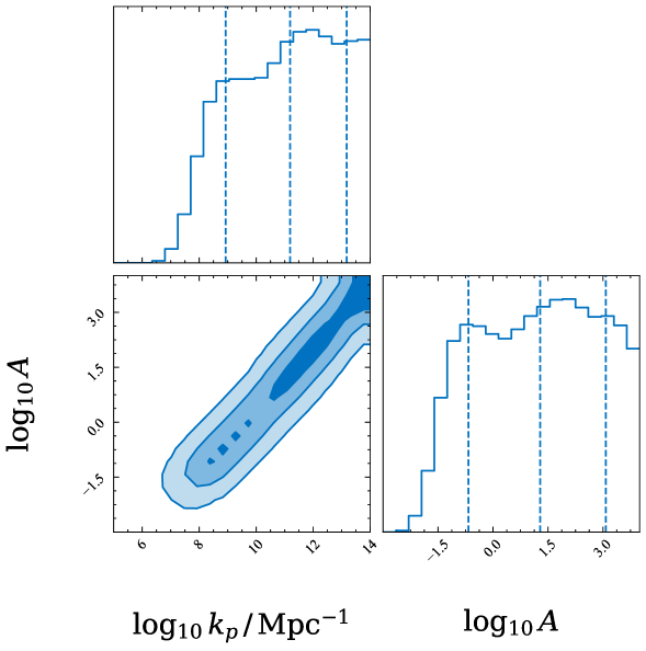
Figure 1: The posteriors of the parameters for the $\delta$-function parameterization (3.1).

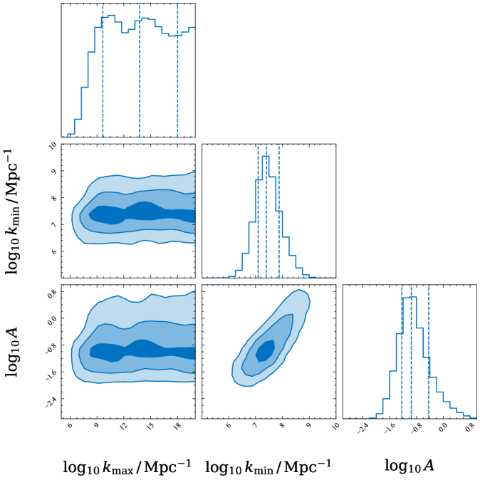
Figure 2: The posteriors of the parameters for the box parameterization (3.2).

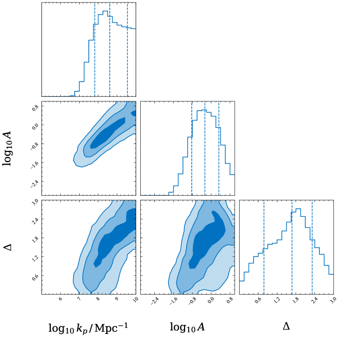
Figure 3: The posteriors on the parameters of the lognormal parameterization (3.3).

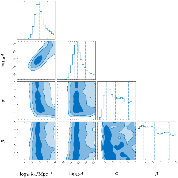
Figure 4: The posteriors on the parameters of the broken power law parameterization (3.4).

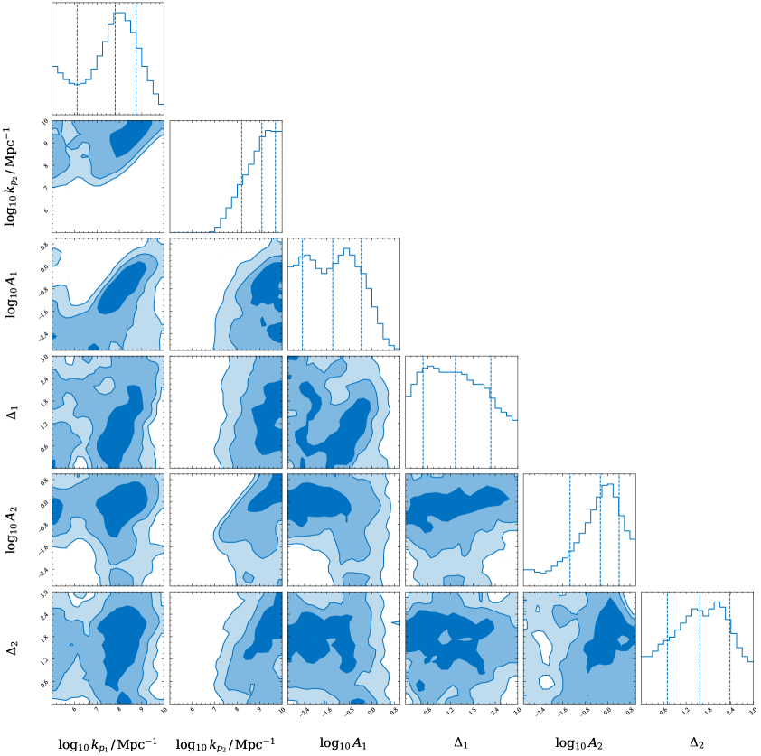
Figure 5: The posteriors on the parameters of the double lognormal parameterization (3.5).

When comparing the results of the double-peak lognormal primordial curvature power spectrum with the single-peak models using $\delta$, box, lognormal, and broken power law forms, the Bayesian analysis yields no support in favor of the single-peak models with respective Bayes factors of $\ln\mathcal{B}=0.29$, $\ln\mathcal{B}=0.26$, $\ln\mathcal{B}=0.46$, and $\ln\mathcal{B}=0.45$. Thus, the PTAs data show no significant evidence for or against the single-peak primordial curvature power spectrum over the double-peak primordial curvature power spectrum. Due to the very close values of logarithmic evidence, it is also difficult to favor which single-peak model provides a better fit.

After obtaining the best-fit values from posteriors, we present the power spectrum of the primordial curvature perturbations in Figure 6 and the corresponding SIGWs in Figure 7. In Figure 6, the orange thin solid line, blue thick solid line, red dashed line, black dotted line, and green dash-dotted line denote the primordial curvature power spectrum with the $\delta$-function, box, lognormal, broken power law, and double-lognormal parameterizations, respectively. The peak scale of these parameterizations is around $k_{p}\sim 10^{8}~{}{\rm Mpc^{-1}}$, and the amplitude of the primordial curvature power spectrum of these parameterizations at the peak is around $A\sim 0.1$.

In Figure 7, the orange thin solid line, blue thick solid line, red dashed line, black dotted line, and green dash-dotted line represent the energy density of the SIGW from the primordial curvature power spectrum with the $\delta$-function, box, lognormal, broken power law, and double-lognormal parameterizations, respectively. If the PTAs data indeed arises from the SIGWs, this PTAs signal can also be detected by space-based detectors in the future. And the parameterizations of the primordial curvature power spectrum can also be distinguished by the space-based detectors.

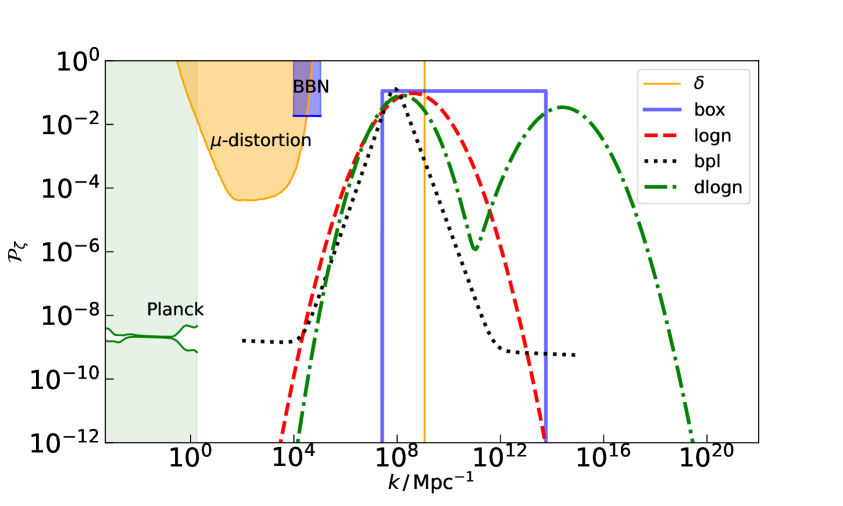
Figure 6: The power spectrum of the primordial curvature perturbation with $\delta$ function, box, lognormal, broken power law, and double lognormal parameterizations by choosing the best-fit parameters value in Table 1. The labels “$\delta$”, “box”, “logn”, “bpl”, and “dlogn” denote $\delta$ function, box, lognormal, broken power law, and double lognormal parameterizations, respectively. The light green shaded region is excluded by the CMB observations [134]. The blue and orange regions are the constraints from the effect on the ratio between neutron and proton during the Big Bang nucleosynthesis (BBN) [140, 141] and $\mu$-distortion of CMB [142, 143], respectively.

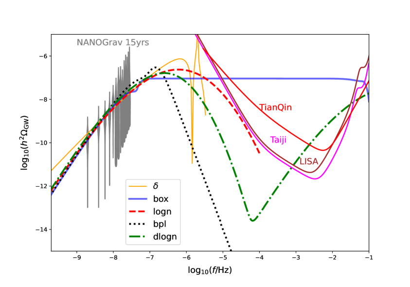
Figure 7: The energy density of SIGWs from the primordial curvature power spectrum parameterizations as displayed in Figure 6. The labels “$\delta$”, “box”, “logn”, “bpl”, and “dlogn” denote $\delta$ function, box, lognormal, broken power law, and double lognormal parameterizations of the primordial curvature power spectrum, respectively. The grey regions represent the results form NANOGrav 15-yr data set [2, 8], the red curve denotes the TianQin sensitivity curve [87], the magenta curve shows the Taiji sensitivity curve [86], the brown curve shows the LISA sensitivity curve [85].

4 Discussion and conclusion

The stochastic signal detected by the NANOGrav, PPTA, EPTA, and CPTA collaborations points to the GW origin and can be explained by the SIGWs, where the scalar perturbations are seeded from the primordial curvature perturbations. To determine the SIGWs model that best fits the observed stochastic signal, we explore both single-peak and double-peak parameterizations for the power spectrum of the primordial curvature perturbations. For the single-peak scenarios, we consider parameterizations using the $\delta$-function form, box form, lognormal form, and broken power law form. Additionally, in the double-peak scenario, we employ the double lognormal form. The best-fit values for the scale and amplitude of the primordial curvature perturbations at the peak, obtained from these five parameterizations, are approximately $k_{p}\sim 10^{8}~{}{\rm Mpc^{-1}}$ and $A\sim 0.1$. More specifically, they are $\log_{10}A=1.28^{+1.79}_{-1.95}$ and $\log_{10}k_{p}/\mathrm{Mpc}^{-1}=11.19^{+1.99}_{-2.26}$ for the $\delta$ function model; $\log_{10}A=-0.95^{+0.52}_{-0.28}$, $\log_{10}k_{\mathrm{min}}/\mathrm{Mpc}^{-1}=7.40^{+0.47}_{-0.31}$ and $\log_{10}k_{\mathrm{max}}/\mathrm{Mpc}^{-1}=13.77^{+4.24}_{-4.11}$ for the box model; $\log_{10}A=-0.88^{+0.81}_{-0.36}$, $\alpha=2.33^{+1.72}_{-1.14}$, $\beta=2.22^{+1.87}_{-1.53}$ and $\log_{10}k_{p}/\mathrm{Mpc}^{-1}=7.91^{+0.88}_{-0.44}$ for the Broken power law model; $\log_{10}A=-0.26^{+0.60}_{-0.58}$, $\Delta=1.66^{+0.65}_{-0.87}$, and $\log_{10}k_{p}/\mathrm{Mpc}^{-1}=8.61^{+0.93}_{-0.79}$ for the lognormal model; $\log_{10}A_{1}=-0.34^{+0.64}_{-0.61}$, $\Delta_{1}=1.32^{+0.77}_{-0.77}$, $\log_{10}k_{p_{1}}/\mathrm{Mpc}^{-1}=8.21^{+0.92}_{-0.66}$, $\log_{10}A_{2}=-0.84^{+1.25}_{-1.49}$, $\Delta_{2}=1.67^{+0.94}_{-1.09}$, $\log_{10}k_{p_{2}}/\mathrm{Mpc}^{-1}=14.40^{+3.75}_{-3.90}$ for the double lognormal model. Comparing the results with the double-peak scenarios, the Bayesian analysis provides no support in favor of the single-peak models, with respective Bayes factors of $\ln\mathcal{B}=0.29$, $\ln\mathcal{B}=0.26$, $\ln\mathcal{B}=0.46$, and $\ln\mathcal{B}=0.45$ for the $\delta$-function, box, lognormal, and broken power law forms, respectively. If the stochastic signal observed by the PTAs indeed originates from SIGWs, it may also be detectable by space-based gravitational wave detectors in the future, potentially allowing for the distinction between different types of SIGWs. Although our analysis in this paper focuses on the double-peak model, our conclusion can be extended to multi-peak models.

When considering the PBHs generated accompanied by SIGWs, there may be a challenge of potentially producing an excessive number of PBHs. One potential solution to address this concern is to take into account non-Gaussianities [10, 11]. This is a critical matter in the context of SIGWs attempting to explain the NANOGrav 15-year data set, and we leave it to future research.

In conclusion, the recent gravitational wave background signal can be explained by SIGWs, without preference for a single peak in the primordial curvature power spectrum over a multi-peak configuration.

References

- [1] NANOGrav collaboration, The NANOGrav 15 yr Data Set: Observations and Timing of 68 Millisecond Pulsars, Astrophys. J. Lett. 951 (2023) L9 [2306.16217].
- [2] NANOGrav collaboration, The NANOGrav 15 yr Data Set: Evidence for a Gravitational-wave Background, Astrophys. J. Lett. 951 (2023) L8 [2306.16213].
- [3] A. Zic et al., The Parkes Pulsar Timing Array Third Data Release, 2306.16230.
- [4] D.J. Reardon et al., Search for an Isotropic Gravitational-wave Background with the Parkes Pulsar Timing Array, Astrophys. J. Lett. 951 (2023) L6 [2306.16215].
- [5] EPTA collaboration, The second data release from the European Pulsar Timing Array I. The dataset and timing analysis, Astron. Astrophys. 678 (2023) A48 [2306.16224].
- [6] EPTA collaboration, The second data release from the European Pulsar Timing Array III. Search for gravitational wave signals, Astron. Astrophys. 678 (2023) A50 [2306.16214].
- [7] H. Xu et al., Searching for the Nano-Hertz Stochastic Gravitational Wave Background with the Chinese Pulsar Timing Array Data Release I, Res. Astron. Astrophys. 23 (2023) 075024 [2306.16216].
- [8] NANOGrav collaboration, The NANOGrav 15 yr Data Set: Search for Signals from New Physics, Astrophys. J. Lett. 951 (2023) L11 [2306.16219].
- [9] EPTA collaboration, The second data release from the European Pulsar Timing Array: V. Implications for massive black holes, dark matter and the early Universe, 2306.16227.
- [10] G. Franciolini, A. Iovino, Junior., V. Vaskonen and H. Veermae, The recent gravitational wave observation by pulsar timing arrays and primordial black holes: the importance of non-gaussianities, 2306.17149.
- [11] L. Liu, Z.-C. Chen and Q.-G. Huang, Implications for the non-Gaussianity of curvature perturbation from pulsar timing arrays, 2307.01102.
- [12] S. Vagnozzi, Inflationary interpretation of the stochastic gravitational wave background signal detected by pulsar timing array experiments, JHEAp 39 (2023) 81 [2306.16912].
- [13] Y.-F. Cai, X.-C. He, X. Ma, S.-F. Yan and G.-W. Yuan, Limits on scalar-induced gravitational waves from the stochastic background by pulsar timing array observations, 2306.17822.
- [14] S. Wang, Z.-C. Zhao, J.-P. Li and Q.-H. Zhu, Implications of Pulsar Timing Array Data for Scalar-Induced Gravitational Waves and Primordial Black Holes: Primordial Non-Gaussianity Considered, 2307.00572.
- [15] Z. Yi, Q. Gao, Y. Gong, Y. Wang and F. Zhang, The waveform of the scalar induced gravitational waves in light of Pulsar Timing Array data, 2307.02467.
- [16] Y.-C. Bi, Y.-M. Wu, Z.-C. Chen and Q.-G. Huang, Implications for the Supermassive Black Hole Binaries from the NANOGrav 15-year Data Set, 2307.00722.
- [17] Y.-M. Wu, Z.-C. Chen and Q.-G. Huang, Cosmological Interpretation for the Stochastic Signal in Pulsar Timing Arrays, 2307.03141.
- [18] S. Wang, Z.-C. Zhao and Q.-H. Zhu, Constraints On Scalar-Induced Gravitational Waves Up To Third Order From Joint Analysis of BBN, CMB, And PTA Data, 2307.03095.
- [19] G. Franciolini, D. Racco and F. Rompineve, Footprints of the QCD Crossover on Cosmological Gravitational Waves at Pulsar Timing Arrays, 2306.17136.
- [20] J.-H. Jin, Z.-C. Chen, Z. Yi, Z.-Q. You, L. Liu and Y. Wu, Confronting sound speed resonance with pulsar timing arrays, JCAP 09 (2023) 016 [2307.08687].
- [21] L. Liu, Z.-C. Chen and Q.-G. Huang, Probing the equation of state of the early Universe with pulsar timing arrays, 2307.14911.
- [22] Z. Yi, Z.-Q. You, Y. Wu, Z.-C. Chen and L. Liu, Exploring the NANOGrav Signal and Planet-mass Primordial Black Holes through Higgs Inflation, 2308.14688.
- [23] Z. Yi, Z.-Q. You and Y. Wu, Model-independent reconstruction of the primordial curvature power spectrum from PTA data, 2308.05632.
- [24] Z.-Q. You, Z. Yi and Y. Wu, Constraints on primordial curvature power spectrum with pulsar timing arrays, 2307.04419.
- [25] Y.-M. Wu, Z.-C. Chen, Y.-C. Bi and Q.-G. Huang, Constraining the Graviton Mass with the NANOGrav 15-Year Data Set, 2310.07469.
- [26] Y.-C. Bi, Y.-M. Wu, Z.-C. Chen and Q.-G. Huang, Constraints on the velocity of gravitational waves from NANOGrav 15-year data set, 2310.08366.
- [27] Z.-C. Chen, Y.-M. Wu, Y.-C. Bi and Q.-G. Huang, Search for Non-Tensorial Gravitational-Wave Backgrounds in the NANOGrav 15-Year Data Set, 2310.11238.
- [28] L. Liu, Y. Wu and Z.-C. Chen, Simultaneously probing the sound speed and equation of state of the early Universe with pulsar timing arrays, 2310.16500.
- [29] Y.B. Zel’dovich and I.D. Novikov, The Hypothesis of Cores Retarded during Expansion and the Hot Cosmological Model, Soviet Astron. AJ (Engl. Transl. ), 10 (1967) 602.
- [30] S. Hawking, Gravitationally collapsed objects of very low mass, Mon. Not. Roy. Astron. Soc. 152 (1971) 75.
- [31] B.J. Carr and S.W. Hawking, Black holes in the early Universe, Mon. Not. Roy. Astron. Soc. 168 (1974) 399.
- [32] Z.-C. Chen and Q.-G. Huang, Merger Rate Distribution of Primordial-Black-Hole Binaries, Astrophys. J. 864 (2018) 61 [1801.10327].
- [33] Z.-C. Chen, F. Huang and Q.-G. Huang, Stochastic Gravitational-wave Background from Binary Black Holes and Binary Neutron Stars and Implications for LISA, Astrophys. J. 871 (2019) 97 [1809.10360].
- [34] L. Liu, Z.-K. Guo and R.-G. Cai, Effects of the surrounding primordial black holes on the merger rate of primordial black hole binaries, Phys. Rev. D 99 (2019) 063523 [1812.05376].
- [35] L. Liu, Z.-K. Guo and R.-G. Cai, Effects of the merger history on the merger rate density of primordial black hole binaries, Eur. Phys. J. C 79 (2019) 717 [1901.07672].
- [36] Z.-C. Chen and Q.-G. Huang, Distinguishing Primordial Black Holes from Astrophysical Black Holes by Einstein Telescope and Cosmic Explorer, JCAP 08 (2020) 039 [1904.02396].
- [37] L. Liu, Z.-K. Guo, R.-G. Cai and S.P. Kim, Merger rate distribution of primordial black hole binaries with electric charges, Phys. Rev. D 102 (2020) 043508 [2001.02984].
- [38] L. Liu, O. Christiansen, Z.-K. Guo, R.-G. Cai and S.P. Kim, Gravitational and electromagnetic radiation from binary black holes with electric and magnetic charges: Circular orbits on a cone, Phys. Rev. D 102 (2020) 103520 [2008.02326].
- [39] L. Liu, O. Christiansen, W.-H. Ruan, Z.-K. Guo, R.-G. Cai and S.P. Kim, Gravitational and electromagnetic radiation from binary black holes with electric and magnetic charges: elliptical orbits on a cone, Eur. Phys. J. C 81 (2021) 1048 [2011.13586].
- [40] Y. Wu, Merger history of primordial black-hole binaries, Phys. Rev. D 101 (2020) 083008 [2001.03833].
- [41] Z.-C. Chen, C. Yuan and Q.-G. Huang, Confronting the primordial black hole scenario with the gravitational-wave events detected by LIGO-Virgo, Phys. Lett. B 829 (2022) 137040 [2108.11740].
- [42] L. Liu and S.P. Kim, Merger rate of charged black holes from the two-body dynamical capture, JCAP 03 (2022) 059 [2201.02581].
- [43] Z.-C. Chen, S.-S. Du, Q.-G. Huang and Z.-Q. You, Constraints on primordial-black-hole population and cosmic expansion history from GWTC-3, JCAP 03 (2023) 024 [2205.11278].
- [44] Z.-C. Chen, S.P. Kim and L. Liu, Gravitational and electromagnetic radiation from binary black holes with electric and magnetic charges: hyperbolic orbits on a cone, Commun. Theor. Phys. 75 (2023) 065401 [2210.15564].
- [45] L. Liu, Z.-Q. You, Y. Wu and Z.-C. Chen, Constraining the merger history of primordial-black-hole binaries from GWTC-3, Phys. Rev. D 107 (2023) 063035 [2210.16094].
- [46] L.-M. Zheng, Z. Li, Z.-C. Chen, H. Zhou and Z.-H. Zhu, Towards a reliable reconstruction of the power spectrum of primordial curvature perturbation on small scales from GWTC-3, Phys. Lett. B 838 (2023) 137720 [2212.05516].
- [47] Z. Yi and Q. Fei, Constraints on primordial curvature spectrum from primordial black holes and scalar-induced gravitational waves, Eur. Phys. J. C 83 (2023) 82 [2210.03641].
- [48] X.-J. Zhu, W. Cui and E. Thrane, The minimum and maximum gravitational-wave background from supermassive binary black holes, Mon. Not. Roy. Astron. Soc. 482 (2019) 2588 [1806.02346].
- [49] J. Li, Z.-C. Chen and Q.-G. Huang, Measuring the tilt of primordial gravitational-wave power spectrum from observations, Sci. China Phys. Mech. Astron. 62 (2019) 110421 [1907.09794].
- [50] Z.-C. Chen, C. Yuan and Q.-G. Huang, Non-tensorial gravitational wave background in NANOGrav 12.5-year data set, Sci. China Phys. Mech. Astron. 64 (2021) 120412 [2101.06869].
- [51] Y.-M. Wu, Z.-C. Chen and Q.-G. Huang, Constraining the Polarization of Gravitational Waves with the Parkes Pulsar Timing Array Second Data Release, Astrophys. J. 925 (2022) 37 [2108.10518].
- [52] Z.-C. Chen, Y.-M. Wu and Q.-G. Huang, Searching for isotropic stochastic gravitational-wave background in the international pulsar timing array second data release, Commun. Theor. Phys. 74 (2022) 105402 [2109.00296].
- [53] Z.-C. Chen, Y.-M. Wu and Q.-G. Huang, Search for the Gravitational-wave Background from Cosmic Strings with the Parkes Pulsar Timing Array Second Data Release, Astrophys. J. 936 (2022) 20 [2205.07194].
- [54] PPTA collaboration, Constraining ultralight vector dark matter with the Parkes Pulsar Timing Array second data release, Phys. Rev. D 106 (2022) L081101 [2210.03880].
- [55] IPTA collaboration, Searching for continuous Gravitational Waves in the second data release of the International Pulsar Timing Array, Mon. Not. Roy. Astron. Soc. 521 (2023) 5077 [2303.10767].
- [56] Y.-M. Wu, Z.-C. Chen and Q.-G. Huang, Search for stochastic gravitational-wave background from massive gravity in the NANOGrav 12.5-year dataset, Phys. Rev. D 107 (2023) 042003 [2302.00229].
- [57] Y.-M. Wu, Z.-C. Chen and Q.-G. Huang, Pulsar timing residual induced by ultralight tensor dark matter, JCAP 09 (2023) 021 [2305.08091].
- [58] International Pulsar Timing Array collaboration, Comparing recent PTA results on the nanohertz stochastic gravitational wave background, 2309.00693.
- [59] Z.-C. Chen, Q.-G. Huang, C. Liu, L. Liu, X.-J. Liu, Y. Wu et al., Prospects for Taiji to detect a gravitational-wave background from cosmic strings, 2310.00411.
- [60] K. Tomita, Non-linear theory of gravitational instability in the expanding universe, Progress of Theoretical Physics 37 (1967) 831.
- [61] R. Saito and J. Yokoyama, Gravitational wave background as a probe of the primordial black hole abundance, Phys. Rev. Lett. 102 (2009) 161101 [0812.4339].
- [62] S. Young, C.T. Byrnes and M. Sasaki, Calculating the mass fraction of primordial black holes, JCAP 07 (2014) 045 [1405.7023].
- [63] C. Yuan, Z.-C. Chen and Q.-G. Huang, Probing primordial–black-hole dark matter with scalar induced gravitational waves, Phys. Rev. D 100 (2019) 081301 [1906.11549].
- [64] C. Yuan, Z.-C. Chen and Q.-G. Huang, Log-dependent slope of scalar induced gravitational waves in the infrared regions, Phys. Rev. D 101 (2020) 043019 [1910.09099].
- [65] Z.-C. Chen, C. Yuan and Q.-G. Huang, Pulsar Timing Array Constraints on Primordial Black Holes with NANOGrav 11-Year Dataset, Phys. Rev. Lett. 124 (2020) 251101 [1910.12239].
- [66] C. Yuan, Z.-C. Chen and Q.-G. Huang, Scalar induced gravitational waves in different gauges, Phys. Rev. D 101 (2020) 063018 [1912.00885].
- [67] K.N. Ananda, C. Clarkson and D. Wands, The Cosmological gravitational wave background from primordial density perturbations, Phys. Rev. D 75 (2007) 123518 [gr-qc/0612013].
- [68] D. Baumann, P.J. Steinhardt, K. Takahashi and K. Ichiki, Gravitational Wave Spectrum Induced by Primordial Scalar Perturbations, Phys. Rev. D 76 (2007) 084019 [hep-th/0703290].
- [69] L. Alabidi, K. Kohri, M. Sasaki and Y. Sendouda, Observable Spectra of Induced Gravitational Waves from Inflation, JCAP 09 (2012) 017 [1203.4663].
- [70] T. Nakama, J. Silk and M. Kamionkowski, Stochastic gravitational waves associated with the formation of primordial black holes, Phys. Rev. D 95 (2017) 043511 [1612.06264].
- [71] K. Kohri and T. Terada, Semianalytic calculation of gravitational wave spectrum nonlinearly induced from primordial curvature perturbations, Phys. Rev. D 97 (2018) 123532 [1804.08577].
- [72] S.-L. Cheng, W. Lee and K.-W. Ng, Primordial black holes and associated gravitational waves in axion monodromy inflation, JCAP 07 (2018) 001 [1801.09050].
- [73] R.-G. Cai, S. Pi, S.-J. Wang and X.-Y. Yang, Resonant multiple peaks in the induced gravitational waves, JCAP 05 (2019) 013 [1901.10152].
- [74] R.-g. Cai, S. Pi and M. Sasaki, Gravitational Waves Induced by non-Gaussian Scalar Perturbations, Phys. Rev. Lett. 122 (2019) 201101 [1810.11000].
- [75] R.-G. Cai, S. Pi, S.-J. Wang and X.-Y. Yang, Pulsar Timing Array Constraints on the Induced Gravitational Waves, JCAP 10 (2019) 059 [1907.06372].
- [76] R.-G. Cai, Z.-K. Guo, J. Liu, L. Liu and X.-Y. Yang, Primordial black holes and gravitational waves from parametric amplification of curvature perturbations, JCAP 06 (2020) 013 [1912.10437].
- [77] R.-G. Cai, Y.-C. Ding, X.-Y. Yang and Y.-F. Zhou, Constraints on a mixed model of dark matter particles and primordial black holes from the galactic 511 keV line, JCAP 03 (2021) 057 [2007.11804].
- [78] S. Pi and M. Sasaki, Gravitational Waves Induced by Scalar Perturbations with a Lognormal Peak, JCAP 09 (2020) 037 [2005.12306].
- [79] G. Domènech, S. Pi and M. Sasaki, Induced gravitational waves as a probe of thermal history of the universe, JCAP 08 (2020) 017 [2005.12314].
- [80] L. Liu, X.-Y. Yang, Z.-K. Guo and R.-G. Cai, Testing primordial black hole and measuring the Hubble constant with multiband gravitational-wave observations, JCAP 01 (2023) 006 [2112.05473].
- [81] T. Papanikolaou, C. Tzerefos, S. Basilakos and E.N. Saridakis, Scalar induced gravitational waves from primordial black hole Poisson fluctuations in f(R) gravity, JCAP 10 (2022) 013 [2112.15059].
- [82] T. Papanikolaou, C. Tzerefos, S. Basilakos and E.N. Saridakis, No constraints for f(T) gravity from gravitational waves induced from primordial black hole fluctuations, Eur. Phys. J. C 83 (2023) 31 [2205.06094].
- [83] D.-S. Meng, C. Yuan and Q.-G. Huang, Primordial black holes generated by the non-minimal spectator field, Sci. China Phys. Mech. Astron. 66 (2023) 280411 [2212.03577].
- [84] K. Danzmann, LISA: An ESA cornerstone mission for a gravitational wave observatory, Class. Quant. Grav. 14 (1997) 1399.
- [85] LISA collaboration, Laser Interferometer Space Antenna, 1702.00786.
- [86] W.-R. Hu and Y.-L. Wu, The Taiji Program in Space for gravitational wave physics and the nature of gravity, Natl. Sci. Rev. 4 (2017) 685.
- [87] TianQin collaboration, TianQin: a space-borne gravitational wave detector, Class. Quant. Grav. 33 (2016) 035010 [1512.02076].
- [88] Y. Gong, J. Luo and B. Wang, Concepts and status of Chinese space gravitational wave detection projects, Nature Astron. 5 (2021) 881 [2109.07442].
- [89] S. Kawamura et al., The Japanese space gravitational wave antenna: DECIGO, Class. Quant. Grav. 28 (2011) 094011.
- [90] Planck collaboration, Planck 2018 results. X. Constraints on inflation, Astron. Astrophys. 641 (2020) A10 [1807.06211].
- [91] J. Martin, H. Motohashi and T. Suyama, Ultra Slow-Roll Inflation and the non-Gaussianity Consistency Relation, Phys. Rev. D 87 (2013) 023514 [1211.0083].
- [92] H. Motohashi, A.A. Starobinsky and J. Yokoyama, Inflation with a constant rate of roll, JCAP 09 (2015) 018 [1411.5021].
- [93] Z. Yi and Y. Gong, On the constant-roll inflation, JCAP 03 (2018) 052 [1712.07478].
- [94] J. Garcia-Bellido and E. Ruiz Morales, Primordial black holes from single field models of inflation, Phys. Dark Univ. 18 (2017) 47 [1702.03901].
- [95] C. Germani and T. Prokopec, On primordial black holes from an inflection point, Phys. Dark Univ. 18 (2017) 6 [1706.04226].
- [96] H. Motohashi and W. Hu, Primordial Black Holes and Slow-Roll Violation, Phys. Rev. D 96 (2017) 063503 [1706.06784].
- [97] J.M. Ezquiaga, J. Garcia-Bellido and E. Ruiz Morales, Primordial Black Hole production in Critical Higgs Inflation, Phys. Lett. B 776 (2018) 345 [1705.04861].
- [98] H. Di and Y. Gong, Primordial black holes and second order gravitational waves from ultra-slow-roll inflation, JCAP 07 (2018) 007 [1707.09578].
- [99] G. Ballesteros, J. Beltran Jimenez and M. Pieroni, Black hole formation from a general quadratic action for inflationary primordial fluctuations, JCAP 06 (2019) 016 [1811.03065].
- [100] I. Dalianis, A. Kehagias and G. Tringas, Primordial black holes from -attractors, JCAP 01 (2019) 037 [1805.09483].
- [101] F. Bezrukov, M. Pauly and J. Rubio, On the robustness of the primordial power spectrum in renormalized Higgs inflation, JCAP 02 (2018) 040 [1706.05007].
- [102] K. Kannike, L. Marzola, M. Raidal and H. Veermäe, Single Field Double Inflation and Primordial Black Holes, JCAP 09 (2017) 020 [1705.06225].
- [103] J. Lin, Q. Gao, Y. Gong, Y. Lu, C. Zhang and F. Zhang, Primordial black holes and secondary gravitational waves from and inflation, Phys. Rev. D 101 (2020) 103515 [2001.05909].
- [104] J. Lin, S. Gao, Y. Gong, Y. Lu, Z. Wang and F. Zhang, Primordial black holes and scalar induced gravitational waves from Higgs inflation with noncanonical kinetic term, Phys. Rev. D 107 (2023) 043517 [2111.01362].
- [105] Q. Gao, Y. Gong and Z. Yi, On the constant-roll inflation with large and small , Universe 5 (2019) 215 [1901.04646].
- [106] Q. Gao, Y. Gong and Z. Yi, Primordial black holes and secondary gravitational waves from natural inflation, Nucl. Phys. B 969 (2021) 115480 [2012.03856].
- [107] Q. Gao, Primordial black holes and secondary gravitational waves from chaotic inflation, Sci. China Phys. Mech. Astron. 64 (2021) 280411 [2102.07369].
- [108] Z. Yi, Y. Gong, B. Wang and Z.-h. Zhu, Primordial black holes and secondary gravitational waves from the Higgs field, Phys. Rev. D 103 (2021) 063535 [2007.09957].
- [109] Z. Yi, Q. Gao, Y. Gong and Z.-h. Zhu, Primordial black holes and scalar-induced secondary gravitational waves from inflationary models with a noncanonical kinetic term, Phys. Rev. D 103 (2021) 063534 [2011.10606].
- [110] Z. Yi and Z.-H. Zhu, NANOGrav signal and LIGO-Virgo primordial black holes from the Higgs field, JCAP 05 (2022) 046 [2105.01943].
- [111] Z. Yi, Primordial black holes and scalar-induced gravitational waves from the generalized Brans-Dicke theory, JCAP 03 (2023) 048 [2206.01039].
- [112] F. Zhang, Y. Gong, J. Lin, Y. Lu and Z. Yi, Primordial non-Gaussianity from G-inflation, JCAP 04 (2021) 045 [2012.06960].
- [113] S. Pi, Y.-l. Zhang, Q.-G. Huang and M. Sasaki, Scalaron from -gravity as a heavy field, JCAP 05 (2018) 042 [1712.09896].
- [114] A.Y. Kamenshchik, A. Tronconi, T. Vardanyan and G. Venturi, Non-Canonical Inflation and Primordial Black Holes Production, Phys. Lett. B 791 (2019) 201 [1812.02547].
- [115] C. Fu, P. Wu and H. Yu, Primordial Black Holes from Inflation with Nonminimal Derivative Coupling, Phys. Rev. D 100 (2019) 063532 [1907.05042].
- [116] C. Fu, P. Wu and H. Yu, Scalar induced gravitational waves in inflation with gravitationally enhanced friction, Phys. Rev. D 101 (2020) 023529 [1912.05927].
- [117] I. Dalianis, S. Karydas and E. Papantonopoulos, Generalized Non-Minimal Derivative Coupling: Application to Inflation and Primordial Black Hole Production, JCAP 06 (2020) 040 [1910.00622].
- [118] A. Gundhi and C.F. Steinwachs, Scalaron–Higgs inflation reloaded: Higgs-dependent scalaron mass and primordial black hole dark matter, Eur. Phys. J. C 81 (2021) 460 [2011.09485].
- [119] D.Y. Cheong, S.M. Lee and S.C. Park, Primordial black holes in Higgs- inflation as the whole of dark matter, JCAP 01 (2021) 032 [1912.12032].
- [120] F. Zhang, Primordial black holes and scalar induced gravitational waves from the E model with a Gauss-Bonnet term, Phys. Rev. D 105 (2022) 063539 [2112.10516].
- [121] F. Zhang, J. Lin and Y. Lu, Double-peaked inflation model: Scalar induced gravitational waves and primordial-black-hole suppression from primordial non-Gaussianity, Phys. Rev. D 104 (2021) 063515 [2106.10792].
- [122] S. Kawai and J. Kim, Primordial black holes from Gauss-Bonnet-corrected single field inflation, Phys. Rev. D 104 (2021) 083545 [2108.01340].
- [123] R.-G. Cai, C. Chen and C. Fu, Primordial black holes and stochastic gravitational wave background from inflation with a noncanonical spectator field, Phys. Rev. D 104 (2021) 083537 [2108.03422].
- [124] P. Chen, S. Koh and G. Tumurtushaa, Primordial black holes and induced gravitational waves from inflation in the Horndeski theory of gravity, 2107.08638.
- [125] R. Zheng, J. Shi and T. Qiu, On primordial black holes and secondary gravitational waves generated from inflation with solo/multi-bumpy potential *, Chin. Phys. C 46 (2022) 045103 [2106.04303].
- [126] A. Karam, N. Koivunen, E. Tomberg, V. Vaskonen and H. Veermäe, Anatomy of single-field inflationary models for primordial black holes, JCAP 03 (2023) 013 [2205.13540].
- [127] A. Ashoorioon, A. Rostami and J.T. Firouzjaee, EFT compatible PBHs: effective spawning of the seeds for primordial black holes during inflation, JHEP 07 (2021) 087 [1912.13326].
- [128] K.A. Malik and D. Wands, Cosmological perturbations, Phys. Rept. 475 (2009) 1 [0809.4944].
- [129] J.R. Espinosa, D. Racco and A. Riotto, A Cosmological Signature of the SM Higgs Instability: Gravitational Waves, JCAP 09 (2018) 012 [1804.07732].
- [130] Y. Lu, Y. Gong, Z. Yi and F. Zhang, Constraints on primordial curvature perturbations from primordial black hole dark matter and secondary gravitational waves, JCAP 12 (2019) 031 [1907.11896].
- [131] K. Ando, K. Inomata, M. Kawasaki, K. Mukaida and T.T. Yanagida, Primordial black holes for the LIGO events in the axionlike curvaton model, Phys. Rev. D 97 (2018) 123512 [1711.08956].
- [132] V. Vaskonen and H. Veermäe, Did NANOGrav see a signal from primordial black hole formation?, Phys. Rev. Lett. 126 (2021) 051303 [2009.07832].
- [133] V. De Luca, G. Franciolini and A. Riotto, NANOGrav Data Hints at Primordial Black Holes as Dark Matter, Phys. Rev. Lett. 126 (2021) 041303 [2009.08268].
- [134] Planck collaboration, Planck 2018 results. X. Constraints on inflation, Astron. Astrophys. 641 (2020) A10 [1807.06211].
- [135] G. Ashton et al., BILBY: A user-friendly Bayesian inference library for gravitational-wave astronomy, Astrophys. J. Suppl. 241 (2019) 27 [1811.02042].
- [136] J. Skilling, Nested sampling, AIP Conf. Proc. (2004) 395.
- [137] C.J. Moore and A. Vecchio, Ultra-low-frequency gravitational waves from cosmological and astrophysical processes, Nature Astron. 5 (2021) 1268 [2104.15130].
- [138] W.G. Lamb, S.R. Taylor and R. van Haasteren, The Need For Speed: Rapid Refitting Techniques for Bayesian Spectral Characterization of the Gravitational Wave Background Using PTAs, 2303.15442.
- [139] EPTA collaboration, Practical approaches to analyzing PTA data: Cosmic strings with six pulsars, 2306.12234.
- [140] D. Jeong, J. Pradler, J. Chluba and M. Kamionkowski, Silk damping at a redshift of a billion: a new limit on small-scale adiabatic perturbations, Phys. Rev. Lett. 113 (2014) 061301 [1403.3697].
- [141] K. Inomata, M. Kawasaki and Y. Tada, Revisiting constraints on small scale perturbations from big-bang nucleosynthesis, Phys. Rev. D 94 (2016) 043527 [1605.04646].
- [142] D.J. Fixsen, E.S. Cheng, J.M. Gales, J.C. Mather, R.A. Shafer and E.L. Wright, The Cosmic Microwave Background spectrum from the full COBE FIRAS data set, Astrophys. J. 473 (1996) 576 [astro-ph/9605054].
- [143] J. Chluba, A.L. Erickcek and I. Ben-Dayan, Probing the inflaton: Small-scale power spectrum constraints from measurements of the CMB energy spectrum, Astrophys. J. 758 (2012) 76 [1203.2681].