Fairness-aware Federated Minimax Optimization with Convergence Guarantee

Abstract

Federated learning (FL) has garnered considerable attention due to its privacy-preserving feature. Nonetheless, the lack of freedom in managing user data can lead to group fairness issues, where models are biased towards sensitive factors such as race or gender. To tackle this issue, this paper proposes a novel algorithm, fair federated averaging with augmented Lagrangian method (FFALM), designed explicitly to address group fairness issues in FL. Specifically, we impose a fairness constraint on the training objective and solve the minimax reformulation of the constrained optimization problem. Then, we derive the theoretical upper bound for the convergence rate of FFALM. The effectiveness of FFALM in improving fairness is shown empirically on CelebA and UTKFace datasets in the presence of severe statistical heterogeneity.

I Introduction

Federated learning (FL) [1] is a distributed machine learning approach that enables model training on potentially sensitive data from different entities without the necessity for data sharing. This technique is promising in diverse domains such as computer vision (CV) as it can facilitate training of models on a large-scale, diverse set of data while preserving data privacy. However, a direct implementation of existing federated algorithms may violate group fairness [2], which refers to the equitable treatment of different groups in a population. Group fairness is required by law such as in Europe [3], enforcing that the decision making by predictive models does not exhibit bias towards any particular sensitive group, such as race or gender. For example, an AI model used in a hiring process may have been trained on historical data that reflects biased hiring patterns, leading to discriminatory outcomes for underrepresented groups in the workforce. There are more examples [4] that further motivate raising awareness in training fair deep learning models.

The sources of group unfairness or bias mainly come from dataset, which may reflect measurement or historical bias from the annotators, and the training algorithm, which may learn unwanted biased features from such dataset. The aforementioned sources also induce statistical heterogeneity. Under severe heterogeneity, the trained model may have poor task performance and biased model. Finding FL algorithms that are fair and robust to statistical heterogeneity or non-identical and independently distributed (non-iid) data is an arduous task, and currently it is an open problem [5].

I-A Contributions

Since we have little control on the clients data in FL, efforts to mitigate bias from the training algorithm are important. Therefore, the focus of this paper is to improve group fairness in binary classification tasks involving binary sensitive attributes, which cover most practical applications [6]. In particular, we propose a new federated algorithm that is effective in reducing bias while maintaining similar task performance as existing federated algorithms. The main contributions are summarized below.

• We propose a fairness-aware algorithm, fair federated averaging with augmented Lagrangian method (FFALM). Firstly, we formulate a constrained minimization problem on the global loss function satisfying a fairness metric. Inspired by augmented Lagrangian method [7], we solve the problem by leveraging the local training as a sub-solver to find the optimal model parameter given a dual iterate. The dual iterates from the clients are aggregated using weighted average.

• We reformulate the objective as a minimax optimization and propose a theoretical upper bound for the convergence rate of FFALM over a nonconvex-strongly-concave objective function, which is $\mathcal{O}(\frac{1}{T^{2/3}})$.

• We empirically assess the proposed method on widely used CV datasets (CelebA and UTKFace). Experimental results show that FFALM improves fairness by $14\%$ in the attractiveness prediction task and by $6\%$ in the youth prediction task over the baselines under severe data heterogeneity.

II Related Work

There have been some engaging results in tackling the fairness issues in deep-learning models. In the following, we categorize some prior related works based on how the training is conducted, either centralized or federated.

II-A Ensuring fairness in centralized learning

In centralized learning, it is not uncommon to modify the training framework to achieve a suitable degree of group fairness. The authors of [8] decorrelated the input images and the protected group attributes by using adversarial training. Knowledge transfer techniques and multi-classifiers can also be adopted as a debiasing method [9]. Augmenting each image sample with its perturbed version generated from generative models can potentially reduce biases as well [10]. The aforementioned works require additional components to the model, thus increasing the computation cost. This might not be suitable for FL. A possible alternative is to alter the loss function to take into account group fairness. The authors of [11] introduced a loss function obtained from the upper bound of the Lagrangian based on a constrained optimization formulation from a finite hypothesis space perspective.

II-B Ensuring fairness in FL

Some prior works considered group fairness in FL. Due to system constraints, most innovations came from the objective formulation to include fairness or more information exchange between the server and the clients. The example for the latter is FairFed [12], where the client coefficients are adaptively adjusted during the aggregation phase based on the deviation of each client’s fairness metric from the global average. Along the line of the objective formulation, FCFL [13] proposed a two-stage optimization to solve a multi-objective optimization with fairness constraints, which demands more communication rounds. FPFL [14] utilized differential multipliers to solve a constrained optimization problem, which is similar to this work. FedFB [15] adjusted the weight of the local loss function for each sensitive group during the aggregation phase. While the constraints formulation in FPFL involve overall loss function, this work has one constraint which enforces the equality of losses evaluated on each sensitive attribute. Moreover, the theoretical convergence guarantee is missing for the aforementioned works.

III Preliminaries

In this section, we introduce some mathematical notations and group fairness notions. After that, we briefly describe the problem formulation and the minimax framework of FL.

III-A Notations

Throughout this paper, we primarily focus on supervised binary classification tasks with binary sensitive attributes. The dataset is denoted as $\mathcal{D}=X\times Y\times S$ with size $|\mathcal{D}|$ constituting of an input image $X$, a label $Y=\{0,1\}$, and a sensitive attribute $S=\{0,1\}$. We slightly abuse the notation of $\mathcal{D}$, $X$, $Y$, and $S$ to represent both the set and the distribution. The datasets can also be partitioned based on sensitive attributes, $\mathcal{D}^{s_{0}}=X\times Y\times S_{0}$ and $\mathcal{D}^{s_{1}}=X\times Y\times S_{1}$.

Some mathematical notations are stated as follows. $[N]$ denotes $\{1,2,...,N\}$, $\|.\|$ represents the $\ell_{2}$-norm, and $\mathbbm{1}$ denotes the indicator function. We use $\mathcal{W}\subseteq\mathbb{R}^{d}$ and $\Lambda$ to represent the parameter spaces of the model $w$ and an additional training parameter $\lambda$, respectively. Denote $f_{w}:X\rightarrow Y$ as a deep-learning model parameterized by $w$, taking $X$ as an input, and outputting the predicted label $Y$.

III-B Group Fairness Metrics

To evaluate the group fairness performance of a machine learning model $f$, there are various notions based on how likely the model predicts a favorable outcome ($Y=1$) for each group. Demographic parity (DP) [16] is commonly used for assessing the fairness of the model. $f$ satisfies DP if the model prediction $\hat{Y}=f\circ X$ is independent of $S$, i.e.,

$$\forall y\in Y=\{0,1\}\quad\mathbb{P}[\hat{Y}=y|S=0]=\mathbb{P}[\hat{Y}=y|S=1].$$ (1)

Another way to define the notion of group fairness is accuracy parity (AP) [17]. To satisfy this notion, $f$ conforms to the following equality

$$\forall y\in Y=\{0,1\}\quad\mathbb{E}_{\mathcal{D}^{s_{0}}}[\mathbbm{1}_{f(X)\neq Y}]=\mathbb{E}_{\mathcal{D}^{s_{1}}}[\mathbbm{1}_{f(X)\neq Y}].$$ (2)

In some use cases where the preference of users belonging to a sensitive group is considered, it is amenable to adopt equal opportunity (EO) [18] of positive outcomes for each sensitive attribute as a fairness notion, mathematically written as

$$\mathbb{P}[\hat{Y}=1|S=0,Y=1]=\mathbb{P}[\hat{Y}=1|S=1,Y=1].$$ (3)

In practice, it is difficult to achieve perfect fairness imposed by aforementioned fairness notions. To measure how close $f$ is to satisfy DP, we employ demographic parity difference metric $(\Delta_{DP})$ on positive label $(Y=1)$, which is defined as

$$\Delta_{DP}=|\mathbb{E}_{X|S=0}[\mathbbm{1}_{f(X)=1}]-\mathbb{E}_{X|S=1}[\mathbbm{1}_{f(X)=1}]|.$$ (4)

Similarly, the closeness measure to satisfy EO condition, equal opportunity difference ($\Delta_{EO}$) is defined as

$$\Delta_{EO}=|\mathbb{E}_{X|Y=1,S=0}[\mathbbm{1}_{f(X)=1}]-\mathbb{E}_{X|Y=1,S=1}[\mathbbm{1}_{f(X)=1}]|.$$ (5)

These two closeness metrics are commonly used for assessing group fairness in machine learning models. Since only samples rather than the true data distribution are available, the metrics are estimated using the samples.

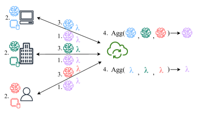
Figure 1: The general FL framework with additional parameter exchange between the server and the clients. In each communication round, there are four steps in FL training: 1. Broadcasting phase 2. Local training phase 3. Client-to-server communication phase 4. Aggregation phase.

III-C Minimax FL Framework

For a FL system with $N$ clients and one server, the goal is to train a global deep learning model $f_{w}$ on each client dataset $\mathcal{D}_{i}$ $(i\in[N])$ without sharing their datasets. In addition, a dual variable $\lambda\in\Lambda$ that aids the training can be exchanged between the server and clients, and processed on the client during local training and on the server during aggregation. The general framework of FL consists of four phases. Firstly, the clients receive the global model from the server (broadcasting phase) and train the model on their own dataset (local training phase). After that, the clients send their model update and the dual parameter update to the server (client-to-server communication phase), and the server aggregates the received updates from each participating client to get an updated model (aggregation phase). This process is repeated until convergence or a specified communication round, as illustrated in Fig. 1.

During local training phase, each client aims to minimize a local loss function on their model and dataset. For any regularization-based federated algorithms, the explicit formulation for the true local risk function of the $i-$th client represented by a loss function $l(f_{w}(x),y)=l(x,y;w)$ and a regularization function $g$ is given by

$$F_{i}(w,\lambda):=\mathbb{E}_{(x_{j},y_{j})\sim\mathcal{D}_{i}}l(x_{j},y_{j};w)+g(\mathcal{D}_{i};\lambda,w),$$ (6)

and the corresponding empirical risk function is given by

$$F_{i,S}(w,\lambda):=\frac{1}{|\mathcal{D}_{i}|}\sum_{(x_{j},y_{j})\sim\mathcal{D}_{i}}l(x_{j},y_{j};w)+g(\mathcal{D}_{i};\lambda,w).$$ (7)

The ultimate goal is to solve the following minimax objective of the true global risk function $F(w,\lambda)$

$$\min_{w}\max_{\lambda}F(w,\lambda):=\sum_{i=1}^{N}p_{i}F_{i}(w,\lambda),$$ (8)

where $p_{i}$ is the client coefficient with $\sum_{i=1}^{N}p_{i}=1$ and $p_{i}\in[0,1]$. In FedAvg, the coefficient is set to the proportion of the samples from each client. Since the clients only have access to samples rather than the data distribution, the objective is replaced with the global empirical risk function defined as

$$F_{S}(w,\lambda)=\sum_{i=1}^{N}p_{i}F_{i,S}(w,\lambda).$$ (9)

IV FFALM

We first introduce the problem formulation for FL with group fairness constraints. Subsequently, we describe the proposed algorithm to achieve the objective. Lastly, we offer the convergence rate of the proposed algorithm.

IV-A Solving Group Fairness Issue

IV-A1 Problem formulation

The objective of this work is to ensure group fairness on the FL-trained binary classification model. We tackle the problem by enforcing fairness during the local training. Specifically, the local training aims to minimize the local risk function while satisfying AP notion of fairness. We choose AP because if it is satisfied, then EO and DP are also satisfied, as stated in the following proposition.

Proposition 1.

In a binary classification task with binary sensitive attributes, if the predictor satisfies AP, it satisfies both DP and EO.

Proof:

See Appendix A. ∎

Since the indicator functions in (2) is not a differentiable function with respect to the model parameters, we replace all indicator functions with a continuous function, cross entropy losses $CE(y,\hat{y})=-\log\mathbb{P}[\hat{y}=y]$. We use the sigmoid output of the model to estimate $\mathbb{P}[\hat{y}=y]$. Hence, we write the problem formulation as a constrained optimization

$$\min_{w}L(w,\mathcal{D}_{i}) =\frac{1}{|\mathcal{D}_{i}|}\sum_{(x_{j},y_{j})\sim\mathcal{D}_{i}}l(x_{j},y_{j};w)$$

$$\textrm{s.t.}\quad\quad\mu(w,\mathcal{D}_{i}^{s_{0}}) =\mu(w,\mathcal{D}_{i}^{s_{1}}),$$ (10)

where $\mu(w,\mathcal{D})=\frac{1}{|\mathcal{D}|}\sum_{(x,y)\in\mathcal{D}}CE(y,f(x))$.

IV-A2 Local training phase

This problem can be approximately solved by following similar techniques from the augmented Lagrangian approach [7]. First, it seeks a global solution of an augmented Lagrangian function $\mathcal{L}$, parameterized by a suitable choice of penalty coefficient ($\beta$),

$$\mathcal{L}(w_{t},\lambda_{t-1},\mathcal{D}_{i}) =L(w_{t},\mathcal{D}_{i})+\frac{\beta}{2}(\mu(w_{t},\mathcal{D}^{s_{0}})-\mu(w_{t},\mathcal{D}^{s_{1}}))^{2}$$ (11)

$$+\lambda_{t-1}(\mu(w_{t},\mathcal{D}^{s_{0}})-\mu(w_{t},\mathcal{D}^{s_{1}})).$$

This function is solved by a given sub-optimizer $O$ that aims to find $w_{t}$ such that $\|\nabla_{w}\mathcal{L}(w_{t},\beta,\mathcal{D}_{i})\|$ is sufficiently small. Afterwards, $\lambda_{t-1}$ is updated to close the infeasibility gap, and the process is repeated. If the algorithm converges to the solution $(w^{*},\lambda^{*})$ of (11) that satisfies second-order sufficient conditions [7], $w^{*}$ is the global solution to (10).

Translating this view into FL, we can assign the sub-optimizer $O$ to the local training and the iteration index $t$ to the communication round. Hence, we can formulate the local training of $i$-th client as a two-stage process

$$w_{i,t} =\min_{w}\mathcal{L}(w_{t},\mathcal{D}_{i})$$ (12)

$$\lambda_{i,t} =\lambda_{t}+\eta_{\lambda,t}(\mu(w_{i,t},\mathcal{D}^{s_{0}})-\mu(w_{i,t},\mathcal{D}^{s_{1}})).$$ (13)

Note that in the original augmented Lagrangian method, $\eta_{\lambda,t}$ is set to $\beta$. As shown later in the experiment results section, this proposed two-stage optimization gives more competitive results in terms of fairness performance.

Stochastic gradient descent is used to solve (12), similar to FedAvg. Specifically, the $i$-th client computes the stochastic gradient $\nabla_{w}\mathcal{L}^{(t,k)}_{i}$ at communication round $t$ and local iteration $k$ from its batch samples $\mathcal{B}$ sampled from its local distribution $\mathcal{D}_{i}$ as

$$\nabla_{w}\mathcal{L}_{i}^{(t,k)} =\nabla_{w}(\frac{1}{|\mathcal{B}|}\sum_{(x_{j},y_{j})\in\mathcal{B}}l(x_{j},y_{j};w_{i}^{(t,k-1)})$$ (14)

$$+\lambda(\mu(w_{i}^{(t,k-1)},\mathcal{B}^{s_{0}})-\mu(w_{i}^{(t,k-1)},\mathcal{B}^{s_{1}}))$$

$$+\frac{\beta}{2}(\mu(w_{i}^{(t,k-1)},\mathcal{B}^{s_{0}})-\mu(w_{i}^{(t,k-1)},\mathcal{B}^{s_{1}}))^{2}).$$

IV-A3 Aggregation phase

The server receives model updates, $w_{i,t}$, as well as the dual updates, $\lambda_{i,t}$, from the clients. Following FedAvg, the received dual update from each client is aggregated by weighted average with the same client coefficient ($p_{i}$) as model aggregation

$$w_{t+1}=\sum_{i=1}^{N}p_{i}w_{i,t}\quad\text{and}\quad\lambda_{t+1}=\sum_{i=1}^{N}p_{i}\lambda_{i,t}.$$ (15)

IV-B Theoretical Convergence Guarantee

The proposed algorithm can be viewed as solving a minimax problem in the form of $\min_{w}\max_{\lambda}\mathcal{L}(w,\lambda):=\sum_{i=1}^{N}p_{i}\mathcal{L}(w,\lambda,\mathcal{D}_{i})$. We provide the upper bound of the convergence rate based on how close the empirical primal risk function $R_{S}(w):=\max_{\lambda}\mathcal{L}(w,\lambda)$ is to the optimal. Before presenting the result, we list several definitions and key assumptions.

Definition 1.

Define a function $h:\mathcal{W}\times\Lambda\rightarrow\mathbb{R}$. $h(\cdot,\cdot)$ is $L$-smooth if it is continuously differentiable and there exists a constant $L>0$ such that for any $w,w^{\prime}\in\mathcal{W}$, $\lambda,\lambda^{\prime}\in\mathbb{R}$, and $\xi\in\mathcal{D}$,

$$\left\|\begin{pmatrix}\nabla_{w}h(w,\lambda;\xi)-\nabla_{w}h(w^{\prime},\lambda^{\prime};\xi)\\ \nabla_{\lambda}h(w,\lambda;\xi)-\nabla_{\lambda}h(w^{\prime},\lambda^{\prime};\xi)\end{pmatrix}\right\|\leq L\left\|\begin{pmatrix}w-w^{\prime}\\ \lambda-\lambda^{\prime}\end{pmatrix}\right\|.$$

Definition 2.

$h(w,\cdot)$ is $\rho$-strongly convex if for all $w\in\mathcal{W}$ and $\lambda,\lambda^{\prime}\in\Lambda$, $h(w,\lambda)\geq h(w,\lambda^{\prime})+\langle\nabla_{\lambda}h(w,\lambda^{\prime}),\lambda-\lambda^{\prime}\rangle+\frac{\rho}{2}\|\lambda-\lambda^{\prime}\|^{2}$.

Definition 3.

$h(w,\cdot)$ is $\rho$-strongly concave if $-h(w,\cdot)$ is $\rho$-strongly convex.

Assumption 1.

For randomly drawn batch samples $\xi$ and for all $i\in[N]$, the gradients $\nabla_{w}F_{i,S}(w,\lambda;\xi)$ and $\nabla_{\lambda}F_{i,S}(w,\lambda;\xi)$ have bounded variances $B_{w}$ and $B_{\lambda}$ respectively. If $g_{i,w}(w,\lambda|\xi):=\nabla_{w}F_{i,S}(w,\lambda;\xi)$ is the local estimator of the gradient, $\mathbb{E}_{\xi}[\|g_{i,w}(w,\lambda|\xi)-\nabla_{w}F_{i,S}(w,\lambda)\|^{2}]\leq B_{w}^{2}$, and the case for $\lambda$ is similar but bounded by $B_{\lambda}^{2}$.

Assumption 2.

For all $i\in[N]$, the stochastic gradient of $F_{i,S}(w,\lambda)$ is bounded by a constant $D$. Specifically, for all $w\in\mathcal{W}$ and $\lambda\in\Lambda$, we have $\|\nabla_{w}F_{i,S}(w,\lambda)\|\leq D$.

Definition 4.

A function $h(\cdot,\lambda)$ satisfies the PL condition if for all $\lambda$, there exists a constant $\mu>0$ such that, for any $w\in\mathcal{W}$, $\frac{1}{2}\|\nabla h(w)\|^{2}\geq\mu(h(w)-\min_{w^{\prime}\in\mathcal{W}}h(w^{\prime}))$.

Definition 1 and Assumption 1 are commonly used for federated learning [19]. Definition 3 for $h=\mathcal{L}$ is satisfied because it is a linear function. Assumption 2 is satisfied when the gradient clipping method is employed. Lastly, the PL-condition of $\mathcal{L}(\cdot,\lambda)$ is shown to hold on a large class of neural networks [20].

For simplicity, we assume full participation and the same number of local iterations for each client. The minimum empirical primal risk is $R^{*}_{S}=\min_{w}R_{S}(w)$. The upper bound of the convergence rate of FFALM is given by the following theorem.

Theorem 1.

Define $\kappa=\frac{L}{\mu}$. Let $\eta_{w,t}=\frac{2}{\mu t}$ and $\eta_{\lambda,t}=\frac{16\kappa^{2}}{\mu t^{2/3}}$. Given that Assumption 1 and Assumption 2 hold, each $F_{i,S}(w,\lambda)$ is $L$-smooth, each $F_{i,S}(\cdot,\lambda)$ satisfies $\mu$-PL condition, and each $F_{i,S}(w,\cdot)$ is $\rho$-strongly concave, we have

$$\mathbb{E}R_{S}(w_{T+1})-R_{S}^{*}=\mathcal{O}\biggl{(}\frac{\Gamma+B_{w}^{2}+B_{\lambda}^{2}}{T^{2/3}}\biggr{)},$$

after $T$ communication rounds, where $\Gamma:=F_{S}^{*}-\sum_{i=1}^{N}p_{i}F_{i,S}^{*}$, $F_{S}^{*}:=\min_{w}\max_{\lambda}F_{S}(w,\lambda)$ and $F_{i,S}^{*}:=\min_{w}\max_{\lambda}F_{i,S}(w,\lambda)$.

Proof:

See Appendix B. ∎

Note that $\Gamma$ quantifies statistical heterogeneity of the FL system. In the case of strong non-iid, the saddle solution of the global risk function is significantly different from the weighted sum of each saddle local risks.

V Empirical Study

In this section, we evaluate the effectiveness of FFALM based on three important performance metrics: the prediction accuracy, demographic parity difference, and equal opportunity difference on real-world datasets. We provide the results and comparison with other existing FL algorithms.

V-A Datasets and Tasks

Two datasets are used in this study: CelebA [21], and UTKFace [22]. The task of CelebA dataset is a binary classification for predicting attractiveness in images with gender as the sensitive attribute, and the task of UTKFace dataset is to determine whether the age is above or below 20 from an image. The favorable labels for CelebA and UTKFace are attractive and age below 20 respectively.

V-B FL Setting

There are 10 clients participating in FL training. We synthetically simulate statistical heterogeneity by introducing label skews, which can be implemented using Dirichlet distribution parameterized by $\alpha$ on the proportion of samples for a given class and client on a given centralized samples [23]. The case of severe data heterogeneity is investigated in this experiment by setting $\alpha=0.3$. We use ResNet-18 [24] model for both datasets. The experiment for each instance is repeated 10 times with different seeds. The FL training ends after 70 communication rounds.

V-C Baselines

The following are the baselines used for the comparison study.

1. FedAvg. It is the universal baseline in FL which trains the model locally without considering fairness and aggregates all model updates by weighted average.

2. FairFed [12]. The server receives the local DP metrics, and based on them and the global trend, the server adjusts the value of $p_{i}$ adaptively before averaging the model updates.

3. FPFL [14]. It enforces fairness by solving the constrained optimization on the sample loss function $L$ with two constraints. These constraints ensure that the absolute difference between the overall loss and the loss of each sensitive group does not deviate from a specific threshold. We set this threshold to be zero. Hence, we reformulate it as a local constrained optimization with

   $$g(\mathcal{D}_{i};\lambda,w) =\lambda_{0}[L(w^{t},\mathcal{D}_{i})-\mu(w^{t},\mathcal{D}_{i}^{s_{0}})]_{+}$$ (16)

   $$+\lambda_{1}[L(w^{t},\mathcal{D}_{i})-\mu(w^{t},\mathcal{D}_{i}^{s_{1}}))]_{+}$$

   $$+\frac{\beta}{2}\biggl{(}[L(w^{t},\mathcal{D}_{i})-\mu(w^{t},\mathcal{D}_{i}^{s_{0}})]_{+}^{2}$$

   $$+[L(w^{t},\mathcal{D}_{i})-\mu(w^{t},\mathcal{D}_{i}^{s_{1}})]_{+}^{2}\vphantom{((}\biggr{)},$$

   where $\lambda:=\left[\lambda_{0},\lambda_{1}\right]^{\intercal}\in\mathbb{R}^{2}$ and $[x]_{+}:=\max(0,x)$.

TABLE I: Hyperparameter values for experiments on CelebA and UTKFace datasets.

Hyperparameters	Algorithms	Values
Batch size	all	128
Gradient clipping on $w$	all	1.0
Learning rate decay step size	all	50
Learning rate decay step factor	all	0.5
$\eta_{w,0}$	all	0.05
$\beta$	FairFed	0.5
$\beta$	FPFL	5.0
$\eta_{\lambda,t}$	FPFL	0.5
$b$	FFALM	1.05
$\beta$	FFALM	2.0
$\eta_{\lambda,0}$	FFALM	2.0
$\lambda_{0}$	FFALM and FPFL	0.0

V-D Implementation Details

Following the setup from augmented Lagrangian method, we slowly increase the learning rate of $\lambda$ by a factor $b$ per communication round for FFALM. The hyperparameters used in the experiment section are shown in Table LABEL:table:hyperparameters.

TABLE II: Comparison of the performance of the proposed algorithm across baselines on CelebA and UTKFace datasets. The sensitive attribute is gender. $\uparrow$ indicates the larger the value the better and $\downarrow$ indicates the smaller the value the better.

Algorithm	Acc $\uparrow(\%)$	$\Delta_{DP}$ $\downarrow(\%)$	$\Delta_{EO}$ $\downarrow(\%)$
CelebA
FedAvg	$74.66$	$39.54$	$21.11$
FairFed	$73.27$	$37.36$	$19.50$
FPFL	$74.58$	$30.87$	$9.71$
FFALM	$74.06$	$28.92$	$6.82$
UTKFace
FedAvg	$86.22$	$13.07$	$19.12$
FairFed	$79.54$	$10.80$	$17.92$
FPFL	$86.73$	$7.97$	$15.85$
FFALM	$86.02$	$6.60$	$13.87$

V-E Results

The experimental results are presented in Table II. For celebA dataset, FFALM improves demographic parity difference by almost $11\%$ and equal opportunity difference by roughly $14\%$ compared to FedAvg. FFALM outperforms other baselines in fairness performance with minimal accuracy loss. For UTKFace dataset, FFALM improves DP difference performance by about $6\%$, and reduces EO gap by $6\%$ compared to FedAvg. The overall fairness improvement is also apparent on FFALM in UTKFace dataset compared with different baselines.

VI Conclusion

In this paper, we proposed FFALM, an FL algorithm based on augmented Lagrangian framework to handle group fairness issues. FFALM uses accuracy parity constraint to satisfy both demographic parity and equal opportunity. It was shown that the theoretical convergence rate of FFALM is $\mathcal{O}(\frac{1}{T^{2/3}})$. Experiment results on CelebA and UTKFace datasets demonstrated the effectiveness of the proposed algorithm in improving fairness with negligible accuracy drop under severe statistical heterogeneity.

Appendix A Constraint Justification

First, we check whether EO is satisfied. Without loss of generality by considering $\hat{Y}=1$, we get

$$\mathbb{P}[\hat{Y}=1|A=0,Y=1]=1-\mathbb{P}[\hat{Y}=0|A=0,Y=1]$$

$$=1-\mathbb{P}[\hat{Y}=0|A=1,Y=1]=\mathbb{P}[\hat{Y}=1|A=1,Y=1].$$ (17)

The second equality is from (2). Second, we want to check whether DP is satisfied, when AP is satisfied. Without loss of generality by considering $\hat{Y}=1,$ we have

$$\mathbb{P}[\hat{Y}=1|A=0]=\mathbb{P}[\hat{Y}=1|A=0,Y=1]$$

$$+\mathbb{P}[\hat{Y}=1|A=0,Y=0].$$ (18)

By using (2) and the fact that EO is satisfied, we get

$$\mathbb{P}[\hat{Y}=1|A=0]=\mathbb{P}[\hat{Y}=1|A=1,Y=1]$$

$$+\mathbb{P}[\hat{Y}=1|A=1,Y=0]=\mathbb{P}[\hat{Y}=1|A=1].$$ (19)

This completes the proof.

Appendix B Proof of Theorem 1

We introduce and prove several lemmas before proving Theorem 4.2. The proof is similar to Theorem 3 in [25] except we have additional lemmas to cover the local training phases and statistical heterogeneity that exist in FL.

Lemma 1.

Assume $F_{i,S}(\cdot,\lambda)$ with $i\in[N]$ satisfies the PL condition with constant $\mu$ and all $F_{i,S}(w,\cdot)$ with $i\in[N]$ is $\rho$-strongly concave. With $\Gamma:=F^{*}_{S}-\sum_{i=1}^{N}p_{i}F^{*}_{i,S}$, where $F_{S}^{*}:=\min_{w}\max_{\lambda}F_{S}(w,\lambda)$ and $F_{i,S}^{*}:=\min_{w}\max_{\lambda}F_{i,S}(w,\lambda)$, we have $\|\nabla R_{S}(w)\|^{2}\geq 2\mu(R_{S}(w)-\min_{w}R_{S}(w)+\Gamma)$.

Proof:

Since each $F_{i,S}(w,\lambda)$ satisfies the PL condition, we have

$$\|\nabla_{w}F_{S}(w,\hat{v}_{S}(w))\|^{2}=\|\sum_{i=1}^{N}p_{i}\nabla_{w}F_{i,S}(w,\hat{v}_{S}(w))\|^{2}$$

$$\leq\sum_{i=1}^{N}p_{i}\|\nabla_{w}F_{i,S}(w,\hat{v}_{S}(w))\|^{2}\leq\sum_{i=1}^{N}2\mu p_{i}(F_{i,S}(w,\hat{v}_{S}(w))$$

$$-\min_{w^{\prime}\in\mathcal{W}}F_{i,S}(w^{\prime},\hat{v}_{S}(w)))$$

$$=2\mu(F_{S}(w,\hat{v}_{S}(w))-\sum_{i=1}^{N}p_{i}\min_{w^{\prime}\in\mathcal{W}}F_{i,S}(w^{\prime},\hat{v}_{S}(w)))$$

$$=2\mu(F_{S}(w,\hat{v}_{S}(w))-\min_{w}F_{S}(w,\hat{v}_{S}(w))+\Gamma).$$ (20)

The first inequality is obtained by Jensen inequality, and the second inequality comes from the definition of the PL condition. Since $\nabla_{w}R_{S}(w)=\nabla_{w}F_{S}(w,\hat{v}_{S}(w))$ by Lemma 4.3 from [26], we obtain

$$\|\nabla_{w}R_{S}(w)\|^{2}\leq 2\mu(F_{S}(w,\hat{v}_{S}(w))-\min_{w^{\prime}\in\mathcal{W}}F_{S}(w^{\prime},\hat{v}_{S}(w))+\Gamma)$$

$$=2\mu(F_{S}(w,\hat{v}_{S}(w))-\min_{w^{\prime}\in\mathcal{W}}R_{S}(w^{\prime})+\Gamma).$$ (21)

∎

Lemma 2.

Assume Assumption 3 holds for each $F_{i,S}$. If the operator $\mathbb{E}$ is evaluated over joint local samples, and the number of local iterations is $E$, we have

$$\mathbb{E}\|\nabla R_{S}(w)-\sum_{i=1}^{N}p_{i}\frac{1}{E}\sum_{k=1}^{E}\nabla_{w}F_{i,S}(w_{i}^{(t,k)},\lambda_{t})\|^{2}$$

$$\leq L^{2}\mathbb{E}[\||\hat{\lambda}_{S}(w_{t})-\lambda_{t}\|^{2}]+\frac{2\eta_{w,t}^{2}L^{2}B_{w}^{2}(E^{2}-1)}{1-4\eta_{w,t}^{2}L^{2}E(E-1)}$$

$$+\frac{4L^{2}\eta_{w,t}^{2}E(E-1)D^{2}}{1-4\eta_{w,t}^{2}L^{2}E(E-1)}.$$ (22)

Proof:

Using Jensen inequality and $L$-smoothness, we get

$$\mathbb{E}\|\nabla R_{S}(w)-\sum_{i=1}^{N}p_{i}\frac{1}{E}\sum_{k=1}^{E}\nabla_{w}F_{i,S}(w_{i}^{(t,k)},\lambda_{t})\|^{2}$$

$$\leq\sum_{i=1}^{N}\frac{p_{i}}{E}\sum_{k=1}^{E}\mathbb{E}[\|\nabla_{w}F_{i,S}(w_{i}^{(t,0)},\hat{\lambda}_{S}(w_{t}))\nabla_{w}F_{i,S}(w_{i}^{(t,k)},\lambda_{t})\|^{2}]$$

$$\leq\sum_{i=1}^{N}p_{i}\frac{L^{2}}{E}\sum_{k=1}^{E}(\mathbb{E}[\||\hat{\lambda}_{S}(w_{t})-\lambda_{t}\|^{2}]+\mathbb{E}[\|w^{(t,0)}-w_{i}^{(t,k)}\|^{2}].$$

(23)

From C.5 in [27], we can bound the right hand side of (23) as

$$\mathbb{E}\|\nabla R_{S}(w)-\sum_{i=1}^{N}p_{i}\frac{1}{E}\sum_{k=1}^{E}\nabla_{w}F_{i,S}(w_{i}^{(t,k)},\lambda_{t})\|^{2}$$

$$\leq\sum_{i=1}^{N}\frac{p_{i}L^{2}}{E}\sum_{k=1}^{E}(\mathbb{E}[\||\hat{\lambda}_{S}(w_{t})-\lambda_{t}\|^{2}]+\frac{2\eta_{w,t}^{2}B_{w}^{2}(E^{2}-1)}{1-4\eta_{w,t}^{2}L^{2}E(E-1)}$$

$$+\sum_{i=1}^{N}p_{i}\frac{4\eta_{w,t}^{2}E(E-1)}{1-4\eta_{w,t}^{2}L^{2}E(E-1)}\mathbb{E}[\|\nabla_{w}F_{i,S}(w^{(t,0)},\lambda_{t})\|^{2}])$$

$$=L^{2}\mathbb{E}[\||\hat{\lambda}_{S}(w_{t})-\lambda_{t}\|^{2}]+\frac{2\eta_{w,t}^{2}L^{2}B_{w}^{2}(E^{2}-1)}{1-4\eta_{w,t}^{2}L^{2}E(E-1)}$$

$$+\sum_{i=1}^{N}p_{i}\frac{4L^{2}\eta_{w,t}^{2}E(E-1)}{1-4\eta_{w,t}^{2}L^{2}E(E-1)}\mathbb{E}[\|\nabla_{w}F_{i,S}(w^{(t,0)},\lambda_{t})\|^{2}].$$ (24)

By applying Assumption 2, we can obtain the desired result. ∎

Lemma 3.

Rewrite the combined primal update (local update + aggregation) of the global model at round $t$ ($w_{t}$) as $w_{t+1}=w_{t}-\eta_{w,t}\sum_{i=1}^{N}p_{i}\frac{1}{E}\sum_{k=1}^{E}\nabla F_{i,S}(w^{(t,k)}_{i},\lambda_{t})$, where $E$ is the number of local iterations. We have

$$\mathbb{E}_{t}[R_{S}(w_{t+1})-R^{*}_{S}]\leq(1-\mu\eta_{w,t})(R_{S}(w_{t})-R^{*}_{S})$$

$$+\frac{L^{2}\eta_{w,t}}{2}\mathbb{E}[\||\hat{\lambda}_{S}(w_{t})-\lambda_{t}\|^{2}]+\frac{\eta_{w,t}^{3}L^{2}B_{w}^{2}(E^{2}-1)}{1-4\eta_{w,t}^{2}L^{2}E(E-1)}$$

$$+\frac{2L^{2}\eta_{w,t}^{3}E(E-1)D^{2}}{1-4\eta_{w,t}^{2}L^{2}E(E-1)}+\frac{(L+\frac{L^{2}}{\rho})\eta_{w,t}^{2}}{2}B_{w}^{2}.$$ (25)

Proof:

For simplicity, denote $w_{t}=w^{(t,0)}_{i}=w^{(t,0)}$. We start from the smoothness of $R_{S}$, where

$$R_{S}(w_{t+1})-R^{*}_{S}\leq R_{S}(w_{t})-R^{*}_{S}+\langle\nabla_{w}R_{S}(w_{t}),w_{t+1}-w_{t}\rangle$$

$$+\frac{L+\frac{L^{2}}{\rho}}{2}\|w_{t+1}-w_{t}\|^{2}$$

$$\leq R_{S}(w_{t})-R^{*}_{S}-\eta_{w,t}\langle\nabla_{w}R_{S}(w_{t}),\sum_{i=1}^{N}p_{i}\frac{1}{E}\sum_{k=1}^{E}\nabla F_{i,S}(w^{(t,k)}_{i},\lambda_{t})\rangle$$

$$+\frac{(L+\frac{L^{2}}{\rho})\eta_{w,t}^{2}}{2}\left\|\sum_{i=1}^{N}p_{i}\frac{1}{E}\sum_{k=1}^{E}\nabla F_{i,S}(w^{(t,k)}_{i},\lambda_{t})\right\|^{2}.$$ (26)

We denote $\mathbb{E}_{t}$ as the conditional expectation given $w_{t}$ and $\lambda_{t}$. Taking this conditional expectation on both sides of (26) we get

$$\mathbb{E}_{t}[R_{S}(w_{t+1})-R^{*}_{S}]\leq R_{S}(w_{t})-R^{*}_{S}+\frac{(L+\frac{L^{2}}{\rho})\eta_{w,t}^{2}}{2}B_{w}^{2}$$

$$-\eta_{w,t}\langle\nabla_{w}R_{S}(w_{t}),\sum_{i=1}^{N}p_{i}\frac{1}{E}\sum_{k=1}^{E}\nabla F_{i}(w^{(t,k)},\lambda_{t})\rangle$$

$$+\frac{(L+\frac{L^{2}}{\rho})\eta_{w,t}^{2}}{2}\mathbb{E}_{t}\|\sum_{i=1}^{N}p_{i}\frac{1}{E}\sum_{k=1}^{E}\nabla F_{i,S}(w^{(t,k)}_{i},\lambda_{t})$$

$$-\sum_{i=1}^{N}p_{i}\frac{1}{E}\sum_{k=1}^{E}\nabla F_{i}(w^{(t,k)}_{i},\lambda_{t})+\sum_{i=1}^{N}p_{i}\frac{1}{E}\sum_{k=1}^{E}\nabla F_{i}(w^{(t,k)}_{i},\lambda_{t})\|^{2}$$

$$\leq R_{S}(w_{t})-R^{*}_{S}-\eta_{w,t}\langle\nabla_{w}R_{S}(w_{t}),\sum_{i=1}^{N}\frac{p_{i}}{E}\sum_{k=1}^{E}\nabla F_{i}(w^{(t,k)},\lambda_{t})\rangle$$

$$+\frac{(L+\frac{L^{2}}{\rho})\eta_{w,t}^{2}}{2}\mathbb{E}_{t}\left\|\sum_{i=1}^{N}\frac{p_{i}}{E}\sum_{k=1}^{E}\nabla F_{i}(w^{(t,k)}_{i},\lambda_{t})\right\|^{2}.$$ (27)

The last inequality is obtained by zeroing the cross terms due to the independent property and $\mathbb{E}_{t}\left\|\sum_{i=1}^{N}\frac{p_{i}}{E}\sum_{k=1}^{E}(\nabla F_{i,S}-\nabla F_{i}(w^{(t,k)}_{i},\lambda_{t}))\right\|^{2}\leq B_{w}^{2}$. Further simplifying the term with $\eta_{w,t}\leq\frac{1}{L+L^{2}/\rho}$, taking expectation with respect to batches, and using Lemma 1, we obtain

$$\mathbb{E}_{t}[R_{S}(w_{t+1})-R^{*}_{S}]\leq(1-\mu\eta_{w,t})(R_{S}(w_{t})-R^{*}_{S})$$

$$+\frac{\eta_{w,t}}{2}\|\nabla_{w}R_{S}(w_{t})-\sum_{i=1}^{N}p_{i}\frac{1}{E}\sum_{k=1}^{E}\nabla F_{i}(w^{(t,k)},\lambda_{t})\|^{2}$$

$$+\frac{(L+\frac{L^{2}}{\rho})\eta_{w,t}^{2}}{2}B_{w}^{2}-\mu\eta_{w,t}\Gamma.$$ (28)

By applying Lemma 2 to the inequality, we get the desired result. ∎

Lemma 4.

Rewrite the combined dual update as $\lambda_{t+1}=\lambda_{t}+\eta_{\lambda,t}\sum_{i=1}^{N}p_{i}\nabla_{\lambda}F_{i,S}(w^{(t,E)},\lambda_{t})$. We have

$$\mathbb{E}_{t}\|\lambda_{t+1}-\hat{\lambda}_{S}(w_{t+1})\|^{2}\leq+(1+\frac{1}{\epsilon})\frac{4\eta_{w,t}^{4}L^{4}B_{w}^{2}(E^{2}-1)}{\rho^{2}(1-4\eta_{w,t}^{2}L^{2}E(E-1))}$$

$$\biggl{(}(1+\frac{1}{\epsilon})\frac{4L^{4}\eta_{w,t}^{2}}{\rho^{2}}+(1+\epsilon)(1-\rho\eta_{\lambda,t})\biggr{)}\|\lambda_{t}-\hat{\lambda}_{S}(w_{t})\|^{2}$$

$$+(1+\frac{1}{\epsilon})\frac{8L^{4}\eta_{w,t}^{4}E(E-1)D^{2}}{\rho^{2}(1-4\eta_{w,t}^{2}L^{2}E(E-1))}+(1+\frac{1}{\epsilon})\frac{L^{2}\eta_{w,t}^{2}}{\rho^{2}}B_{w}^{2}$$

$$+(1+\frac{1}{\epsilon})\frac{4L^{2}\eta_{w,t}^{2}\mu}{\rho^{2}}(R_{S}(w_{t})-R^{*}_{S}+\Gamma)+(1+\epsilon)\eta_{\lambda,t}^{2}B_{\lambda}^{2}$$ (29)

for any $\epsilon>0$.

Proof:

By Young’s inequality, for any $\epsilon>0$, we have

$$\|\lambda_{t+1}-\hat{\lambda}_{S}(w_{t+1})\|^{2} \leq(1+\epsilon)\|\lambda_{t+1}-\hat{\lambda}_{S}(w_{t})\|^{2}$$ (30)

$$+(1+\frac{1}{\epsilon})\|\hat{\lambda}_{S}(w_{t})-\hat{\lambda}_{S}(w_{t+1})\|^{2}.$$

For the second term in (30), using the fact that $\hat{v}_{S}(w)$ is $\frac{L}{\rho}$-Lipschitz from Lemma 4.3 in [26] and applying the expectation to get

$$\mathbb{E}_{t}[\|\hat{\lambda}_{S}(w_{t+1})-\hat{\lambda}_{S}(w_{t})\|^{2}]\leq\frac{L^{2}}{\rho^{2}}\mathbb{E}_{t}[\|w_{t+1}-w_{t}\|^{2}]$$

$$=\frac{L^{2}\eta_{w,t}^{2}}{\rho^{2}}\mathbb{E}_{t}[\|\sum_{i=1}^{N}\frac{p_{i}}{E}\sum_{k=1}^{E}\nabla F_{i,S}(w^{(t,k)}_{i},\lambda_{t})\|^{2}]$$

$$\leq\frac{L^{2}\eta_{w,t}^{2}}{\rho^{2}}\left\|\sum_{i=1}^{N}\frac{p_{i}}{E}\sum_{k=1}^{E}\nabla F_{i}(w^{(t,k)}_{i},\lambda_{t})\right\|^{2}+\frac{L^{2}\eta_{w,t}^{2}}{\rho^{2}}B_{w}^{2}$$

$$\leq\frac{2L^{2}\eta_{w,t}^{2}}{\rho^{2}}\left\|\nabla R_{S}(w_{t})-\sum_{i=1}^{N}\frac{p_{i}}{E}\sum_{k=1}^{E}\nabla F_{i}(w^{(t,k)}_{i},\lambda_{t})\right\|^{2}$$

$$+\frac{2L^{2}\eta_{w,t}^{2}}{\rho^{2}}\|\nabla R_{S}(w_{t})\|^{2}+\frac{L^{2}\eta_{w,t}^{2}}{\rho^{2}}B_{w}^{2}$$

$$\leq\frac{2L^{4}\eta_{w,t}^{2}}{\rho^{2}}\mathbb{E}[\||\hat{\lambda}_{S}(w_{t})-\lambda_{t}\|^{2}]+\frac{4\eta_{w,t}^{4}L^{4}B_{w}^{2}(E^{2}-1)}{\rho^{2}(1-4\eta_{w,t}^{2}L^{2}E(E-1))}$$

$$+\frac{8L^{4}\eta_{w,t}^{4}E(E-1)}{\rho^{2}(1-4\eta_{w,t}^{2}L^{2}E(E-1))}D^{2}+\frac{2L^{2}\eta_{w,t}^{2}}{\rho^{2}}\|\nabla R_{S}(w_{t})\|^{2}$$

$$+\frac{L^{2}\eta_{w,t}^{2}}{\rho^{2}}B_{w}^{2}.$$ (31)

The second inequality is obtained from the bounded variances assumption. The fourth inequality is from Lemma 2. Using Lemma 1, we have

$$\mathbb{E}_{t}[\|\hat{\lambda}_{S}(w_{t+1})-\hat{\lambda}_{S}(w_{t})\|^{2}]\leq\frac{2L^{4}\eta_{w,t}^{2}}{\rho^{2}}\mathbb{E}[\||\hat{\lambda}_{S}(w_{t})-\lambda_{t}\|^{2}]$$

$$+\frac{4\eta_{w,t}^{4}L^{4}B_{w}^{2}(E^{2}-1)}{\rho^{2}(1-4\eta_{w,t}^{2}L^{2}E(E-1))}+\frac{8L^{4}\eta_{w,t}^{4}E(E-1)}{\rho^{2}(1-4\eta_{w,t}^{2}L^{2}E(E-1))}D^{2}$$

$$+\frac{4L^{2}\eta_{w,t}^{2}\mu}{\rho^{2}}(R_{S}(w_{t})-R^{*}_{S}+\Gamma)+\frac{L^{2}\eta_{w,t}^{2}}{\rho^{2}}B_{w}^{2}.$$ (32)

For the first term, we have

$$\mathbb{E}_{t}[\|\lambda_{t+1}-\hat{\lambda}_{S}(w_{t})\|^{2}]$$

$$\leq\mathbb{E}_{t}[\|\lambda_{t}+\eta_{\lambda,t}\sum_{i=1}^{N}p_{i}\nabla_{\lambda}F_{i,S}(w^{(t,E)},\lambda_{t})-\hat{\lambda}_{S}(w_{t+1})\|^{2}]$$

$$\leq\|\lambda_{t}-\hat{\lambda}_{S}(w_{t})\|^{2}+\eta_{\lambda,t}^{2}\mathbb{E}_{t}[\|\sum_{i=1}^{N}p_{i}\nabla_{\lambda}F_{i,S}(w^{(t,E)},\lambda_{t})\|^{2}]$$

$$+2\eta_{\lambda,t}\mathbb{E}_{t}[\langle\lambda_{t}-\hat{\lambda}_{S}(w_{t}),\eta_{\lambda,t}\sum_{i=1}^{N}p_{i}\nabla_{\lambda}F_{i,S}(w^{(t,E)},\lambda_{t})\rangle]$$

$$\leq\|\lambda_{t}-\hat{\lambda}_{S}(w_{t})\|^{2}+\eta_{\lambda,t}^{2}\|\nabla_{\lambda}F_{S}(w^{(t,E)})\|^{2}+\eta_{\lambda,t}^{2}B_{\lambda}^{2}$$

$$+2\eta_{\lambda,t}\langle\lambda_{t}-\hat{\lambda}_{S}(w_{t}),\eta_{\lambda,t}\sum_{i=1}^{N}p_{i}\nabla_{\lambda}F_{i,S}(w_{i}^{(t,E)},\lambda_{t})\rangle$$

$$\leq(1-\rho\eta_{\lambda,t})\|\lambda_{t}-\hat{\lambda}_{S}(w_{t})\|^{2}+\eta_{\lambda,t}^{2}\|\nabla_{\lambda}F_{S}(w^{(t,E)})\|^{2}+\eta_{\lambda,t}^{2}B_{\lambda}^{2}$$

$$+2\eta_{\lambda,t}\sum_{i=1}^{N}p_{i}(F_{i,S}(w_{i}^{(t,E)},\hat{\lambda}_{S}(w_{t}))-F_{i,S}(w_{i}^{(t,E)},\lambda_{t}))$$

$$\leq(1-\rho\eta_{\lambda,t})\|\lambda_{t}-\hat{\lambda}_{S}(w_{t})\|^{2}-\frac{\eta_{\lambda,t}}{L}\|\nabla_{\lambda}F_{S}(w_{i}^{(t,E)},\lambda_{t})\|^{2}$$

$$+\eta_{\lambda,t}^{2}\|\nabla_{\lambda}F_{S}(w^{(t,E)})\|^{2}+\eta_{\lambda,t}^{2}B_{\lambda}^{2}$$

$$\leq(1-\rho\eta_{\lambda,t})\|\lambda_{t}-\hat{\lambda}_{S}(w_{t})\|^{2}+\eta_{\lambda,t}^{2}B_{\lambda}^{2}.$$ (33)

The fourth inequality is due to the $\rho$-strongly concave property of $F_{i,S}(w,.)$. In the last inequality, the gradient terms are eliminated by choosing $\eta_{\lambda,t}\leq\frac{1}{L}$. By substituting (32) and (33) into (30), we get the final result. ∎

Lemma 5.

Define $a_{t}=\mathbb{E}_{t}[R_{S}(w_{t})-R^{*}_{S}]$ and $b_{t}=\mathbb{E}_{t}\|\lambda_{t}-\hat{\lambda}_{S}(w_{t})\|^{2}$. For any non-increasing sequence $\{\nu_{t}>0\}$ and any $\epsilon>0$, we have the following relations,

$$a_{t+1}+\nu_{t+1}b_{t+1}\leq k_{1,t}a_{t}+k_{2,t}\nu_{t}b_{t}+(1+\frac{1}{\epsilon})\frac{4\nu_{t}L^{2}\eta_{w,t}^{2}\mu}{\rho^{2}}\Gamma$$

$$+\frac{\eta_{w,t}^{3}L^{2}B_{w}^{2}(E^{2}-1)}{1-4\eta_{w,t}^{2}L^{2}E(E-1)}+\nu_{t+1}(1+\frac{1}{\epsilon})\frac{4\eta_{w,t}^{4}L^{4}B_{w}^{2}(E^{2}-1)}{\rho^{2}(1-4\eta_{w,t}^{2}L^{2}E(E-1))}$$

$$+\frac{2L^{2}\eta_{w,t}^{3}E(E-1)D^{2}}{1-4\eta_{w,t}^{2}L^{2}E(E-1)}+\frac{(L+\frac{L^{2}}{\rho})\eta_{w,t}^{2}}{2}B_{w}^{2}$$

$$+\nu_{t+1}(1+\frac{1}{\epsilon})\frac{8L^{4}\eta_{w,t}^{4}E(E-1)D^{2}}{\rho^{2}(1-4\eta_{w,t}^{2}L^{2}E(E-1))}$$

$$+\nu_{t+1}(1+\frac{1}{\epsilon})\frac{L^{2}\eta_{w,t}^{2}}{\rho^{2}}B_{w}^{2}+\nu_{t+1}(1+\epsilon)\eta_{\lambda,t}^{2}B_{\lambda}^{2},$$ (34)

where

$$k_{1,t} =1-\mu\eta_{w,t}+\nu_{t}(1+\frac{1}{\epsilon})\frac{4L^{2}\eta_{w,t}^{2}\mu}{\rho^{2}}$$ (35)

$$k_{2,t} =\frac{L^{2}\eta_{w,t}}{2\nu_{t}}+(1+\frac{1}{\epsilon})\frac{4L^{4}\eta_{w,t}^{2}}{\rho^{2}}+(1+\epsilon)(1-\rho\eta_{\lambda,t}).$$ (36)

Proof:

The result follows from combining Lemma 3 and Lemma 4. ∎

We can proceed to prove Theorem 1. From Lemma 5, by choosing $\epsilon=\frac{\rho\eta_{\lambda,t}}{2(1-\rho\eta_{\lambda,t})}$, $\nu_{t}=\frac{4L^{2}\eta_{w,t}}{\rho\eta_{\lambda,t}}$, and $\eta_{w,t}\leq\frac{1}{8\kappa^{2}}\eta_{\lambda,t}$, then $k_{1,t}\leq 1-\frac{\mu\eta_{w,t}}{2}$ and $k_{2,t}\leq 1-\frac{\rho\eta_{\lambda,t}}{4}$. With $\mu\leq 2\kappa^{2}\rho$, we have

$$a_{t+1}+\nu_{t+1}b_{t+1}\leq(1-\frac{\mu}{2}\eta_{w,t})(a_{t}+\nu_{t}b_{t})+\frac{32\kappa^{4}\mu\eta_{w,t}^{3}}{\eta_{\lambda,t}^{2}}\Gamma$$

$$+\frac{\eta_{w,t}^{3}L^{2}B_{w}^{2}(E^{2}-1)}{1-4\eta_{w,t}^{2}L^{2}E(E-1)}+\frac{2L^{2}\eta_{w,t}^{3}E(E-1)D^{2}}{1-4\eta_{w,t}^{2}L^{2}E(E-1)}$$

$$+\frac{(L+\frac{L^{2}}{\rho})\eta_{w,t}^{2}}{2}B_{w}^{2}+\frac{4\eta_{w,t}^{4}L^{4}B_{w}^{2}(E^{2}-1)}{\eta_{\lambda,t}\rho^{2}(1-4\eta_{w,t}^{2}L^{2}E(E-1))}$$

$$+\frac{8L^{4}\eta_{w,t}^{4}E(E-1)D^{2}}{\eta_{\lambda,t}\rho^{2}(1-4\eta_{w,t}^{2}L^{2}E(E-1))}+\frac{8L^{4}\eta_{w,t}^{3}}{\eta_{\lambda,t}^{2}\rho^{4}}B_{w}^{2}$$

$$+\frac{4L^{2}(2-\rho\eta_{\lambda,t})\eta_{\lambda,t}\eta_{w,t}}{2\rho(1-\rho\eta_{\lambda,t})}B_{\lambda}^{2}.$$ (37)

Choose $\eta_{w,t}=\frac{2}{\mu t}$ and $\eta_{\lambda,t}=\frac{16\kappa^{2}}{\mu t^{2/3}}$ and multiply both sides of (37) with $t$. After that, applying the inequality inductively from $t=1$ to $T$ and then dividing both sides by $T$, we get

$$\mathbb{E}[R_{S}(w_{T+1})-R^{*}_{S}]\leq\frac{3}{\mu T^{2/3}}\Gamma+\frac{1}{4\mu T^{2/3}}B_{w}^{2}$$

$$+\frac{8L^{2}B_{w}^{2}(E^{2}-1)}{\mu^{3}T^{2}}+\frac{16L^{2}E(E-1)D^{2}}{\mu^{3}T^{2}}+\frac{2(L+\frac{L^{2}}{\rho})\log T}{\mu^{2}T}B_{w}^{2}$$

$$+\frac{4L^{2}B_{w}^{2}(E^{2}-1)}{\mu^{3}T^{5/2}}+\frac{8L^{2}E(E-1)D^{2}}{\mu^{3}T^{5/2}}+\frac{64\kappa^{3}L}{\mu^{2}T^{2/3}}B_{\lambda}^{2}.$$ (38)

The result of Theorem 1 is obtained by considering the slowest term, which is $\frac{1}{T^{2/3}}$. ∎

References

• [1] B. McMahan, E. Moore, D. Ramage, S. Hampson, and B. A. y. Arcas, “Communication-Efficient Learning of Deep Networks from Decentralized Data,” in Proceedings of the 20th International Conference on Artificial Intelligence and Statistics (A. Singh and J. Zhu, eds.), vol. 54 of Proceedings of Machine Learning Research, pp. 1273–1282, PMLR, 2017.
• [2] D. Pedreshi, S. Ruggieri, and F. Turini, “Discrimination-aware data mining,” in Proceedings of the 14th ACM SIGKDD international conference on Knowledge discovery and data mining, ACM, 2008.
• [3] European Parliament and Council of the European Union, “Regulation (EU) 2016/679 of the European Parliament and of the Council.”
• [4] A. Howard and J. Borenstein, “The ugly truth about ourselves and our robot creations: The problem of bias and social inequity,” Science and Engineering Ethics, vol. 24, no. 5, pp. 1521–1536, 2017.
• [5] P. Kairouz and et al., “Advances and open problems in federated learning,” Found. Trends Mach. Learn., vol. 14, no. 1–2, p. 1–210, 2021.
• [6] S. Caton and C. Haas, “Fairness in machine learning: A survey,” CoRR, vol. abs/2010.04053, 2020.
• [7] J. Nocedal and S. J. Wright, Numerical Optimization. New York, NY, USA: Springer, 2e ed., 2006.
• [8] T. Wang, J. Zhao, M. Yatskar, K.-W. Chang, and V. Ordonez, “Balanced datasets are not enough: Estimating and mitigating gender bias in deep image representations,” in International Conference on Computer Vision (ICCV), 2019.
• [9] H. J. Ryu, H. Adam, and M. Mitchell, “Inclusivefacenet: Improving face attribute detection with race and gender diversity,” 2017.
• [10] V. V. Ramaswamy, S. S. Y. Kim, and O. Russakovsky, “Fair attribute classification through latent space de-biasing,” in IEEE/CVF Conference on Computer Vision and Pattern Recognition (CVPR), 2021.
• [11] V. S. Lokhande, A. K. Akash, S. N. Ravi, and V. Singh, “FairALM: Augmented lagrangian method for training fair models with little regret,” in Computer Vision – ECCV 2020, pp. 365–381, Springer International Publishing, 2020.
• [12] Y. H. Ezzeldin, S. Yan, C. He, E. Ferrara, and A. S. Avestimehr, “FairFed: Enabling group fairness in federated learning,” Proceedings of the AAAI Conference on Artificial Intelligence, vol. 37, no. 6, pp. 7494–7502, 2023.
• [13] S. Cui, W. Pan, J. Liang, C. Zhang, and F. Wang, “Addressing algorithmic disparity and performance inconsistency in federated learning,” in Advances in Neural Information Processing Systems (M. Ranzato, A. Beygelzimer, Y. Dauphin, P. Liang, and J. W. Vaughan, eds.), vol. 34, pp. 26091–26102, Curran Associates, Inc., 2021.
• [14] B. R. Gálvez, F. Granqvist, R. van Dalen, and M. Seigel, “Enforcing fairness in private federated learning via the modified method of differential multipliers,” in NeurIPS 2021 Workshop Privacy in Machine Learning, 2021.
• [15] Y. Zeng, H. Chen, and K. Lee, “Improving fairness via federated learning,” 2022.
• [16] T. Calders and S. Verwer, “Three naive bayes approaches for discrimination-free classification,” Data Mining and Knowledge Discovery, vol. 21, no. 2, pp. 277–292, 2010.
• [17] M. B. Zafar, I. Valera, M. Gomez Rodriguez, and K. P. Gummadi, “Fairness beyond disparate treatment & disparate impact: Learning classification without disparate mistreatment,” in Proceedings of the 26th International Conference on World Wide Web, WWW ’17, (Republic and Canton of Geneva, CHE), p. 1171–1180, International World Wide Web Conferences Steering Committee, 2017.
• [18] M. Hardt, E. Price, E. Price, and N. Srebro, “Equality of opportunity in supervised learning,” in Advances in Neural Information Processing Systems (D. Lee, M. Sugiyama, U. Luxburg, I. Guyon, and R. Garnett, eds.), vol. 29, Curran Associates, Inc., 2016.
• [19] J. Wang and et al., “A field guide to federated optimization,” 2021.
• [20] C. Liu, L. Zhu, and M. Belkin, “Toward a theory of optimization for over-parameterized systems of non-linear equations: the lessons of deep learning,” CoRR, vol. abs/2003.00307, 2020.
• [21] Z. Liu, P. Luo, X. Wang, and X. Tang, “Deep learning face attributes in the wild,” in Proceedings of International Conference on Computer Vision (ICCV), 2015.
• [22] Z. Zhifei, S. Yang, and Q. Hairong, “Age progression/regression by conditional adversarial autoencoder,” in IEEE Conference on Computer Vision and Pattern Recognition (CVPR), IEEE, 2017.
• [23] H. Hsu, H. Qi, and M. Brown, “Measuring the effects of non-identical data distribution for federated visual classification,” 2019.
• [24] K. He, X. Zhang, S. Ren, and J. Sun, “Deep residual learning for image recognition,” arXiv preprint arXiv:1512.03385, 2015.
• [25] Z. Yang, S. Hu, Y. Lei, K. R. Vashney, S. Lyu, and Y. Ying, “Differentially private sgda for minimax problems,” in Proceedings of the Thirty-Eighth Conference on Uncertainty in Artificial Intelligence (J. Cussens and K. Zhang, eds.), vol. 180 of Proceedings of Machine Learning Research, pp. 2192–2202, PMLR, 2022.
• [26] T. Lin, C. Jin, and M. Jordan, “On gradient descent ascent for nonconvex-concave minimax problems,” in Proceedings of the 37th International Conference on Machine Learning (H. D. III and A. Singh, eds.), vol. 119 of Proceedings of Machine Learning Research, pp. 6083–6093, PMLR, 2020.
• [27] J. Wang, Q. Liu, H. Liang, G. Joshi, and H. V. Poor, “Tackling the objective inconsistency problem in heterogeneous federated optimization,” in Advances in Neural Information Processing Systems (H. Larochelle, M. Ranzato, R. Hadsell, M. Balcan, and H. Lin, eds.), vol. 33, pp. 7611–7623, Curran Associates, Inc., 2020.