Recent Advancements in End-to-End Autonomous Driving using Deep Learning: A Survey

Abstract

End-to-End driving is a promising paradigm as it circumvents the drawbacks associated with modular systems, such as their overwhelming complexity and propensity for error propagation. Autonomous driving transcends conventional traffic patterns by proactively recognizing critical events in advance, ensuring passengers safety and providing them with comfortable transportation, particularly in highly stochastic and variable traffic settings. This paper presents a comprehensive review of the End-to-End autonomous driving stack. It provides a taxonomy of automated driving tasks wherein neural networks have been employed in an End-to-End manner, encompassing the entire driving process from perception to control. Recent developments in End-to-End autonomous driving are analyzed, and research is categorized based on underlying principles, methodologies, and core functionality. These categories encompass sensorial input, main and auxiliary output, learning approaches ranging from imitation to reinforcement learning, and model evaluation techniques. The survey incorporates a detailed discussion of the explainability and safety aspects. Furthermore, it assesses the state-of-the-art, identifies challenges, and explores future possibilities. We maintain the latest advancements and their corresponding open-source implementations at this link.

1 Introduction

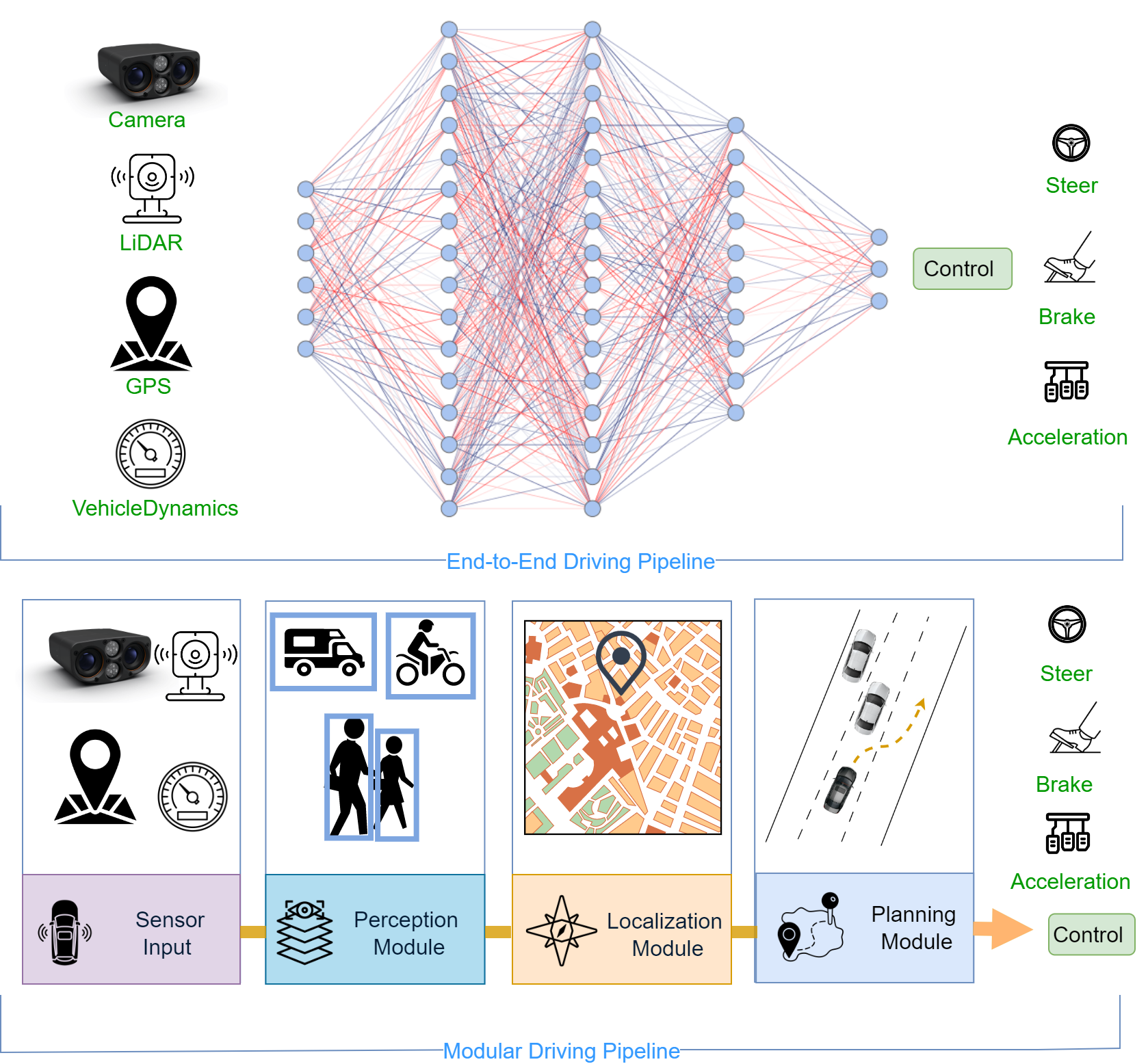
Autonomous driving refers to the capability of a vehicle to drive partly or entirely without human intervention. The modular architecture [1, 2, 3, 4, 5] is a widely used approach in autonomous driving systems, which divides the driving pipeline into discrete sub-tasks. This architecture relies on individual sensors and algorithms to process data and generate control outputs. It encompasses interconnected modules, including perception, planning, and control. However, the modular architecture has certain drawbacks that impede further advancements in autonomous driving (AD). One significant limitation is its susceptibility to error propagation. For instance, errors in the perception module of a self-driving vehicle, such as misclassification, can propagate to subsequent planning and control modules, potentially leading to unsafe behaviors. Additionally, the complexity of managing interconnected modules and the computational inefficiency of processing data at each stage pose additional challenges associated with the modular approach. To address these shortcomings, an alternative approach called End-to-End driving [6, 7, 8, 9, 10, 11] has emerged. This approach aims to overcome the limitations of the modular architecture.

Figure 1: The number of articles in the Web of Science database containing the keywords ‘End-to-End’ and ‘Autonomous Driving’ from 2014 to 2022 illustrates the increasing trend in the research community.

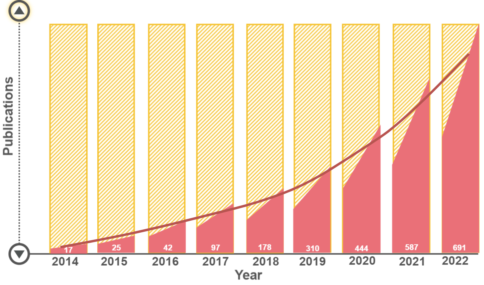
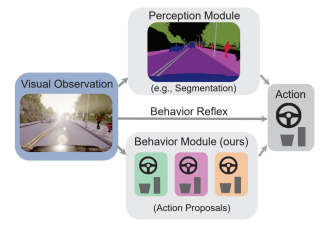
The End-to-End approach streamlines the system, improving efficiency and robustness by directly mapping sensory input to control outputs. The benefits of End-to-End autonomous driving have garnered significant attention in the research community as shown in Fig. 1. Firstly, End-to-End driving addresses the issue of error propagation, as it involves a single learning task pipeline [12, 13] that learns task-specific features, thereby reducing the likelihood of error propagation. Secondly, End-to-End driving offers computational advantages. Modular pipelines often entail redundant computations, as each module is trained for task-specific outputs [4, 5]. This results in unnecessary and prolonged computation. In contrast, End-to-End driving focuses on the specific task of generating the control signal, reducing the need for unnecessary computations and streamlining the overall process. End-to-End models were previously regarded as “black boxes", lacking transparency. However, recent methodologies have improved interpretability in End-to-End models by generating auxiliary outputs [7, 13], attention maps [14, 15, 16, 9, 17, 18], and interpretable maps [18, 19, 8, 20, 12, 21]. This enhanced interpretability provides insights into the root causes of errors and model decision-making. Furthermore, End-to-End driving demonstrates resilience to adversarial attacks. Adversarial attacks [22] involve manipulating sensor inputs to deceive or confuse autonomous driving systems. In End-to-End models, it is challenging to identify and manipulate the specific driving behavior triggers as it is unknown what causes specific driving patterns. Lastly, End-to-End driving offers ease of training. Modular pipelines require separate training and optimization of each task-driven module, necessitating domain-specific knowledge and expertise. In contrast, End-to-End models can learn relevant features and patterns [23, 24] directly from raw sensor data, reducing the need for extensive engineering and expertise.

Figure 2: The charts illustrate statistics of the papers included in this survey according to learning approaches (section 6), environment being utilized for training (sections 10, 11), input modality (section 4), and output modality (section 5).

Related Surveys: A number of related surveys are available, though their emphasis differs from ours. The author Yurtsever et al. [25] covers the autonomous driving domain with a primary emphasis on the modular methodology. Several past surveys center around specific learning techniques, such as imitation learning [26] and reinforcement learning [27]. A few end-to-end surveys, including the work by Tampuu et al. [28], provide an architectural overview of the complete end-to-end driving pipeline. Recently, Chen et al. [29] discuss the methodology and challenges in end-to-end autonomous driving in their survey. Our focus, however, is on the latest advancements, including modalities, learning principles, safety, explainability, and evaluation (see Table LABEL:literature).

Motivation and Contributions: The End-to-End architectures have significantly enhanced autonomous driving systems. As elaborated earlier, these architectures have overcome the limitations of modular approaches. Motivated by these developments, we present a survey on recent advancements in End-to-End autonomous driving. The key contributions of this paper are threefold. First, this survey exclusively explores End-to-End autonomous driving using deep learning. We provide a comprehensive analysis of the underlying principles, methodologies, and functionality, delving into the latest state-of-the-art advancements in this domain. Second, we present a detailed investigation in terms of modality, learning, safety, explainability, and results, and provide a quantitative summary in Table LABEL:literature. Third, we present an evaluation framework based on both open and closed-loop assessments and compile a summarized list of available datasets and simulators.

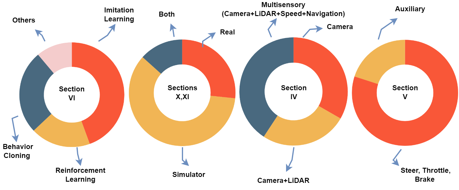
Paper Organization: The survey is organized as per the underlying principles and methodologies (see Fig. 2). We present the background of modular systems in Section 2. Section 3 provides an overview of the End-to-End autonomous driving pipeline architecture. This is followed by sections 4 and 5, which discuss the input and output modalities of the End-to-End system. Section 6 comprehensively covers End-to-End learning methods, from imitation learning to reinforcement learning. The domain adaptation is explained in section 7. Next, we explore the safety aspect of End-to-End approaches in section 8. The importance of explainability and interpretability is discussed in section 9. The evaluation of the End-to-End system consists of open and closed-loop evaluations, which are discussed in section 10. The relevant datasets and the simulator are presented in section 11. Finally, sections 12 and 13 provide the future research direction and conclusion, respectively.

2 Modular system architecture

The modular pipeline [30, 31, 32, 2, 3, 33, 34] begins by inputting the raw sensory data into the perception module for obstacle detection and localization via the localization module, followed by planning and prediction for the optimal and safe trajectory of the vehicle. Finally, the motor controller outputs the control signals. The standard modules of the modular driving pipeline are listed below:

2.1 Components of modular pipeline

Preception:

The perception module seeks to achieve a better understanding [32] of the scene. It is built on top of algorithms such as object detection and lane detection. The perception module is responsible for sensor fusion, information extraction, and acts as a mediator between the low-level sensor input and the high-level decision module. It fuses heterogeneous sensors to capture and generalize the environment. The primary tasks of the perception module include: (i) Object detection (ii) Object tracking (iii) Road and lane detection

Figure 3: The perception module receives and processes various raw sensor inputs, which are then utilized by the localization and mapping module.

Localization and mapping:

Localization is the next important module, which is responsible for determining the position of the ego vehicle and the corresponding road agents [35]. It is crucial for accurately positioning the vehicle and enabling safe maneuvers in diverse traffic scenarios. The end product of the localization module is an accurate map. Some of the localization techniques include High Definition map (HD map) and Simultaneous Localization And Mapping (SLAM), which serve as the online map and localize the traffic agents at different time stamps. The localization mapping can further be utilized for driving policy and control commands.

Planning and driving policy:

The planning and driving policy module [36] is responsible for computing a motion-level command that determines the control signal based on the localization map provided by the previous module. It predicts the optimal future trajectory [37] based on past traffic patterns. The categorization of trajectory prediction techniques (Table 1) is as follows:

• Physics-based methods: These methods are suitable for vehicle motion that can be accurately characterized by kinematics or dynamics models. They can simulate various scenarios quickly with minimal computational cost.

• Classic machine learning-based methods: Compared to physics-based approaches, this class of methods can consider more variables, provide reasonable accuracy, and have a longer forecasting span, but at a higher computing cost. Most of these techniques use historical motion data to estimate future trajectories.

• Deep learning-based methods: Deep learning algorithms are capable of reliable prediction over a wider range of prediction horizons. In contrast, standard trajectory prediction methods are only suited for basic scenes and short-term prediction. Deep learning-based systems can make precise predictions across a wider time horizon. As shown in Table 2, deep learning utilizes RNN, CNN, GNN, and other networks for feature extraction, calculating interaction strength, and incorporating map information.

• Reinforcement learning-based methods: These methods aim to mimic how people make decisions and learn the reward function by studying expert demonstrations to produce the best driving strategy. However, most of these techniques are computationally costly.

Table 1: Performance of different driving policy approaches: PB (Physics-Based), CML (Classical Machine Learning), DL (Deep Learning), RL (Reinforcement Learning).

Techniques	Accuracy	Computation cost	Prediction distance
PB	Medium	Low	Short
CML	Low	Medium	Medium
DL	Highly accurate	High	Wide
RL	Highly accurate	High	Wide

Table 2: Summary of deep learning-based approaches for motion prediction utilizing different backbone networks.

Methods	Detail	Classification	Agent and context encoder	Context encoder	Decoder
CoverNet [38]	Formulation of classification problem over the set of diverse trajectories	CNN	CNN	CNN	Trajectory set generator
HOME [39]	It outputs the 2D top view representation of agent possible future	CNN	CNN,GRU	CNN	CNN
TPCN [40]	Splitting of trajectory prediction into both temporal and spatial dimension	CNN	PointNET ++	PointNET++	Displacement prediction
MHA-JAM [41]	Attention head is used to generate distinct future trajectories while addressing multimodality	Attention	LSTM	CNN	LSTM
MMTransformer [42]	Network architecture based on stacked transformer to model the feature multimodality	Attention	Transformer	VectorNet	MLP
DenseTNT [43]	It is a anchor-free model which directly outputs from the dense goal candidates	GNN	VectorNet	VectorNet	Goal Bases multi-trajectory prediction
TS-GAN [44]	Collaborative learning and GAN for modeling motion behavior	Generative model	LSTM	-	LSTM
PRIME [44]	Utilizes the model generator and learning based evaluator	Generative model	CNN,LSTM	LSTM	Model-based generator
MotionDiff [45]	Diffusion probability based kinematics model to diffuse original states to noise distribution	CNN	Spatial transformer, GRU	Spatial transformer, GRU	MLP
ScePT [10]	A policy planning based trajectory prediction for accurate motion planning.	GNN	LSTM	CNN	GRU, PonitNET

Control:

The motion planner generates the trajectory, which is then updated by the obstacle subsystem and sent to the controller subsystem. The computed command is sent to the actuators of the driving components, including the throttle, brakes, and steering, to follow the desired trajectory, which is optimized and safer in real-world scenarios. The Proportional Integral Derivative (PID) [5] and Model Predictive Control (MPC) [4] are some of the controllers used to generate the aforementioned control signals.

2.2 Input and output modality of modular pipeline

The output modality of each module is designed to be compatible with the input modality of subsequent modules in the pipeline to ensure that information is correctly propagated through the modular system.

Sensory data:

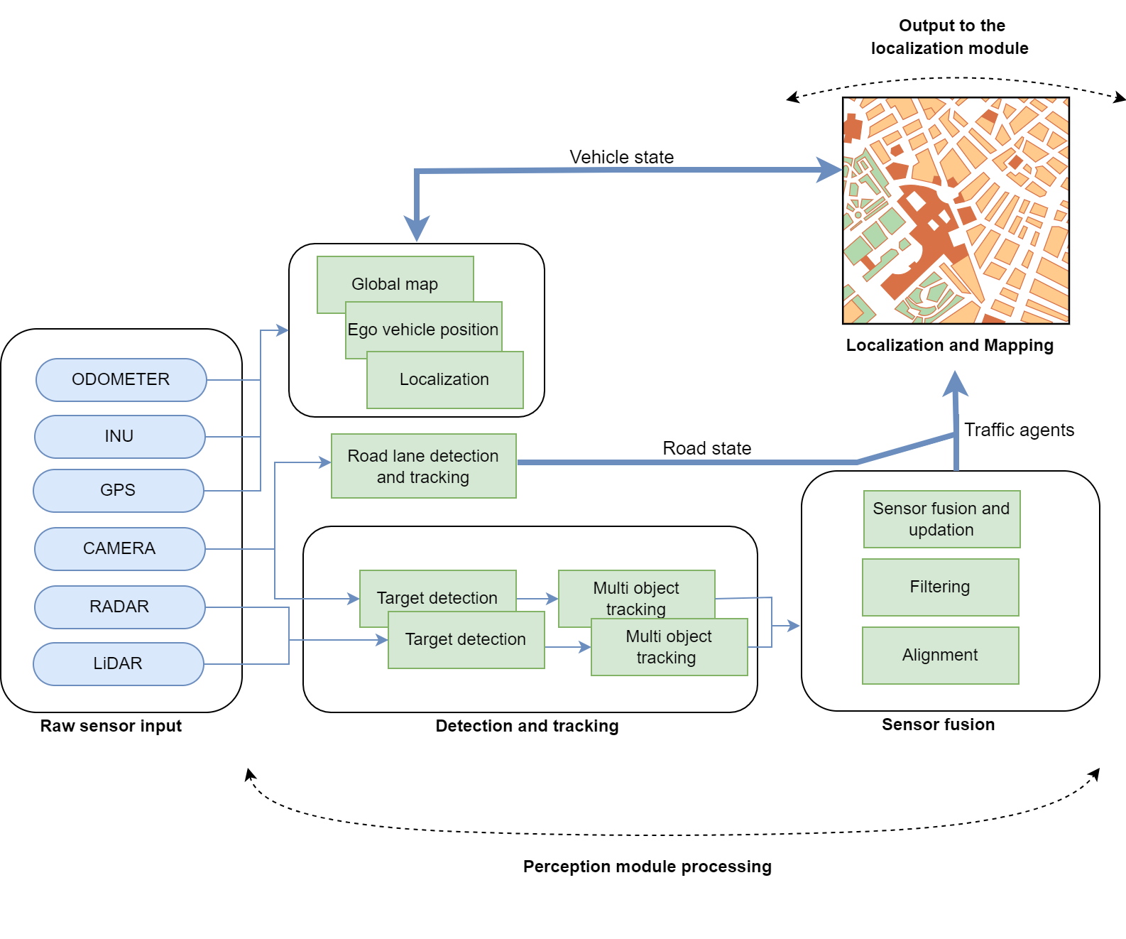
At this level (Fig. 3), the raw data from the embedded multi-sensor array is retrieved, filtered, and processed for semantic mapping. LiDAR, RADAR, Camera, GPS, and Odometer are some of the sensor inputs to the perception stack. LiDAR and RADAR are used for depth analysis, while cameras are employed for detection. The INU, GPS, and Odometer sensors capture and map the vehicle’s position, state, and the corresponding environment, which can be further utilized by decision-level stages.

Input to the mapping and localization:

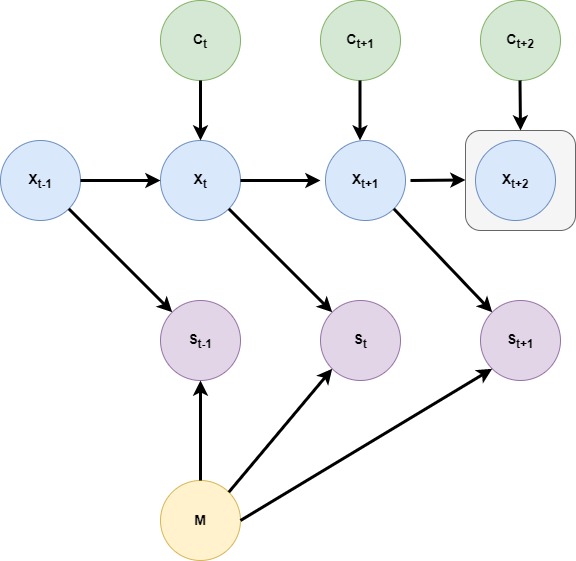
Localization aims to estimate the vehicle’s position at each time stamp. Utilizing information from the perception module, the vehicle’s position and the environment are mapped based on parameters such as position, orientation, pose, speed, and acceleration. Localization techniques [3] allow for the integration of multiple objects and the identification of their relationships, resulting in a more comprehensive, augmented, and enriched representation.

As shown in Fig. 4, we define $X_{t}$ as the vehicle’s position estimate at time $t$, and $M$ as the environment map. These variables can be estimated using control inputs $C_{t}$, which are typically derived from wheel encoders or sensors capable of estimating the vehicle’s displacement. The measurements derived from sensor readings are denoted by $S_{t}$ and are used to aid in the estimation of the vehicle’s pose.

Figure 4: Visualization of temporal correlations from localization that can be used to identify specific behaviors and predict future positions.

Input to the path planning and decision module:

Path planning is broadly categorized into local and global path planners. The purpose of the local planner is to execute the goals set by the global path planner. It is responsible for finding trajectories that avoid obstacles and satisfy optimization requirements within the vehicle’s operational space.

The problem of local trajectory prediction can be formulated as estimating the future states ($t_{f}$) of various traffic actors ($R^{t}$) in a given scenario based on their current and past states ($t_{h}$). The state of traffic actors includes vehicles or pedestrians with historical trajectories at different time stamps.

$$Input=\{R^{1},R^{2},R^{3},R^{3}.\;.\;.\;.\;.\;.,R^{t_{h}}\}$$ (1)

where $R^{t}$ contains the coordinates of different traffic actors at each time stamp $t$ (up to $h$ past time stamps).

$$R^{t}=\{x_{0}^{t},y_{0}^{t},x_{1}^{t},y_{1}^{t}\;.\;.\;.\;x_{n}^{t},y_{n}^{t}\}$$ (2)

where $n$ represents all traffic vehicles detected by the ego vehicle; ($x_{i}^{t},y_{i}^{t}$) are the coordinates of the vehicle at the $t$ time stamp. $X$ is the input to the path planning module, and the vehicle trajectory $Y$ is predicted from the model at future time stamp $t_{f}$.

$$Y=\left\{R^{t_{h}+1},R^{t_{h}+2},R^{t_{h}+3}\cdot\cdot\cdot R^{t_{h}+t_{f}}\right\}$$ (3)

Input to the control module:

There are two primary forms of trajectory command that the controller receives: (i) as a series of commands ($T_{c}$) and (ii) as a series of states ($T_{s}$). Controller subsystems that receive a $T_{s}$ trajectory may be categorized as path tracking techniques, while those that receive a $T_{c}$ trajectory can be classified as direct hardware actuation control methods.

• Direct hardware actuation control methods: The Proportional Integral Derivative (PID) [5] control system is a commonly used hardware actuation technique for self-driving automobiles. It involves determining a desired hardware input and an error measure gauging how much the output deviates from the desired outcome.

• Path tracking methods: Model Predictive Control (MPC) [4] is a path-tracking approach that involves choosing control command inputs that will result in desirable hardware outputs, then simulating and optimizing those outputs using the motion model of the car over a future prediction horizon.

3 End-to-End system architecture

In general, modular systems are referred to as the mediated paradigm and are constructed as a pipeline of discrete components (Fig. 5) that connect sensory inputs and motor outputs. The core processes of a modular system include perception, localization, mapping, planning, and vehicle control [1]. The modular pipeline starts by inputting raw sensory data to the perception module for obstacle detection [46] and localization via the localization module [3]. This is followed by planning and prediction [44] to determine the optimal and safe trajectory for the vehicle. Finally, the motor controller generates commands for safe maneuvering.

On the other hand, direct perception or End-to-End driving directly generates ego-motion from the sensory input. It optimizes the driving pipeline (Fig. 5) by bypassing the sub-tasks related to perception and planning, allowing for continuous learning to sense and act, similar to humans. The first attempt at End-to-End driving was made by Pomerleau Alvinn [47], which trained a 3-layer sensorimotor fully connected network to output the car’s direction. End-to-End driving generates ego-motion based on sensory input, which can be of various modalities. However, the prominent ones are the camera [48, 49, 50], Light Detection and Ranging (LiDAR) [6, 10, 7], navigation commands [51, 49, 23], and vehicle dynamics, such as speed [52, 53, 50]. This sensory information is utilized as the input to the backbone model, which is responsible for generating control signals. Ego-motion can involve different types of motions, such as acceleration, turning, steering, and pedaling. Additionally, many models also output additional information, such as a cost map for safe maneuvers, interpretable outputs, and other auxiliary outputs.

Figure 5: Comparison between End-to-End and modular pipelines. End-to-End is a single pipeline that generates the control signal directly from perception input, whereas a modular pipeline consists of various sub-modules, each with task-specific functionalities.

There are two main approaches for End-to-End driving: either the driving model is explored and improved via Reinforcement Learning (RL) [54, 53, 55, 56, 21, 57], or it is trained in a supervised manner using Imitation Learning (IL) [18, 6, 19, 15, 17, 58, 7] to resemble human driving behavior. The supervised learning paradigm aims to learn the driving style from expert demonstrations, which serve as training examples for the model. However, expanding an autonomous driving system based on IL [23] is challenging since it is impossible to cover every instance during the learning phase. On the other hand, RL works by maximizing cumulative rewards [59, 55] over time through interaction with the environment, and the network makes driving decisions to obtain rewards or penalties based on its actions. While RL model training occurs online and allows exploration of the environment during training, it is less effective in utilizing data compared to imitation learning. Table LABEL:literature summarizes recent methods in End-to-End driving.

4 Input modalities in End-to-End system

The following section explores the input modalities essential for end-to-end autonomous driving. These encompass cameras for visual insights, LiDAR for precise 3D point clouds, multi-modal inputs, and navigational inputs. Fig. 6 illustrates some of the input and output modalities.

4.1 Camera

Camera-based methods [14, 9, 6, 23, 49, 60, 50, 53, 12, 13] have shown promising results in End-to-End driving. For instance, Toromanoff et al. [53] demonstrated their capabilities by winning the CARLA 2019 autonomous driving challenge using vision-based approaches in an urban context. The use of monocular [13, 11, 61, 53] and stereo vision [58, 17, 15] camera views is a natural input modality for image-to-control End-to-End driving. Xiao et al. [62] employed inputs consisting of a monocular RGB image from a forward-facing camera and the vehicle speed. Chen et al. LAV [10] utilize only the camera image input as shown in Fig. 6(d). Wu et al. [15], Xiao et al. [17], Zhang et al. [58] utilize camera-only modality to generate high-level instructions for lane following, turning, stopping and going straight using imitation learning.

4.2 LiDAR

Another significant input source in self-driving is the Light Detection and Ranging (LiDAR) sensor. LiDAR [63, 64, 65, 20] is resistant to lighting conditions and offers accurate distance estimates. Compared to other perception sensors, LiDAR data is the richest and provides the most comprehensive spatial information. It utilizes laser light to detect distances and generates PointClouds, which are 3D representations of space where each point includes the $(x,y,z)$ coordinates of the surface that reflected the sensor’s laser beam. When localizing a vehicle, generating odometry measurements is critical. Many techniques utilize LiDAR for feature mapping in Birds Eye View (BEV) [9, 19, 16], High Definition (HD) map [20, 66], and Simultaneous Localization and Mapping (SLAM) [67]. Shenoi et al. [68] have shown that adding depth and semantics via LiDAR has the potential to enhance driving performance. Liang et al. [69, 70] utilized point flow to learn the driving policy in an End-to-End manner.

4.3 Multi-modal

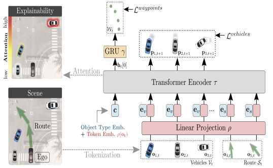
Multimodality [8, 18, 10, 16, 71] outperforms single modality in crucial perception tasks and is particularly well-suited for autonomous driving applications, as it combines multi-sensor data. There are three broad categorizations for utilizing information depending on when to combine multi-sensor information. In early fusion, sensor data is combined before feeding them into the learnable End-to-End system. Chen et al. [10] as shown in Fig. 6(d) use a network that accepts (RGB + Depth) channel inputs, Xiao et al. [62] model also input the same modality. The network modifies just the first convolutional layer to account for the additional input channel, while the remaining network remains unchanged. Renz et al. [18] fuse object-level input representation using a transformer encoder. The author combinedly represents a set of objects as vehicles and segments of the routes.

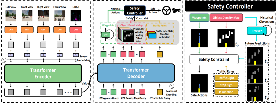
In mid-fusion, information fusion is done either after some preprocessing stages or after some feature extraction. Zhou et al. [72] perform information fusion at the mid-level by leveraging the complementary information provided by both the bird’s-eye view (BEV) and perspective views of the LiDAR point cloud. Transfuser [7] as shown in Fig. 6(a) addresses the integration of image and LiDAR modalities using self-attention layers. They utilized multiple transformer modules at multiple resolutions to fuse intermediate features. Obtained feature vector forms a concise representation which an MLP then processes before passing to an auto-regressive waypoint prediction network. In late fusion, inputs are processed separately, and their output is fused and further processed by another layer. Some authors [73, 69, 70, 62] use a late fusion architecture for LiDAR and visual modalities, in which each input stream is encoded separately and concatenated.

4.4 Navigational inputs

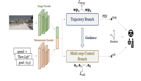
End-to-End navigation input can originate from the route planner [8, 14, 74] and navigation commands [48, 75, 76, 77]. Routes are defined by a sequence of discrete endpoint locations in Global Positioning System (GPS) coordinates provided by a global planner [14]. The TCP model [13] as illustrated in Fig. 6(c) is provided with correlated navigation directives like lane keeping, left/right turns, and the destination. This information is used to produce the control actions.

Shao et al. [8] propose a technique that guides driving using these sparse destination locations instead of explicitly defining discrete navigation directives. PlanT [18] utilizes point-to-point navigation based on the input of the goal location. FlowDriveNet [78] considers both the global planner’s discrete navigation command and the coordinates of the navigation target. Hubschneider et al. [75] include a turn indicator command in the driving model, while Codevilla et al. [76] utilize a CNN block for specific navigation tasks and a second block for subset navigation. In addition to the aforementioned inputs, End-to-End models also incorporate vehicle dynamics, such as ego-vehicle speed [52, 49, 53, 12].

5 Output modalities in End-to-End system

Usually, an End-to-End autonomous driving system outputs control commands, waypoints, or trajectories. In addition, it may also produce additional representations, such as a cost map and auxiliary outputs.

5.1 Waypoints

Predicting future waypoints is a higher-level output modality. Several authors [10, 6, 7, 79] use an auto-regressive waypoint network to predict differential waypoints. Trajectories [8, 74, 80, 13, 19] can also represent sequences of waypoints in the coordinate frame. The network’s output waypoints are converted into low-level steering and acceleration using Model Predictive Control (MPC) [4] and Proportional Integral Derivative (PID) [5]. The longitudinal controller considers the magnitude of a weighted average of vectors between successive time-step waypoints, while the lateral controller considers their direction. The ideal waypoint [53] relies on desired speed, position, and rotation.

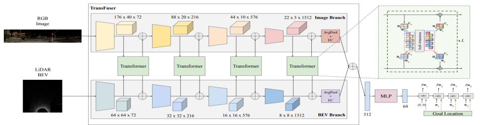(a) Fusion Transformer

b) NEAT

(c) TCP

(d) LAV

(e) UniAD

(f) ST-P3

Figure 6: The input-output representation of various End-to-End models: (a) Considered RGB image and LiDAR BEV representations as inputs to the multi-modal fusion transformer [7] and predicts the differential ego-vehicle waypoints. (b) NEAT [12] inputs the image patch and velocity features to obtain a waypoint for each time-step used by PID controllers for driving. (c) TCP [13] takes input image i, navigation information g, current speed v, to generate the control actions guided by the trajectory branch and control branch. (d) LAV [10] uses an image-only input and predicts multi-modal future trajectories used for braking and handling traffic signs and obstacles. (e) UniAD [9] generates attention mask visualization which shows how much attention is paid to the goal lane as well as the critical agents that are yielding to the ego-vehicle.(f) ST-P3 [20] outputs the sub cost map from the prediction module (darker color indicates a smaller cost value). By incorporating the occupancy probability field and leveraging pre-existing knowledge, the cost function effectively balances safety considerations for the final trajectory.

The lateral distance and angle must be minimized to maximize the reward (or minimize the deviation). The benefit of utilizing waypoints as an output is that they are not affected by vehicle geometry. Additionally, waypoints are easier to analyze by the controller for control commands such as steering. Waypoints in continuous form can be transformed into a specific trajectory. Zhang et al. [54] and Zhou et al. [74] utilize a motion planner to generate a series of waypoints that describe the future trajectory. LAV [10] predicts multi-modal future trajectories (Fig. 6(d)) for all detected vehicles, including the ego-vehicle. They use future waypoints to represent the motion plan.

5.2 Cost function

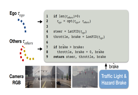
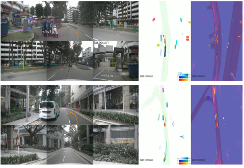
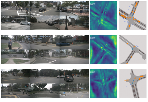
Many trajectories and waypoints are possible for the safe maneuvering of the vehicle. The cost [20, 81, 56, 21, 80, 82] is used to select the optimal one among the possibilities. It assigns a weight (positive or negative score) to each trajectory based on parameters defined by the end user, such as safety, distance traveled, comfort, and others. Rhinehart et al. [83] and Chen et al. [10] refine control using the predictive consistency map, which updates knowledge at test time. They also evaluate the trajectory using an ensemble expert likelihood model. Prakash et al. [14] utilize object-level representations to analyze collision-free routes. Zeng et al. [84] employ a neural motion planner that uses a cost volume to predict future trajectories. Hu et al. [20] employ a cost function illustrated in Fig. 6(f) that takes advantage of the learned occupancy probability field, represented by segmentation maps, and prior knowledge such as traffic rules to select the trajectory with the minimum cost. Regarding safety cost functions, Zhao et al. [50], Chen et al. [85], and Shao et al. [8] employ safety maps. They analyze actions within the safe set to create causal insights regarding hazardous driving situations.

Figure 7: Vehicle maneuvers, represented by a triplet of steering angle, throttle, and brake, depend on a high-level route navigation command (e.g., turn-left, turn-right, go-straight, continue), as well as perception data (e.g., RGB image) and vehicle state measurements (e.g., speed). These inputs guide the specific actions taken by the vehicle, enabling it to navigate the environment effectively through conditional imitation learning [62].

5.3 Direct control and acceleration

Most of the End-to-End models [83, 74, 53, 48, 23, 75, 76, 77, 48] provide the steering angle and speed as outputs at a specific timestamp. The output control needs to be calibrated based on the vehicle’s dynamics, determining the appropriate steering angle for turning and the necessary braking for stopping at a measurable distance.

5.4 Auxiliary output

The auxiliary output can provide additional information for the model’s operation and the determination of driving actions. Several types of auxiliary outputs include the segmentation map [9, 7] (Fig. 6(e)), BEV map [12, 9, 19, 16], future occupancy [18, 9, 84, 82] of the vehicle (Fig. 6(e)), and interpretable feature map [18, 8, 7, 20, 12, 81] (Fig. 6(b)(f)). These outputs provide additional functionality to the End-to-End pipeline and help the model learn better representations. The auxiliary output also facilitates the explanation of the model’s behavior [7, 82], as one can comprehend the information and infer the reasons behind the model’s decisions.

6 Learning approaches for End-to-End system

The following sections discuss various learning approaches in End-to-End Driving, including imitation learning and reinforcement learning.

6.1 Imitation learning

Imitation learning (IL) [10, 18, 13, 14, 86] is based on the principle of learning from expert demonstrations. These demonstrations train the system to mimic the expert’s behavior in various driving scenarios. Large-scale expert driving datasets are readily available, which can be leveraged by imitation learning [62] to train models that perform at human-like standards.

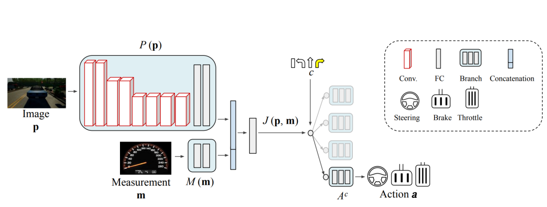
The main objective is to train a policy $\pi_{\theta}(s)$ that maps each given state to a corresponding action (Fig. 7) as closely as possible to the given expert policy $\pi^{*}$, given an expert dataset with state action pair $\left(s,a\right)$:

$$\arg\min_{\theta}E_{s}\sim_{P(s\mid\theta)}L(\pi^{*}(s),\pi_{\theta}(s))$$ (4)

where $P(s\mid\theta)$ represents the state distribution of the trained policy $\pi_{\theta}$.

Behavioural Cloning (BC), Direct Policy Learning (DPL), and Inverse Reinforcement Learning (IRL) are extensions of imitation learning in the domain of autonomous driving.

6.1.1 Behavioural cloning

Behavioural cloning [87, 7, 13, 12, 49, 23, 88] is the supervised imitation learning task where the goal is to treat each state-action combination in expert distribution as an Independent and Identically Distributed (I.I.D) example and minimise imitation loss for the trained policy:

$$\arg\min_{\theta}E_{(s,a^{*})}\sim_{P^{*}}L(a^{*},\pi_{\theta}(s))$$ (5)

where $p^{*}(s\mid\pi^{*})$ is an expert policy state distribution, and (state s, action $a^{*}$) is provided by expert policy $p^{*}$.

Figure 8: Behavior cloning [49] is a perception-to-action driving model that learns behavior reflex for various driving scenarios. The agent acquires the ability to integrate expert policies in a context-dependent and task-optimized manner, allowing it to drive confidently.

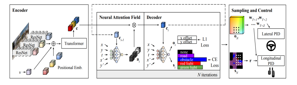
Prakash et al. [14], Chitta et al. [7], NEAT [12], Ohn et al. [49] utilize a policy that maps input frames to low-level control signals in terms of waypoints. These waypoints are then fed into a PID to obtain the steering, throttle, and brake commands based on the predicted waypoints. Behavior cloning [49] assumes that the expert’s actions can be fully explained by observation, as it trains a model to directly map from input to output based on the training dataset (Fig. 8). However, this leads to the distribution shift problem, where the actual observations diverge from the training observations. Many latent variables impact and govern driving agent’s actions in real-world scenarios. Therefore, it is essential to learn these variables effectively.

6.1.2 Direct policy learning

Within the context of BC, which maps sensor inputs to control commands and is limited by the training dataset, DLP aims to learn an optimal policy [48] directly that maps inputs to driving actions. The DLP algorithm obtains expert evaluations [56] during runtime to gather more training data, particularly for scenarios where the initial policy falls short. It combines an expert dataset with Imitation Learning for initial training and iteratively augments the dataset with additional trajectories collected by the trained policy. The agent can explore its surroundings and discover novel and efficient driving policies.

The online imitation learning algorithm DAGGER [89] provides robustness against cascading errors and accumulates additional training instances. Chen et al. [10] introduced automated dagger-like monitoring, where the privileged agent’s supervision is collected through online learning and transformed into an agent that provides on-policy supervision. However, the main drawback of direct policy learning is the continuous need for expert access during the training process, which is both costly and inefficient.

6.1.3 Inverse reinforcement learning

Inverse Reinforcement Learning (IRL) [90, 48] aims to deduce the underlying specific behaviours through the reward function. Expert demonstrations $D=\left\{\zeta_{1},\zeta_{2},\zeta_{3},......,\zeta_{n}\right\}$ are fed into IRL. Each $\zeta_{i}=\left\{(s_{1},a_{2}),(s_{2},a_{2}),.....(s_{n},a_{n})\right\}$ consists of a state-action pair. The principal goal is to get the underlying reward which can be used to replicate the expert behaviour. Feature-based IRL [91] teaches the different driving styles in the highway scenario. The human-provided examples are used to learn different reward functions and capabilities of interaction with road users. Maximum Entropy (MaxEnt) inverse reinforcement learning [92] is an extension of the feature-based IRL based on the principle of maximum entropy. This paradigm robustly addresses reward ambiguity and handles sub-optimization. The major drawback is that IRL algorithms are expensive to run. They are also computationally demanding, unstable during training, and may take longer to converge on smaller datasets.

(a) Roach Expert Supervision

(b) Human Copilot Learning

Figure 9: RL-based learning method for training the agent to drive optimally: (a) Illustrating the reinforcement learning expert [54] that maps the BEV to the low-level driving actions; the expert can also provide supervision to the imitation learning agent. (b) Human-in-the-loop learning [55] allows the agent to explore the environment, and in danger scenarios, the human expert takes over the control and provides the safe demonstration.

6.2 Reinforcement learning

Reinforcement Learning (RL) [93, 57, 56, 53] is a promising approach to address the distribution shift problem. It aims to maximize cumulative rewards [94] over time by interacting with the environment, and the network makes driving decisions to obtain rewards or penalties based on its actions. IL cannot handle novel situations significantly different from the training dataset, RL is robust to this issue as it explores scenario under given environment. Reinforcement learning encompasses various models, including value-based models such as Deep Q-Networks (DQN) [95], actor-critic based models like Deep Deterministic Policy Gradient (DDPG) and Asynchronous Advantage Actor Critic (A3C) [95], maximum entropy models [92] such as Soft Actor Critic (SAC) [96], and policy-based optimization methods such as Trust Region Policy Optimization (TRPO) and Proximal Policy Optimization (PPO) [97].

Liang et al. [98] demonstrated the first effective RL approach for vision-based driving pipelines that outperformed the modular pipeline at the time. Their method is based on the Deep Deterministic Policy Gradient (DDPG), an extended version of the actor-critic algorithm. Chen et al. [99] uses tabular-RL to first learn an expert policy and then uses policy distillation to learn a student policy in an imitation learning approach.

Recently, Human-In-The-Loop (HITL) approaches [100, 55, 56, 54, 14] have gained attention in the literature. These approaches are based on the premise that expert demonstrations provide valuable guidance for achieving high-reward policies. Several studies have focused on incorporating human expertise into the training process of traditional RL or IL paradigms. One such example is EGPO [56], which aims to develop an expert-guided policy optimization technique where an expert policy supervises the learning agent.

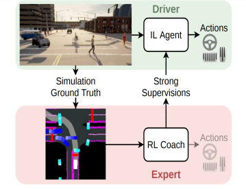
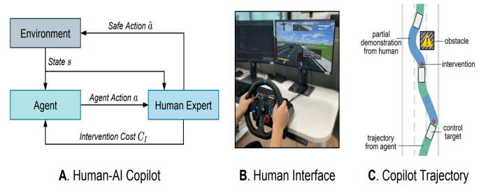
HACO [55] allows the agent to explore hazardous environments while ensuring training safety. In this approach, a human expert can intervene and guide the agent to avoid potentially harmful situations or irrelevant actions (see Fig. 9(b)). Another reinforcement learning expert, Roach [54], translates bird’s-eye view images into continuous low-level actions (see Fig. 9(a)). Experts can provide high-level supervision for imitation learning or reinforcement learning in general. Policies can be initially taught using imitation learning and then refined using reinforcement learning, which helps reduce the extensive training period required for RL. Jia et al. [19] utilize features extracted from Roach to learn the ground-truth action/trajectory, providing supervision in their study. Therefore, reinforcement learning provides a solution to address the challenges of imitation learning by enabling agents to actively explore and learn from their environment. There are also associated challenges, such as sample inefficiency, exploration difficulties leading to suboptimal behaviors, and difficulties generalizing learned policies to new scenarios.

7 Learning domain adaptation from simulator to real

Large-scale virtual scenarios can be constructed in virtual engines, enabling the collection of a significant quantity of data more readily. However, there still exist significant domain disparities between virtual and real-world data, which pose challenges in creating and implementing virtual datasets. By leveraging the principle of domain adaptation, we can extract critical features directly from the simulator and transfer the knowledge learned from the source domain to the target domain, consisting of accurate real-world data.

The H-Divergence framework [101] resolves the domain gap at both the visual and instance levels by adversarially learning a domain classifier and a detector simultaneously. Zhang et al. [102] propose a simulator-real interaction strategy that leverages disparities between the source domain and the target domain. The authors create two components to align differences at the global and local levels and ensure overall consistency between them. The realistic-looking synthetic images may subsequently be used to train an End-to-End model. A number of techniques rely on an open pipeline that introduces obstacles in the current environment. PlaceNet [103] places objects into the image space for detection and segmentation operations. GeoSim [104] is a geometry-aware approach that dynamically inserts objects using LiDAR and HD maps. DummyNet [105] is a pedestrian augmentation framework based on a GAN architecture that takes the background image as input and inserts pedestrians with consistent alignment. Some works take advantage of virtual LiDAR data [106, 107, 108]. Sallab et al. [106] perform learning on virtual LiDAR point clouds from CARLA [109] and utilize CycleGAN to transfer styles from the virtual domain to the real KITTI [110] dataset. Fang et al. [107] propose a LiDAR simulator that

Table 3: RECENT METHODS IN END-TO-END AUTONOMOUS DRIVING

Paper, Year	Environment	Input modality	Output modality	Learning	Evaluation	Explaibility	Safety	Results	Data
PAD [9], 2023	NuScenes	6 Multi-camera images	Segmentation map, agent future trajectories, future occupancy	Multi-task learning.	min ADE, min FDE, IoU, L2 error	Exp. Via attention mask in planner module	Lowest collision rate, lowest L2 error, Safety boost via goal planner.	L2: 1.65 CR: 0.71	Perception training: 6 epochs Joint training: 20 epochs
ReasonNet [16], 2023	CARLA	Vehicle measurements navigation, LiDAR, RGB	Steering, speed, BEV, brake	Multi-task learning	DOS and LeaderBoard	Attention map	-	DS: 79.95 RC: 89.89 IS: 0.89	Train: 2M frames (eight Towns) Test: Town05
Policy Pre-Training [111], 2023	NuScenes, CARLA	Camera and intrinsics	Steering, throttle	Imitation learning	Longest6, collision rate	Attention activation map	Handles cases where the agent needs to stop	DS: 47.4$\pm$5.6 RC: 65.05$\pm$5.1 IS: 0.79$\pm$0.08 L2: 3.01, CR: 0.94	Train: 40K (Town01, 03, 04, 06) Test: 50 routes
Think Twice [19], 2023	CARLA	RGB camera, LiDAR	BEV feature map, agent future trajectories, control actions	Open-loop imitation learning	Longest6	Explainable via expert BEV feature map	Safety-critical regions, anticipate future motion to avoid collisions	DS: 70.9$\pm$3.4 RC: 95.5$\pm$2.6 IS: 0.75$\pm$0.05	Training: 189K data on four Towns, Roach based teaching
Scaling Vision-based [17], 2023	CARLA	Three cameras (views)	Ego-vehicle’s steering angle and acceleration	Self-supervised imitation learning	NoCrash, Leaderboard	Attention map	Pedestrians caused strong braking (0.794), despite green light	DS: 98$\pm$1.7 RC: 68$\pm$2.7	Train: 15 hours (540K frames) Test: 25 hours ( 900k frames)
Coaching a Teachable [58], 2023	CARLA	Navigation, 3 RGB cameras	Waypoints, control commands	Knowledge distillation, imitation learning	Longest6, ADE, FDE	-	Attend to safety-critical entities	DS: 73.30$\pm$1.07 RC: 87.44$\pm$0.28 ADE: 0.41 FDE: 0.36	Train: Town01 - Town06
Hidden Biases of [71], 2023	CARLA	Speed, camera and LiDAR	Steer, throttle, and brake, waypoints, path	Imitation learning	Longest6	-	Larger safety distance, safety area	DS: 72 $\pm$3 RC: 95 $\pm$ 2	Train: variable size 185k and 555k
KING [6], 2022	CARLA	Front-facing camera and LiDAR	Throttle and steering	Behaviour cloning	Closed-loop (CR), (RC), (IS), (DS)	-	Safety-critical driving scenarios and stress-testing.	DS: 90.20$\pm$0.00 RC: 94.42$\pm$0.36 IS: 0.96$\pm$0.36	Train: 4 GPU hours 80 routes on Town 3,4,5,6.
LAV [10], 2022	CARLA	Front-facing camera, LiDAR	Single steering and acceleration command	Knowledge distillation, imitation learning	Longest6 (DS), (RC),(IS), (CR), (PC), (LC), (RV)	Spatial feature 2D map	Scenario such as pedestrians crossing, lane change are modeled	DS: 61.85 RC: 94.46 IS: 0.64	Train: Four Towns, 186K frames Test: Town02 and Town05
TransFuse [7], 2022	CARLA	RGB, LiDAR	Waypoints, steer, throttle, and brake	Behaviour cloning	Longest 6 (DS), (RC), (IPK), (IS)	Explainable via auxiliary output like depth, semantic, HD map, planner A*	Global safety heuristic	DS: 61.18 RC: 86.69 IS: 0.71	Train: 2500 routes on eight Towns, 228k frames Test: 36 route
Learning to Drive [11], 2022	NuScenes, youtube	Front-facing camera	Steering, throttle, brake, and velocity	Conditional behavior cloning	CARLA benchmark, F1 metric	-	-	F1 : 75.0 7 perc. increase in RC	Train: 120 hour YouTube, Test: Town01 and Town02 with 40K transition
HACO [55], 2022	CARLA	Current state, navigation information	Acceleration, brake and steering	Reinforcement learning	Safety violation data usage, success rate	-	Safety violation cost the episode	SV: 11.84 SR: 0.35	Train: 50 min HACO training. 35k transition
PlanT [18], 2022	CARLA	Camera , LiDAR, route, object	Waypoints, predicting the future attributes of other vehicles	Imitation learning	Longest6 CARLA (DS),(RC), (IS), (IPK), (IT)	Post hoc explanations, attention weights for identify relevant objects.	Identification of collision free routes, RFDS algorithm for collision avoidance	DS: 81.36$\pm$6.54 RC: 93.55$\pm$2.62 IS: 0.87$\pm$0.05	Train: 3.2 hours on PlanT, 95 hours of driving.
Trajectory-guided [13], 2022	CARLA	Monocular camera	Steering, throttle and brake	Behaviour cloning	CARLA (DS), (RC), (IS)	Auxiliary tasks include value and speed head	Reduce collision via long prediction, less infraction, control model preform good	DS: 75.14 RC: 85.63 IS: 0.87	Train: Town01, 03, 04, 06 Test: Town02, 05
Safety- Enhanced Autonomous Driving [8], 2022	CARLA	3 RGB, 1 LiDAR	10 Waypoints, steering, acceleration	InterFuser	CARLA leaderboard, CARLA 42 Routes benchmark, (RC),(IS),(DS)	Intermediate interpretable features output from transformer decoder (safety map, object density)	Safe set contain only safe actions, safety sensitive output via InterFuser	DS: 76.18 RC: 88.23 IS: 0.84	Train: 3M frames or 410 hours (eight Towns)
ST-P3 [20], 2022	NuScenes, CARLA	6 Camera(NuScenes), 4 cameras (CARLA), navigation command	Steering, throttle and brake	ST-P3	Open loop: IOU, PQ, RQ, SQ, L2 error Closed: (DS), (RC)	Interpretable map lanes and area which is drivable	Safety Cost function for the jerk action penalize	DS: 55.14 RC: 86.74 L2: 2.90, CR: 1.27	Train: 26124 samples Validation: 5719 samples
Safe Driving via Expert Guided Policy optimization [56], 2022	MetaDrive	Camera	Control signal	Expert-in-the-loop reinforcement learning	MetaDriv benchmark	-	Guardian to ensure training safety	ER: 388.37 $\pm$10.01 EC: 0.56 $\pm$0.35 SR: 0.85 $\pm$0.05	Train: 100 scenes Test: 50 scenes
COOPERNAUT [88] , 2022	CARLA	Front-facing camera, LiDAR	Control signal	Behaviour cloning	AUTOCASTSIM	-	Reduces safety hazards for line-of sight sensing.	SR: 90.5$\pm$1.2 CR: 4.5$\pm$3.1	Train: 12 traces + 84 traces Test : 27 accident prone traces
Human-AI Shared Control via Policy [21], 2022	MetaDrive	Current state, goal state	Control signal	Reinforcement learning	MetaDrive and Pybullet-A1	Interpretable control interface	Human-AI, safety guarantee 95 percentage success rate	EC: 0.05 $\pm$0.08 SR: 0.95 $\pm$ 0.02	Train: 50 training scenario Test: 20 test scene
MMFN: Multi-Modal Fusion-Net for [66], 2022	CARLA	HD map and radar on top of the LiDAR and camera	Steering, throttle and brake	Imitation learning	CARLA LeaderBoard	-	Expert has more awareness of safe driving	DS: 22.8 RC: 47.22	Train: 207K frames Test: 20 routes
CADRE: A Cascade Deep Reinforcement [57], 2022	CARLA	Front-view camera, position, orientation and speed	Control signal	Imitation learning	CARLA NoCrash	-	-	VA: 81/81 PA: 76/78	Train:25 training routes Test: Town02
Model-Based Imitation Learning for [112], 2022	CARLA	RGB image, route	Vehicle control, BEV Segmentation	Model-based imitation learning	CARLA LeaderBoard	BEV semantic segmentation for interpretability	-	DS: 61.1 $\pm$ 3.2 RC: 97.4$\pm$ 0.8 IS: 63.0 $\pm$ 3.0	Test: Town05, routes Train: Four different training towns total of 2.9M frames.
LookOut: Diverse Multi-Future Prediction and Planning [80], 2021	ATG4D, Lidarsim	LiDAR, navigation.	Trajectory, vehicle control	Cost learning	Open loop: mAP, mSADE, mSADE, PlanASD Cloose loop: Lidarsim	-	Cost function include driving including safety, comfort, traffic-rules.	CR: 7.93 Progress:62.65 Jerk: 4.69	Train: one million frames Test: Lidarsim
MP3: A Unified Model to Map, Perceive, Predict and Plan [82], 2021	URBANEXPERT	Raw sensor data and a high-level command	Control command, dynamic occupancy field	MP3	Closed-loop: Lidarsim Open loop: L2	Interpretable cost functions, dynamic occupancy field, Interpretable Scene repr.	Penalize trajectories where the SDV overlaps occupied regions, penalize jerk, lateral acceleration	L2: 12.95 Collision: 1037.08 Jerk: 1.64 Success Pre: 74.39	Train: 5000 scenarios Test: 1000
Object-Aware Regularization for Addressing Causal [113], 2021	CARLA	RGB image	Control signal	Behaviour cloning	Atari environment, CARLA .	-	Policy safe adaptation.	Straight: 87$\pm$4.4 turn: 70.0$\pm$ 7.2 Nav: 35.7$\pm$10.2	Train: 150 demonstrations Test : 25 routes
GRI: General Reinforced Imitation and its application to vision-based [100], 2021	CARLA	3 RGB camera view	Control signal	Off-policy reinforcement learning	CARLA Leaderboard, NoCrash, Mujoco benchmark	-	-	DS: 36.79 RC: 61.85 IS: 0.60	Train: 60M steps Test: with 12M and 16M steps
Multi-Modal Fusion [14], 2021	CARLA	Front-facing camera and LiDAR	4 Waypoints, steer, throttle, and brake	Imitation learning	CARLA LeaderBoard	Attention map visualizations	Handle adversarial scenarios in urban driving, e.g., hard turnings.	DS: 33.15 $\pm$ 4.04 RC: 56.36 $\pm$ 7.14	Train: 7 towns Test: Twon05
Learning by Watching [51], 2021	CARLA	Speed, high-level navigation	Waypoints, steer, throttle, and brake	Imitation learning	CARLA NoCrash benchmarks	BEV visibility map	Avoid an unsafe maneuver.	NC-R: 92 NC-D: 24 OB: 92	Train: Town 1 Test: Town 2
NEAT [12], 2021	CARLA	RGB cameras, and intrinsics, locations,speed	Waypoints, BEV as a auxiliary output	Behaviour cloning	CARLA Leaderboard. (RC), (IS), (DS)	NEAT intermediate representations provides interpretable attention map	At that time highest safety among other methods on the CARLA.	DS: 24.08$\pm$3.30 RC: 59.94$\pm$0.50 IS: 0.49$\pm$0.02	Train: 8 towns Test: (Town01- Town 06) 100 secret routes
End-to-End Urban Driving [54], 2021	CARLA	Wide-angle camera image with a 100 degree horizontal FOV	Steering, throttle and brake	Reinforcement learning expert, imitation learning	CARLA NoCrash and LeaderBoard	-	-	DS: 55.27$\pm$1.43 RC: 88.16$\pm$1.52 IS: 0.62$\pm$0.02	Off-policy dataset 80 episodes, Train: 50 routes Test: 26 routes
Learning to drive from [52], 2021	CARLA	RGB images and speed readings	Steering, throttle and brake	Reinforcement learning, policy distillation	CARLA LeaderBoard	-	Action-values based on the current ego-vehicle state	DS: 17.36$\pm$2.95 RC: 43.46$\pm$2.99 IS: 0.54$\pm$0.06	Train: 69 hours about 1m frames Test: 270K frames
Safe Local Motion Planning with Self-Supervised [63], 2021	NuScenes, CARLA	LiDAR	Control signal, BEV	Behaviour cloning	CARLA NoCrash	Object-centric representation	Safe planner, maintaining a wide safety margin, avoid safety critical situations	(Success rate) NC-E:66 $\pm$ 3 NC-R: 73$\pm$ 1 NC-D: 44 $\pm$ 5	Train: Town 1 Test: Town 2 Train: 850 scenes(NuScenes) Test: 150 scenes
Carl-Lead: Lidar-based End-to-End Autonomous [64], 2021	CARLA	LiDAR	Steering, throttle, brake, HD map	Reinforcement learning	CARLA NoCrash	Saliency maps for visualizing model predictions	Collision reward punishment for unsafe driving	(Success rate) NC-R: 93.50 NC-D: 93.00	Train: 677.7K interaction steps Test: 14,400 episodes
A Versatile and Efficient Reinforcement Learning [93], 2021	CARLA, BDD100k	RGB image	Control signal	Reinforcement learning, imitation learning	NoGap on CARLA	Interpretable segmentation map	Move the vehicle to safe state	MPI (m): Turn:7.2, Straight : 4.1 SR: Turn: 53.2 Straight: 16.7 Close loop : MPI: RL: 332.6, IL:180.9	Train: 28h of driving and 2.5M RL steps
Multi-task Learning with Attention for End-to-end [61], 2021	CARLA	Monocular RGB, velocity	Steering, throttle and brake	Conditional imitation learning, multitask learning	CARLA NoCrash , CoRL2017 benchmark	-	-	Straight :99 $\pm$ 1 One Turn: 99 $\pm$ 1 NC-E: 81$\pm$ 11 NC-R :67 $\pm$ 9 NC-D:23 $\pm$ 5	Train: Town01 (466,000 frames) Test: Town02
End-to-End Model- Free Reinforcement [53], 2020	CARLA	Front-facing camera , speed	5 steer actions, 3 values for throttle, one for brake	Reinforcement learning	CARLA NoCrash, LeaderBoard	Coin implicit affordances	-	NC-R: 96 NC-D:70 NC-E: 100	Train: 20M iterations Town05 Test: Town02
Learning by cheating [48], 2020	CARLA	Front-facing camera , speed, navigation command	Steering, throttle and brake	On-policy imitation learning	CARLA NoCrash and LeaderBoard	Map representation	Conduct a separate infraction analysis	NC-E: 100 NC-R: 94$\pm$4 NC-D: 85$\pm$1	DAgger training. Train: 157K frames, 4 hours driving Town1, Test: Town2
Learning Situational Driving [49], 2020	CARLA	Front-facing camera , speed, navigation command	Longitudinal and lateral control values	Behaviour cloning	CARLA NoCrash, LeaderBoard	Situation-specific predictions can be inspected at test time	Learned agent to adhere to traffic rules and safety	NC-R: 64 NC-D: 32	Train: Town1 Test: Town2
SAM [50], 2020	CARLA	Image, self-speed, turning command	Brake, gas, and steering angle	Conditional imitation learning	Traffic-school benchmark, CARLA NoCrash	-	Stop intentions help avoid hazardous traffic situations	NC-E: 83$\pm$1 NC-R: 68$\pm$7 NC-D: 29$\pm$2	Train : 10 hours (360K frames) Town01.
Multi-task Learning with Future States for Vision [86], 2020	CARLA	Three RGB cameras	Control signal	Multi-task learning, conditional imitation learning	NoCrash, AnyWeather	-	Localization tasks is useful for safe driving.	NC-E: 92, NC-R 66, NC-D: 32, SR: 93.2	Train: 100 hours
DSDNet [65], 2020	NuScenes, ATG4D, CARLA	LiDAR, HD map	Steering, speed	Imitation learning	CR, L2, CARLA	Learn interpretable intermediate results	Safer planning by cost function	L2: 1.22, Lane vio: 1.55 IOU: 55.4 Min MSD: 0.213	Train: 60K, 1000, 5000 samples Test: 17K, 500 samples
Perceive, Predict, and Plan: Safe Motion [90], 2020	Real scenario	Raw sensor data, HD map, high level route	Control action	Imitation learning, inverse RL	L2, CR, jerk and lateral acceleration	Interpretable Semantic Representations (occupancy map)	Planner learn safety cost, safety buffer	CR: 1.78 L2:3.34 Jerk: 1.27 Lat. acc: 2.89	Train: 6100 scenarios Test: 1500 scenarios.
Urban driving with condition imitation learning [24], 2020	Real scenario	Camera , navigation command	Steering, speed	Imitation learning	Successful turns, CR,TV	Using pre trained perception	Safety-driver in loop	MAE: 0.0715	Train: 30h Test: 26 routes
Exploring the Limitations of Behavior [23], 2019	CARLA	Image, self-speed, turning command	Waypoints, steer, throttle, and brake	Behaviour cloning	CARLA NoCrash, LeaderBoard	-	Potentially inconsistent put the vehicle back to a safe state	NC-E: 90$\pm$2 NC-R: 56$\pm$2 NC-D: 24$\pm$8	Train: 100 hours dataset Test: 80 hours dataset
Learning to drive from from simulation without [114], 2019	Simulation + Real scenario	Single frontal camera	Steering	Imitation learning	Average distance per intervention	Bi-directional image translator	-	Sim MAE: 0.017 Real MAE: 0.081	Train and Test: 60K frames
Learning accurate, comfortable and human-like driving[115], 2019	Real scenario	Single frontal camera	Steering, speed	Imitation learning	L1, comfort measure, driving accuracy, human-likeness score	HERE map	-	AS: 7.96 HL: 29.3	Train: 60h, Test: 10h
Learning to drive in a day [59], 2019	Real + Unreal Engine 4	Single frontal camera	Steering, throttle and brake	Reinforcement learning	Distance travel reward	-	Safer reward function	Meter/Disengagement (250m): 0	Train: 10 episode Test : 250 meters
Multimodal end-to-end autonomous driving [62], 2019	CARLA	Front-facing camera and LiDAR	Steering, throttle and brake	Conditional imitation learning	CARLA	-	-	SR: 94	Train: 25h Test : Town 1 and 2
End-to-end interpretable neural motion planner[81], 2019	Real scenario	Front-facing camera , speed.	Cost volume, future trajectories, Object location	Imitation learning	Collision rate, traffic violation rate	Interpretable intermediate representations	Cost volume can generate safer planning	L2(3sec): 2.353 Colli rate: 0.78	Train : 50000 scenarios Val: 500 scenarios Test: 1000 scenarios

• Route Completion (RC), Infraction Score/penalty (IS), Driving score (DS), Collisions pedestrians (CP)/(PC), Collisions vehicles (CV), Collisions layout (CL)/(LC), Red light infractions (RLI), Red light violation (RV), Stop sign infractions (SSI), Off-road infractions (OI), Route deviations (RD), Agent blocked (AB).

• Average Displacement Error (ADE), Final Displacement Error (FDE), Intersection over Union (IOU), Panoptic Quality (PQ), Recognition Quality (RQ), Segmentation Quality (SQ), Instance Contrastive Pair (ICP), Action Contrastive Pair (ACP), Driving in Occlusion Simulation (DOS), Episodic Cost (EC), Success Rate (SR).

• Collision Rate (CR), Safety Violation (SV), Episodic Return (ER), Episodic Cost (EC), Vehicle Avoidance (VA), Pedestrian Avoidance (PA), Meters Per Intervention(MPI), Reinforcement Learning (RL), Imitation Learning (IL), NoCrash Regular Traffic (NC-R), NoCrash Dense Traffic (NC-D), NoCrash Empty (NC-E) .

augments real point clouds with artificial obstacles by blending them appropriately into the surroundings. Regarding planning and decision disparity, Pan et al. [116] propose learning driving policies in a simulated setting with realistic frames before applying them in the real world. Osinski et al. [117] propose a driving policy using a simulator, where a segmentation network is developed using annotated real-world data, while the driving controller is learned using synthetic images and their semantics. Mitchell et al. [118] and Stocco et al. [119] enable robust online policy learning adaptation through a mixed-reality arrangement, which includes an actual vehicle and other virtual cars and obstacles, allowing the real car to learn from simulated collisions and test scenarios.

(a) InterFuser

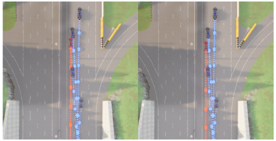(b) KING Lane Merger Scenario

(c) KING Collision Avoidance

Figure 10: Demonstration of safe driving methods: (a) InterFuser [8] processes multisensorial information to detect adversarial events, which are then used by the controller to constrain driving actions within safe sets. (b) KING [6] improves collision avoidance using scenario generation. The image shows the ego vehicle (shown in red) maintaining a safe distance during a lane merge in the presence of an adversarial agent (shown in blue). (c) In the same context, the image illustrates the vehicle slowing down to avoid collision.

8 Safety

Table 4: END-TO-END DRIVING TESTING TO ENSURE SAFETY

Methods	Summary	Literature
	Generating neuron coverage to identify false actions	[120]
	Designing an diverse and critical unsafe test cases	[6]
Search-based testing	Objective function to search safety sensitive output	[84]
	Place the original object with an adversarial one	[103]
Optimization- based attack	Virtual obstacles to generate adversarial attack in natural environment	[22]
	Generate the adversarial realistic-looking representations based on images	[121]
	Generate pedestrian augmentation from inserting pedestrians in image	[122]
GAN-based attack	Designing an objective function to search for the diverse unsafe test cases	[8]

Table 5: END-TO-END TESTING ORACLE MEASURES CORRECT CONTROL DECISION AT DIFFERENT SCENARIOS

Test Oracle	Detail	Literature
Metamorphic testing	The control signal should not get alter in different condition	[6]
Differential testing	The End-to-End system must give the same safe control for same scenario	[50]
Model-based oracle	Predicting the critical scenario that cause system failure	[23]

Table 6: POPULAR SAFETY METRICS USED FOR SAFETY EVALUATION OF DRIVING SYSTEM

Classification	Critical Metrics	Literature	Description
	Time to Collision (TTC)	[123]	It defines the minimum time interval that the two agents will collide
	Worst Time to Collision (WTTC)	[124]	The WTTC metric is an extension of the traditional TTC that takes numerous traces of actors into consideration
	Time to Maneuver (TTM)	[123]	The TTM yields the latest time in the range [0, TTC] at which an expert actor may conduct a movement that avoids a collision
	Time to React (TTR)	[120]	TTR metric provides an approximation of the latest time before a reaction is necessary
Temporal metrics	Time Headway (THW)	[123]	The THW measure determines the amount of time it will take an actor to get to the location of other vehicle
	Deceleration Safety Time (DST)	[125]	It calculates the deceleration required to maintain the safe distance
	Stopping Distance (SD)	[126]	Minimum stopping distance at the time of deceleration
	Crash Potential Index (CPI)	[127]	It measures the probability that the vehicle cannot avoid the collision by deceleration
Non-Temporal metrics	Conflict Index (CI)	[127]	It estimates the collision probability and the severity factors

Ensuring safety in End-to-End autonomous driving systems is a complex challenge. While these systems offer high-performance potential, several considerations and approaches are essential for maintaining safety throughout the pipeline. First, training the system with diverse and high-quality data that covers a wide range of scenarios, including rare and critical situations. Hanselmann et al. [6], Chen et al. [10], Chitta et al. [7], Xiao et al. [14], and Ohn-Bar et al. [49] demonstrate that training on critical scenarios helps the system learn robust and safe behaviors and prepares it for environmental conditions and potential hazards. These scenarios include unprotected turnings at intersections, pedestrians emerging from occluded regions, aggressive lane-changing, and other safety heuristics, as shown in Fig. 10(b) and Fig. 10(c). Hanselmann et al. [6] focus on improving robustness by inducing adversarial scenarios (collision scenarios) and collecting an observation-waypoint dataset using experts, which is then used to fine-tune the policy.

Integrating safety constraints and rules into the End-to-End system is another vital aspect. The system can prioritize safe behavior by incorporating safety considerations during learning or post-processing system outputs. Safety constraints include a safety cost function [80, 82, 65, 90], avoiding unsafe maneuvers [11, 19], and collision avoidance strategies [58, 13, 50]. Zeng et al. [84] define the cost volume responsible for safe planning; Kendall et al. [59] propose a practical safety reward function for safety-sensitive outputs. Li et al. [55] and Hu et al. [20] demonstrate safety by utilizing the Safety Cost function that penalizes jerk, significant acceleration, and safety violations. To avoid unsafe maneuvers, Zhang et al. [51] eliminate unsafe waypoints, and Shao et al. [8] introduce InterFuser (Fig. 10(a)), which constrains only the actions within the safety set and steers only the safest action. The above constraints ensure that the system operates within predefined safety boundaries.

Implementing additional safety modules and testing mechanisms (Tables 4, 5) enhances the system’s safety. Real-time monitoring of the system’s behavior allows for detecting abnormalities or deviations from safe operation. Hu et al. [9], Renz et al. [18], Wu et al. [13], and Hawke et al. [24] implement a planner that identifies collision-free routes, reduces possible infractions, and compensates for potential failures or inaccuracies. Renz et al. [18] use a rule-based expert algorithm for their planner, while Wu et al. [13] propose a trajectory + control model that predicts a safe trajectory over the long horizon. Hu et al. [9] also employ a goal planner to ensure safety. Codevilla et al. [23] demonstrate the system’s ability to respond appropriately and return the vehicle to a safe state when encountering potential inconsistencies. Similarly, Zhao et al. [50] incorporate stop intentions to help avoid hazardous traffic situations and respond appropriately. These mechanisms ensure that the system can detect and respond to abnormal or unexpected situations, thereby reducing the risk of accidents or unsafe behavior.

Adversarial attack [22] methods, as shown in the Table 4, are utilized in driving testing to evaluate the correctness of the output control signal. These testing methodologies aim to identify vulnerabilities and assess the robustness against adversaries. The End-to-End testing oracle (Table 5) determines the correct control decision within a given scenario. Metamorphic testing tackles the oracle problem by verifying the consistency of the steering angle [6] across various weather and lighting conditions. It provides a reliable way to ensure that the steering angle remains stable and unaffected by these factors. Differential testing [50] exposes inconsistencies among different DNN models by comparing their inference results for the same scenario. If the models produce different outcomes, it indicates unexpected behavior and potential issues in the system. The model-based oracle employs a trained probabilistic model to assess and predict potential risks [23] in real scenarios. By monitoring the environment, it can identify situations that the system may not adequately handle.

Safety metrics provide quantitative measures to evaluate the performance of autonomous driving systems and assess how well the system functions in terms of safety. Time to Collision (TTC), Conflict Index (CI), Crash Potential Index (CPI), Time to React (TTR), and others are some of the metrics that can provide additional objective comparisons between the safety performance of various approaches and identify areas that require improvement. A description of these metrics is provided in Table 6.

9 Explainability

Explainability [128] refers to the ability to understand the logic of an agent and is focused on how a user interprets the relationships between the input and output of a model. It encompasses two main concepts: interpretability, which relates to the understandability of explanations, and completeness, which pertains to exhaustively defining the behavior of the model through explanations. Choi et al. [129] distinguish three types of confidence in autonomous vehicles: transparency, which refers to the person’s ability to foresee and comprehend vehicle operation; technical competence, which relates to understanding vehicle performance; and situation management, which involves the notion that the user can regain vehicle control at any time. According to Haspiel et al. [130], explanations play a crucial role when humans are involved, as the ability to explain an autonomous vehicle’s actions significantly impacts consumer trust, which is essential for the widespread acceptance of this technology.

Figure 11: Categorization of Explainability Approaches.

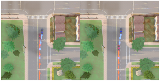
In the context of explainability for end-to-end autonomous driving systems, we can categorize explanation approaches into two main types (Fig. 11): local explanations and global explanations. A local explanation aims to describe the rationale behind the predictions of the model. On the other hand, global explanations aim to comprehensively comprehend the model’s behavior by describing the underlying knowledge. As of now, there is no available research on global explanations in the context of end-to-end autonomous driving [131]. Therefore, future research should focus on addressing this gap.

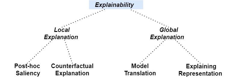
(a) PlanT agent’s attention

(b) InterFuser failure explanation

Figure 12: Explainability Methods: (a) PlanT [18] visualization showing the attention given to the agent in various scenarios. (b) Using InterFuser [8], failure cases can be visualized by integrating three RGB views and a predicted object density map. The orange boxes indicate objects that pose a collision risk to the ego-vehicle. The object density map offers predictions for the current traffic scene ($t_{0}$) and future traffic scenes at 1-second ($t_{1}$) and 2-second ($t_{2}$) intervals.

9.1 Local explanations

A local explanation describes why the model $f$ produces its prediction $y=f(x)$ given an input $x$. There are two approaches: in 9.1.1, we determine which visual region has the most impact, and in 9.1.2, we identify the factors that caused the model to predict $f(x)$.

9.1.1 Post-hoc saliency methods

A post-hoc saliency technique attempts to explain which portions of the input space have the most effect on the model’s output. These approaches provide a saliency map that illustrates the locations where the model made the most significant decisions.

Post-hoc saliency methods primarily focus on the perception component of the driving architecture. Bojarski et al. [132] introduced the first post-hoc saliency approach for visualizing the impact of inputs in autonomous driving. Renz et al. [18] proposed the PlanT method (Fig. 12(a)), which utilizes an attention mechanism for post-hoc saliency visualization to provide object-level representations using the attention weights of the transformer to identify the most relevant objects. Mori et al. [133] proposed an attention mechanism that utilizes the model’s predictions of steering angle and throttle. These local predictions are employed as visual attention maps and combined with learned parameters using a linear combination to make the final decision. While attention-based methods are often believed to improve the transparency of neural networks, it should be noted that learned attention weights may exhibit weak correlations with several features. The attention weights can provide accurate predictions when measuring different input features during driving. Overall, evaluating the post-hoc effectiveness of attention mechanisms is challenging and often relies on subjective human evaluation.

9.1.2 Counterfactual explanation

Saliency approaches focus on answering the ‘where’ question, identifying influential input locations for the model’s decision. In contrast, counterfactual explanations address the ‘what’ question by seeking small changes in the input that alter the model’s prediction. Counterfactual analysis aims to identify features $X$ within the input $x$ that led to the outcome $y=f(x)$ by creating a new input instance $x^{\prime}$ where $X$ is modified, resulting in a different outcome $y^{\prime}$. The modified input instance $x^{\prime}$ serves as the counterfactual example, and $y^{\prime}$ represents the contrasting class, such as ‘What changes in the traffic scenario would cause the vehicle to stop moving?’ It could be a red light.

Since the input space consists of semantic dimensions and is modifiable, assessing the causality of input components is straightforward. Li et al. [125] proposed a causal inference technique for identifying risky objects. Steex [134] developed a counterfactual method that modifies the style of the region to explain the visual model. The semantic input provides a high-level object representation, making it more interpretable compared to pixel-level representations.

Bansal et al. [135] explore the underlying causes of particular outcomes by examining the ChauffeurNet model using manually crafted inputs that involve omitting particular objects.

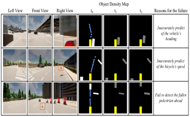
In End-to-End driving, the steering, throttle, and brake driving outputs can be complemented with auxiliary outputs such as the occupancy and interpretable semantics to demonstrate a specific degree of counterfactual understandability. Chitta et al. [7] introduce an auxiliary output (semantics map) that employs the A* planner to address a counterfactual inquiry of “What is the possibility of a collision without braking". Shao et al. [8] designed a system, as shown in Fig. 12(b), which infers counterfactual reasoning for the potential failures with the assistance of an intermediate object density map. Sadat et al. [90] generate a probabilistic semantic occupancy map over space and time, capturing the positions of diverse road agents. Occupancy maps provide a counterfactual explanation as they act as an intermediary representation to the motion planning system, higher occupancy probabilities will discourages the maneuvers while lower occupancy will encourage them.

9.2 Global explanations

Global explanations aim to provide an overall understanding of a model’s behavior by describing the knowledge it possesses. They are classified into model translation (9.2.1) and representation explanation techniques (9.2.2) for analyzing global explanations.

9.2.1 Model translation

The objective of model translation is to transfer the information from the original model to a different model that is inherently interpretable. This involves training an explainable model to mimic the input-output relationship. Recent studies have explored translating deep learning models into decision trees [136], rule-based models [137], or causal models [138]. However, one limitation of this approach is the potential discrepancies between the interpretable translated model and the original self-driving model.

9.2.2 Explaining representations

Explaining representations aims to explain the information captured by the model’s structures at various scales. Zhang et al. [139] and Bau et al. [140] make efforts to gain insights into what the neurons capture. The activation of a neuron can be understood by examining input patterns that maximize its activity. For example, one can sample the input using gradient ascent [141] or generative networks [142]. Tian et al. [120] employ the concept of neuron coverage to identify false actions that could potentially lead to fatalities. They partition the input space based on neuron coverage, assuming that inputs with the same neuron coverage will result in the same model decision. Their objective is to increase neuron coverage through transformations such as linear changes in image intensity and affine transformations like rotation and convolution.

Table 7: CARLA AUTONOMOUS DRIVING LEADERBOARD 1.0 SUBMISSION UNTIL AUGUST 2023

Rank	Submission	DS	RC	IP	CP	CV	CL	RLI	SSI	OI	RD	AB	Type
		%	%	[0,1]	infractions/km								E/M
1	ReasonNet [16]	79.95	89.89	0.89	0.02	0.13	0.01	0.08	0.00	0.04	0.00	0.33	E
1	InterFuser [8]	76.18	88.23	0.84	0.04	0.37	0.14	0.22	0.00	0.13	0.00	0.43	E
2	TCP [13]	75.14	85.63	0.87	0.00	0.32	0.00	0.09	0.00	0.04	0.00	0.54	E
3	TF++ [71]	66.32	78.57	0.84	0.00	0.50	0.00	0.01	0.00	0.12	0.00	0.71	E
3	LAV [10]	61.85	94.46	0.64	0.04	0.70	0.02	0.17	0.00	0.25	0.09	0.10	E
4	TransFuser [7]	61.18	86.69	0.71	0.04	0.81	0.01	0.05	0.00	0.23	0.00	0.43	E
5	Latent TransFuser [7]	45.20	66.31	0.72	0.02	1.11	0.02	0.05	0.00	0.16	0.00	1.82	E
6	GRIAD [100]	36.79	61.85	0.60	0.00	2.77	0.41	0.48	0.00	1.39	1.11	0.84	E
7	TransFuser+ [7]	34.58	69.84	0.56	0.04	0.70	0.03	0.75	0.00	0.18	0.00	2.41	E
8	World on Rails [99]	31.37	57.65	0.56	0.61	1.35	1.02	0.79	0.00	0.96	1.69	0.47	E
9	MaRLn [53]	24.98	46.97	0.52	0.00	2.33	2.47	0.55	0.00	1.82	1.44	0.94	E
10	NEAT [12]	21.83	41.71	0.65	0.04	0.74	0.62	0.70	0.00	2.68	0.00	5.22	E
11	AIM-MT [12]	19.38	67.02	0.39	0.18	1.53	0.12	1.55	0.00	0.35	0.00	2.11	E
12	TransFuser [14]	16.93	51.82	0.42	0.91	1.09	0.19	1.26	0.00	0.57	0.00	1.96	E
13	CNN-Planner [143]	15.40	50.05	0.41	0.08	4.67	0.42	0.35	0.00	2.78	0.12	4.63	M
14	Learning by [48]	8.94	17.54	0.73	0.00	0.40	1.16	0.71	0.00	1.52	0.03	4.69	E
15	MaRLn [53]	5.56	24.72	0.36	0.77	3.25	13.23	0.85	0.00	10.73	2.97	11.41	E
16	CILRS [12]	5.37	14.40	0.55	2.69	1.48	2.35	1.62	0.00	4.55	4.14	4.28	E
17	CaRINA [144]	4.56	23.80	0.41	0.01	7.56	51.52	20.64	0.00	14.32	0.00	10055.99	M

• Route Completion (RC), Infraction Score/penalty (IS), Driving score (DS), Collisions pedestrians (CP)/(PC), Collisions vehicles (CV), Collisions layout (CL)/(LC), Red light infractions (RLI), Red light violation (RV), Stop sign infractions (SSI), Off-road infractions (OI), Route deviations (RD), Agent blocked (AB), End-to-End Architecture (E), Modular Architecture (M).

10 Evaluation

The evaluation of the End-to-End system consists of open-loop evaluation and closed-loop evaluation. The open loop is assessed using real-world benchmark datasets such as KITTI [110] and nuScenes [145]. It compares the system’s driving behavior with expert actions and measures the deviation. Measures such as MinADE, MinFDE [9], L2 error [20], and collision rate [84] are some of the evaluation metrics presented in Table LABEL:literature. In contrast the closed-loop evaluation directly assesses the system in controlled real-world or simulated settings by allowing it to drive independently and learn safe driving maneuvers.

In the open-loop evaluation of End-to-End driving systems, the system’s inputs, such as camera images or LiDAR data, are provided to the system. The resulting outputs, such as steering commands and vehicle speed, are evaluated against predefined driving behaviors. The evaluation metrics commonly used in the open-loop evaluation include measures of the system’s ability to follow the desired trajectory or driving behaviors, such as the mean squared error [50], L2 [9, 82] between the predicted and actual trajectories or the percentage of time the system remains within a certain distance of the desired trajectory [13]. Other evaluation metrics may also be employed to assess the system’s performance in specific driving scenarios [14, 6], such as the system’s capability to navigate intersections, handle obstacles, or perform lane changes. The open loop provides faster initial assessment based on functionalities and is also helpful for testing specific components or behaviors in isolation. However, they inherit drawbacks from the benchmark datasets as they cannot generalize to wider geographical distribution.

Most of the recent End-to-End systems are evaluated in closed-loop settings such as LEADERBOARD and NOCRASH [109]. Table 7 compares all the state-of-the-art methods on the CARLA public leaderboard. The CARLA leaderboard analyzes autonomous driving systems in unanticipated environments. Vehicles are tasked with completing a set of specified routes, incorporating risky scenarios such as unexpectedly crossing pedestrians or sudden lane changes. The leaderboard measures how far the vehicle has successfully traveled on the given Town route within a time constraint and how many times it has incurred infractions. Several metrics provide a comprehensive understanding of the driving system, which are mentioned below:

• Route Completion (RC): [7, 10, 18, 13, 8] measures the percentage of the distance that an agent can complete.

• Infraction Score/penalty (IS): [14, 51, 12] is a geometric series that tracks infractions and aggregates the infraction penalties. It measures how often an agent drives without causing infractions.

• Driving score (DS): [54, 52, 49] is a primary metric calculated as the multiplication of the route completion and the infraction penalty. It measures the route completion rate weighted by infractions per route.

There are specific metrics that evaluate infractions; each metric has penalty coefficients applied every time an infraction takes place. Collisions with pedestrians, collisions with other vehicles, collisions with static elements, collisions layout, red light infractions, stop sign infractions, and off-road infractions are some of the metrics used [143]. Closed-loop evaluation provides dynamic testing adaptability where one can provide customized configuration and sensor settings. The feedback loop in it allows for iterative refinement, enabling the system to learn and improve from mistakes and experiences. However, several challenges are associated with closed-loop. These include the complexity of the initial setup and the domain gap, which might require additional fine-tuning.

11 Datasets and simulator

11.1 Datasets

In End-to-End models, the quality and richness of data are critical aspects of model training. Instead of using different hyperparameters, the training data is the most crucial factor influencing the model’s performance. The amount of information fed into the model determines the kind of outcomes it produces. We summarized the self-driving dataset based on their sensor modalities, including camera, LiDAR, GNSS, and dynamics. The content of the datasets includes urban driving, traffic, and different road conditions. Weather conditions also influence the model’s performance. Some datasets, such as ApolloScape [146], capture all weather conditions from sunny to snowy. The details are provided in Table 8.

11.2 Simulators and toolsets

Standard testing of End-to-End driving and learning pipelines requires advanced software simulators to process information and make conclusions for their various functionalities. Experimenting with such driving systems is expensive, and conducting tests on public roads is heavily restricted. Simulation environments assist in training specific algorithms/modules before road testing. Simulators like Carla [109] offer flexibility to simulate the environment based on experimental requirements, including weather conditions, traffic flow, road agents, etc. Simulators play a crucial role in generating safety-critical scenarios and contribute to model generalization for detecting and preventing such scenarios.

Widely used platforms for training End-to-End driving pipelines are compared in Table 9. MATLAB/Simulink [147] is used for various settings; it contains efficient plot functions and has the ability to co-simulate with other software, such as CarSim [148], which simplifies the creation of different settings. PreScan [149] can mimic real-world environments, including weather conditions, which MATLAB and CarSim lack. It also supports the MATLAB Simulink interface, making modeling more effective. Gazebo [150] is well-known for its high versatility and easy connection with ROS. In contrast to the CARLA and LGSVL [151] simulators, creating a simulated environment with Gazebo requires mechanical effort. CARLA and LGSVL offer high-quality simulation frameworks that require a GPU processing unit to operate at a decent speed and frame rate. CARLA is built on the Unreal Engine, while LGSVL is based on the Unity game engine. The API allows users to access various capabilities in CARLA and LGSVL, from developing customizable sensors to map generation. LGSVL generally links to the driving stack through various bridges, and CARLA allows built-in bridge connections via ROS and Autoware.

12 Future research directions

This section will highlight the possible research directions that can drive future advancements in the domain from the perspective of learning principles, safety, explainability, and others.

12.1 Learning robustness

Current research in End-to-End autonomous driving mainly focuses on reinforcement learning (Section 6.2) and imitation learning (Section 6.1) methods. RL trains agents by interacting with simulated environments, while IL learns from expert agents without extensive environmental interaction. However, challenges like distribution shift in IL and computational instability in RL highlight the need for further improvements.

12.2 Enhanced safety

Ensuring the behavioral safety of vehicles and accurately predicting uncertain behaviors are key aspects in safety research as discussed in Section 8. An effective system should be capable of handling various driving situations, contributing to comfortable and reliable transportation. To facilitate the widespread adoption of End-to-End approaches, it is essential to refine safety constraints and enhance their effectiveness.

12.3 Advancing model explainability

The lack of interpretability poses a new challenge for the advancement of End-to-End driving. However, ongoing efforts (Section 9) are being made to address this issue by designing and generating interpretable features. These efforts have shown promising improvements in both performance and explainability. However, further exploration is required in global explanation strategies, including designing novel approaches to explain model actions leading to failures and suggesting potential solutions. Future research can also explore ways to improve feedback mechanisms, allowing users to understand the decision-making process and infuse confidence in the reliability of End-to-End driving systems.

12.4 Collaboration perception systems

Vehicles can communicate directly utilizing collaborative perception to observe surroundings beyond their line of sight and field of view. This approach addresses issues related to occlusion and limited receptive fields. Cooperative or collaborative perception enables vehicles in the same area to communicate and jointly assess the scene.

Table 8: CUMULATIVE LIST OF DATASETS WITH THEIR DYNAMICS FOR END-TO-END TRAINING

Datasets

Year

Sensors Modalities

Content

Weather

Size

Location

License

Cameras

LiDAR

GNSS

Steering

Speed, Acceleration

Navigational command

Route planner

Obstacles

Traffic

Raods

Sunny

Rain

Snow or Fog

Udacity [152]

2016

✓

✓

✓

✓

✓

✓

✓

✓

5h

Mountain View

MIT

Drive360 [153]

2019

✓

✓

✓

✓

✓

✓

✓

✓

55h

Switzerland

Academic

Comma.ai 2016 [154]

2016

✓

✓

✓

✓

✓

7h 15min

San Francisco

CC BY-NC-SA 3.0

Comma.ai 2019 [155]

2019

✓

✓

✓

✓

✓

30h

San Jose California

MIT

BDD 100 [156]

2018

✓

✓

✓

✓

✓

✓

1100h

US

Berkley

Oxford RobotCar [2]

2019

✓

✓

✓

✓

✓

✓

✓

✓

214h

Oxford

CC BY-NC-SA 4.0

HDD [157]

2018

✓

✓

✓

✓

✓

✓

✓

✓

✓

104h

San Francisco

Academic

Brain4Cars [158]

2016

✓

✓

✓

✓

✓

1180 miles

US

Academic

Li-Vi [159, 160]

2018

✓

✓

✓

✓

✓

10h

China

Academic

DDD17 [161]

2017

✓

✓

✓

✓

✓

✓

✓

✓

12h

Switzerland, Germany

CC-BY-NC-SA-4.0

A2D2 [162]

2020

✓

✓

✓

✓

✓

✓

✓

✓

390k frames

South of Germany

CC BY-ND 4.0

nuScenes [145]

2019

✓

✓

✓

✓

✓

✓

5.5h

Boston, Singapore

Non-commercial

Waymo [163]

2019

✓

✓

✓

✓

✓

✓

✓

5.5h

California

Non-commercial

H3D [46]

2019

✓

✓

✓

✓

✓

✓

N/A

Japan

Academic

HAD [164]

2019

✓

✓

✓

✓

✓

✓

30h

San Francisco

Academic

BIT [165]

2015

✓

✓

✓

9850 frames

Beijing

Academics

UA-DETRAC [166]

2015

✓

✓

✓

140k frames

Beijing, Tianjing

CC BY-NC-SA 3.0

DFG [167]

2019

✓

✓

✓

✓

7k+8k

Slovenia

CC BY-NC-SA 4.0

Bosch [168]

2017

✓

✓

✓

8334 frames

Germany

Research Only

Tencent 100k [169]

2016

✓

✓

✓

30k

China

CC-BY-NC

LISA [170]

2012

✓

✓

✓

20k

California

Research Only

STSD [171]

2011

✓

✓

✓

2503 frames

Sweden

CC BY-SA 4.0

GTSRB [172]

2013

✓

✓

✓

✓

50k

Germany

CC0 1.0

KUL [173]

2013

✓

✓

✓

16k

Flanders

CC0 1.0

Caltech [174]

2009

✓

✓

✓

10 hours

California

CC4.0

CamVid [175]

2009

✓

✓

✓

✓

✓

22 min, 14 s

Cambridge

Academic

Ford[176]

2018

✓

✓

✓

✓

66 km

Michigan

CC-BY-NC-SA 4.0

KITTI [110]

2013

✓

✓

✓

✓

✓

✓

✓

43 k

Karlsruhe

Apache License 2.0

CityScapes [177]

2016

✓

✓

✓

✓

✓

20+5 K frams

Germany, France, Scotland

Apache License 2.0

Mapillary [178]

2017

✓

✓

✓

✓

✓

25000 frames

Germany

Research Only

ApolloScape [146]

2018

✓

✓

✓

✓

✓

✓

✓

147 k frames

China

Non-commercial

VERI-Wild [179]

2019

✓

✓

✓

✓

125, 280 hours

China

Research Only

D2 -City [180]

2019

✓

✓

✓

✓

✓

10000 video

China

Research Only

DriveSeg [181]

2020

✓

✓

✓

✓

✓

500 minutes

Massachusetts

CC BY-NC 4.0

Table 9: PROMINENT SIMULATORS USED FOR CREATING VIRTUAL ENVIRONMENTS FOR END-TO-END SYSTEMS

Simulators	MATLAB [147]	CarSim [148]	PreScan [149]	CARLA [109]	LGSVL [151]
Sensors support	✓	✓	✓	✓	✓
Weather condition			✓	✓	✓
Camera calibration	✓		✓	✓
Path planning	✓	✓	✓	✓	✓
Vehicle dynamics	✓	✓	✓	✓	✓
Virtual environment		✓	✓	✓	✓
Infrastructure fabrication	✓	✓	✓	✓	✓
Scenarios simulator	✓	✓	✓	✓	✓
Ground truth	✓			✓	✓
Simulator connectivity	✓	✓	✓	✓	✓
System scalability				✓	✓
Open source				✓	✓
System stable	✓	✓	✓	✓	✓
System portable	✓	✓	✓	✓	✓
API flexibility	✓	✓		✓	✓

Cooperative perception methods [182, 183, 184] include V2V (vehicle-to-vehicle), V2I (vehicle-to-infrastructure), and V2X (vehicle-to-everything) modes. Future works should focus on enhancing the transmission efficiency within collaboration systems while safeguarding data privacy.

12.5 Large language and vision models

Large vision models have emerged as a prominent trend in AI. By harnessing the advancements in these models, various domains can benefit from their integration. Visual prompts have become essential aids for understanding visuals across diverse domains and enhancing model capacity for interpreting visual data. Presently, SAM-Track [185] for object tracking and VIMA [186] for robot action manipulation showcase potential, implying that these large models can optimize visual recognition systems. Moreover, we can effectively utilize large language and vision models through transfer learning, domain adaptation, and fine-tuning. We can transfer insights from a larger model to a smaller one, emphasizing the importance of compact transfer of knowledge and applying it to novel tasks while upholding performance and adaptability, especially in contexts like autonomous driving. Future efforts must focus on designing large vision models tailored explicitly to autonomous driving and prompt fine-tuning to guide tasks related to perception and control.

13 Conclusion

Over the past few years, there has been significant interest in End-to-End autonomous driving due to the simplicity of its design compared to conventional modular autonomous driving. We develop a taxonomy based on modalities, learning, and training methodology and investigate the potential of leveraging domain adaptation approaches to optimize the training process. Furthermore, the paper explores evaluation framework that encompasses both open and closed-loop assessments, enabling a comprehensive analysis of system performance. To facilitate further research and development in the domain, we compile a summarized list of advancements, publicly available datasets and simulators. The paper also explores potential solutions proposed by different articles regarding safety and explainability. Despite the impressive performance of End-to-End approaches, there is a need for continued exploration and improvement in safety and interpretability to achieve broader technology acceptance.

pranav_photo.jpeg Pranav Singh Chib is a Ph.D. candidate in the Computer Science and Engineering department at the Indian Institute of Technology, Roorkee. He holds a Post-Graduate Computer Science and Technology Specialization from Jawaharlal Nehru University, New Delhi. Pranav’s research interests lie in machine learning, computer vision, and autonomous driving. His ongoing doctoral studies focus on contributing to advancements in autonomous driving and deep learning.

psingh.jpg Pravendra Singh received his Ph.D. degree from IIT Kanpur. He is currently an Assistant Professor in the CSE department at IIT Roorkee, India. His research interests include deep learning, machine learning, computer vision, and artificial intelligence. He has published papers at internationally reputable conferences and journals, including IEEE TPAMI, IJCV, CVPR, ECCV, NeurIPS, AAAI, IJCAI, IJCV, Pattern Recognition, Neural Networks, Knowledge-Based Systems, Neurocomputing, and others.

References

- [1] C. Chen, A. Seff, A. Kornhauser, J. Xiao, Deepdriving: Learning affordance for direct perception in autonomous driving, in: Proceedings of the IEEE international conference on computer vision, 2015, pp. 2722–2730.
- [2] W. Maddern, G. Pascoe, C. Linegar, P. Newman, 1 year, 1000 km: The oxford robotcar dataset, The International Journal of Robotics Research 36 (1) (2017) 3–15.
- [3] N. Akai, L. Y. Morales, T. Yamaguchi, E. Takeuchi, Y. Yoshihara, H. Okuda, T. Suzuki, Y. Ninomiya, Autonomous driving based on accurate localization using multilayer lidar and dead reckoning, in: 2017 IEEE 20th International Conference on Intelligent Transportation Systems (ITSC), IEEE, 2017, pp. 1–6.
- [4] J. Kong, M. Pfeiffer, G. Schildbach, F. Borrelli, Kinematic and dynamic vehicle models for autonomous driving control design, in: 2015 IEEE intelligent vehicles symposium (IV), IEEE, 2015, pp. 1094–1099.
- [5] P. Zhao, J. Chen, Y. Song, X. Tao, T. Xu, T. Mei, Design of a control system for an autonomous vehicle based on adaptive-pid, International Journal of Advanced Robotic Systems 9 (2) (2012) 44.
- [6] N. Hanselmann, K. Renz, K. Chitta, A. Bhattacharyya, A. Geiger, King: Generating safety-critical driving scenarios for robust imitation via kinematics gradients, in: Computer Vision–ECCV 2022: 17th European Conference, Tel Aviv, Israel, October 23–27, 2022, Proceedings, Part XXXVIII, Springer, 2022, pp. 335–352.
- [7] K. Chitta, A. Prakash, B. Jaeger, Z. Yu, K. Renz, A. Geiger, Transfuser: Imitation with transformer-based sensor fusion for autonomous driving, IEEE Transactions on Pattern Analysis and Machine Intelligence (2022).
- [8] H. Shao, L. Wang, R. Chen, H. Li, Y. Liu, Safety-enhanced autonomous driving using interpretable sensor fusion transformer, in: Conference on Robot Learning, PMLR, 2023, pp. 726–737.
- [9] Y. Hu, J. Yang, L. Chen, K. Li, C. Sima, X. Zhu, S. Chai, S. Du, T. Lin, W. Wang, L. Lu, X. Jia, Q. Liu, J. Dai, Y. Qiao, H. Li, Planning-oriented autonomous driving, in: Proceedings of the IEEE/CVF Conference on Computer Vision and Pattern Recognition, 2023.
- [10] D. Chen, P. Krähenbühl, Learning from all vehicles, in: Proceedings of the IEEE/CVF Conference on Computer Vision and Pattern Recognition, 2022, pp. 17222–17231.
- [11] Q. Zhang, Z. Peng, B. Zhou, Learning to drive by watching youtube videos: Action-conditioned contrastive policy pretraining, in: Computer Vision–ECCV 2022: 17th European Conference, Tel Aviv, Israel, October 23–27, 2022, Proceedings, Part XXVI, Springer, 2022, pp. 111–128.
- [12] K. Chitta, A. Prakash, A. Geiger, Neat: Neural attention fields for end-to-end autonomous driving, in: Proceedings of the IEEE/CVF International Conference on Computer Vision, 2021, pp. 15793–15803.
- [13] P. Wu, X. Jia, L. Chen, J. Yan, H. Li, Y. Qiao, Trajectory-guided control prediction for end-to-end autonomous driving: A simple yet strong baseline, in: NeurIPS, 2022.
- [14] A. Prakash, K. Chitta, A. Geiger, Multi-modal fusion transformer for end-to-end autonomous driving, in: Proceedings of the IEEE/CVF Conference on Computer Vision and Pattern Recognition, 2021, pp. 7077–7087.
- [15] P. Wu, L. Chen, H. Li, X. Jia, J. Yan, Y. Qiao, Policy pre-training for end-to-end autonomous driving via self-supervised geometric modeling, arXiv preprint arXiv:2301.01006 (2023).
- [16] H. Shao, L. Wang, R. Chen, S. L. Waslander, H. Li, Y. Liu, Reasonnet: End-to-end driving with temporal and global reasoning, in: Proceedings of the IEEE/CVF Conference on Computer Vision and Pattern Recognition, 2023, pp. 13723–13733.
- [17] Y. Xiao, F. Codevilla, D. P. Bustamante, A. M. Lopez, Scaling self-supervised end-to-end driving with multi-view attention learning, arXiv preprint arXiv:2302.03198 (2023).
- [18] K. Renz, K. Chitta, O.-B. Mercea, A. S. Koepke, Z. Akata, A. Geiger, Plant: Explainable planning transformers via object-level representations, in: CoRL 2022 Workshop on Learning, Perception, and Abstraction for Long-Horizon Planning.
- [19] X. Jia, P. Wu, L. Chen, J. Xie, C. He, J. Yan, H. Li, Think twice before driving: Towards scalable decoders for end-to-end autonomous driving, in: Proceedings of the IEEE/CVF Conference on Computer Vision and Pattern Recognition, 2023, pp. 21983–21994.
- [20] S. Hu, L. Chen, P. Wu, H. Li, J. Yan, D. Tao, St-p3: End-to-end vision-based autonomous driving via spatial-temporal feature learning, in: Computer Vision–ECCV 2022: 17th European Conference, Tel Aviv, Israel, October 23–27, 2022, Proceedings, Part XXXVIII, Springer, 2022, pp. 533–549.
- [21] Q. Li, Z. Peng, H. Wu, L. Feng, B. Zhou, Human-ai shared control via policy dissection, Advances in Neural Information Processing Systems 35 (2022) 8853–8867.
- [22] H. Wu, S. Yunas, S. Rowlands, W. Ruan, J. Wahlstrom, "adversarial driving: Attacking end-to-end autonomous driving", in ieee intelligent vehicles symposium (iv) (2023).
- [23] F. Codevilla, E. Santana, A. M. López, A. Gaidon, Exploring the limitations of behavior cloning for autonomous driving, in: Proceedings of the IEEE/CVF International Conference on Computer Vision, 2019, pp. 9329–9338.
- [24] J. Hawke, R. Shen, C. Gurau, S. Sharma, D. Reda, N. Nikolov, P. Mazur, S. Micklethwaite, N. Griffiths, A. Shah, et al., Urban driving with conditional imitation learning, in: 2020 IEEE International Conference on Robotics and Automation (ICRA), IEEE, 2020, pp. 251–257.
- [25] E. Yurtsever, J. Lambert, A. Carballo, K. Takeda, A survey of autonomous driving: Common practices and emerging technologies, IEEE access 8 (2020) 58443–58469.
- [26] L. Le Mero, D. Yi, M. Dianati, A. Mouzakitis, A survey on imitation learning techniques for end-to-end autonomous vehicles, IEEE Transactions on Intelligent Transportation Systems 23 (9) (2022) 14128–14147.
- [27] Z. Zhu, H. Zhao, A survey of deep rl and il for autonomous driving policy learning, IEEE Transactions on Intelligent Transportation Systems 23 (9) (2021) 14043–14065.
- [28] A. Tampuu, T. Matiisen, M. Semikin, D. Fishman, N. Muhammad, A survey of end-to-end driving: Architectures and training methods, IEEE Transactions on Neural Networks and Learning Systems 33 (4) (2020) 1364–1384.
- [29] L. Chen, P. Wu, K. Chitta, B. Jaeger, A. Geiger, H. Li, End-to-end autonomous driving: Challenges and frontiers, arXiv 2306.16927 (2023).
- [30] J. Levinson, J. Askeland, J. Becker, J. Dolson, D. Held, S. Kammel, J. Z. Kolter, D. Langer, O. Pink, V. Pratt, et al., Towards fully autonomous driving: Systems and algorithms, in: 2011 IEEE intelligent vehicles symposium (IV), IEEE, 2011, pp. 163–168.
- [31] C. Urmson, J. Anhalt, D. Bagnell, C. Baker, R. Bittner, M. Clark, J. Dolan, D. Duggins, T. Galatali, C. Geyer, et al., Autonomous driving in urban environments: Boss and the urban challenge, Journal of field Robotics 25 (8) (2008) 425–466.
- [32] J. Wei, J. M. Snider, J. Kim, J. M. Dolan, R. Rajkumar, B. Litkouhi, Towards a viable autonomous driving research platform, in: 2013 IEEE Intelligent Vehicles Symposium (IV), IEEE, 2013, pp. 763–770.
- [33] H. Somerville, P. Lienert, A. Sage, Uber’s use of fewer safety sensors prompts questions after arizona crash, Business news, Reuters (2018).
- [34] J. Ziegler, P. Bender, M. Schreiber, H. Lategahn, T. Strauss, C. Stiller, T. Dang, U. Franke, N. Appenrodt, C. G. Keller, et al., Making bertha drive—an autonomous journey on a historic route, IEEE Intelligent transportation systems magazine 6 (2) (2014) 8–20.
- [35] S. Kuutti, S. Fallah, K. Katsaros, M. Dianati, F. Mccullough, A. Mouzakitis, A survey of the state-of-the-art localization techniques and their potentials for autonomous vehicle applications, IEEE Internet of Things Journal 5 (2) (2018) 829–846.
- [36] L. Bergamini, Y. Ye, O. Scheel, L. Chen, C. Hu, L. Del Pero, B. Osiński, H. Grimmett, P. Ondruska, Simnet: Learning reactive self-driving simulations from real-world observations, in: 2021 IEEE International Conference on Robotics and Automation (ICRA), IEEE, 2021, pp. 5119–5125.
- [37] C.-F. Lin, A. G. Ulsoy, D. J. LeBlanc, Vehicle dynamics and external disturbance estimation for vehicle path prediction, IEEE Transactions on Control Systems Technology 8 (3) (2000) 508–518.
- [38] T. Phan-Minh, E. C. Grigore, F. A. Boulton, O. Beijbom, E. M. Wolff, Covernet: Multimodal behavior prediction using trajectory sets, in: Proceedings of the IEEE/CVF Conference on Computer Vision and Pattern Recognition, 2020, pp. 14074–14083.
- [39] T. Gilles, S. Sabatini, D. Tsishkou, B. Stanciulescu, F. Moutarde, Home: Heatmap output for future motion estimation, in: 2021 IEEE International Intelligent Transportation Systems Conference (ITSC), IEEE, 2021, pp. 500–507.
- [40] M. Ye, T. Cao, Q. Chen, Tpcn: Temporal point cloud networks for motion forecasting, in: Proceedings of the IEEE/CVF Conference on Computer Vision and Pattern Recognition (CVPR), 2021, pp. 11318–11327.
- [41] M. Ye, T. Cao, Q. Chen, Tpcn: Temporal point cloud networks for motion forecasting, in: Proceedings of the IEEE/CVF Conference on Computer Vision and Pattern Recognition, 2021, pp. 11318–11327.
- [42] Y. Liu, J. Zhang, L. Fang, Q. Jiang, B. Zhou, Multimodal motion prediction with stacked transformers, in: Proceedings of the IEEE/CVF Conference on Computer Vision and Pattern Recognition, 2021, pp. 7577–7586.
- [43] J. Gu, C. Sun, H. Zhao, Densetnt: End-to-end trajectory prediction from dense goal sets, in: Proceedings of the IEEE/CVF International Conference on Computer Vision, 2021, pp. 15303–15312.
- [44] H. Song, D. Luan, W. Ding, M. Y. Wang, Q. Chen, Learning to predict vehicle trajectories with model-based planning, in: Conference on Robot Learning, PMLR, 2022, pp. 1035–1045.
- [45] D. Wei, H. Sun, B. Li, J. Lu, W. Li, X. Sun, S. Hu, Human joint kinematics diffusion-refinement for stochastic motion prediction, arXiv preprint arXiv:2210.05976 (2022).
- [46] A. Patil, S. Malla, H. Gang, Y.-T. Chen, The h3d dataset for full-surround 3d multi-object detection and tracking in crowded urban scenes, in: 2019 International Conference on Robotics and Automation (ICRA), IEEE, 2019, pp. 9552–9557.
- [47] D. A. Pomerleau, Alvinn: An autonomous land vehicle in a neural network, Advances in neural information processing systems 1 (1988).
- [48] D. Chen, B. Zhou, V. Koltun, P. Krähenbühl, Learning by cheating, in: Conference on Robot Learning, PMLR, 2020, pp. 66–75.
- [49] E. Ohn-Bar, A. Prakash, A. Behl, K. Chitta, A. Geiger, Learning situational driving, in: Proceedings of the IEEE/CVF Conference on Computer Vision and Pattern Recognition, 2020, pp. 11296–11305.
- [50] A. Zhao, T. He, Y. Liang, H. Huang, G. Van den Broeck, S. Soatto, Sam: Squeeze-and-mimic networks for conditional visual driving policy learning, in: Conference on Robot Learning, PMLR, 2021, pp. 156–175.
- [51] J. Zhang, E. Ohn-Bar, Learning by watching, in: Proceedings of the IEEE/CVF Conference on Computer Vision and Pattern Recognition, 2021, pp. 12711–12721.
- [52] D. Chen, V. Koltun, P. Krähenbühl, Learning to drive from a world on rails, in: Proceedings of the IEEE/CVF International Conference on Computer Vision, 2021, pp. 15590–15599.
- [53] M. Toromanoff, E. Wirbel, F. Moutarde, End-to-end model-free reinforcement learning for urban driving using implicit affordances, in: Proceedings of the IEEE/CVF conference on computer vision and pattern recognition, 2020, pp. 7153–7162.
- [54] Z. Zhang, A. Liniger, D. Dai, F. Yu, L. Van Gool, End-to-end urban driving by imitating a reinforcement learning coach, in: Proceedings of the IEEE/CVF international conference on computer vision, 2021, pp. 15222–15232.
- [55] Q. Li, Z. Peng, B. Zhou, Efficient learning of safe driving policy via human-ai copilot optimization, in: International Conference on Learning Representations.
- [56] Z. Peng, Q. Li, C. Liu, B. Zhou, Safe driving via expert guided policy optimization, in: Conference on Robot Learning, PMLR, 2022, pp. 1554–1563.
- [57] Y. Zhao, K. Wu, Z. Xu, Z. Che, Q. Lu, J. Tang, C. H. Liu, Cadre: A cascade deep reinforcement learning framework for vision-based autonomous urban driving, in: Proceedings of the AAAI Conference on Artificial Intelligence, Vol. 36, 2022, pp. 3481–3489.
- [58] J. Zhang, Z. Huang, E. Ohn-Bar, Coaching a teachable student, in: Proceedings of the IEEE/CVF Conference on Computer Vision and Pattern Recognition, 2023, pp. 7805–7815.
- [59] A. Kendall, J. Hawke, D. Janz, P. Mazur, D. Reda, J.-M. Allen, V.-D. Lam, A. Bewley, A. Shah, Learning to drive in a day, in: 2019 International Conference on Robotics and Automation (ICRA), 2019, pp. 8248–8254. doi:10.1109/ICRA.2019.8793742.
- [60] A. Prakash, A. Behl, E. Ohn-Bar, K. Chitta, A. Geiger, Exploring data aggregation in policy learning for vision-based urban autonomous driving, in: Proceedings of the IEEE/CVF Conference on Computer Vision and Pattern Recognition, 2020, pp. 11763–11773.
- [61] K. Ishihara, A. Kanervisto, J. Miura, V. Hautamaki, Multi-task learning with attention for end-to-end autonomous driving, in: Proceedings of the IEEE/CVF Conference on Computer Vision and Pattern Recognition, 2021, pp. 2902–2911.
- [62] Y. Xiao, F. Codevilla, A. Gurram, O. Urfalioglu, A. M. López, Multimodal end-to-end autonomous driving, IEEE Transactions on Intelligent Transportation Systems 23 (1) (2020) 537–547.
- [63] P. Hu, A. Huang, J. Dolan, D. Held, D. Ramanan, Safe local motion planning with self-supervised freespace forecasting, in: Proceedings of the IEEE/CVF Conference on Computer Vision and Pattern Recognition (CVPR), 2021, pp. 12732–12741.
-
[64]
P. Cai, S. Wang, H. Wang, M. Liu,
Carl-lead:
Lidar-based end-to-end autonomous driving with contrastive deep reinforcement
learning, ArXiv abs/2109.08473 (2021).
URL https://api.semanticscholar.org/CorpusID:237563170 -
[65]
W. Zeng, S. Wang, R. Liao, Y. Chen, B. Yang, R. Urtasun,
Dsdnet: Deep
structured self-driving network, in: European Conference on Computer Vision,
2020.
URL https://api.semanticscholar.org/CorpusID:221112477 - [66] Q. Zhang, M. Tang, R. Geng, F. Chen, R. Xin, L. Wang, Mmfn: Multi-modal-fusion-net for end-to-end driving, in: 2022 IEEE/RSJ International Conference on Intelligent Robots and Systems (IROS), IEEE, 2022, pp. 8638–8643.
- [67] T. Bailey, H. Durrant-Whyte, Simultaneous localization and mapping (slam): Part ii, IEEE robotics & automation magazine 13 (3) (2006) 108–117.
- [68] A. Shenoi, M. Patel, J. Gwak, P. Goebel, A. Sadeghian, H. Rezatofighi, R. Martin-Martin, S. Savarese, Jrmot: A real-time 3d multi-object tracker and a new large-scale dataset, in: 2020 IEEE/RSJ International Conference on Intelligent Robots and Systems (IROS), IEEE, 2020, pp. 10335–10342.
- [69] M. Liang, B. Yang, Y. Chen, R. Hu, R. Urtasun, Multi-task multi-sensor fusion for 3d object detection, in: Proceedings of the IEEE/CVF Conference on Computer Vision and Pattern Recognition, 2019, pp. 7345–7353.
- [70] M. Liang, B. Yang, S. Wang, R. Urtasun, Deep continuous fusion for multi-sensor 3d object detection, in: Proceedings of the European conference on computer vision (ECCV), 2018, pp. 641–656.
- [71] B. Jaeger, K. Chitta, A. Geiger, Hidden biases of end-to-end driving models (2023).
- [72] Y. Zhou, P. Sun, Y. Zhang, D. Anguelov, J. Gao, T. Ouyang, J. Guo, J. Ngiam, V. Vasudevan, End-to-end multi-view fusion for 3d object detection in lidar point clouds, in: Conference on Robot Learning, PMLR, 2020, pp. 923–932.
- [73] I. Sobh, L. Amin, S. Abdelkarim, K. Elmadawy, M. Saeed, O. Abdeltawab, M. Gamal, A. El Sallab, End-to-end multi-modal sensors fusion system for urban automated driving (2018).
- [74] B. Zhou, P. Krähenbühl, V. Koltun, Does computer vision matter for action?, Science Robotics 4 (30) (2019) eaaw6661.
- [75] C. Hubschneider, A. Bauer, M. Weber, J. M. Zöllner, Adding navigation to the equation: Turning decisions for end-to-end vehicle control, in: 2017 IEEE 20th International Conference on Intelligent Transportation Systems (ITSC), IEEE, 2017, pp. 1–8.
- [76] F. Codevilla, M. Müller, A. López, V. Koltun, A. Dosovitskiy, End-to-end driving via conditional imitation learning, in: 2018 IEEE international conference on robotics and automation (ICRA), IEEE, 2018, pp. 4693–4700.
- [77] X. Liang, T. Wang, L. Yang, E. Xing, Cirl: Controllable imitative reinforcement learning for vision-based self-driving, in: Proceedings of the European conference on computer vision (ECCV), 2018, pp. 584–599.
- [78] S. Wang, J. Qin, M. Li, Y. Wang, Flowdrivenet: An end-to-end network for learning driving policies from image optical flow and lidar point flow, in: 2021 IEEE International Conference on Robotics and Automation (ICRA), IEEE, 2021, pp. 1861–1867.
- [79] R. Fong, M. Patrick, A. Vedaldi, Understanding deep networks via extremal perturbations and smooth masks, in: Proceedings of the IEEE/CVF international conference on computer vision, 2019, pp. 2950–2958.
- [80] A. Cui, S. Casas, A. Sadat, R. Liao, R. Urtasun, Lookout: Diverse multi-future prediction and planning for self-driving, in: Proceedings of the IEEE/CVF International Conference on Computer Vision, 2021, pp. 16107–16116.
- [81] W. Zeng, W. Luo, S. Suo, A. Sadat, B. Yang, S. Casas, R. Urtasun, End-to-end interpretable neural motion planner, in: Proceedings of the IEEE/CVF Conference on Computer Vision and Pattern Recognition, 2019, pp. 8660–8669.
- [82] S. Casas, A. Sadat, R. Urtasun, Mp3: A unified model to map, perceive, predict and plan, in: Proceedings of the IEEE/CVF Conference on Computer Vision and Pattern Recognition, 2021, pp. 14403–14412.
- [83] N. Rhinehart, R. McAllister, S. Levine, Deep imitative models for flexible inference, planning, and control, in: International Conference on Learning Representations.
- [84] W. Zeng, W. Luo, S. Suo, A. Sadat, B. Yang, S. Casas, R. Urtasun, End-to-end interpretable neural motion planner, in: Proceedings of the IEEE/CVF Conference on Computer Vision and Pattern Recognition, 2019, pp. 8660–8669.
- [85] X. Chen, H. Ma, J. Wan, B. Li, T. Xia, Multi-view 3d object detection network for autonomous driving, in: Proceedings of the IEEE conference on Computer Vision and Pattern Recognition, 2017, pp. 1907–1915.
- [86] I. Kim, H. Lee, J. Lee, E. Lee, D. Kim, Multi-task learning with future states for vision-based autonomous driving, in: Proceedings of the Asian Conference on Computer Vision, 2020.
- [87] M. Bain, C. Sammut, A framework for behavioural cloning., in: Machine Intelligence 15, 1995, pp. 103–129.
- [88] J. Cui, H. Qiu, D. Chen, P. Stone, Y. Zhu, Coopernaut: End-to-end driving with cooperative perception for networked vehicles, in: Proceedings of the IEEE/CVF Conference on Computer Vision and Pattern Recognition, 2022, pp. 17252–17262.
- [89] S. Ross, G. Gordon, D. Bagnell, A reduction of imitation learning and structured prediction to no-regret online learning, in: Proceedings of the fourteenth international conference on artificial intelligence and statistics, JMLR Workshop and Conference Proceedings, 2011, pp. 627–635.
- [90] A. Sadat, S. Casas, M. Ren, X. Wu, P. Dhawan, R. Urtasun, Perceive, predict, and plan: Safe motion planning through interpretable semantic representations, in: Computer Vision–ECCV 2020: 16th European Conference, Glasgow, UK, August 23–28, 2020, Proceedings, Part XXIII 16, Springer, 2020, pp. 414–430.
- [91] D. Sadigh, S. Sastry, S. A. Seshia, A. D. Dragan, Planning for autonomous cars that leverage effects on human actions., in: Robotics: Science and systems, Vol. 2, Ann Arbor, MI, USA, 2016, pp. 1–9.
- [92] B. D. Ziebart, A. L. Maas, J. A. Bagnell, A. K. Dey, et al., Maximum entropy inverse reinforcement learning., in: Aaai, Vol. 8, Chicago, IL, USA, 2008, pp. 1433–1438.
- [93] G. Wang, H. Niu, D. Zhu, J. Hu, X. Zhan, G. Zhou, A versatile and efficient reinforcement learning framework for autonomous driving, arXiv preprint arXiv:2110.11573 (2021).
- [94] R. S. Sutton, A. G. Barto, Reinforcement learning: An introduction, MIT press, 2018.
- [95] L. Chen, X. Hu, B. Tang, Y. Cheng, Conditional dqn-based motion planning with fuzzy logic for autonomous driving, IEEE Transactions on Intelligent Transportation Systems 23 (4) (2020) 2966–2977.
- [96] J. Chen, S. E. Li, M. Tomizuka, Interpretable end-to-end urban autonomous driving with latent deep reinforcement learning, IEEE Transactions on Intelligent Transportation Systems 23 (6) (2021) 5068–5078.
- [97] X. Zhang, Y. Jiang, Y. Lu, X. Xu, Receding-horizon reinforcement learning approach for kinodynamic motion planning of autonomous vehicles, IEEE Transactions on Intelligent Vehicles 7 (3) (2022) 556–568.
- [98] X. Liang, T. Wang, L. Yang, E. Xing, Cirl: Controllable imitative reinforcement learning for vision-based self-driving, in: Proceedings of the European conference on computer vision (ECCV), 2018, pp. 584–599.
- [99] D. Chen, V. Koltun, P. Krähenbühl, Learning to drive from a world on rails, in: Proceedings of the IEEE/CVF International Conference on Computer Vision, 2021, pp. 15590–15599.
- [100] R. Chekroun, M. Toromanoff, S. Hornauer, F. Moutarde, Gri: General reinforced imitation and its application to vision-based autonomous driving, in: NeurIPS 2021, Machine Learning for Autonomous Driving Workshop, 2021.
- [101] Y. Chen, W. Li, C. Sakaridis, D. Dai, L. V. Gool, Domain adaptive faster r-cnn for object detection in the wild (2018). arXiv:1803.03243.
- [102] H. Zhang, G. Luo, Y. Tian, K. Wang, H. He, F.-Y. Wang, A virtual-real interaction approach to object instance segmentation in traffic scenes, IEEE Transactions on Intelligent Transportation Systems 22 (2) (2021) 863–875. doi:10.1109/TITS.2019.2961145.
[103]
L. Zhang, T. Wen, J. Min, J. Wang, D. Han, J. Shi,
Learning object placement
by inpainting for compositional data augmentation, in: A. Vedaldi,
H. Bischof, T. Brox, J.-M. Frahm (Eds.), Computer Vision - ECCV 2020 - 16th
European Conference, Glasgow, UK, August 23-28, 2020, Proceedings, Part XIII,
Vol. 12358 of Lecture Notes in Computer Science, Springer, 2020, pp.
566–581.
doi:10.1007/978-3-030-58601-0_34.
URL https://doi.org/10.1007/978-3-030-58601-0_34 - [104] Y. Chen, F. Rong, S. Duggal, S. Wang, X. Yan, S. Manivasagam, S. Xue, E. Yumer, R. Urtasun, Geosim: Realistic video simulation via geometry-aware composition for self-driving, in: Proceedings of the IEEE/CVF conference on computer vision and pattern recognition, 2021, pp. 7230–7240.
- [105] A. Vobeckỳ, D. Hurych, M. Uřičář, P. Pérez, J. Sivic, Artificial dummies for urban dataset augmentation, in: Proceedings of the AAAI Conference on Artificial Intelligence, Vol. 35, 2021, pp. 2692–2700.
- [106] A. E. Sallab, I. Sobh, M. Zahran, M. Shawky, Unsupervised neural sensor models for synthetic lidar data augmentation (2019). arXiv:1911.10575.
- [107] J. Fang, D. Zhou, F. Yan, T. Zhao, F. Zhang, Y. Ma, L. Wang, R. Yang, Augmented lidar simulator for autonomous driving, IEEE Robotics and Automation Letters 5 (2) (2020) 1931–1938. doi:10.1109/LRA.2020.2969927.
- [108] S. Manivasagam, S. Wang, K. Wong, W. Zeng, M. Sazanovich, S. Tan, B. Yang, W.-C. Ma, R. Urtasun, Lidarsim: Realistic lidar simulation by leveraging the real world (2020). arXiv:2006.09348.
- [109] A. Dosovitskiy, G. Ros, F. Codevilla, A. Lopez, V. Koltun, Carla: An open urban driving simulator, in: Conference on robot learning, PMLR, 2017, pp. 1–16.
- [110] A. Geiger, P. Lenz, C. Stiller, R. Urtasun, Vision meets robotics: The kitti dataset, The International Journal of Robotics Research 32 (11) (2013) 1231–1237.
- [111] P. Wu, L. Chen, H. Li, X. Jia, J. Yan, Y. Qiao, Policy pre-training for autonomous driving via self-supervised geometric modeling, in: International Conference on Learning Representations, 2023.
- [112] A. Hu, G. Corrado, N. Griffiths, Z. Murez, C. Gurau, H. Yeo, A. Kendall, R. Cipolla, J. Shotton, Model-based imitation learning for urban driving, Advances in Neural Information Processing Systems 35 (2022) 20703–20716.
- [113] J. Park, Y. Seo, C. Liu, L. Zhao, T. Qin, J. Shin, T.-Y. Liu, Object-aware regularization for addressing causal confusion in imitation learning, Advances in Neural Information Processing Systems 34 (2021) 3029–3042.
- [114] A. Bewley, J. Rigley, Y. Liu, J. Hawke, R. Shen, V.-D. Lam, A. Kendall, Learning to drive from simulation without real world labels, in: 2019 International conference on robotics and automation (ICRA), IEEE, 2019, pp. 4818–4824.
- [115] S. Hecker, D. Dai, L. Van Gool, Learning accurate, comfortable and human-like driving, arXiv preprint arXiv:1903.10995 (2019).
- [116] X. Pan, Y. You, Z. Wang, C. Lu, Virtual to real reinforcement learning for autonomous driving (2017). arXiv:1704.03952.
- [117] B. Osiński, A. Jakubowski, P. Miłoś, P. Zięcina, C. Galias, S. Homoceanu, H. Michalewski, Simulation-based reinforcement learning for real-world autonomous driving (2020). arXiv:1911.12905.
- [118] R. Mitchell, J. Fletcher, J. Panerati, A. Prorok, Multi-vehicle mixed reality reinforcement learning for autonomous multi-lane driving, in: Proceedings of the 19th International Conference on Autonomous Agents and MultiAgent Systems, 2020, pp. 1928–1930.
[119]
A. Stocco, B. Pulfer, P. Tonella,
Mind the gap! a study on
the transferability of virtual versus physical-world testing of autonomous
driving systems, IEEE Transactions on Software Engineering 49 (4) (2023)
1928–1940.
doi:10.1109/tse.2022.3202311.
URL https://doi.org/10.1109.2Ftse.2022.3202311 - [120] Y. Tian, K. Pei, S. Jana, B. Ray, Deeptest: Automated testing of deep-neural-network-driven autonomous cars, in: Proceedings of the 40th international conference on software engineering, 2018, pp. 303–314.
- [121] I. Goodfellow, J. Pouget-Abadie, M. Mirza, B. Xu, D. Warde-Farley, S. Ozair, A. Courville, Y. Bengio, Generative adversarial networks, Communications of the ACM 63 (11) (2020) 139–144.
- [122] X. Ouyang, Y. Cheng, Y. Jiang, C.-L. Li, P. Zhou, Pedestrian-synthesis-gan: Generating pedestrian data in real scene and beyond (2018). arXiv:1804.02047.
- [123] B. Weng, S. J. Rao, E. Deosthale, S. Schnelle, F. Barickman, Model predictive instantaneous safety metric for evaluation of automated driving systems, in: 2020 IEEE Intelligent Vehicles Symposium (IV), IEEE, 2020, pp. 1899–1906.
- [124] W. Wachenfeld, P. Junietz, R. Wenzel, H. Winner, The worst-time-to-collision metric for situation identification, in: 2016 IEEE intelligent vehicles symposium (IV), IEEE, 2016, pp. 729–734.
- [125] C. Li, S. H. Chan, Y.-T. Chen, Who make drivers stop? towards driver-centric risk assessment: Risk object identification via causal inference, in: 2020 IEEE/RSJ International Conference on Intelligent Robots and Systems (IROS), IEEE, 2020, pp. 10711–10718.
- [126] G. Li, Y. Li, S. Jha, T. Tsai, M. Sullivan, S. K. S. Hari, Z. Kalbarczyk, R. Iyer, Av-fuzzer: Finding safety violations in autonomous driving systems, in: 2020 IEEE 31st international symposium on software reliability engineering (ISSRE), IEEE, 2020, pp. 25–36.
- [127] W. K. Alhajyaseen, The integration of conflict probability and severity for the safety assessment of intersections, Arabian Journal for Science and Engineering 40 (2015) 421–430.
- [128] A. Rosenfeld, A. Richardson, Explainability in human–agent systems, Autonomous Agents and Multi-Agent Systems 33 (2019) 673–705.
- [129] J. K. Choi, Y. G. Ji, Investigating the importance of trust on adopting an autonomous vehicle, International Journal of Human-Computer Interaction 31 (10) (2015) 692–702.
- [130] J. Haspiel, N. Du, J. Meyerson, L. P. Robert Jr, D. Tilbury, X. J. Yang, A. K. Pradhan, Explanations and expectations: Trust building in automated vehicles, in: Companion of the 2018 ACM/IEEE international conference on human-robot interaction, 2018, pp. 119–120.
- [131] Y. Tian, K. Pei, S. Jana, B. Ray, Deeptest: Automated testing of deep-neural-network-driven autonomous cars. 2017, arXiv preprint arXiv:1708.08559 (2017).
- [132] M. Bojarski, A. Choromanska, K. Choromanski, B. Firner, L. J. Ackel, U. Muller, P. Yeres, K. Zieba, Visualbackprop: Efficient visualization of cnns for autonomous driving, in: 2018 IEEE International Conference on Robotics and Automation (ICRA), IEEE, 2018, pp. 4701–4708.
- [133] K. Mori, H. Fukui, T. Murase, T. Hirakawa, T. Yamashita, H. Fujiyoshi, Visual explanation by attention branch network for end-to-end learning-based self-driving, in: 2019 IEEE intelligent vehicles symposium (IV), IEEE, 2019, pp. 1577–1582.
- [134] P. Jacob, É. Zablocki, H. Ben-Younes, M. Chen, P. Pérez, M. Cord, Steex: steering counterfactual explanations with semantics, in: Computer Vision–ECCV 2022: 17th European Conference, Tel Aviv, Israel, October 23–27, 2022, Proceedings, Part XII, Springer, 2022, pp. 387–403.
- [135] M. Bansal, A. Krizhevsky, A. Ogale, Chauffeurnet: Learning to drive by imitating the best and synthesizing the worst, arXiv preprint arXiv:1812.03079 (2018).
- [136] N. Frosst, G. Hinton, Distilling a neural network into a soft decision tree, arXiv preprint arXiv:1711.09784 (2017).
- [137] J. R. Zilke, E. Loza Mencía, F. Janssen, Deepred–rule extraction from deep neural networks, in: Discovery Science: 19th International Conference, DS 2016, Bari, Italy, October 19–21, 2016, Proceedings 19, Springer, 2016, pp. 457–473.
- [138] M. Harradon, J. Druce, B. Ruttenberg, Causal learning and explanation of deep neural networks via autoencoded activations, arXiv preprint arXiv:1802.00541 (2018).
- [139] Q.-s. Zhang, S.-C. Zhu, Visual interpretability for deep learning: a survey, Frontiers of Information Technology & Electronic Engineering 19 (1) (2018) 27–39.
- [140] D. Bau, B. Zhou, A. Khosla, A. Oliva, A. Torralba, Network dissection: Quantifying interpretability of deep visual representations, in: Proceedings of the IEEE conference on computer vision and pattern recognition, 2017, pp. 6541–6549.
- [141] K. Simonyan, A. Vedaldi, A. Zisserman, Deep inside convolutional networks: visualising image classification models and saliency maps, in: Proceedings of the International Conference on Learning Representations (ICLR), ICLR, 2014.
- [142] A. Nguyen, A. Dosovitskiy, J. Yosinski, T. Brox, J. Clune, Synthesizing the preferred inputs for neurons in neural networks via deep generator networks, Advances in neural information processing systems 29 (2016).
- [143] L. Rosero, J. Silva, D. Wolf, F. Osório, Cnn-planner: A neural path planner based on sensor fusion in the bird’s eye view representation space for mapless autonomous driving, in: 2022 Latin American Robotics Symposium (LARS), 2022 Brazilian Symposium on Robotics (SBR), and 2022 Workshop on Robotics in Education (WRE), 2022, pp. 181–186. doi:10.1109/LARS/SBR/WRE56824.2022.9995888.
- [144] L. A. Rosero, I. P. Gomes, J. A. R. da Silva, T. C. dos Santos, A. T. M. Nakamura, J. Amaro, D. F. Wolf, F. S. Osório, A software architecture for autonomous vehicles: Team lrm-b entry in the first carla autonomous driving challenge (2020). arXiv:2010.12598.
- [145] H. Caesar, V. Bankiti, A. H. Lang, S. Vora, V. E. Liong, Q. Xu, A. Krishnan, Y. Pan, G. Baldan, O. Beijbom, nuscenes: A multimodal dataset for autonomous driving, in: Proceedings of the IEEE/CVF conference on computer vision and pattern recognition, 2020, pp. 11621–11631.
- [146] X. Huang, P. Wang, X. Cheng, D. Zhou, Q. Geng, R. Yang, The apolloscape open dataset for autonomous driving and its application, IEEE transactions on pattern analysis and machine intelligence 42 (10) (2019) 2702–2719.
[147]
Automated
Driving Toolbox.
URL https://in.mathworks.com/products/automated-driving.html -
[148]
Mechanical Simulation.
URL https://www.carsim.com/ -
[149]
PreScan.
URL https://in.mathworks.com/products/connections/product_detail/prescan.html -
[150]
Gazebo.
URL https://classic.gazebosim.org/ -
[151]
SVL Simulator by LG - Autonomous
and Robotics real-time sensor Simulation, LiDAR, Camera simulation
for ROS1, ROS2, Autoware, Baidu Apollo. Perception, Planning,
Localization, SIL and HIL Simulation, Open Source and Free.
URL https://www.svlsimulator.com/ - [152] Udacity: Public driving dataset, https://github.com/udacity/self-driving-car/tree/master/datasets (2017).
- [153] S. Hecker, D. Dai, L. Van Gool, End-to-end learning of driving models with surround-view cameras and route planners, in: Proceedings of the European Conference on Computer Vision (ECCV), 2018, pp. 435–453.
- [154] E. Santana, G. Hotz, Learning a driving simulator, arXiv preprint arXiv:1608.01230 (2016).
- [155] H. Schafer, E. Santana, A. Haden, R. Biasini, A commute in data: The comma2k19 dataset, arXiv preprint arXiv:1812.05752 (2018).
- [156] F. Yu, H. Chen, X. Wang, W. Xian, Y. Chen, F. Liu, V. Madhavan, T. Darrell, Bdd100k: A diverse driving dataset for heterogeneous multitask learning, in: Proceedings of the IEEE/CVF conference on computer vision and pattern recognition, 2020, pp. 2636–2645.
- [157] V. Ramanishka, Y.-T. Chen, T. Misu, K. Saenko, Toward driving scene understanding: A dataset for learning driver behavior and causal reasoning, in: Proceedings of the IEEE Conference on Computer Vision and Pattern Recognition, 2018, pp. 7699–7707.
- [158] A. Jain, H. S. Koppula, B. Raghavan, S. Soh, A. Saxena, Car that knows before you do: Anticipating maneuvers via learning temporal driving models, in: Proceedings of the IEEE International Conference on Computer Vision, 2015, pp. 3182–3190.
- [159] Y. Chen, J. Wang, J. Li, C. Lu, Z. Luo, H. Xue, C. Wang, Lidar-video driving dataset: Learning driving policies effectively, in: Proceedings of the IEEE Conference on Computer Vision and Pattern Recognition, 2018, pp. 5870–5878.
- [160] Large-scale driving behavior dataset, http://www.dbehavior.net/index.html.
- [161] Y. Hu, J. Binas, D. Neil, S.-C. Liu, T. Delbruck, Ddd20 end-to-end event camera driving dataset: Fusing frames and events with deep learning for improved steering prediction, in: 2020 IEEE 23rd International Conference on Intelligent Transportation Systems (ITSC), IEEE, 2020, pp. 1–6.
- [162] J. Geyer, Y. Kassahun, M. Mahmudi, X. Ricou, R. Durgesh, A. S. Chung, L. Hauswald, V. H. Pham, M. Mhlegg, S. Dorn, et al., A2d2: Aev autonomous driving dataset, https://www.audi-electronics-venture.com/aev/web/en/driving-dataset.html (2019).
- [163] P. Sun, H. Kretzschmar, X. Dotiwalla, A. Chouard, V. Patnaik, P. Tsui, J. Guo, Y. Zhou, Y. Chai, B. Caine, et al., Scalability in perception for autonomous driving: Waymo open dataset, arXiv (2019) arXiv–1912.
- [164] J. Kim, T. Misu, Y.-T. Chen, A. Tawari, J. Canny, Grounding human-to-vehicle advice for self-driving vehicles, in: Proceedings of the IEEE Conference on Computer Vision and Pattern Recognition, 2019, pp. 10591–10599.
- [165] J. Sang, Z. Wu, P. Guo, H. Hu, H. Xiang, Q. Zhang, B. Cai, An improved yolov2 for vehicle detection, Sensors 18 (2018) 4272. doi:10.3390/s18124272.
- [166] L. Wen, D. Du, Z. Cai, Z. Lei, M.-C. Chang, H. Qi, J. Lim, M.-H. Yang, S. Lyu, Ua-detrac: A new benchmark and protocol for multi-object detection and tracking, Computer Vision and Image Understanding 193 (2020) 102907.
- [167] D. Tabernik, D. Skočaj, Deep Learning for Large-Scale Traffic-Sign Detection and Recognition, IEEE Transactions on Intelligent Transportation Systems (2019). doi:10.1109/TITS.2019.2913588.
- [168] K. Behrendt, L. Novak, A deep learning approach to traffic lights: Detection, tracking, and classification, in: Robotics and Automation (ICRA), 2017 IEEE International Conference on, IEEE.
- [169] Z. Zhu, D. Liang, S. Zhang, X. Huang, B. Li, S. Hu, Traffic-sign detection and classification in the wild, in: The IEEE Conference on Computer Vision and Pattern Recognition (CVPR), 2016.
- [170] M. B. Jensen, M. P. Philipsen, A. Møgelmose, T. B. Moeslund, M. M. Trivedi, Vision for looking at traffic lights: Issues, survey, and perspectives, IEEE Transactions on Intelligent Transportation Systems 17 (7) (2016) 1800–1815. doi:10.1109/TITS.2015.2509509.
- [171] F. Larsson, M. Felsberg, Using fourier descriptors and spatial models for traffic sign recognition, 2011, pp. 238–249. doi:10.1007/978-3-642-21227-7_23.
- [172] J. Stallkamp, M. Schlipsing, J. Salmen, C. Igel, The german traffic sign recognition benchmark: a multi-class classification competition, in: The 2011 international joint conference on neural networks, IEEE, 2011, pp. 1453–1460.
- [173] M. Mathias, R. Timofte, R. Benenson, L. Van Gool, Traffic sign recognition—how far are we from the solution?, in: The 2013 international joint conference on Neural networks (IJCNN), IEEE, 2013, pp. 1–8.
- [174] P. Dollár, C. Wojek, B. Schiele, P. Perona, Pedestrian detection: A benchmark, in: 2009 IEEE conference on computer vision and pattern recognition, IEEE, 2009, pp. 304–311.
- [175] G. J. Brostow, J. Fauqueur, R. Cipolla, Semantic object classes in video: A high-definition ground truth database, Pattern Recognition Letters 30 (2) (2009) 88–97.
[176]
S. Agarwal, A. Vora, G. Pandey, W. Williams, H. Kourous, J. McBride,
Ford multi-AV seasonal
dataset, The International Journal of Robotics Research 39 (12) (2020)
1367–1376.
doi:10.1177/0278364920961451.
URL https://doi.org/10.1177%2F0278364920961451 - [177] M. Cordts, M. Omran, S. Ramos, T. Rehfeld, M. Enzweiler, R. Benenson, U. Franke, S. Roth, B. Schiele, The cityscapes dataset for semantic urban scene understanding, in: Proceedings of the IEEE conference on computer vision and pattern recognition, 2016, pp. 3213–3223.
- [178] G. Neuhold, T. Ollmann, S. Rota Bulo, P. Kontschieder, The mapillary vistas dataset for semantic understanding of street scenes, in: Proceedings of the IEEE international conference on computer vision, 2017, pp. 4990–4999.
- [179] Y. Lou, Y. Bai, J. Liu, S. Wang, L. Duan, Veri-wild: A large dataset and a new method for vehicle re-identification in the wild, in: Proceedings of the IEEE/CVF conference on computer vision and pattern recognition, 2019, pp. 3235–3243.
- [180] Z. Che, G. Li, T. Li, B. Jiang, X. Shi, X. Zhang, Y. Lu, G. Wu, Y. Liu, J. Ye, D2-city: A large-scale dashcam video dataset of diverse traffic scenarios (2019). arXiv:1904.01975.
[181]
L. Ding, J. Terwilliger, R. Sherony, B. Reimer, L. Fridman,
Mit driveseg (manual) dataset
(2020).
doi:10.21227/mmke-dv03.
URL https://dx.doi.org/10.21227/mmke-dv03 - [182] Y. L. Yue Hu, R. Xu, W. Xie, Y. W. Siheng Chen, Collaboration helps camera overtake lidar in 3d detection, in: The IEEE/CVF Conference on Computer Vision and Pattern Recognition (CVPR), 2023.
- [183] H. Xiang, R. Xu, J. Ma, Hm-vit: Hetero-modal vehicle-to-vehicle cooperative perception with vision transformer, arXiv preprint arXiv:2304.10628 (2023).
- [184] B. Wang, L. Zhang, Z. Wang, Y. Zhao, T. Zhou, Core: Cooperative reconstruction for multi-agent perception, arXiv preprint arXiv:2307.11514 (2023).
- [185] Y. Cheng, L. Li, Y. Xu, X. Li, Z. Yang, W. Wang, Y. Yang, Segment and track anything, arXiv preprint arXiv:2305.06558 (2023).
- [186] Y. Jiang, A. Gupta, Z. Zhang, G. Wang, Y. Dou, Y. Chen, L. Fei-Fei, A. Anandkumar, Y. Zhu, L. Fan, Vima: General robot manipulation with multimodal prompts, arXiv preprint arXiv:2210.03094 (2022).