Continual Learning as
Computationally Constrained Reinforcement Learning

Abstract

An agent that accumulates knowledge to develop increasingly sophisticated skills over a long lifetime could advance the frontier of artificial intelligence capabilities. The design of such agents, which remains a long-standing challenge, is addressed by the subject of continual learning. This monograph clarifies and formalizes concepts of continual learning, introducing a framework and tools to stimulate further research. We also present a range of empirical case studies to illustrate the roles of forgetting, relearning, exploration, and auxiliary learning.

Metrics presented in previous literature for evaluating continual learning agents tend to focus on particular behaviors that are deemed desirable, such as avoiding catastrophic forgetting, retaining plasticity, relearning quickly, and maintaining low memory or compute footprints. In order to systematically reason about design and compare agents, a coherent, holistic objective that encompasses all such requirements would be helpful. To provide such an objective, we cast continual learning as reinforcement learning with limited compute resources. In particular, we pose the continual learning objective to be the maximization of infinite-horizon average reward subject to a computational constraint. Continual supervised learning, for example, is a special case of our general formulation where the reward is taken to be negative log-loss or accuracy. Among implications of maximizing average reward are that remembering all information from the past is unnecessary, forgetting non-recurring information is not “catastrophic,” and learning about how an environment changes over time is useful.

Computational constraints give rise to informational constraints in the sense that they limit the amount of information used to make decisions. A consequence is that, unlike more traditional framings of machine learning in which per-timestep regret vanishes as an agent accumulates information, the regret experienced in continual learning typically persists. Related to this is that a stationary environment can appear nonstationary due to informational constraints, creating a need for perpetual adaptation. Informational constraints also give rise to the familiar stability-plasticity dilemma, which we formalize in information-theoretic terms.

1 Introduction

Continual learning remains a long-standing challenge. An agent that efficiently accumulates knowledge to develop increasingly sophisticated skills over a long lifetime could advance the frontier of artificial intelligence capabilities [Hadsell et al., 2020, Khetarpal et al., 2022, Ring, 2005, Thrun and Pratt, 1998]. Success requires continuously ingesting new knowledge while retaining old knowledge that remains useful. Existing incremental machine learning techniques have failed to demonstrate this capability as they do not judiciously control what information they ingest, retain, or forget. Indeed, catastrophic forgetting (ejecting useful information from memory) and implasticity (forgoing useful new information) are recognized as obstacles to effective continual learning.

Traditional framings of machine learning view agents as acquiring knowledge about a fixed unknown latent variable. The aim is to develop methods that quickly learn about the latent variable, which we will refer to as the learning target, as data accumulates. For instance, in supervised learning, the learning target could be an unknown function mapping inputs to labels. In the reinforcement learning literature, the learning target is often taken to be the unknown transition matrix of a Markov decision process. With such traditional framings, an agent can be viewed as driving per-timestep regret – the performance shortfall relative to what could have been if the agent began with perfect knowledge of the learning target – to zero. If the agent is effective, regret vanishes as the agent accumulates knowledge. When regret becomes negligible, the agent is viewed as “done” with learning.

In contrast, continual learning addresses environments in which there may be no natural fixed learning target and an agent ought to never stop acquiring new knowledge. The need for continual learning can arise, for example, if properties of the agent’s data stream appear to change over time. To perform well, an agent must constantly adapt its behavior in response to these evolving patterns.

There is a large gap between the state of the art in continual learning and what may be possible, making the subject ripe for innovation. This difference becomes evident when examining an approach in common use, which entails periodically training a new model from scratch on buffered data. To crystalize this, consider as a hypothetical example an agent designed to trade stocks. At the end of each month, this agent trains a new neural network model from scratch on data observed over the preceding twelve months. Replacing the old, this new model then governs decisions over the next month. This agent serves as a simple baseline that affords opportunity for improvement. For example, training each month’s model from scratch is likely wasteful since it does not benefit from computation invested over previous months. Further, by limiting knowledge ingested by each model to that available from data acquired over the preceding twelve months, the agent forgoes the opportunity to acquire complex skills that might only be developed over a much longer duration.

While it ought to be possible to design more effective continual learning agents, how to go about that or even how to assess improvement remains unclear. Work on deep learning suggests that agent performance improves with increasing sizes of models, data sets, and inputs. However, computational resource requirements scale along with these and become prohibitive. A practically useful objective must account for computation. The primary goals of this monograph are to propose such an objective for continual learning and to understand key factors to consider in designing a performant continual learning agent. Rather than offer definitive methods, we aim to stimulate research toward identifying them.

Metrics presented in previous literature for evaluating continual learning agents tend to focus on particular behaviors that are deemed desirable, such as avoiding catastrophic forgetting, retaining plasticity, relearning quickly, and maintaining low memory or compute footprints [Ashley et al., 2021, Dohare et al., 2021, Fini et al., 2020, Kirkpatrick et al., 2017]. For instance, the most common evaluation metric measures prediction accuracy on previously seen tasks to study how well an agent retains past information [Wang et al., 2023]. However, the extent to which each of these behaviors matters is unclear. In order to systematically reason about design decisions and compare agents, a coherent, holistic objective that reflects and encompasses all such requirements would be helpful.

In this paper, we view continual learning under the lens of reinforcement learning [Agarwal et al., 2019, Bertsekas and Tsitsiklis, 1996, Meyn, 2022, Sutton and Barto, 2018, Szepesvári, 2010] to provide a formalism for what an agent is expected to accomplish. Specifically, we consider maximization of infinite-horizon average reward subject to a computational constraint. Average reward emphasizes long-term performance, which is suitable for the purpose of designing long-lived agents. The notion of maximizing average reward generalizes that of online average accuracy, as used in some literature on continual supervised learning [Cai et al., 2021, Ghunaim et al., 2023, Hammoud et al., 2023, Hu et al., 2022, Lin et al., 2021, Prabhu et al., 2023a, Xu et al., 2022].

As reflected by average reward, an agent should aim to perform well on an ongoing basis in the face of incoming data it receives from the environment. Importantly, remembering all information from the past is unnecessary, and forgetting non-recurring information is not “catastrophic.” An agent can perform well by remembering the subset that continues to remain useful. Although our objective relaxes the requirement of retaining all information to only retaining information useful in the future, even this remains difficult, or even impossible, in practice. Computational resources limit an agent’s capacity to retain and process information. The computational constraint in our continual learning objective reflects this gating factor. This is in line with recent work highlighting the need to consider computational costs in continual learning [Prabhu et al., 2023b].

The remainder of this monograph is organized as follows. In Section 2, we introduce our framing of continual learning as reinforcement learning with an objective of maximizing average reward subject to a computational constraint. In Section 3, we introduce information-theoretic tools inspired by Jeon et al. [2023], Lu et al. [2021] to offer a lens for studying agent behavior and performance. In Section 4, we interpret in these information-theoretic terms what it means for an agent to perpetually learn rather than drive regret to zero and be “done” with learning. This line of thought draws inspiration from Abel et al. [2023], who define a notion of convergence and associates continual learning with non-convergence. In Section 5, we formalize the concepts of stability and plasticity to enable coherent analysis of trade-offs between these conflicting goals. Finally, in Section 6, to highlight the implications of our continual learning objective, we study simulation results from a set of case studies. In the first case study, on continual supervised learning, we study the role of forgetting in relation to our continual learning objective. In the second and third case studies, on continual exploration and continual learning with delayed consequences, we study implications of nonstationarity and our objective on how an agent ought to explore and learn from delayed consequences.

2 An Objective for Continual Learning

Continual learning affords the never-ending acquisition of skills and knowledge [Ring, 1994]. An agent operating over an infinite time horizon can develop increasingly sophisticated skills, steadily building on what it learned earlier. On the other hand, due to computational resource constraints, as such an agent observes an ever-growing volume of data, it must forgo some skills to prioritize others. Designing a performant continual learning agent requires carefully trading off between these considerations. A suitable mathematical formulation of the design problem must account for that. While many metrics have been proposed in the literature, they have tended to focus on particular behaviors that are deemed desirable. A coherent, holistic objective would help researchers to systematically reason about design decisions and compare agents. In this section, we formulate such an objective in terms of computationally constrained reinforcement learning (RL).

The subject of RL addresses the design of agents that learn to achieve goals through interacting with an environment [Sutton and Barto, 2018]. As we will explain, the general RL formulation subsumes the many perspectives that appear in the continual learning literature. We review RL and its relation to continual learning, illustrating with examples. We will then highlight the critical role of computational constraints in capturing salient trade-offs that arise in continual learning. Imposing a computational constraint on the general RL formulation gives rise to a coherent objective for continual learning. Aside from formulating this objective, we reflect on several implications of framing continual learning in these terms.

2.1 Continual Interaction

We consider continual interaction across a general agent-environment interface as illustrated in Figure 1. At each time step $t=0,1,2,\ldots$, an agent executes an action $A_{t}$ and then observes a response $O_{t+1}$ produced by the environment. Actions take values in an action set $\mathcal{A}$. Observations take values in an observation set $\mathcal{O}$. The agent’s experience through time $t$ forms a sequence $H_{t}=(A_{0},O_{1},A_{1},O_{2},\ldots,A_{t-1},O_{t})$, which we refer to as its history. We denote the set of possible histories by $\mathcal{H}=\cup_{t=0}^{\infty}(\mathcal{A}\times\mathcal{O})^{t}$.

Figure 1: The agent-environment interface.

An environment is characterized by a triple $\mathcal{E}=(\mathcal{A},\mathcal{O},\rho)$, where $\rho$ is an observation probability distribution, which satisfies $\rho(\cdot|H_{t},A_{t})=\mathbb{P}(O_{t+1}\in\cdot|H_{t},A_{t})$. From the agent designer’s perspective, it is as though the environment samples $O_{t+1}$ from $\rho(\cdot|H_{t},A_{t})$.

The agent generates each action $A_{t}$ based on the previous history $H_{t}$. This behavior is characterized by a policy $\pi$, for which $\pi(\cdot|H_{t})=\mathbb{P}_{\pi}(A_{t}\in\cdot|H_{t})$. The subscript $\pi$ indicates the policy under which this probability is calculated. We refer to this policy, which characterizes the agent’s behavior, as the agent policy. While the agent may carry out sophisticated computations to determine each action, from the environment’s perspective, it is as though the agent simply samples $A_{t}$ from $\pi(\cdot|H_{t})$.

Note that we take event probabilities to represent uncertainty from the agent designer’s perspective. For example, $\mathbb{P}_{\pi}((A_{t},O_{t+1})\in\tilde{\mathcal{A}}\times\tilde{\mathcal{O}}|H_{t})$ is the designer’s subjective assessment of the chance that the next action-observation pair will fall in a set $\tilde{\mathcal{A}}\times\tilde{\mathcal{O}}$ conditioned on $H_{t}$, given that the agent implements $\pi$. We take the function $\rho$ to be deterministic, or equivalently, known to the designer. Note that the fact that $\rho$ is deterministic does not mean observations are fully determined by history and action. Rather, $\mathbb{P}(O_{t+1}\in\tilde{\mathcal{O}}|H_{t},A_{t})=\rho(\tilde{\mathcal{O}}|H_{t},A_{t})$ can lie between zero and one. With some abuse of notation, as shorthand, with singleton sets $\tilde{\mathcal{A}}$ and $\tilde{\mathcal{O}}$, we write $\pi(a|h)\equiv\pi(\{a\}|h)$ and $\rho(o|h,a)\equiv\rho(\{o\}|h,a)$. The following simple example offers a concrete instantiation of our formulation and notation.

Example 1.

(coin tossing) Consider an environment with two actions $\mathcal{A}=\{1,2\}$, each of which identifies a distinct coin. At each time $t$, an action $A_{t}$ selects a coin to toss next. Observations are binary, meaning $\mathcal{O}=\{0,1\}$, with $O_{t+1}$ indicating whether the selected coin lands heads. The coin biases $(p_{1},p_{2})$ are independent but initially unknown, and the designer’s uncertainty prescribes prior distributions. These environment dynamics are characterized by a function $\rho$ for which $\rho(1|h,a)$ is the probability that coin $a$ lands heads, regardless of the history $h$.

As a concrete special case, suppose the prior distribution over each coin’s bias is uniform over the unit interval. Then, at each time $t$, each bias $p_{a}$ is distributed $\mathrm{beta}(\alpha_{t,a},\beta_{t,a})$, with parameters initialized at $\alpha_{0,a}=\beta_{0,a}=1$ and updated according to $(\alpha_{t+1,A_{t}},\beta_{t+1,A_{t}})=(\alpha_{t,A_{t}}+O_{t+1},\beta_{t,A_{t}}+1-O_{t+1})$. Hence, $\rho(1|H_{t},A_{t})=\alpha_{t,A_{t}}/(\alpha_{t,A_{t}}+\beta_{t,A_{t}})$.

The form of interaction we consider is fully general; each observation can exhibit any sort of dependence on history. Notably, we do not assume that observations identify the state of the environment. While such an assumption – that the “environment is MDP,” so to speak – is common to much of the RL literature [Sutton and Barto, 2018], a number of researchers have advocated for the general action-observation interface, especially when treating design of generalist agents for complex environments [Daswani et al., 2013, 2014, Dong et al., 2022, Hutter, 2007, Lu et al., 2021, McCallum, 1995, Ring, 1994, 2005].

Note that we characterize the environment via a deterministic function $\rho$. Hence, the environment is known to the agent designer. This is in contrast to common formulations that treat the environment as unknown. As we will explain in Section 4, it is often more natural to treat environments of the sort that call for continual learning as known. Further, characterizing the environment as known never sacrifices generality, even when it is natural to treat the environment as unknown. In particular, observations generated by an unknown (random) function $\tilde{\rho}$ are indistinguishable from those generated by a known (deterministic) function $\rho$ for which $\rho(\cdot|H_{t},A_{t})=\mathbb{E}[\tilde{\rho}(\cdot|H_{t},A_{t})|H_{t},A_{t}]$. To make this concrete, consider the environment of Example 1, which is characterized by a random function $\tilde{\rho}$, defined by $\tilde{\rho}(1|h,a)=p_{a}$ , for each $h$ and $a$, together with a prior distribution over $\tilde{\rho}$. The prior distribution over $\tilde{\rho}$ is induced by a prior distribution over the coin biases $(p_{1},p_{2})$. This environment can alternatively be characterized by the deterministic function $\rho$ for which $\rho(1|H_{t},A_{t})=\mathbb{E}[\tilde{\rho}(1|H_{t},A_{t})|H_{t},A_{t}]$. In this context, where we marginalize over an unknown latent variable $\tilde{\rho}$, the deterministic function $\rho(\cdot|H_{t},A_{t})$ is is the posterior predictive distribution. If, for example, the prior distribution over coin biases is uniform then $\rho(1|h,a)=\frac{\alpha_{a,t}}{\alpha_{a,t}+\beta_{a,t}}=1-\rho(0|h,a)$ for each $h$ and $a$.

Finally, there is a possibly subtle point that the coin tossing example highlights. The observation probability function for the coin tossing example is $\rho(1|h,a)=\frac{\alpha_{a,t}}{\alpha_{a,t}+\beta_{a,t}}$ which means that, from the perspective of the agent, the outcomes of the coin tosses are not iid. Indeed, if they were iid there would be nothing to learn. Data generating processes that the literature refers to as iid are typically iid only if conditioned on a latent random variable. For instance, in supervised learning, the data is typically assumed to be iid conditioned on an unknown function and assuming the input distribution is known. This is why the observation probability function $\rho$, which does not depend on any latent variable, prescribes a non-iid distribution over outcomes.

2.2 Average Reward

The agent designer’s preferences are expressed through a reward function $r:\mathcal{H}\times\mathcal{A}\times\mathcal{O}\rightarrow\mathbb{R}$. The agent computes a reward $R_{t+1}=r(H_{t},A_{t},O_{t+1})$ at each time. As is customary to the RL literature, this reward indicates whether the agent is achieving its purpose, or goals.

A coherent objective requires trading off between short and long term rewards because decisions expected to increase reward at one point in time may reduce reward at another. As a continual learning agent engages in a never-ending process, a suitable objective ought to emphasize the long game. In other words, a performant continual learning agent should attain high expected rewards over asymptotically long horizons. This behavior is incentivized by an average reward objective function:

$$\overline{r}_{\pi}=\liminf_{T\rightarrow\infty}\mathbb{E}_{\pi}\left[\frac{1}{T}\sum_{t=0}^{T-1}R_{t+1}\right].$$ (1)

Analogously with $\mathbb{P}_{\pi}$, the subscript of $\mathbb{E}_{\pi}$ indicates the policy under which this expectation is calculated. We will frame the goal of agent design to be maximizing average reward subject to a computation constraint that we will later introduce and motivate. The expectation integrates with respect to probability distributions prescribed by $\pi$ and $\rho$. In particular, $\pi$ provides each next action distribution, conditioned on history, while $\rho$ provides each next observation distribution, conditioned on history and action. The probability distribution of a history $H_{t}$ is the product of these conditional probabilities across actions and observations through time $t$, and $H_{t}$ determines rewards received through that time.

Average reward may seem like a strange choice of objective for assessing agent performance in an environment of the kind described in Example 1. In particular, many policies, some of which learn quickly and some of which learn extremely slowly, converge on the better coin and thus attain the maximal average reward. The fact that this objective can not discriminate between these policies poses a limitation. However, in the realm of continual learning, such an environment is degenerate. Environments of interest are those in which an agent ought to continually acquire new useful information rather than effectively complete its learning after some time. Indeed, the environment of Example 1 is stationary, whereas the subject of continual learning aims to address nonstationarity. A simple modification of Example 1 gives rise to a nonstationary environment.

Example 2.

(coin swapping) Recall the environment of Example 1, but suppose that, at each time $t$, before action $A_{t}$ is executed, each coin $a$ is replaced by a new coin with some fixed probability $q_{a}$. Coin replacement events are independent, and each new coin’s bias is independently sampled from its prior distribution. With this change, biases of the two available coins can vary over time. Hence, we introduce time indices and denote biases by $(p_{t,1},p_{t,2})$.

Agents that learn quickly attain higher average reward in nonstationary environments such as this one. In particular, there is benefit to quickly learning about coin biases and capitalizing on that knowledge for as long as possible before the coins are replaced.

While some work on continual learning has advocated for average reward as an objective [Chen et al., 2022, Sharma et al., 2021], discounted reward has attracted greater attention [Khetarpal et al., 2022, Ring, 2005]. Perhaps this is due to the technical burden associated with design and analysis of agents that aim to maximize average reward. We find average reward to better suit the spirit of continual learning as it emphasizes long-term performance. Continual learning affords the possibility of learning very sophisticated skills that build on experience accumulated over a long lifetime, and emphasizing long-term behavior incentivizes design of agents that learn such skills if possible.

The continual learning literature has spawned a multitude of other metrics for assessing agent performance. Prominent criteria tend to focus on detecting particular behaviors rather than holistic evaluation. Examples include the ability to perform an old task well after learning a new task, the ability to more quickly learn to perform a new task, and better performance on a new task before gathering enough data to learn new skills [Vallabha and Markowitz, 2022]. Average reward subsumes such criteria when they are relevant to online operation over an infinite time horizon. For example, an agent’s initial performance on a new task as well as the time required to learn to do better impact average reward. On the other hand, the ability to perform well on an old task that will never reappear is irrelevant, and average reward is appropriately insensitive to that.

Assessing performance in terms of average reward gives rise to additional intriguing implications. First, even if the agent forgets recurring information, the agent can do well if it can relearn that quickly when needed. This is intuitive: a competent software engineer who forgets a programming language can, when required for a new year-long project, quickly relearn it and successfully complete the project. Second, the agent can benefit from predicting changing patterns. Modeling dynamics can help the agent decide what skills to retain. For instance, certain recurrence is periodic and therefore predictable, like queries about ice cream during the summer. Something not recurring may also be predictable such as when an elected official finishes their term and steps out of the limelight. An agent could in principle learn to predict future events to prioritize skills. Our theoretical and empirical analyses will further elucidate on these implications of the average reward objective.

2.3 Continual Learning Agents

In our abstract formulation, a continual learning agent is characterized by an agent policy $\pi$, which specified the conditional distribution of each action $A_{t}\sim\pi(\cdot|H_{t})$. To crystalize this notion, in this section we describe a few specific instances as concrete examples of agents. In each instance we present the interface $(\mathcal{A},\mathcal{O})$ for which the agent is designed, the algorithm the agent implements to compute each action $A_{t}$, and an environment in which the agent ought to be effective.

2.3.1 Tracking

Suppose observations $O_{1},O_{2},O_{3},\ldots$ are noisy measurements of a latent stochastic process. For example, each could be a thermostat reading, which is not exactly equal to the current temperature. A tracking agent generates estimates $A_{t}$ of the latent process, each of which can be viewed as predictions of $O_{t+1}$. The least mean squares (LMS) algorithm implements a simple tracking agent. While the algorithm more broadly applies to vector-valued observations, to start simple, we consider only the scalar case.

Example 3.

(scalar LMS) This agent interacts with an environment through real-valued actions and observations: $\mathcal{A}=\mathcal{O}=\mathbb{R}$. Each action $A_{t}$ represents a prediction of the next observation $O_{t+1}$, and to penalize errors, the reward function is taken to be negative squared error: $r(H_{t},A_{t},O_{t+1})=-(O_{t+1}-A_{t})^{2}$. Initialized with $\mu_{0}\in\mathbb{R}$, the agent updates this parameter according to

$$\mu_{t+1}=\eta\mu_{t}+\alpha(O_{t+1}-\eta\mu_{t}),$$

where $\eta\in[0,1]$ and $\alpha\in[0,1]$ are shrinkage and stepsize hyperparameters. The agent executes actions $A_{t}=\eta\mu_{t}$.

The LMS algorithm is designed to track a latent process that generates observations. Let us offer an example of an environment driven by such a process, for which the algorithm is ideally-suited. Consider a random sequence $(\theta_{t}:t\in\mathbb{Z}_{+})$, with the initial latent variable $\theta_{0}$ distributed according to a prior $\mathcal{N}(\mu_{0},\Sigma_{0})$ and updated according to $\theta_{t+1}=\eta\theta_{t}+Z_{t+1}$, with each process perturbation $Z_{t+1}$ independently sampled from $\mathcal{N}(0,\zeta^{2})$. Further, suppose that $O_{t+1}=\theta_{t+1}+W_{t+1}$, with each observation noise sample $W_{t+1}$ drawn independently from $\mathcal{N}(0,\sigma^{2})$.

What we have described provides a way of generating each observation $O_{t+1}$. We have thus fully characterized an environment $\mathcal{E}=(\mathcal{A},\mathcal{O},\rho)$. Note that we are using the parameter $\eta$ for two purposes. First, it is a hyperparameter of the agent described in Example 3. Second, it serves in the specification of this hypothetical environment that we frame as one for which the agent is ideally suited. For this environment, with an optimal choice of stepsize, the LMS algorithm attains minimal average reward over all agent designs. Figure 2(a) plots average reward as a function of stepsize. The tracking behavior in Figure 2(b) is attained by the optimal stepsize.

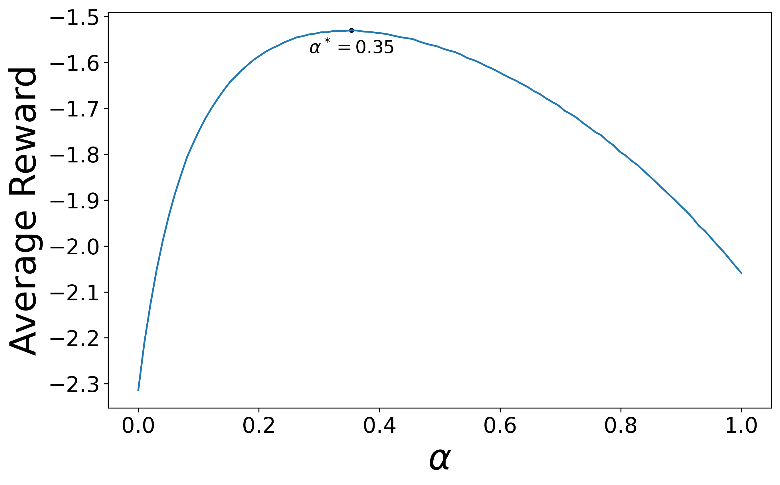
(a) Average reward as a function of stepsize $\alpha$, averaged over $10^{4}$ time steps and $10^{3}$ trials.

(b) The LMS agent with optimal stepsize ($\alpha=0.35$) tracks the latent scalar process well.

Figure 2: Tracking a latent scalar process using the LMS algorithm. The plots are generated with $\mu_{0}=0$, $\Sigma_{0}=1$, $\eta=0.9$, $\zeta=0.5$, and $\sigma=1$.

2.3.2 Exploration

In Example 3, actions do not impact observations. The following agent updates parameters in a similar incremental manner but then uses them to select actions that determine what information is revealed through observations.

Example 4.

(nonstationary Gaussian Thompson sampling) This agent interfaces with a finite action set $\mathcal{A}$ and real-valued observations $\mathcal{O}=\mathbb{R}$. The reward is taken to be the observation, so that $R_{t+1}=r(H_{t},A_{t},O_{t+1})=O_{t+1}$. Initialized with $\mu_{0}\in\mathbb{R}^{\mathcal{A}}$, the agent updates parameters according to

$$\mu_{t+1,a}=\left\{\begin{array}[]{ll}\eta\mu_{t,a}+\alpha_{t+1}(O_{t+1}-\eta\mu_{t,a})&\qquad\mathrm{if\ }a=A_{t}\\ \eta\mu_{t,a}&\qquad\mathrm{otherwise.}\end{array}\right.$$

Note that each observation only impacts the component of $\mu_{t}$ indexed by the executed action. The stepsize varies with time according to $\alpha_{t+1}=\Sigma_{t+1,A_{t}}/\sigma^{2}$, for a sequence initialized with a vector $\Sigma_{0}\in\mathbb{R}_{+}^{\mathcal{A}}$ and updated according to

$$\Sigma_{t+1,a}=\left\{\begin{array}[]{ll}\frac{1}{\frac{1}{\eta^{2}\Sigma_{t,a}+\zeta^{2}}+\frac{1}{\sigma^{2}}}&\qquad\mathrm{if\ }a=A_{t}\\ \eta^{2}\Sigma_{t,a}+\zeta^{2}&\qquad\mathrm{otherwise,}\end{array}\right.$$

where $\eta\in\mathbb{R}$, $\zeta\in\mathbb{R}_{+}$, $\sigma\in\mathbb{R}_{+}$ are scalar hyperparameters. Each $\hat{\theta}_{t,a}$ is drawn independently from $\mathcal{N}(\mu_{t,a},\Sigma_{t,a})$. Then, $A_{t}$ is sampled uniformly from the set $\operatorname*{arg\,max}_{a\in\mathcal{A}}\hat{\theta}_{t,a}$.

This agent is especially suited for a particular environment, which is characterized by latent random variables $\theta_{a}$, each independent and initially distributed $\mathcal{N}(\mu_{0,a},\Sigma_{0,a})$. Rewards and observations are generated according to $R_{t+1}=O_{t+1}=\theta_{A_{t}}+W_{t+1}$, with each $W_{t+1}$ sampled independently from $\mathcal{N}(0,\sigma^{2})$. It is natural to think of this as a stationary environment because the latent mean rewards $\theta_{a}$ do not change over time.

The environment we have described constitutes a bandit; this is a somewhat antiquated reference to a slot machine, which tends to “rob” players of their money. With multiple arms, as illustrated in Figure 3, a player chooses at each time an arm $A_{t}$ and receives a payout $R_{t+1}$. Because payout distributions are not listed, the player can learn them only by experimenting. As the gambler learns about each arm’s payouts, they face a dilemma: in the immediate future they expect to earn more by exploiting arms that yielded high payouts in the past, but by continuing to explore alternative arms they may learn how to earn higher payouts in the future.

Figure 3: A two-armed bandit.

In the stationary environment we have described, the distribution for arm $a$ is Gaussian with unknown mean $\theta_{a}$, which can be learned by observing payouts. For this environment, if $\eta=1$ and $\zeta=0$, the agent can be interpreted as selecting actions via Thompson sampling [Russo et al., 2018, Thompson, 1933]. In particular, at each time $t$, the posterior distribution of $\theta_{a}$ is $\mathcal{N}(\mu_{t,a},\Sigma_{t,a})$, and the agent samples statistically plausible estimates $\hat{\theta}_{t,a}$ from this distribution, then executes an action that maximizes among them.

If $\eta\in(-1,1)$ and $\zeta>0$, on the other hand, the environment is considered a nonstationary bandit because the arm payout distributions vary over time. In particular, the environment is characterized by latent random variables updated according to $\theta_{t+1,a}=\eta\theta_{t,a}+Z_{t+1,a}$, with each $Z_{t+1,a}$ independently sampled from $\mathcal{N}(0,\zeta^{2})$. The agent maintains parameters of the posterior distribution of $\theta_{t,a}$, which is $\mathcal{N}(\mu_{t,a},\Sigma_{t,a})$. For each action $a$, the agent samples $\hat{\theta}_{t,a}$ from the posterior distribution. The agent then executes an action that maximizes among these samples.

This nonstationary Gaussian Thompson sampling agent may be applied in other environments as well, whether or not observations are driven by Gaussian processes. For example, with a suitable choice of $\zeta$, it may exhibit reasonable behavior in the coin swapping environment of Example 2. However, the agent does not adequately address environments in which actions induce delayed consequences.

2.3.3 Delayed Consequences

The agent of Example 4 maintains parameters $\mu_{t}$ that serve the prediction $\eta\mu_{t,A_{t}}$ of the expected immediate reward $R_{t+1}$. These predictions can guide the agent to select actions that earn high immediate reward. To learn from and manage delayed rewards, the Q-learning algorithm [Watkins, 1989] instead maintains predictions $Q(S_{t},A_{t})$ of the expected discounted return $\sum_{k=0}^{\infty}\gamma^{k}R_{t+k+1}$. In addition to the action $A_{t}$, such predictions are conditioned on a situational state $S_{t}$, which provides context for the agent’s decision. The following example elaborates.

Example 5.

(optimistic Q-learning) This agent is designed to interface with any observation set $\mathcal{O}$ and any finite action set $\mathcal{A}$. It maintains an action value function $Q_{t}$, which maps the situational state $S_{t}$, which takes values in a finite sets $\mathcal{S}$, and action $A_{t}$ to a real value $Q_{t}(S_{t},A_{t})$. The situational state $S_{t}$ represents features of the history $H_{t}$ that are predictive of future value. It is determined by an update function $f$, which forms part of the agent design, according to

$$S_{t+1}=f(S_{t},A_{t},O_{t+1}),$$

and substitutes for history in the computation of rewards, which take the form $R_{t+1}=r(S_{t},A_{t},S_{t+1})$. We consider an optimistic version of Q-learning, which updates the action value function according to

$$Q_{t+1}(s,a)=\left\{\begin{array}[]{ll}Q_{t}(S_{t},A_{t})+\alpha\left(R_{t+1}+\gamma\max_{a\in\mathcal{A}}Q_{t}(S_{t+1},a)-Q_{t}(S_{t},A_{t})\right)+\zeta&\text{if }(s,a)=(S_{t},A_{t})\\ Q_{t}(s,a)+\zeta&\text{otherwise.}\end{array}\right.$$

Hyperparameters include a discount factor $\gamma\in(0,1)$, a stepsize $\alpha\in(0,1)$, and an optimistic boost $\zeta\in\mathbb{R}_{+}$. Each action $A_{t}$ is sampled uniformly from $\operatorname*{arg\,max}_{a\in\mathcal{A}}Q_{t}(S_{t},a)$.

To interpret this algorithm, consider situational state dynamics generated by a latent MDP, identified by a tuple $(\mathcal{S},\mathcal{A},r,P,S_{0})$. Here, $P$ is a random variable that specifies transition probabilities $P_{a,s,s^{\prime}}$ for actions $a\in\mathcal{A}$ and situational states $s,s^{\prime}\in\mathcal{S}$. In particular, $\mathbb{P}(S_{t+1}|P,A_{t},S_{t})=P_{A_{t},S_{t},S_{t+1}}$ for all $t$. If the hyperparameters $\gamma$, $\alpha$, and $\zeta$ anneal over time at suitable rates to $1$, $0$, and $0$, along the lines a more sophisticated version of Q-learning analyzed by Dong et al. [2022], the sequence $(Q_{t}:t\in\mathbb{Z}_{+})$ should converge to the optimal action value function of the MDP. By the same token, the agent would attain optimal average reward.

Versions of Q-learning permeate the RL literature. The one we have described presents some features that are worth discussing in relation to continual learning. First, action values are boosted by exploration bonuses, as considered by Sutton [1990], but in a manner that incentivizes visits to state-action pairs that have not been visited for a long time even if they have already been visited many times. Second, unlike common treatments that assume the aforementioned Markov property, our algorithm applies more broadly. It suffices for $S_{t}$ to enable useful predictions of value that guide effective decisions rather than approximate the state of the environment, which could be far more complex. This suits the spirit of continual learning, since the subject is oriented toward addressing very complex environments. Another noteworthy feature is that the hyperparameters $\gamma$, $\alpha$, and $\zeta$ are fixed. If the situational state dynamics were stationary, annealing hyperparameters over time is beneficial. However, as we will further discuss in Section 6.3, fixed parameters fare better in the face of nonstationarity.

2.3.4 Supervised Learning

Much of the literature on continual learning focuses on supervised learning (SL). As noted by Khetarpal et al. [2022], continual SL is a special case of reinforcement learning. In particular, take each observation to be a data pair $O_{t}=(Y_{t},X_{t})$, consisting of a label $Y_{t}$ assigned to the previous input $X_{t-1}$ and a next input $X_{t}$. Labels take values in a finite set $\mathcal{Y}$ and inputs take values in a set $\mathcal{X}$ which could be finite, countable, or uncountable. The set $\mathcal{O}$ of observations is a product $\mathcal{Y}\times\mathcal{X}$. Take each action $A_{t}$ to be a predictive distribution $P_{t}$, which assigns a probability $P_{t}(y)$ to each label $y\in\mathcal{Y}$. Hence, $P_{t}$ takes values in a unit simplex $\Delta_{\mathcal{Y}}$. We view $P_{t}$ as a prediction of the label $Y_{t+1}$ that will be assigned to the input $X_{t}$. The observation probability function $\rho$ samples the next data pair $O_{t+1}=(Y_{t+1},X_{t+1})$ in a manner that depends on history only through past observations, not past actions. Finally, take the reward function to be $r(H_{t},A_{t},O_{t+1})=\ln P_{t}(Y_{t})$. With this formulation, average reward is equivalent to average negative log-loss:

$$\overline{r}_{\pi}=\liminf_{T\rightarrow\infty}\mathbb{E}_{\pi}\left[\frac{1}{T}\sum_{t=0}^{T-1}\ln P_{t}(Y_{t+1})\right].$$ (2)

This is a common objective used in online supervised learning. The following agent is designed to minimize log-loss. Recall that $\Delta_{\mathcal{Y}}$ denotes the unit simplex or, equivalently, the set of probability vectors with one component per element of $\mathcal{Y}$.

Example 6.

(incremental deep learning) Consider an input space $\mathcal{X}$ and finite set of labels $\mathcal{Y}$. This agent is designed to interface with actions $\mathcal{A}=\Delta_{\mathcal{Y}}$ and observations $\mathcal{O}=\mathcal{Y}\times\mathcal{X}$. Consider a deep neural network with a softmax output node. The inference process maps an input $X_{t}$ to a predictive distribution $P_{t}(\cdot)=f_{\theta_{t}}(\cdot|X_{t})$. Here, $f$ is an abstract representation of the neural network and $\theta_{t}$ is the vector of parameters (weights and biases) at time $t$. Trained online via stochastic gradient descent (SGD) with a fixed stepsize to reduce log-loss, these parameters evolve according to

$$\theta_{t+1}=\theta_{t}+\alpha\nabla\ln f_{\theta_{t}}(Y_{t+1}|X_{t}).$$

This is a special case of our general reinforcement learning formulation, with action $A_{t}=P_{t}$, observation $O_{t+1}=(Y_{t+1},X_{t+1})$, and reward $r(H_{t},A_{t},O_{t+1})=\ln P_{t}(Y_{t+1})$.

Note that we could alternatively consider average accuracy as an objective by taking the action to be a label $A_{t}=\hat{Y}_{t+1}$. This label could be generated, for example, by sampling uniformly from $\operatorname*{arg\,max}_{y\in\mathcal{Y}}P_{t}(y)$. A reward function $r(H_{t},A_{t},O_{t+1})=\mathbbm{1}(Y_{t+1}=\hat{Y}_{t+1})$ can then be used to express accuracy. This is perhaps the objective most commonly used by applied deep learning researchers.

The incremental deep learning agent is designed for a prototypical supervised learning environment, where the relationship between inputs and labels is characterized by a random latent function $F$. In particular, $F\perp X_{0:t}$ and $\mathbb{P}(Y_{t+1}\in\cdot|F,H_{t})=F(\cdot|X_{t})$.

The agent can also be applied to a nonstationary supervised learning environment, where the latent function varies over time, taking the form of a stochastic process $(F_{t}:t\in\mathbb{Z}_{+})$. With this variation, $F_{t}\perp X_{0:t}$ and $\mathbb{P}(Y_{t+1}\in\cdot|F_{t},H_{t})=F_{t}(\cdot|X_{t})$. However, due to loss of plasticity, incremental deep learning does not perform as well in such an environment as one would hope [Dohare et al., 2021]. In particular, while the nonstationarity makes it important for the agent to continually learn, its ability to learn from new data degrades over time. A simple alternative addresses this limitation by periodically replacing the model under use with a new one, trained from scratch on recent data.

Example 7.

(model replacement) Given a neural network architecture and algorithm that trains the model on a fixed batch of $N$ data pairs, one can design a continual supervised learning agent as follows. At each time $t=0,\tau,2\tau,\ldots$, reinitialize the neural network parameters and train on $N$ most recent data pairs $(X_{t-n},Y_{t+1-n}:n=1,\ldots,N)$. No further training occurs until time $t+\tau$, when the model is reinitialized and retrained. Each prediction $A_{t}=P_{t}$ is given by $P_{t}(\cdot)=f_{\theta_{t}}(\cdot|X_{t})$, where $\theta_{t}$ is the most recent model. In particular, $\theta_{t+1}=\theta_{t}$ unless $t$ is a multiple of $\tau$. The hyperparameters $\tau$ and $N$ specify the replacement period and number of data pairs in each training batch.

This approach to continual learning is commonly used in production systems. For example, consider an agent that at the end of each $t$th day predicts the next day’s average electricity spot price $Y_{t+1}$. A prototypical system might, at the end of each month, initialize a neural network and train it on the preceding twelve months of data. Then, this model could be used over the subsequent month, at the end of which the next replacement arrives. The reason for periodically replacing the model is that very recent data is most representative of future price patterns, which evolve with the changing electricity market.

The reason for not replacing the model more frequently is the cost of training. There are a couple reasons for training only on recent history, in this case over the past twelve months. One is that recent data tends to best represent patterns that will recur in the future. However, this does not in itself prevent use of more data; given sufficient computation, it may be beneficial to train on all history, with data pairs suitably weighted to prioritize based on recency. The binding constraint is on computation, which scales with the amount of training data.

While model replacement is a common approach to continual learning, it is wasteful in and limited by its use of computational resources. In particular, each new model does not leverage computation invested in past models because it is trained from scratch. Developing an incremental training approach that affords a model benefits from all computation carried out since inception remains an important challenge to the field. Dohare et al. [2021] propose one approach. The subject remains an active area of research, motivated by limitations of the model replacement approach. These limitations also highlight the need for computational constraints in formulating a coherent objective for continual learning that incentivizes better agent designs.

2.4 Computational Constraints

Traditional machine learning paradigms such as supervised learning make use of fixed training datasets. A continual learning agent, on the other hand, processes endless data stream. An agent with bounded computational resources, regardless of scale, cannot afford to query every data point in its history $H_{t}$ at each time step because this dataset grows indefinitely. Instead, such an agent must act based on a more concise representation of historical information. In complex environments, this representation will generally forgo knowledge, some of which could have been used given greater computational resources. The notion that more compute ought to always be helpful in complex environments may be intuitively obvious. Nevertheless, it is worth pointing out corroboration by extensive empirical evidence from training large models on text corpi, where performance improves steadily along the range of feasible compute budgets [Brown et al., 2020, Hoffmann et al., 2022, Rae et al., 2022, Smith et al., 2022, Thoppilan et al., 2022].

In order to reflect the gating nature of computational resources in continual learning, we introduce a per-timestep computation constraint, as considered, for example, by Bagus et al. [2022], Lesort [2020], Prabhu et al. [2023b]. This specializes the continual learning problem formulation of Abel et al. [2023], which recognizes that constraints on the set of feasible agent policies give rise to continual learning behavior but does not focus on computation as the gating resource. As an objective for continual learning we propose maximization of average reward subject to this constraint on per-timestep computation. We believe that such a constraint is what gives rise to salient challenges of continual learning, such as catastrophic forgetting and loss of plasticity. Our theoretical analysis and empirical case studies will serve to motivate and justify this view.

Constraining per time step compute gives rise to our formulation of computation-constrained reinforcement learning:

$$\begin{split}\max_{\pi}&\quad\overline{r}_{\pi}\\ \text{s.t.}&\quad\text{computational constraint}.\end{split}$$ (3)

The nature of practical computational constraints and which is binding vary with prevailing technology and agent designs. For example, if calculations are carried out in parallel across an ample number of processors, it could be the channels for communication among them pose a binding constraint on overall computation. Or if agents are designed to use a very large amount of computer memory, that can become the binding constraint. Rather than study the capabilities of contemporary computer technologies to accurately identify current constraints, our above formulation intentionally leaves the constraint ambiguous. For the purposes of theoretical analysis and case studies presented in the remainder of the paper, we will usually assume all computation is carried out on a single processor that can execute a fixed number of serial floating point operations per time step, and that this is the binding constraint. We believe that insights generated under this assumption will largely carry over to formulations involving other forms of computational constraints.

While maximizing average reward subject to a computation constraint offers a coherent objective, an exact solution even for simple, let alone complex, environments is likely to be intractable. Nevertheless, a coherent objective is valuable for assessing and comparing alternative agent designs. Indeed, algorithmic ingredients often embedded in RL agents, such as Q-learning, neural networks, SGD, and exploration schemes such as optimism and Thompson sampling are helpful because they enable a favorable tradeoff between average reward and computation. Further, these ideas are scalable in the sense that they can leverage greater computational resources when available. As Sutton [2019] argues, with steady advances in computer technology, agent designs that naturally improve due to these advances will stand the test of time, while those that do not will phase out.

2.5 Learning Complex Skills over a Long Lifetime

An aspiration of continual learning is to design agents that exhibit ever more complex skills, building on skills already developed [Ring, 1994]. As opposed to paradigms that learn from a fixed data set, this aspiration is motivated by the continual growth of the agent’s historical data set, and thus, information available to the agent. With this perspective, continual learning researchers often ask whether specific design ingredients are really needed or if they should be supplanted by superior skills that the agent can eventually learn. For example, should an agent implement a hard-coded exploration scheme or learn to explore? Or ought an agent apply SGD to update its parameters rather than learn its own adaptation algorithm?

More concretely, consider the agent of Example 6, which implements SGD with a fixed stepsize. The performance of such an agent may improve with a stepsize adaptation scheme such as incremental delta-bar-delta (IDBD), which produces stepsizes that vary across parameters and time [Sutton, 1992]. With such a stepsize adaptation scheme, the agent can be seen as learning how to learn more effectively than fixed stepsize SGD. However, IDBD requires maintaining and updating three times as many parameters, and thus, increased compute. If compute were not a constraint, one could take things even further and design a more complex update procedure that requires not only computing gradients but also Hessians. For neural networks of practical scale, the associated computational requirements would be egregious.

As our discussion of two alternative to fixed stepsize SGD suggests, there is always room to improve average reward by designing the agent to learn more sophisticated skills. However, as we will discuss in the next section, this complexity is constrained by the agent’s information capacity, which is gated by computational constraints. There are always multiple ways to invest this capacity. For example, instead of maintaining statistics required by a stepsize adaptation scheme, a designer could increase the size of the neural network, which might also increase average reward.

Related to this is the stability-plasticity dilemma [McCloskey and Cohen, 1989, Ratcliff, 1990], a prominent subject in the continual learning literature. Stability is the resilience to forgetting useful skills, while plasticity is the ability to acquire new skills. Empirical studies demonstrate that agents do forget and that, as skills accumulate, become less effective at acquiring new skills [Dohare et al., 2021, Goodfellow et al., 2013, Kirkpatrick et al., 2017, Lesort, 2020]. Researchers have worked toward agent designs that improve stability and plasticity. But limited information capacity poses a fundamental tradeoff. For example, Mirzadeh et al. [2022] and Dohare et al. [2021] demonstrate that larger neural networks forget less and maintain greater plasticity. And as we will further discuss in Section 5, in complex environments, constrained agents must forget and/or lose plasticity, with improvements along one dimension coming at a cost to the other.

Summary

• An environment is characterized by a tuple $(\mathcal{A},\mathcal{O},\rho)$, comprised of a set of actions, a set of observations, and an observation probability function.

• The agent’s experience through time $t$ forms a history $H_{t}=(A_{0},O_{1},\ldots,A_{t-1},O_{t})$.

• Observations are generated as though

  $$O_{t+1}\sim\rho(\cdot|H_{t},A_{t}).$$

• The behavior of an agent is characterized by an agent policy $\pi$. Actions are generated as though

  $$A_{t}\sim\pi(\cdot|H_{t}).$$

• The designer’s preferences are encoded in terms of a reward function $r$, which generates rewards

  $$R_{t+1}=r(H_{t},A_{t},O_{t+1}).$$

• The average reward attained by an agent policy $\pi$ in an environment $(\mathcal{A},\mathcal{O},\rho)$ is

  $$\overline{r}_{\pi}=\liminf_{T\rightarrow\infty}\mathbb{E}_{\pi}\left[\frac{1}{T}\sum_{t=0}^{\infty}R_{t+1}\right].$$

• Design of a continual learning agent can be framed as maximizing average reward subject to a per-timestep computational constraint:

  $$\begin{split}\max_{\pi}&\quad\overline{r}_{\pi}\\ \text{s.t.}&\quad\text{computational constraint}.\end{split}$$

• Continual supervised learning with log-loss is a special case in which

  • $\mathcal{O}=\mathcal{X}\times\mathcal{Y}$, where $\mathcal{X}$ and $\mathcal{Y}$ are input and label sets,

  • $\mathcal{A}=\Delta_{\mathcal{Y}}$ is the unit simplex of predictive distributions,

  • each observation is a pair $O_{t+1}=(Y_{t+1},X_{t+1})$ comprising a label assigned to the previous input $X_{t}$ and the next input $X_{t+1}$,

  • the observation distribution $\rho(\cdot|H_{t},A_{t})$ depends on $(H_{t},A_{t})$ only through past observations $O_{1:t}$,

  • the reward function expresses the negative log-loss $R_{t+1}=\ln P_{t}(Y_{t+1})$.

  Another common reward function used in supervised learning expresses the accuracy $R_{t+1}=\mathbbm{1}(Y_{t+1}=\hat{Y}_{t+1})$, where the action is a label $A_{t}=\hat{Y}_{t+1}$.

3 Agent State and Information Capacity

Practical agent designs typically maintain a bounded summary of history, which we refer to as the agent state and which is used to select actions. Information encoded in the agent state is constrained to regulate computational requirements. In this section, we formalize these concepts in information-theoretic terms, along the lines of Jeon et al. [2023], Lu et al. [2021], and explore their relation to agent performance. The tools we develop allow us to more clearly distinguish continual from convergent learning and define and analyze stability and plasticity, as we do in Sections 4 and 5.

3.1 Agent State

Computational constraints prevent an agent from processing every element of history at each time step because the dataset grows indefinitely. To leverage more information than can be efficiently accessed from history, the agent needs to maintain a representation of knowledge that enables efficient computation of its next action. In particular, the agent must implement a policy $\pi$ that depends on a statistic $U_{t}$ derived from $H_{t}$, rather than directly on $H_{t}$ itself. Such a policy samples each action according to

$$A_{t}\sim\pi(\cdot|U_{t}).$$

The statistic $U_{t}$ must itself be computed using budgeted resources. An agent that computes $U_{t}$ directly from $H_{t}$ would run into constraints of the same sort that motivated construction of agent state in the first place. In particular, the agent cannot accesses all history within a time step and must maintain an agent state that facilitates efficient computation of the next agent state. To this end, $U_{t}$ serves two purposes: computation of $A_{t}$ and $U_{t+1}$. Specifically, there must be an update function $\psi$ such that

$$U_{t+1}\sim\psi(\cdot|U_{t},A_{t},O_{t+1}).$$

This sort of incremental updating allows $U_{t+1}$ to selectively encode historical information while amortizing computation across time. Since $U_{t}$ includes all information about $H_{t}$ that the agent will subsequently use, it can be thought of as a state; thus the term agent state.

Agents presented in Section 2.3 each use a highly compressed representation of history as agent state. In the scalar LMS algorithm of Example 3, the agent state $U_{t}=\mu_{t}$ is an estimate of a latent variable $\theta_{t}$. The agent state $U_{t}=(\mu_{t,a},\Sigma_{t,a}:a\in\mathcal{A})$ of Example 4 includes mean and variance estimates for each action. The optimistic Q-learning agent (Example 5) maintains a situational state and action value function as its agent state $U_{t}=(S_{t},Q_{t})$. Finally, with supervised deep learning, as described in Example 6, the agent state $U_{t}=(X_{t},\theta_{t})$ includes the current input and a vector of neural network parameters. If the agent were also to maintain a replay buffer $B_{t}$ of recent action-observation pairs for supplemental training, the replay buffer would also reside within the agent state $U_{t}=(X_{t},\theta_{t},B_{t})$. In each of these examples, the agent state is updated incrementally according to $U_{t+1}\sim\psi(\cdot|U_{t},A_{t},O_{t+1})$ for some function $\psi$.

3.2 Information Content

Intuitively, the agent state retains information from history to select actions and update itself. But how ought this information be quantified? In this section, we offer a formal approach based on information theory [Shannon, 1948]. Attributing precise meaning to information affords coherent characterization and analysis of information retained by an agent as well as forgetting and plasticity, which are subjects we will discuss in subsequent sections.

The agent state $U_{t}$ is a random variable since it depends on other random variables, including the agent’s experience $H_{t}$ through that time and possible algorithmic randomness arising in sampling from $\psi(\cdot|U_{t-1},A_{t-1},O_{t})$. A simple way of quantifying the information content of $U_{t}$ is in terms of the minimal number of bits that suffices for a lossless encoding. Or, using a unit of measurement more convenient for analysis of machine learning, the number of nats; there are $\ln 2$ nats per bit.

For reasons we will discuss, at large scale in terms of environment complexity and model size, this number ought to be well-approximated by the entropy $\mathbb{H}(U_{t})$. The entropy of a random variable $B$ with countable range is defined by

$$\mathbb{H}(B)=\mathbb{E}[-\ln\mathbb{P}(B)].$$

More generally, if the range is uncountable then entropy is defined by $\mathbb{H}(B)=\sup_{f\in\mathcal{F}_{\mathrm{finite}}}\mathbb{H}(f(B))$, where $\mathcal{F}_{\mathrm{finite}}$ is the set of functions that map $\mathcal{U}$ to a finite range.

Let us now discuss conditions under and the sense in which entropy closely approximates the number of nats that suffices for a lossless encoding. Consider a fixed environment and an agent design that is indexed by a parameter $M\in\mathbb{Z}_{++}$, with memory requirements that increase with $M$. Suppose that, for each $M$, the agent state $U_{t,1:M}$ is a vector with $M$ components. Further, suppose that these components are the first $M$ elements of a stationary stochastic process $(U_{t,m}:m\in\mathbb{Z}_{++})$. Under this assumption, $\mathbb{H}(U_{t,1:M})=\Theta(M)$. As a simple example, $(U_{t,m}:m\in\mathbb{Z}_{++})$ could be an iid sequence, with each $U_{t,m}$ representing a feature extracted from the history $H_{t}$. If these features are ordered from most to least important for selecting effective actions, it is natural to retain only the first $M$ in the agent state if that exhausts the memory budget. A standard result in information theory implies that, for any $\epsilon>0$, there is a $\mathbb{H}(U_{t,1:M})+\epsilon M$ nat encoding that affords lossless recovery of $U_{t,1:M}$ with a probability that approaches one as $M$ grows [Cover and Thomas, 2012, Theorem 5.4.2]. Hence, as $M$ grows, the percentage difference between $\mathbb{H}(U_{t,1:M})$ and the required number of nats vanishes.

The preceding argument assumed the agent state $U_{t}$ to be a high-dimensional vector with components generated by a stationary stochastic process. While this is not typically the case, we expect the key insight – that $\mathbb{H}(U_{t})$ closely approximates, in percentage terms, the number of nats that suffices for lossless encoding – to extend broadly to contexts where the agent state is a large object and the environment is much more complex, even than that. Intuitively and loosely speaking, this insight applies when the information encoded in $U_{t}$ originates from many independent random sources. A complex environment ought to afford an enormous diversity of random sources, and a large agent state ought to encode information from a large number. It is exactly such contexts that motivate the subject of continual learning.

3.3 Information Capacity

Recall our continual learning objective:

$$\max_{\pi} \quad\overline{r}_{\pi}$$

s.t. $$\quad\text{computational constraint}.$$

The nature of the computational constraint was purposely left ambiguous. If computer memory is binding, that directly constrains information content. We will assume for the remainder of this paper that the binding constraint is the number of floating point operations that can be carried out per time step (FLOPS). This does not necessarily constrain information content. For example, even if we take the agent state to be $U_{t}=H_{t}$ and the entropy $\mathbb{H}(U_{t})$ grows indefinitely, an agent can efficiently select each action based on sparsely queried data, perhaps by randomly sampling a small number of action-observation pairs from history. However, as a practical matter, common agent designs apply computation in ways that limit the amount of information that the agent retains. We refer to the constraint on information content of agent state as the information capacity.

A constraint on FLOPS limits information content when an agent is designed so that computation grows with information capacity. Supervised deep learning, as described in Example 6, offers a concrete case. Recall that, over each $t$th time step, the agent carries out a single SGD step:

$$\theta_{t+1}=\theta_{t}+\alpha\nabla\ln f_{\theta_{t}}(Y_{t+1}|X_{t}).$$

Each data pair $(X_{t},Y_{t+1})$ is immediately processed when observed, then discarded. Compute per data pair grows proportionally with the number of model parameters. Hence, a computation constraint restricts the number of model parameters. Conversely, the number of model parameters determines per-timestep computation. If each parameter is encoded by $K$ nats, a neural network model with $N$ parameters can encode $NK$ nats of information. We refer to this as the physical capacity of the neural network.

While information content is constrained not to exceed the physical capacity, large neural networks trained via SGD actually use only a fraction of their physical capacity to retain information garnered from data. Much of the $NK$ nats instead serves to facilitate computation. Therefore, the physical capacity constrains the information capacity to far fewer nats: $\mathbb{H}(U_{t})\ll NK$.

Similar reasoning applies if the agent state is expanded to include a replay buffer. In this case, the physical capacity is $NK+B$ nats, if $B$ nats are used to store the replay buffer. Again, the information capacity is constrained to far fewer nats than the physical capacity. As before only a fraction of the neural network’s physical capacity stores information content. But also, a replay buffer that stores raw data from history can typically be compressed losslessly to occupy a much smaller number of nats.

3.4 Performance versus Information Capacity

If the agent makes efficient use of its information capacity, it is natural to expect agent performance to increase as this constraint is loosened. Information theory offers an elegant interpretation of this relation. To illustrate this, let us work through this interpretation for the case of continual SL.

3.4.1 Prediction Error

Recall that, in our continual SL formulation, the agent’s action is a predictive distribution $A_{t}=P_{t}$ and the reward is taken to be $r(H_{t},A_{t},O_{t+1})=\ln P_{t}(Y_{t+1})$. Hence, the objective is to minimize average log-loss. To enable an elegant analysis, we define a prediction

$$P^{*}_{t}=\mathbb{P}(Y_{t+1}=\cdot|H_{t})=\operatorname*{arg\,max}_{Q\in\Delta_{\mathcal{Y}}}\mathbb{E}[\ln Q(Y_{t+1})|H_{t}]$$ (4)

as a gold standard. The expected reward $\mathbb{E}[\ln P^{*}_{t}(Y_{t+1})|H_{t}]$ represents the largest that a computationally unconstrained agent can attain given the history $H_{t}$. The difference between this gold standard value and the expected reward attained by the agent is expressed by the KL-divergence:

$${\mathbf{d}}_{\rm KL}(P^{*}_{t}\|P_{t})=\sum_{y\in\mathcal{Y}}P^{*}_{t}(y)\ln\frac{P^{*}_{t}(y)}{P_{t}(y)}=\mathbb{E}[\ln P^{*}_{t}(Y_{t+1})-\ln P_{t}(Y_{t+1})|H_{t}].$$

This KL-divergence serves as a measure of error between the agent’s prediction $P_{t}$ and the gold standard $P^{*}_{t}$. Maximizing average reward is equivalent to minimizing this prediction error, since

$$\underbrace{\mathbb{E}[\ln P_{t}(Y_{t+1})]}_{\text{reward}}=\underbrace{\mathbb{E}[\ln P^{*}_{t}(Y_{t+1})]}_{\text{optimal reward}}-\underbrace{\mathbb{E}[{\mathbf{d}}_{\rm KL}(P^{*}_{t}\|P_{t})]}_{\text{prediction error}}$$ (5)

and $\mathbb{E}[\ln P^{*}_{t}(Y_{t+1})]$ does not depend on $P_{t}$.

When making its prediction $P_{t}$, the agent only has information supplied by its agent state $U_{t}$. The best prediction that can be generated based on this information is

$$\tilde{P}_{t}=\mathbb{P}(Y_{t+1}=\cdot|U_{t})=\operatorname*{arg\,max}_{Q\in\Delta_{\mathcal{Y}}}\mathbb{E}[\ln Q(Y_{t+1})|U_{t}].$$ (6)

If the agent’s prediction $P_{t}$ differs from $\tilde{P}_{t}$, the error attained by the agent decomposes into informational versus inferential components, as established by the following result.

Theorem 1.

For all $t$,

$$\underbrace{\mathbb{E}[{\mathbf{d}}_{\rm KL}(P^{*}_{t}\|P_{t})]}_{\mathrm{prediction\ error}}=\underbrace{\mathbb{E}[{\mathbf{d}}_{\rm KL}(P^{*}_{t}\|\tilde{P}_{t})]}_{\mathrm{informational\ error}}+\underbrace{\mathbb{E}[{\mathbf{d}}_{\rm KL}(\tilde{P}_{t}\|P_{t})]}_{\mathrm{inferential\ error}}.$$

Proof.

For all $t$,

$$\mathbb{E}[{\mathbf{d}}_{\rm KL}(P^{*}_{t}\|P_{t})]= \mathbb{E}[\ln P^{*}_{t}(Y_{t+1})-\ln P_{t}(Y_{t+1})]$$

$$= \mathbb{E}[\mathbb{E}[\ln P^{*}_{t}(Y_{t+1})-\ln\tilde{P}_{t}(Y_{t+1})|H_{t}]]+\mathbb{E}[\mathbb{E}[\ln\tilde{P}_{t}(Y_{t+1})-\ln P_{t}(Y_{t+1})|U_{t}]]$$

$$= \mathbb{E}[{\mathbf{d}}_{\rm KL}(P^{*}_{t}\|\tilde{P}_{t})]+\mathbb{E}[{\mathbf{d}}_{\rm KL}(\tilde{P}_{t}\|P_{t})].$$

∎

3.4.2 Informational Error Quantifies Absent Information

The informational error can be interpreted as historical information absent from the agent state $U_{t}$ but that would be useful for predicting $Y_{t+1}$. This can be expressed in elegant information theoretic terms. To do so, we first review a few information measures for which Figure 4 illustrates intuitive relationships. Let $B$ and $C$ be random variables, and to simplify math, though the concepts extend to address uncountable ranges, let us assume for this discussion that each has countable range. The conditional entropy of $B$ conditioned on $C$ is defined by

$$\mathbb{H}(B|C)=\mathbb{E}\left[-\ln\mathbb{P}(B|C)\right].$$

It follows from the definition of conditional probability that $\mathbb{H}(B|C)=\mathbb{E}\left[-\ln\mathbb{P}(B,C)+\ln\mathbb{P}(C)\right]=\mathbb{H}(B,C)-\mathbb{H}(C)$. This represents the expected number of nats that remain to be revealed by $B$ after $C$ is observed, or the union of the two discs in the venn diagram minus the content of the blue disc. The mutual information between $B$ and $C$ is defined by

$$\mathbb{I}(B;C)=\mathbb{H}(B)-\mathbb{H}(B|C)=\mathbb{H}(C)-\mathbb{H}(C|B)=\mathbb{I}(C;B).$$

This represents the number of nats shared by $B$ and $C$, depicted as the intersection between the two discs. If the variables are independent then $\mathbb{I}(B;C)=0$. Finally, the mutual conditional information between $B$ and $C$, conditioned on a third random variable $D$, is defined by

$$\mathbb{I}(B;C|D)=\mathbb{I}(B;C,D)-I(B;D).$$

This represents information remaining in the intersection of $B$ and $C$ after $D$ is observed.

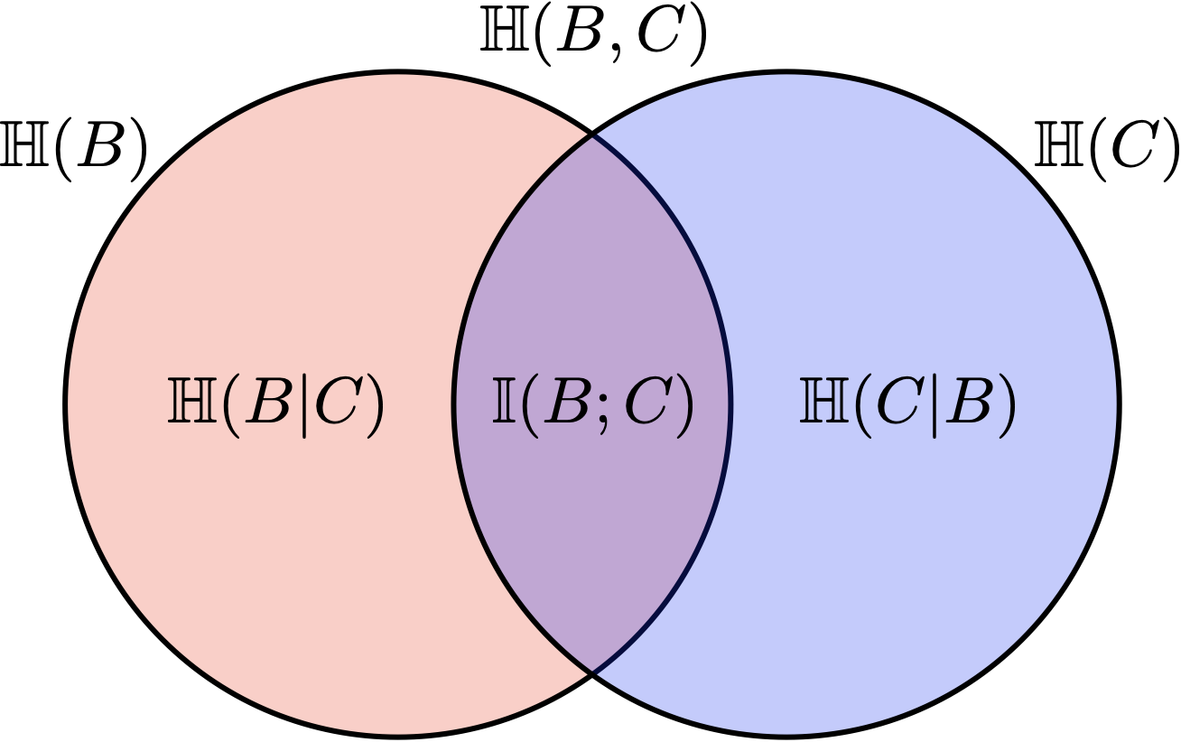
Figure 4: Venn diagram relating various information measures.

The following result establishes that the informational error $\mathbb{E}[{\mathbf{d}}_{\rm KL}(P^{*}_{t}\|\tilde{P}_{t})]$ equals the information $\mathbb{I}(Y_{t+1};H_{t}|U_{t})$ that the history $H_{t}$ presents about $Y_{t+1}$ but that is absent from $U_{t}$.

Theorem 2.

For all $t$,

$$\underbrace{\mathbb{E}[{\mathbf{d}}_{\rm KL}(P^{*}_{t}\|\tilde{P}_{t})]}_{\mathrm{informational\ error}}=\underbrace{\mathbb{I}(Y_{t+1};H_{t}|U_{t})}_{\mathrm{absent\ info}}.$$

Proof.

From the definitions of conditional entropy, $P^{*}_{t}$, and $\tilde{P}_{t}$, we have $\mathbb{H}(Y_{t+1}|H_{t})=\mathbb{E}[-\ln P^{*}_{t}(Y_{t+1})]$ and $\mathbb{H}(Y_{t+1}|U_{t})=\mathbb{E}[-\ln\tilde{P}_{t}(Y_{t+1})]$. It follows that,

$$\mathbb{E}[{\mathbf{d}}_{\rm KL}(P^{*}_{t}\|\tilde{P}_{t})]= \mathbb{E}[\ln P^{*}_{t}(Y_{t+1})-\ln\tilde{P}_{t}(Y_{t+1})]$$

$$= \mathbb{H}(Y_{t+1}|U_{t})-\mathbb{H}(Y_{t+1}|H_{t})$$

$$= \mathbb{H}(Y_{t+1}|U_{t})-\mathbb{H}(Y_{t+1}|U_{t},H_{t})$$

$$= \mathbb{I}(Y_{t+1};H_{t}|U_{t}).$$

The third equality follows from the fact that $Y_{t+1}\perp U_{t}|H_{t}$. ∎

3.4.3 Information Capacity Constrains Performance

It is natural to think that information capacity can constrain performance. This relationship is formalized by the following result.

Theorem 3.

For all $t$,

$$\underbrace{\mathbb{E}[{\mathbf{d}}_{\rm KL}(P^{*}_{t}\|P^{*}_{0})]}_{\mathrm{uninformed\ error}}-\underbrace{\mathbb{E}[{\mathbf{d}}_{\rm KL}(P^{*}_{t}\|\tilde{P}_{t})]}_{\mathrm{informational\ error}}=\underbrace{\mathbb{I}(Y_{t+1};U_{t})}_{\mathrm{useful\ info}}\leq\underbrace{\mathbb{H}(U_{t})}_{\mathrm{info}}.$$

Proof.

For all $t$,

$$\mathbb{E}[{\mathbf{d}}_{\rm KL}(P^{*}_{t}\|\tilde{P}_{t})]= \mathbb{I}(Y_{t+1};H_{t}|U_{t})$$

$$= \mathbb{I}(Y_{t+1};H_{t},U_{t})-\mathbb{I}(Y_{t+1};U_{t})$$

$$= \mathbb{I}(Y_{t+1};H_{t})-\mathbb{I}(Y_{t+1};U_{t})$$

$$= \mathbb{E}[{\mathbf{d}}_{\rm KL}(P^{*}_{t}\|P^{*}_{0})]-\mathbb{I}(Y_{t+1};U_{t}).$$

We arrive at the first inequality in our result by rearranging terms. The second follows from the fact that mutual information between two random variables is bounded by the entropy of each. ∎

Note that $P^{*}_{0}=\mathbb{P}(Y_{t+1}=\cdot|H_{0})=\mathbb{P}(Y_{t+1}=\cdot)$ is an uninformed prediction, which is based on no data. The left-hand-side expression $\mathbb{E}[{\mathbf{d}}_{\rm KL}(P^{*}_{t}\|P^{*}_{0})]-\mathbb{E}[{\mathbf{d}}_{\rm KL}(P^{*}_{t}\|\tilde{P}_{t})]$ is the reduction in informational error relative to an uninformed prediction. The middle expression $\mathbb{I}(Y_{t+1};U_{t})$ is the degree to which the agent state $U_{t}$ informs the agent about $Y_{t+1}$. The right-hand-side expression $\mathbb{H}(U_{t})$ is the information content of the agent state. If the information capacity constrains this content to be small, that in turn constrains the reduction in error. When the constraint is binding, larger information capacity affords smaller errors.

Summary

• An agent state $U_{t}$ is a summary of the history $H_{t}$ maintained to facilitate efficient computation of each action

  $$A_{t}\sim\pi(\cdot|U_{t}),$$

  and subsequent agent state

  $$U_{t+1}\sim\psi(\cdot|U_{t},A_{t},O_{t+1}).$$

  The agent policy of an agent designed in this way is characterized by the pair $(\psi,\pi)$.

• The information content of agent state is the number of nats required to encode it. At large scale and under plausible technical conditions, this is well-approximated by the entropy $\mathbb{H}(U_{t})$.

• An agent’s information capacity is a constraint on the information content and is typically limited by computational resources.

• Information capacity limits agent performance, which we measure in terms of average reward.

• In the special case of continual supervised learning with rewards $R_{t+1}=\ln P_{t}(Y_{t+1})$, expected reward is determined by prediction error via

  $$\underbrace{\mathbb{E}[\ln P_{t}(Y_{t+1})]}_{\text{reward}}=\underbrace{\mathbb{E}[\ln P^{*}_{t}(Y_{t+1})]}_{\text{optimal reward}}-\underbrace{\mathbb{E}[{\mathbf{d}}_{\rm KL}(P^{*}_{t}\|P_{t})]}_{\text{prediction error}},$$

  where $P_{t}$ denotes the agent’s prediction and $P_{t}^{*}(\cdot)=\mathbb{P}(Y_{t}=\cdot|H_{t})$ is the optimal prediction. Prediction error decomposes into informational and inferrential errors:

  $$\underbrace{\mathbb{E}[{\mathbf{d}}_{\rm KL}(P^{*}_{t}\|P_{t})]}_{\mathrm{prediction\ error}}=\underbrace{\mathbb{E}[{\mathbf{d}}_{\rm KL}(P^{*}_{t}\|\tilde{P}_{t})]}_{\mathrm{informational\ error}}+\underbrace{\mathbb{E}[{\mathbf{d}}_{\rm KL}(\tilde{P}_{t}\|P_{t})]}_{\mathrm{inferential\ error}},$$

  where $\tilde{P}_{t}(\cdot)=\mathbb{P}(Y_{t}=\cdot|U_{t})$ is the best prediction that can be produced based on the agent state. The informational error is equal to the information absent from agent state that would improve the prediction:

  $$\underbrace{\mathbb{E}[{\mathbf{d}}_{\rm KL}(P^{*}_{t}\|\tilde{P}_{t})]}_{\mathrm{informational\ error}}=\underbrace{\mathbb{I}(Y_{t+1};H_{t}|U_{t})}_{\mathrm{absent\ info}}.$$

  Informational error is limited by the information capacity according to

  $$\underbrace{\mathbb{E}[{\mathbf{d}}_{\rm KL}(P^{*}_{t}\|P^{*}_{0})]}_{\mathrm{uninformed\ error}}-\underbrace{\mathbb{E}[{\mathbf{d}}_{\rm KL}(P^{*}_{t}\|\tilde{P}_{t})]}_{\mathrm{informational\ error}}=\underbrace{\mathbb{I}(Y_{t+1};U_{t})}_{\mathrm{useful\ info}}\leq\underbrace{\mathbb{H}(U_{t})}_{\mathrm{info}}.$$

4 Vanishing-Regret Versus Continual Learning

Traditional framings of machine learning view the agent as accumulating knowledge about a fixed latent variable, which we refer to as a learning target. For example, in supervised learning, the learning target is typically taken to be a mapping from input to label probabilities. As a sanity check on agent performance, researchers then study regret relative to a hypothetical agent with privileged knowledge of the learning target. By the same token, traditional treatments of reinforcement learning center around learning about a latent MDP, or a derivative, such as a value function or a policy. Any of these can serve as a learning target, and again, regret analysis serves as a sanity check on agent performance.

Traditional framings orient agent designs toward ensuring that average regret vanishes as the dataset grows. To highlight this emphasis, we use the term vanishing-regret learning. Agents designed in this vein aim to reduce per-timestep regret, and are viewed as essentially “done” with learning when that becomes negligible.

Continual learning agents, on the other hand, engage in a perpetual mode of knowledge acquisition. Unlike vanishing-regret learning, the pace of continual learning does not taper off. Instead, in the never-ending process, some information is retained and some forgotten as new information is ingested. The notion of vanishing regret gives way to understanding this non-transient behavior.

In this section, we elaborate on this distinction between continual and vanishing-regret learning. To do so, we formalize the notion of a learning target and what it means for regret to vanish. We then discuss how computational constraints incentivize different qualitative behavior. The contrast offers insight into how and why continual learning agents should be designed differently. This discussion also leads us to reflect on why we have taken the environment $\mathcal{E}=(\mathcal{A},\mathcal{O},\rho)$ to be deterministic or, in other words, known, in contrast to work on vanishing-regret learning, which typically treats the environment as unknown.

4.1 Vanishing-Regret Learning

We begin by motivating the notation of a learning target and then discuss the role of vanishing regret in traditional machine learning. We leverage information theory as a lens that affords general yet simple interpretations of these concepts.

4.1.1 Learning Targets, Target Policies, and Vanishing Regret

Recall the coin tossing environment of Example 1. It is natural to think of an agent as learning about the coin biases from toss outcomes, with an eye toward settling on a simple policy that selects the coin with favorable bias. This framing can serve to guide comparisons among alternative agents and give rise to insight on how design decisions impact performance. For example, one could study whether each agent ultimately behaves as though it learned the coin biases. Such an analysis assesses agent performance relative to a benchmark, which is framed in terms of an agent with privileged knowledge of a learning target comprised of coin biases and a target policy that selects the favorable coin.

In the most abstract terms, a learning target is a random variable, which we will denote by $\chi$. A target policy $\tilde{\pi}$ assigns to each realization of $\chi$ a random policy. In particular, $\tilde{\pi}_{\chi}$ is a random variable that takes values in the set of policies. Intuitively, $\chi$ represents an interpretation of what an agent aims to learn about, and $\tilde{\pi}_{\chi}$ is the policy the agent would use if $\chi$ were known. Note that the target policy selects actions with privileged knowledge of the learning target. We will denote the average reward of the target policy conditioned on the learning target by

$$\overline{r}_{\chi,\tilde{\pi}}=\liminf_{T\rightarrow\infty}\mathbb{E}_{\tilde{\pi}_{\chi}}\left[\frac{1}{T}\sum_{t=0}^{T-1}R_{t+1}\Big{|}\chi\right],$$ (7)

where the subscript $\tilde{\pi}_{\chi}$ indicates the policy under which the conditional expectation is evaluated. Note that $\overline{r}_{\chi,\tilde{\pi}}$ is a random variable because it depends on $\chi$. This level of reward may be not attainable by any viable agent policy. This is because it can rely on knowledge of $\chi$, which the agent does not observe. An agent policy, on the other hand, generates each action $A_{t}$ based only on the history $H_{t}$. Rather than offer a viable agent policy, the learning target and target policy serve as conceptual tools that more loosely guide agent design and analysis.

For each duration $T\in\mathbb{Z}_{++}$, let

$$\overline{r}_{\pi,T}=\mathbb{E}_{\pi}\left[\frac{1}{T}\sum_{t=0}^{T-1}R_{t+1}\right]\qquad\text{and}\qquad\overline{r}_{\chi,\tilde{\pi},T}=\mathbb{E}_{\tilde{\pi}_{\chi}}\left[\frac{1}{T}\sum_{t=0}^{T-1}R_{t+1}\Big{|}\chi\right],$$

so that $\overline{r}_{\pi}=\liminf_{T\rightarrow\infty}\overline{r}_{\pi,T}$ and $\overline{r}_{\tilde{\pi},\chi}=\liminf_{T\rightarrow\infty}\overline{r}_{\chi,\tilde{\pi},T}$. Like $\overline{r}_{\chi,\tilde{\pi},T}$, the limit $\overline{r}_{\tilde{\pi},\chi}$ is a random variable. We define the average regret over duration $T$ incurred by $\pi$ with respect to $(\chi,\tilde{\pi})$ to be

$$\overline{\mathrm{Regret}}_{\chi,\tilde{\pi}}(T|\pi)=\mathbb{E}[\overline{r}_{\chi,\tilde{\pi},T}-\overline{r}_{\pi,T}].$$ (8)

This represents the expected per-timestep shortfall of the agent policy $\pi$ relative to the target policy $\tilde{\pi}_{\chi}$, which is afforded the advantage of knowledge about the learning target $\chi$.

We say $\pi$ exhibits vanishing regret with respect to $(\chi,\tilde{\pi})$ if $\limsup_{T\rightarrow\infty}\overline{\mathrm{Regret}}_{\chi,\tilde{\pi}}(T|\pi)\leq 0$. If rewards are bounded and limits of $\overline{r}_{\chi,\tilde{\pi},T}$ and $\overline{r}_{\pi,T}$ exist then, by the dominated convergence theorem, $\limsup_{T\rightarrow\infty}\mathbb{E}[\overline{r}_{\chi,\tilde{\pi},T}-\overline{r}_{\pi,T}]\leq\mathbb{E}[\overline{r}_{\chi,\pi}-\overline{r}_{\pi}]$, and therefore, vanishing regret is implied by $\mathbb{E}[\overline{r}_{\chi,\tilde{\pi}}-\overline{r}_{\pi}]\leq 0$. Intuitively, the notation of vanishing regret indicates that $\pi$ eventually performs at least as well as the target policy $\tilde{\pi}_{\chi}$ in spite of the latter’s privileged knowledge of $\chi$.

The choice of learning target and target policy are subjective in the sense that they are not uniquely determined by an agent-environment pair. Rather, they are chosen as means to interpret the agent’s performance in the environment. In particular, given $(\chi,\tilde{\pi})$, we can analyze how the agent learns about $\chi$ and uses that knowledge to make effective decisions. In this regard, three properties make for useful choices:

1. Given knowledge of the learning target $\chi$, an agent can execute $\tilde{\pi}_{\chi}$ in a computationally efficient manner.

2. The target policy $\tilde{\pi}_{\chi}$ attains a desired level of average reward.

3. An agent can learn enough about $\chi$ in reasonable time to perform about as well as $\tilde{\pi}_{\chi}$.

The first property ensures that knowledge of $\chi$ is actionable, and the second requires that resulting actions are performant to a desired degree. The third property ensures that acquiring useful knowledge about $\chi$ is feasible. These properties afford analysis of performance in terms of whether and how quickly an agent learns about $\chi$. We will further explore this sort of analysis in Section 4.1.2. But we close this section with a simple example of logit data and an agent that produces optimal predictions conditioned on history. This serves as an introduction to the notion of a learning target and what makes one useful.

Example 8.

(learning targets for logit data) Consider a binary observation sequence $(O_{t}:t\in\mathbb{Z}_{++})$ that is iid conditioned on a latent variable $\theta$. In particular, let $\mathcal{O}=\{0,1\}$, $\mathbb{P}(O_{t+1}=1|\theta,H_{t},A_{t})=e^{\theta}/(1+e^{\theta})$, and $\mathbb{P}(\theta\in\cdot)\sim\mathcal{N}(0,1)$. Each action is a predictive distribution $A_{t}=P_{t}$ and results in reward $R_{t+1}=\ln P_{t}(O_{t+1})$. We consider an optimal agent policy $\pi_{*}$, which generates predictive distributions $P^{*}_{t}\sim\pi_{*}(\cdot|H_{t})$ that perfectly condition on history: $P^{*}_{t}(\cdot)=\mathbb{P}(O_{t+1}=\cdot|H_{t})$. We will consider three different choices of learning target $\chi$ together, in each case, with the target policy $\tilde{\pi}_{\chi}$ that assigns all probability to $P_{t}^{\chi}=\mathbb{P}(O_{t+1}=\cdot|\chi,H_{t})$. This target policy executes actions that are optimally conditioned on knowledge of $\chi$ in addition to history.

For the “obvious” learning target $\chi=\theta$, $\overline{\mathrm{Regret}}_{\chi,\tilde{\pi}}(T|\pi)$ vanishes at a reasonable rate, which we will characterize in the next section. Intuitively, this is because, as data accumulates, the agent is able to produce estimates of $\theta$ that suffice for accurate predictions.

For contrast, let us now consider two poor choices of learning targets, each of which represents a different extreme. One is the “uninformative” learning target $\chi=\emptyset$, for which $\overline{r}_{\chi,\tilde{\pi},T}=\overline{r}_{\pi,T}$ for all $T$. Convergence is as fast as can be, and in fact, instant. However, the role of $\chi$ is vacuous. At the other extreme, suppose the learning target $\chi=(O_{t+1}:t\in\mathbb{Z}_{+})$ includes all observations from the past, present, and future. With this privileged knowledge, predictions $P^{\chi}_{t}(\cdot)=\mathbbm{1}(O_{t+1}=\cdot)$ perfectly anticipate observations. However, with this “overinformative” learning target, $\overline{\mathrm{Regret}}_{\chi,\tilde{\pi}}(T|\pi)$ does not vanish and instead converges to $\mathbb{E}[\ln(1+e^{-\theta})]>0$. This is because the agent never learns enough to compete with target policy, which has privileged access to future observations.

4.1.2 Regret Analysis

The machine learning literature offers a variety of mathematical tools for regret and sample complexity analysis. These tools typically study how agents accumulate information about a designated learning target and make decisions that become competitive with those that could be made with privileged knowledge of the learning target. To more concretely illustrate the nature of this analysis and the role of learning targets, we will present in this section examples of results in this area. In order to keep the exposition simple and transparent, we will restrict attention to supervised learning.

Rather than cover results about specific agents, we will review results about an optimal agent policy, which produces predictions $P^{*}_{t}(\cdot)=\mathbb{P}(Y_{t+1}=\cdot|H_{t})$. Such an agent maximizes $\mathbb{E}_{\pi}[\frac{1}{T}\sum_{t=0}^{T-1}R_{t+1}]$ over every duration $T$, with rewards given by $R_{t+1}=\ln P^{*}_{t}(Y_{t+1})$. Hence, the results we review pertain to what is possible rather than what is attained by a particular algorithm.

For any learning target $\chi$, we will take the target policy to be that which generates actions $P_{t}^{\chi}(y)=\mathbb{P}(Y_{t+1}=y|\chi,H_{t})$. This represents an optimal prediction for an agent with privileged knowledge of $\chi$ in addition to the history $H_{t}$. For this target policy, average regret satisfies

$$\overline{\mathrm{Regret}}_{\chi,\tilde{\pi}}(T|\pi)= \overline{r}_{\chi,\tilde{\pi},T}-\overline{r}_{\pi,T}$$

$$= \mathbb{E}\left[\mathbb{E}\left[\frac{1}{T}\sum_{t=0}^{T-1}\ln P^{\chi}_{t}(Y_{t+1})\Big{|}\chi\right]\right]-\mathbb{E}\left[\frac{1}{T}\sum_{t=0}^{T-1}\ln P^{*}_{t}(Y_{t+1})\right]$$

$$= \mathbb{E}\left[\frac{1}{T}\sum_{t=0}^{T-1}\mathbb{E}\left[\ln\frac{P^{\chi}_{t}(Y_{t+1})}{P^{*}_{t}(Y_{t+1})}\Big{|}\chi\right]\right]$$

$$= \mathbb{E}\left[\frac{1}{T}\sum_{t=0}^{T-1}{\mathbf{d}}_{\rm KL}(P_{t}^{\chi}\|P_{t}^{*})\right].$$

To characterize regret incurred by an optimal agent, we start with a basic result of [Jeon et al., 2023, Theorem 9]:

$$\overline{\mathrm{Regret}}_{\chi,\tilde{\pi}}(T|\pi)\leq\frac{\mathbb{H}(\chi)}{T}.$$ (9)

The right-hand side is the entropy of the learning target divided by the duration $T$. If this entropy is finite then, as $T$ grows, the right-hand side, and therefore regret, vanishes. That the bound increases with the entropy of the learning target is intuitive: if there is more to learn, regret ought to be larger for longer.

While the aforementioned regret bound offers useful insight, it becomes vacuous when the $\mathbb{H}(\chi)=\infty$. Entropy is typically infinite when $\chi$ is continuous-valued. In order to develop tools that enable analysis of continuous variables and that lead to much tighter bounds, even when $\mathbb{H}(\chi)<\infty$, let us introduce a new concept: the rate-distortion function. Let

$$\Theta_{\epsilon}=\left\{\tilde{\chi}:\mathbb{E}\left[{\mathbf{d}}_{\rm KL}\left(P_{t}^{\chi}\|P_{t}^{\tilde{\chi}}\right)\right]\leq\epsilon\text{ for all }t\right\}$$

be the set of all random variables $\tilde{\chi}$ that enable predictions close to those afforded by the $\chi$. The rate of $\chi$ with distortion tolerance $\epsilon$ is defined by the rate-distortion function:

$$\mathbb{H}_{\epsilon}(\chi)=\inf_{\tilde{\chi}\in\Theta_{\epsilon}}\mathbb{I}(\chi;\tilde{\chi}).$$ (10)

Loosely speaking, this is the number of nats required to identify a useful approximation to the learning target. The rate-distortion function $\mathbb{H}_{\epsilon}$ serves an alternative upper bound as well as a lower bound [Jeon et al., 2023, Theorem 12]:

$$\sup_{\epsilon\geq 0}\min\left(\frac{\mathbb{H}_{\epsilon}(\chi)}{T},\epsilon\right)\leq\overline{\mathrm{Regret}}_{\chi,\tilde{\pi}}(T|\pi)\leq\inf_{\epsilon\geq 0}\left(\frac{\mathbb{H}_{\epsilon}(\chi)}{T}+\epsilon\right).$$ (11)

Even when $\mathbb{H}(\chi)=\infty$, the rate $\mathbb{H}_{\epsilon}(\chi)$ can increase at a modest pace as $\epsilon$ vanishes. We build on Example 8 to offer a simple and concrete illustration. While that example was not framed as one of supervised learning, it can be viewed as such by taking each observation $O_{t+1}$ to encode only a label $Y_{t+1}$ resulting from a non-informative input $X_{t}$. We will characterize the rate-distortion function and regret for each of the three learning targets considered in Example 8.

Example 9.

(rate-distortion and convergence for logit data) Recall the environment of Example 8, in which binary labels are generated according to $\mathbb{P}(O_{t+1}=1|\theta,H_{t},A_{t})=e^{\theta}/(1+e^{\theta})$ based on a latent variable $\theta\sim\mathcal{N}(0,1)$.

For the “obvious” learning target $\chi=\theta$ and all $\tilde{\chi}$, $\mathbb{E}[{\mathbf{d}}_{\rm KL}(P^{\chi}_{t}\|P^{\tilde{\chi}}_{t})]\leq\mathbb{E}[(\chi-\mathbb{E}[\chi|\tilde{\chi}])^{2}]$. As a result, $\tilde{\chi}\sim\mathcal{N}(\chi,\epsilon)$ is an element of $\Theta_{\epsilon}$, and therefore,

$$\mathbb{H}_{\epsilon}(\chi)\leq\frac{1}{2}\ln\left(1+\frac{1}{\epsilon}\right).$$

It follows from Equation 11 that

$$\overline{\mathrm{Regret}}_{\chi,\tilde{\pi}}(T|\pi)\leq\ \inf_{\epsilon\geq 0}\left(\frac{1}{2T}\ln\left(1+\frac{1}{\epsilon}\right)+\epsilon\right)\ \leq\ \frac{\ln\left(1+2T\right)+1}{2T}.$$

For the “uninformative” learning target $\chi=\emptyset$, $\mathbb{H}_{\epsilon}(\chi)=0$, and therefore $\overline{\mathrm{Regret}}_{\chi,\tilde{\pi}}(T|\pi)=0$ for all $T$. For the “overinformative” learning target $\chi=(O_{t+1}:t\in\mathbb{Z}_{+})$, on the other hand, for $\epsilon<\mathbb{E}[\ln(1+e^{\theta})/(1+e^{\theta})]$, $\mathbb{H}_{\epsilon}(\chi)=\infty$ and $\overline{r}_{\chi,T}-\overline{r}_{*,T}>\mathbb{E}[\ln(1+e^{\theta})/(1+e^{\theta})]/2>0$.

For this example, though the “obvious” choice of learning target $\chi=\theta$ yields $\mathbb{H}(\chi)=\infty$, the rate $\mathbb{H}_{\epsilon}(\chi)$ is modest even for small positive values of $\epsilon$. Because of this, an optimal agent converges quickly, as expressed by $O((\ln T)/T)$ bound. Further, knowledge $\theta$ enables efficient computation of predictions $P_{t}(1)=\mathbb{P}(Y_{t+1}=1|\theta,H_{t})=e^{\theta}/(1+e^{\theta})$. On the other hand, the “underinformed” learning target $\chi=\emptyset$ is not helpful, and with respect to the “overinformed” learning target, regret does not vanish.

4.1.3 The Cosmic Learning Target

The universe is identified by a finite number of bits. Consider a “cosmic” learning target $\chi^{*}$ that expresses the entirety of this information. Lloyd [2002] derives an upper bound of $\mathbb{H}(\chi^{*})\leq 10^{120}$. For an agent that retains all information about $\chi^{*}$ that it observes, regret must vanish since, by Equation 9, $\overline{\mathrm{Regret}}_{\chi,\tilde{\pi}}(T|\pi)\leq\mathbb{H}(\chi^{*})/T$. However, this entropy is so large that the bound is effectively vacuous, establishing meaningful levels of error only for astronomically large $T$. The following example illustrates how a simpler learning target can give rise to a more relevant analysis.

Example 10.

(logit data from cosmic information) Consider again a supervised learning environment with binary labels, along the lines studied in Examples 8 and 9. In principle, given privileged knowledge of the cosmic learning target $\chi^{*}$, an agent should be able to generate perfect predictions $P^{\chi^{*}}_{t}(1)=\mathbb{P}(O_{t+1}=1|\chi^{*},H_{t},A_{t})=\mathbbm{1}(O_{t+1}=1)$. This is because all uncertainty is resolved by $\chi^{*}$. However, the rate at which $\overline{\mathrm{Regret}}_{\chi^{*},\tilde{\pi}}(T|\pi)$ vanishes may be too slow to be relevant.

Suppose that for some statistic $\theta$, which is determined by $\chi^{*}$, $\mathbb{P}(O_{t+1}=1|\theta,H_{t},A_{t})$ is very closely approximated by $e^{\theta}/(1+e^{\theta})$. Perhaps so closely that an agent with knowledge of $\theta$ will not be able to tell the difference over any reasonable time frame. Taking $\chi=\theta$ to be the learning target, we obtain the regret bound of Example 9.

A diligent reader may wonder how to reconcile the finiteness of cosmic information with infinite entropy of learning targets we sometimes consider, like in our treatment of logit data in Example 8. The continuous variable $\chi=\theta$ of that example, for which $\mathbb{H}(\theta)=\infty$, serves as an approximation. In particular, $\theta$ is a random variable with respect to a probability space $(\Omega,\mathbb{F},\mathbb{P})$ and thus determined by an atomic outcome $\omega$ in an infinite set $\Omega$. The infinite set approximates the set of possible realizations of the cosmic learning target $\chi^{*}$. In particular, the latter set is so large that, for practical purposes, we consider it infinite. This gives rise to a mathematical formalism that accommodates random variables with infinite entropy.

4.2 Continual Learning

Unlike more traditional framings of machine learning, continual learning does not generally afford an obvious choice of learning target. In traditional framings, the agent is considered “done” with learning when it has gathered enough information about a learning target to make effective decisions. Performant continual learning agents perpetually ingest new information. This unending process is incentivized by constraints, as we now discuss.

4.2.1 Constraints Induce Persistent Regret

Recall that practical agent designs typically maintain an agent state, with behavior characterized by functions $\psi$ and $\pi$. In particular, the agent state evolves according to $U_{t+1}\sim\psi(\cdot|U_{t},A_{t},O_{t+1})$ and actions are sampled according to $A_{t}\sim\pi(\cdot|U_{t})$. Hence, the agent policy is encoded in terms of the pair $(\psi,\pi)$. Let $\overline{r}_{\psi,\pi}=\mathbb{E}_{\pi,\psi}[\frac{1}{T}\sum_{t=0}^{T-1}R_{t+1}]$ denote the average reward attained by such an agent.

The information content of $U_{t}$ is quantified by the entropy $\mathbb{H}(U_{t})$, which is constrained by the agent’s information capacity. As discussed in Section 3.3, for common scalable agent designs, computation grows with this information content. Hence, computational constraints limit information capacity. To understand implications of this restriction, in this section, we focus on the problem of agent design with fixed information capacity $C$:

$$\begin{split}\max_{\psi,\pi}&\quad\overline{r}_{\psi,\pi}\\ \text{s.t.}&\quad\sup_{t}\mathbb{H}(U_{t})\leq C.\end{split}$$ (12)

The following simple example, which is similar to one presented in [Sutton et al., 2007, Section 2], illustrates how such a constraint induces persistent regret.

Example 11.

(bit flipping) Consider an environment that generates a sequence of binary observations $\mathcal{O}=\{0,1\}$, initialized with $O_{1}$ distributed $\mathrm{Bernoulli}(1/2)$, and evolving according to $\mathbb{P}(O_{t+1}=o|p,H_{t},A_{t})=p(1-o)+(1-p)o$, where $p$ is a random variable. Note that $p$ governs the probability of a bit flip. Each action is a binary prediction $A_{t}$ of the next observation $O_{t+1}$ and yields reward $R_{t+1}=\mathbbm{1}(A_{t}=O_{t+1})$. In other words, the agent predicts the next bit and receives a unit of reward if its prediction is correct.

It is natural to consider $\chi=p$ as a learning target. In particular, with privileged knowledge of this learning target, an agent can act according to a target policy $\tilde{\pi}$ that generates a prediction $A_{t}=1$ if and only if $\mathbb{P}(O_{t+1}=1|p,H_{t})>1/2$ or, equivalently, $p(1-O_{t})+(1-p)O_{t}>1/2$. The optimal unconstrained agent policy $\pi$ generates action $A_{t}=1$ if and only if $\mathbb{P}(O_{t+1}=1|H_{t})>1/2$ and satisfies $\overline{\mathrm{Regret}}_{\chi,\tilde{\pi}}(T|\pi)\rightarrow 0$. This is because, if not hindered by constraints, an agent can identify $p$ over time from observations.

Now suppose the agent is constrained by an information capacity of $C=\ln 2\mathrm{\ nats}=1\mathrm{\ bit}$. Encoding an accurate approximation of $p$ in the agent state becomes infeasible. Instead, the optimal solution to Equation 12 is comprised of an agent state update function $U_{t}=O_{t}$ and a policy function for which $A_{t}=1$ if and only if $\mathbb{E}[p](1-U_{t})+\mathbb{E}[1-p]U_{t}>1/2$. In other words, the agent simply retains its most recent observation as agent state and predicts a bit flip with probability $\mathbb{E}[p]$. This agent does not aim to identify $\chi=p$ nor, for that matter, any nontrivial learning target. And regret with respect to $\overline{\mathrm{Regret}}_{\chi,\tilde{\pi}}(T|\pi)$ does not vanish.

4.2.2 Nonstationary Learning Targets

Continual learning is often characterized as addressing nonstationary environments. But whether an environment is nonstationary is a subjective matter. With respect to the cosmic learning target $\chi^{*}$, any environment is stationary. However, as illustrated by Example 10, it can be useful to view an environment as nonstationary with respect to a simpler latent stochastic process $(\theta_{t}:t\in\mathbb{Z}_{++})$. An agent that tracks this process can be viewed at each time $t$ as trying to learn about $\theta_{t}$. This suggests viewing $\chi_{t}=\theta_{t}$ as a time-varying – or nonstationary – learning target.

Motivated by this view, we interpret nonstationarity as indicating agent behavior that is naturally explained by a time-varying learning target. Example 11 illustrates how this sort of behavior is incentivized by restricting information capacity. The optimal unconstrained agent learns about the latent variable $p$, which constitutes a fixed learning target. On the other hand, the capacity-constrained agent learns at each time about $O_{t}$. This bit of information is ingested into the agent state and can be viewed as a nonstationary learning target $\chi_{t}=O_{t}$.

Our narrative is aligned with that of Sutton et al. [2007], who suggest that tracking a nonstationary learning target is warranted even in a stationary environment if the environment is sufficiently complex. The cosmic learning target $\chi^{*}$ is helpful to making this point. Consider a supervised learning environment for which an enormous amount of information is required to attain reasonable performance. In other words, for any reasonable $\epsilon$, $\mathbb{H}_{\epsilon}(\chi^{*})$ is huge. An agent with modest capacity $C\ll\mathbb{H}_{\epsilon}(\chi^{*})$ ought not aim to accumulate all information required to attain error $\epsilon$ because of its insufficient information capacity. However, it may be possible to attain error $\epsilon$ by only retaining at each time step information that will be helpful in the near term. This amounts to tracking a nonstationary learning target.

Our notion of a nonstationary learning target relates to the work of Abel et al. [2023], which proposes a definition of continual reinforcement learning. This definition offers a formal expression of what it means for an agent to never stop learning. The characterization is subjective in that it defines non-convergence with respect to a basis, which is a fixed set of policies. An agent is interpreted as searching among these and then of converging if it settles on one that it follows thereafter. The work associates continual learning with non-convergence. A learning target offers an alternative subjective construct for interpretation of agent behavior. Loosely speaking, if an agent converges on an element of the basis, that can be thought of as deriving from a fixed learning target. Perpetually transitioning among element of the basis is akin to pursuing a nonstationary learning target.

4.3 On Learning About an Unknown Environment

In traditional framings of machine learning, it is common to characterize the environment as a random (unknown) latent variable. The agent is then interpreted as learning about the environment – that is, this random variable – from its experience. Indeed, the random environment can serve as a learning target in the vein of vanishing-regret learning. In supervised learning, if the input distribution is known, this latent variable may be the unknown function that maps inputs to distributions over labels. In some traditional framings of reinforcement learning, it may be the unknown transition probability matrix of a Markov Decision Process (MDP).

In contrast, our general formulation of continual learning, as described in Section 2.1, takes the environment, and in particular, the observation probability function $\rho$, to be known. With this formulation, the environment is no longer a random variable and can not serve as a useful learning target. In this subsection, we will motivate this decision. We first discuss why a deterministic characterization is general and minimal. We then explain that, because the sort of environment of interest to continual learning does not give rise to an obvious fixed learning target, random characterizations of the environment do not afford the kind of interpretation and analysis enjoyed by vanishing-regret learning.

As discussed in Section 2.1, the dynamics represented by a random observation probability function $\tilde{\rho}$ can be expressed in terms of a deterministic one $\rho$ for which $\rho(\cdot|H_{t},A_{t})=\mathbb{E}[\tilde{\rho}(\cdot|H_{t},A_{t})|H_{t},A_{t}]$. The converse also holds. In particular, for any deterministic $\rho$ and random variable $\chi$, we can define an equivalent random $\tilde{\rho}$ for which $\tilde{\rho}(\cdot|H_{t},A_{t})=\mathbb{P}(O_{t+1}\in\cdot|\chi,H_{t},A_{t})$. Note that $\tilde{\rho}$ offers an equivalent characterization because $\rho(\cdot|H_{t},A_{t})=\mathbb{P}(O_{t+1}\in\cdot|H_{t},A_{t})=\mathbb{E}[\mathbb{P}(O_{t+1}\in\cdot|\chi,H_{t},A_{t})|H_{t},A_{t}]=\mathbb{E}[\tilde{\rho}(\cdot|H_{t},A_{t})|H_{t},A_{t}]$. Since this is true for any random variable $\chi$, there are many random environments that represent the same deterministic environment. As such, the deterministic representation is minimal, while the random representation requires choice of a random variable $\chi$, which is inconsequential to the dynamics of the environment.

In the traditional framing of supervised learning, data pairs are assumed to be exchangeable. Consequently, de Finetti’s Theorem establishes existence of a learning target $\chi$ conditioned on which the data pairs are iid [de Finetti, 1929]. It is natural to think of $\chi$ as identifying an unknown environment and bringing to bear interpretation and analysis afforded by vanishing-regret learning. Specifically, assuming the input distribution is known, $\chi$ is often taken to be an unknown function that maps inputs to distributions over labels. A similar story goes for the traditional framing of reinforcement learning. Under a weaker exchangeability condition presented in Appendix A, it is natural to characterize dynamics in terms of an unknown MDP $\chi$. In both cases, an agent can learn over time to do about as well as if $\chi$ were known.

In contrast, environments of the sort considered in continual learning tend not to give rise to an obvious choice of fixed learning target. In particular, regret generally does not vanish with respect to any particular learning target that enables efficient computation of performant actions. For example, Liu et al. [2023a] discusses how regret does not vanish with respect to common choices of learning targets in non-stationary bandit learning. Absent the analytic role of a learning target, we opted for minimality in using a deterministic environment characterization for our formulation of continual learning. That being said, for the purpose of exposition, it can often be more intuitive to characterize a specific environment using a latent variable model. For instance, many of the examples in this monograph are described as latent AR(1) processes, such as the scalar tracking problem in Section 2.3.1. Such a characterization can be helpful to facilitate interpretation.

Summary

• A learning target (denoted by $\chi$) is random variable that represents what an agent aims to learn about.

• A target policy (denoted by $\tilde{\pi}_{\chi}$) is a random variable that takes values in the set of policies which represents the policy the agent would use if $\chi$ were known.

• For each duration $T\in\mathbb{Z}_{++}$,

  $$\overline{r}_{\pi,T}=\mathbb{E}_{\pi}\left[\frac{1}{T}\sum_{t=0}^{T-1}R_{t+1}\right]\qquad\text{and}\qquad\overline{r}_{\chi,\tilde{\pi},T}=\mathbb{E}_{\tilde{\pi}_{\chi}}\left[\frac{1}{T}\sum_{t=0}^{T-1}R_{t+1}\Big{|}\chi\right].$$

• The average regret over duration $T$ incurred by $\pi$ w.r.t $(\chi,\tilde{\pi})$ is

  $$\overline{\mathrm{Regret}}_{\chi,\tilde{\pi}}(T|\pi)=\mathbb{E}\left[\overline{r}_{\chi,\tilde{\pi},T}-\overline{r}_{\pi,T}\right].$$

• $\pi$ exhibits vanishing regret w.r.t. $(\chi,\tilde{\pi})$ if $\limsup_{T\to\infty}\overline{\mathrm{Regret}}_{\chi,\tilde{\pi}}(T|\pi)\leq 0$.

• In the special case of continual supervised learning, $P_{t}^{*}(y)=\mathbb{P}(Y_{t+1}=y|H_{t})$ maximizes $\overline{r}_{\pi,T}$ and $P_{t}^{\chi}(y)=\mathbb{P}(Y_{t+1}=y|\chi,H_{t})$ maximizes $\overline{r}_{\chi,\tilde{\pi},T}$ for every duration $T$ For the above optimal choices of $\pi,\tilde{\pi}_{\chi}$,

  $$\overline{\mathrm{Regret}}_{\chi,\tilde{\pi}}(T|\pi)=\mathbb{E}\left[\frac{1}{T}\sum_{t=0}^{T-1}{\mathbf{d}}_{\rm KL}(P_{t}^{\chi}\|P_{t}^{*})\right].$$

  For all durations $T$,

  $$\overline{\mathrm{Regret}}_{\chi,\tilde{\pi}}(T|\pi)\leq\frac{\mathbb{H}(\chi)}{T}.$$

  For continuous-valued $\chi$, $\mathbb{H}(\chi)$ is often $\infty$, leading to a vacuous upper bound. The bound can be improved via rate-distortion theory. For any $\epsilon\geq 0$, let

  $$\Theta_{\epsilon}=\left\{\tilde{\chi}:\mathbb{E}[{\mathbf{d}}_{\rm KL}(P_{t}^{\chi}\|P_{t}^{\tilde{\chi}})]\leq\epsilon\text{ for all }t\right\}$$

  be the set of all random variables $\tilde{\chi}$ which enable predictions with distortion at most $\epsilon$. The rate of $\chi$ with distortion tolerance $\epsilon$ is defined by the rate-distortion function:

  $$\mathbb{H}_{\epsilon}(\chi)=\inf_{\tilde{\chi}\in\Theta_{\epsilon}}\mathbb{I}(\chi;\tilde{\chi}).$$

  For all durations $T$,

  $$\sup_{\epsilon\geq 0}\min\left(\frac{\mathbb{H}_{\epsilon}(\chi)}{T},\epsilon\right)\leq\overline{\mathrm{Regret}}_{\chi,\tilde{\pi}}(T|\pi)\leq\inf_{\epsilon\geq 0}\left(\frac{\mathbb{H}_{\epsilon}(\chi)}{T}+\epsilon\right).$$

• The notion of learning about an uncertain environment does not play a central role in continual learning as it does in vanishing-regret learning:

  • In vanishing-regret learning, it is common to characterize the environment as a random (unknown) latent variable.

  • In contrast, our general formulation of continual learning takes the environment, and in particular, the observation probability function $\rho$, to be deterministic (known). This characterization is general and minimal.

  • In continual learning, random characterizations of the environment do not generally afford the kind of interpretation and analysis enjoyed by vanishing-regret learning. This is because performant agents do not generally focus on identifying a fixed learning target.

5 Stability Versus Plasticity

While the subjects of catastrophic forgetting and loss of plasticity have attracted a great deal of attention in the continual learning literature, the terms have lacked definitional clarity of the sort that would afford coherent reasoning about tradeoffs. Both notions relate to how an agent processes information. Catastrophic forgetting refers to elimination of useful information. Loss of plasticity refers to an inability to ingest useful new information. In this section, we build on information-theoretic tools introduced in the previous section to formalize these concepts and clarify the interaction between information capacity, stability, and plasticity. To keep the analysis simple, we restrict attention to the special case of continual supervised learning, as presented in Section 2.3.4. Recall that each action is a predictive distribution $A_{t}=P_{t}$ and each reward $R_{t+1}=\ln P_{t}(Y_{t+1})$ is the logarithm of the probability assigned to the realized label.

5.1 Stability-Plasticity Decomposition

If the agent had infinite information capacity and could maintain history as its agent state $U_{t}=H_{t}$ then the informational error would be $\mathbb{E}[{\mathbf{d}}_{\rm KL}(P^{*}_{t}\|\tilde{P}_{t})]=\mathbb{I}(Y_{t+1};H_{t}|H_{t})=0$. However, with an agent state that retains partial information, the error will typically be larger. In this way, and as expressed by Theorem 3, a constraint on capacity can induce error. This happens through requiring that the agent either forget some old information, forgo ingestion of some new information, or both.

We can formalize the relation between these quantities in information-theoretic terms. At each time step $t$, the informational error $\mathbb{E}[{\mathbf{d}}_{\rm KL}(P^{*}_{t}\|\tilde{P}_{t})]$ arises as a consequence of useful information forgotten or forgone due to implasticity over previous time steps. As shorthand, let $H_{t-k:t}=(O_{t-k},\ldots,O_{t})$. The error due to information forgotten $k$ time steps earlier can be expressed as $I(Y_{t+1};U_{t-k-1}|U_{t-k},H_{t-k:t})$: the information about $Y_{t+1}$ that is available in $U_{t-k-1}$ but not the next agent state $U_{t-k}$ or the subsequent experience $H_{t-k+1:t}$. In other words, this is the information lost in transitioning from $U_{t-k-1}$ to $U_{t-k}$ and not recoverable by time step $t$. The error due to implasticity $k$ time steps earlier can be expressed as $\mathbb{I}(Y_{t+1};O_{t-k}|U_{t-k},H_{t-k+1:t})$: the information about $Y_{t+1}$ that is available in $O_{t-k}$ but absent from the preceding agent state $U_{t-k}$ and the subsequent experience $H_{t-k+1:t}$. In other words, this is information presented by $O_{t-k}$ but not $U_{t-k}$ and that is not otherwise available through time step $t$.

The following theorem provides a formal decomposition, attributing error to forgetting and implasticity. Note that actions are omitted because in the case of supervised learning they do not impact observations.

Theorem 4.

For all $t\in\mathbb{Z}_{+}$,

$$\underbrace{\mathbb{E}[{\mathbf{d}}_{\rm KL}(P^{*}_{t}\|\tilde{P}_{t})]}_{\mathrm{error}}=\sum_{k=0}^{t}\left(\underbrace{\mathbb{I}(Y_{t+1};U_{t-k-1}|U_{t-k},H_{t-k:t})}_{\mathrm{forgetting\ at\ lag\ }k}+\underbrace{\mathbb{I}(Y_{t+1};O_{t-k}|U_{t-k},H_{t-k+1:t})}_{\mathrm{implasticity\ at\ lag\ }k}\right).$$

Proof.

We have

$$\mathbb{E}[{\mathbf{d}}_{\rm KL}(P^{*}_{t}\|\tilde{P}_{t})] \overset{(a)}{=}\mathbb{I}(Y_{t+1};H_{t}|U_{t})$$

$$\overset{(b)}{=}\mathbb{I}(Y_{t+1};H_{t},U_{0:t-1}|U_{t})$$

$$\overset{(c)}{=}\sum_{k=0}^{t}\mathbb{I}(Y_{t+1};O_{t-k},U_{t-k-1}|U_{t-k:t},H_{t-k+1:t})$$

$$\overset{(d)}{=}\sum_{k=0}^{t}\mathbb{I}(Y_{t+1};O_{t-k},U_{t-k-1}|U_{t-k},H_{t-k+1:t})$$

$$\overset{(e)}{=}\sum_{k=1}^{t}\left(\mathbb{I}(Y_{t+1};U_{t-k-1}|U_{t-k},H_{t-k:t})+\mathbb{I}(Y_{t+1};O_{t-k}|U_{t-k},H_{t-k+1:t})\right),$$

where $(a)$ follows from Theorem 2; $(b)$ follows from $U_{0:t-1}\perp Y_{t+1}|U_{t},H_{t}$; $(c)$ follows from the chain rule of mutual information, and we take $Y_{0}$ and $U_{-1}$ to be the singleton $\emptyset$; $(d)$ follows from the fact that for all $j$, $U_{j+1}$ is determined by $(U_{j},O_{j+1})$ and independent algorithmic randomness; and $(e)$ follows from chain rule of mutual information. ∎

Implasticity and forgetting terms are indexed by a lag $k$ relative to the current time step $t$. In the process of updating the agent state from $U_{t-k-1}$ to $U_{t-k}$ in response to an observation, information may be ingested and/or forgotten. The implasticity and forgetting terms measure how this ultimately impacts the agent’s ability to predict $Y_{t+1}$. Summing over lags $k$ produces the immediate error $\mathbb{I}(Y_{t+1};H_{t}|U_{t})$.

The implasticity at lag $k$ measures the amount of information presented by $O_{t-k}$ that is useful for predicting $Y_{t+1}$ that the agent fails to ingest and is absent from the intermediate data $H_{t-k+1:t}$. Note that, due to the conditioning on the data $H_{t-k+1:t}$, this term only penalizes the inability to extract information about $Y_{t+1}$ that will not be again available from observations between $t-k$ and $t$.

The forgetting at lag $k$ derives from the agent ejecting information that is relevant to predicting $Y_{t+1}$ when updating its agent state from $U_{t-k-1}$ to $U_{t-k}$. Again, due to conditioning on $H_{t-k:t}$, this term only penalizes for forgotten information that cannot be recovered from other observations to be made before time step $t$.

Our decomposition indicates that errors due to implasticity and forgetting are forward looking in the sense that they only impact predictions at subsequent times; thus the lag $k$ relative to prediction error. This is in contrast with much of the continual SL literature, which aims to develop agents that remember information that would have been useful in their past, even if that is unlikely to be useful to their future. Indeed, the term catastrophic forgetting typically refers to loss of useful information, whether useful in the future or past.

Our expressions for implasticity and forgetting are complicated by sums over lags. The expressions simplify greatly when the input sequence $X_{t}$ is independent of history, i.e., $X_{t+1}\perp H_{t}$, and when the sequence of agent states and observations forms a stationary stochastic process. This corresponds to a prototypical nonstationary supervised learning formulation: iid inputs and a mapping to label probabilities that is modulated by a stationary stochastic process.

Theorem 5.

Suppose $((U_{t},O_{t}):t\in\mathbb{Z}_{+})$ is a stationary process and, for all $t\in\mathbb{Z}_{+}$, $X_{t+1}\perp H_{t}$. Then, for all $t\in\mathbb{Z}_{+}$,

$$\lim_{t\to\infty}\underbrace{\mathbb{E}[{\mathbf{d}}_{\rm KL}(P^{*}_{t}\|\tilde{P}_{t})]}_{\mathrm{error}}=\lim_{t\to\infty}\left(\underbrace{\mathbb{I}(H_{t+1:\infty};U_{t-1}|U_{t},O_{t})}_{\mathrm{forgetting}}+\underbrace{\mathbb{I}(H_{t+1:\infty};O_{t}|U_{t})}_{\mathrm{implasticity}}\right).$$

Proof.

We establish the result by taking limits of the expressions from Theorem 4 for cumulative forgetting and implasticity. The forgetting term yields

$$\lim_{t\to\infty}\sum_{k=0}^{t}\mathbb{I}(Y_{t+1};U_{t-k-1}|U_{t-k},H_{t-k:t}) \overset{(a)}{=}\lim_{t\to\infty}\sum_{k=0}^{t}\mathbb{I}(Y_{t+k+1};U_{t-1}|U_{t},H_{t:t+k})$$

$$\overset{(b)}{=}\lim_{t\to\infty}\sum_{k=0}^{t}\mathbb{I}(X_{t+k+1},Y_{t+k+1};U_{t-1}|U_{t},H_{t:t+k})$$

$$\overset{(c)}{=}\lim_{t\to\infty}\mathbb{I}(H_{t+1:2t+1};U_{t-1}|U_{t},O_{t})$$

$$=\mathbb{I}(H_{t+1:\infty};U_{t-1}|U_{t},O_{t}),$$

where $(a)$ follows from the fact that since $(U_{t},O_{t})$ is stationary, $\mathbb{I}(Y_{t+1};U_{t-k-1}|U_{t-k},H_{t-k:t})$ is a constant independent of $t$, $(b)$ follows from the fact that $X_{t+k+1}\perp H_{t+k}$, and $(c)$ follows from the chain rule of mutual information. The implasticity term yields

$$\lim_{t\to\infty}\sum_{k=0}^{t}\mathbb{I}(Y_{t+1};O_{t-k}|U_{t-k},H_{t-k+1:t}) \overset{(a)}{=}\lim_{t\to\infty}\sum_{k=0}^{t}\mathbb{I}(Y_{t+k+1};O_{t}|U_{t},H_{t+1:t+k})$$

$$\overset{(b)}{=}\lim_{t\to\infty}\sum_{k=0}^{t}\mathbb{I}(X_{t+k+1},Y_{t+k+1};O_{t}|U_{t},H_{t+1:t+k})$$

$$\overset{(c)}{=}\lim_{t\to\infty}\mathbb{I}(H_{t+1:2t+1};O_{t}|U_{t})$$

$$=\mathbb{I}(H_{t+1:\infty};O_{t}|U_{t}),$$

where $(a)$ follows from the fact that since $(U_{t},O_{t})$ is stationary, $\mathbb{I}(Y_{t+1};O_{t-k}|U_{t-k},H_{t-k+1:t})$ is a constant independent of $t$, $(b)$ follows from the fact that $X_{t+k+1}\perp H_{t+k}$, and $(c)$ follows from the chain rule of mutual information.∎

The first term on the right-hand-side equates error due to forgetting with the information available in the previous agent state $U_{t-1}$, but neither in the subsequent agent state $U_{t}$ or the subsequent observation $O_{t}$. The second term characterizes error due to implasticity as the information about the future $H_{t+1:\infty}$ available in the current observation $O_{t}$ but not ingested into the current agent state $U_{t}$.

5.2 A Didactic Example

We will illustrate concretely through a simple example how agent and environment dynamics influence implasticity and forgetting errors. We focus here on insight that can be drawn from analysis of the example, deferring details of the analysis to Appendix B.

5.2.1 LMS with an AR(1) Process

We consider a very simple instance of continual SL in which the input set is a singleton $\mathcal{X}=\{\emptyset\}$ and the label set $\mathcal{Y}=\Re$ is of real numbers. Since inputs $X_{0},X_{1},\ldots$ are uninformative, we take the history to only include labels $H_{t}=(Y_{1},\ldots,Y_{t})$. Each label is generated according to

$$Y_{t+1}=\theta_{t}+W_{t+1},$$

where $\theta_{t}$ is a latent variable that represents the state of the process and $W_{t+1}$ is a sample of an iid $\mathcal{N}(0,\sigma^{2})$ sequence. The sequence $\theta_{t}$ is initialized with $\theta_{0}\sim\mathcal{N}(0,1)$ and evolves according to

$$\theta_{t+1}=\eta\theta_{t}+V_{t+1},$$

where $\eta$ is a fixed parameter and $V_{t+1}$ is a sample of an iid $\mathcal{N}(0,1-\eta^{2})$ sequence. Note that, for all $t$, the marginal distribution of $\theta_{t}$ is standard normal.

Consider an agent that maintains a real-valued agent state, initialized with $U_{0}\sim\mathcal{N}(0,1)$ and updated according to the least mean squares (LMS) algorithm [Widrow and Hoff, 1960]

$$U_{t+1}=U_{t}+\alpha(Y_{t+1}-U_{t}),$$

with a fixed stepsize $\alpha\in(0,1)$. This agent can then generate predictions $P_{t}(\cdot)=\mathbb{P}(Y_{t+1}\in\cdot|U_{t})$, which are Gaussian distributions. This agent does not necessarily make optimal use of history, meaning that ${\mathbf{d}}_{\rm KL}(P^{*}_{t}\|P_{t})>0$. However, for a suitably chosen stepsize, the agent attains zero error in steady state: $\lim_{t\rightarrow\infty}{\mathbf{d}}_{\rm KL}(P^{*}_{t}\|P_{t})=0$. With this optimal stepsize the LMS algorithm becomes a steady-state Kalman filter [Kalman, 1960].

5.2.2 Constraining Information Content

Note that, for our agent, the forgetting error $\mathbb{I}(Y_{t+1};U_{t-k-1}|U_{t-k},H_{t-k:t})$ is always zero because $U_{t-k-1}$ is determined by the next agent state $U_{t-k}$ and the label $Y_{t-k}$, which makes up part of $H_{t-k:t}$, according to $U_{t-k-1}=(U_{t-k}-\alpha Y_{t-k})/(1-\alpha)$. This degeneracy stems from the agent’s infinite capacity – since the agent state is a real number, it can encode an infinite amount of information. As discussed earlier, practical designs of agents subject to computational constraints limit information capacity. As a microcosm that may yield insight relevant to such contexts, we will consider a variant of LMS with bounded information capacity.

More relevant qualitative behavior emerges when the agent restricts the information content $\mathbb{H}(U_{t})$ of the agent state to operate with limited information capacity. Such a constraint arises, for example, if instead of retaining a continuous-valued variable the agent must quantize, encoding an approximation to the agent state with a finite alphabet. The state of such an agent might evolve according to

$$U_{t+1}=U_{t}+\alpha(Y_{t+1}-U_{t})+Q_{t+1},$$ (13)

where $Q_{t+1}$ represents quantization error. We can think of this error as quantization noise, which perturbs results of agent state updates. In particular, it is the difference between the real value $U_{t}+\alpha(Y_{t+1}-U_{t})$ that the agent would store as $U_{t+1}$, if it could, and the quantized value that it actually stores.

Because the effects of quantization noise can be difficult to quantify, for the purpose of analysis, it is common in information theory to approximate quantization noise as an independent Gaussian random variable. In some cases, this does not impact qualitative insights [e.g., Cover and Thomas 2012, Theorem 10.3.2]. For analytical tractability, we will approximate the quantization noise $(Q_{t}:t\in\mathbb{Z}_{++})$ as an iid $\mathcal{N}(0,\delta^{2})$ sequence, for some $\delta>0$, which we will refer to as the quantization noise intensity.

Like actual quantization, this Gaussian noise moderates information content of the agent state. However, while actual quantization keeps the information content $\mathbb{H}(U_{t})$ bounded, with Gaussian noise, $\mathbb{H}(U_{t})$ becomes infinite. This is because $U_{t}$ encodes infinite irrelevant information expressed by the Gaussian noise itself. When Gaussian noise is used to approximation quantization, rather than $\mathbb{H}(U_{t})$, it is more appropriate to take the information to be $\mathbb{I}(U_{t};H_{t})$. This represents the number of nats of information from the history $H_{t}$ retained by the agent state $U_{t}$. In particular, $\mathbb{I}(U_{t};H_{t})$ excludes irrelevant information expressed by the Gaussian noise $Q_{t}$.

As one would expect, for our setting of LMS with an AR(1) process, $\mathbb{I}(U_{t};H_{t})$ is infinite when $\delta=0$, then monotonically decreases, vanishing as the quantization noise intensity $\delta$ increases. We impose a constraint $\mathbb{I}(U_{t};H_{t})\leq C$ to express a fixed information capacity $C$. Given a choice of stepsize $\alpha$, we take the quantization noise intensity to be the value $\delta_{*}$ so that this constraint is binding: $\mathbb{I}(U_{t};H_{t})=C$. This models a quantization scheme that maximizes information content subject to the information capacity. As established by Theorem 12 in Appendix B.1,

$$\delta_{*}(\alpha)=\alpha^{2}\frac{\sigma^{2}(1-\eta+\eta\alpha)+1+\eta-\eta\alpha}{1-\eta+\eta\alpha}\frac{\exp(-2C)}{1-\exp(-2C)}.$$ (14)

5.2.3 Analysis

Figure 5 plots errors due to implasticity $\mathbb{I}(Y_{t+1:\infty};Y_{t}|U_{t})$ and forgetting $\mathbb{I}(Y_{t+1:\infty};U_{t-1}|U_{t},Y_{t})$ versus stepsize, for asymptotically large $t$ and observation noise standard deviation $\sigma=0.5$, an information capacity $C=2$, and autoregressive model coefficients $\eta=0.9,0.95,0.99$.

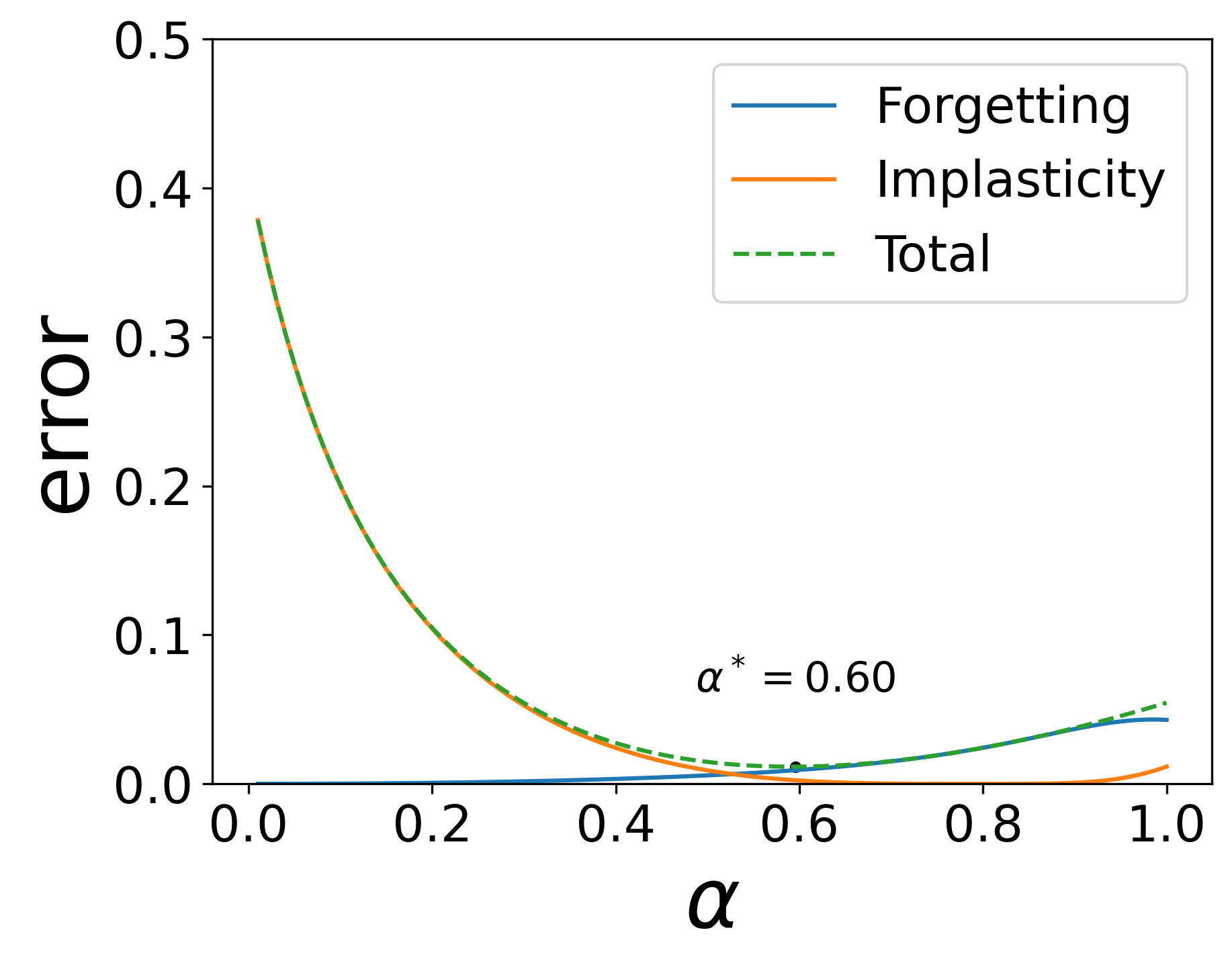
(a) $\eta=0.9$

(b) $\eta=0.95$

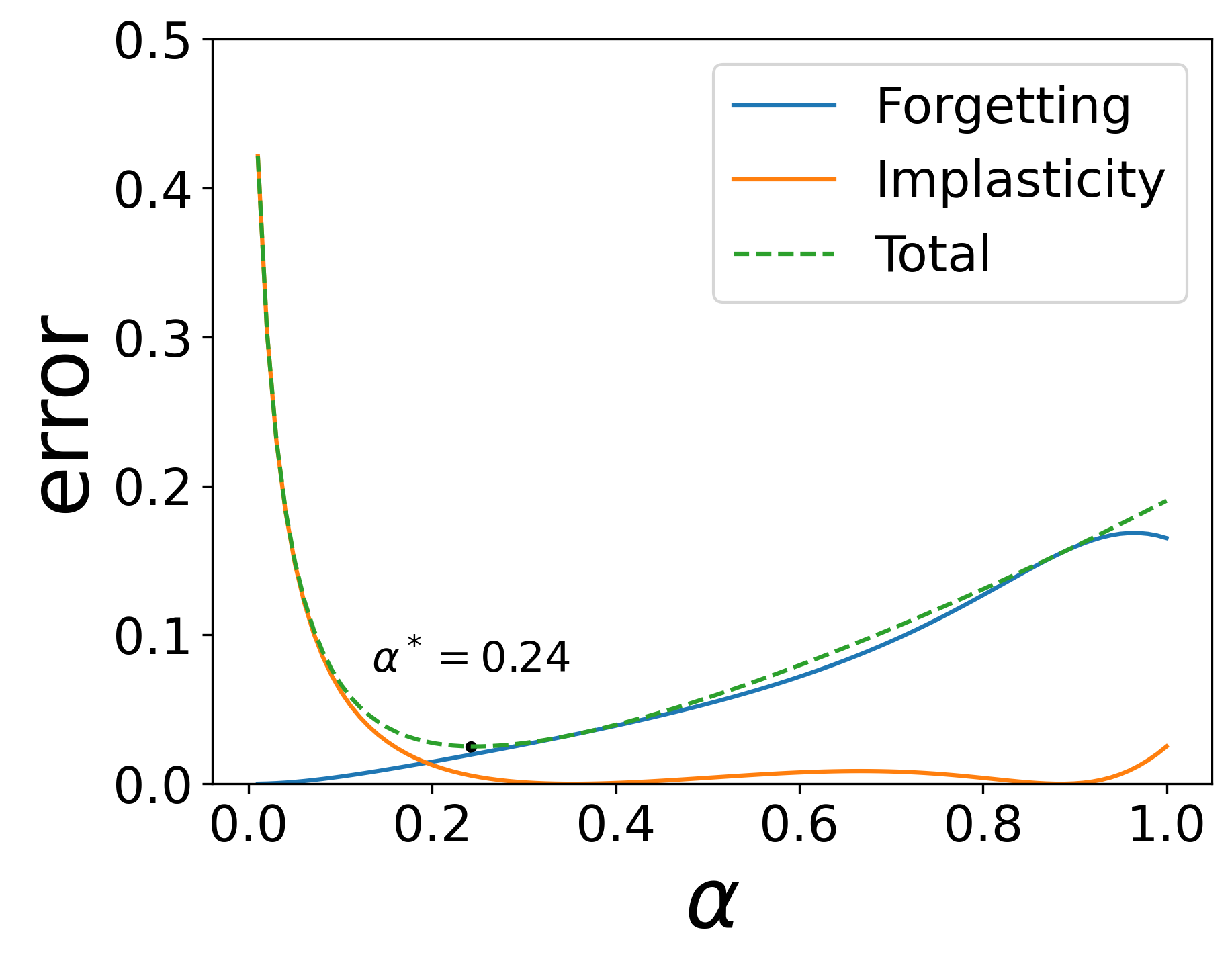
(c) $\eta=0.99$

Figure 5: Average forgetting and implasticity errors versus the stepsize $\alpha$ for environments with observation noise standard deviation $\sigma=0.5$, agent capacity $\mathbb{I}(U_{t};H_{t})=2$, and autoregressive model coefficients $\eta=0.9,0.95,0.99$. As $\alpha$ increases, the forgetting error increases and the implasticity error decreases, then the former decreases and the latter increases, albeit to much lesser extents. As $\eta$ increases, the optimal stepsize $\alpha^{*}$ decreases.

As $\alpha$ increases, the forgetting increases and the implasticity decreases. Then, as $\alpha$ approaches one, the former decreases and the latter increases, albeit to much lesser extents. It is natural for a small stepsize to reduce forgetting and implasticity since increasing the stepsize increases the weight placed on recent versus previously observed data. For the same reason, as the figure indicates, the optimal stepsize $\alpha^{*}$ decreases as $\eta$ increases. This is because a larger coefficient $\eta$ increases the mixing time of the process, and this warrants placing more weight on less recent observations to increase the duration over which they influence predictions.

Figure 6 plots the optimal stepsize as a function of $\eta$ (Figure 6(a)), the information capacity (Figure 6(b)), and the quantization noise intensity $\delta$ (Figure 6(c)). Note that we use $\alpha^{*}$ to represent the optimal stepsize for fixed $C$ and $\tilde{\alpha}$ for fixed $\delta$. As suggested by Figure 5, as $\eta$ increases, the optimal stepsize decreases. This makes sense since the mixing time of the AR(1) process scales with $1/(1-\eta)$, while the duration over which LMS averages observations scales with $1/\alpha$. As the mixing time grows, the optimal stepsize $\alpha^{*}$ decreases to induce averaging over longer durations. Interestingly, as demonstrated by the second plot, the optimal stepsize does not vary with the information capacity $C$. This observation is generalized and formalized by Theorem 15 in the appendix. It is interesting to note, however, that this does not imply invariance of the optimal stepsize to the quantization noise intensity $\delta$. In particular, when information content is unconstrained, the optimal stepsize varies with $\delta$, as demonstrated in Figure 6(c).

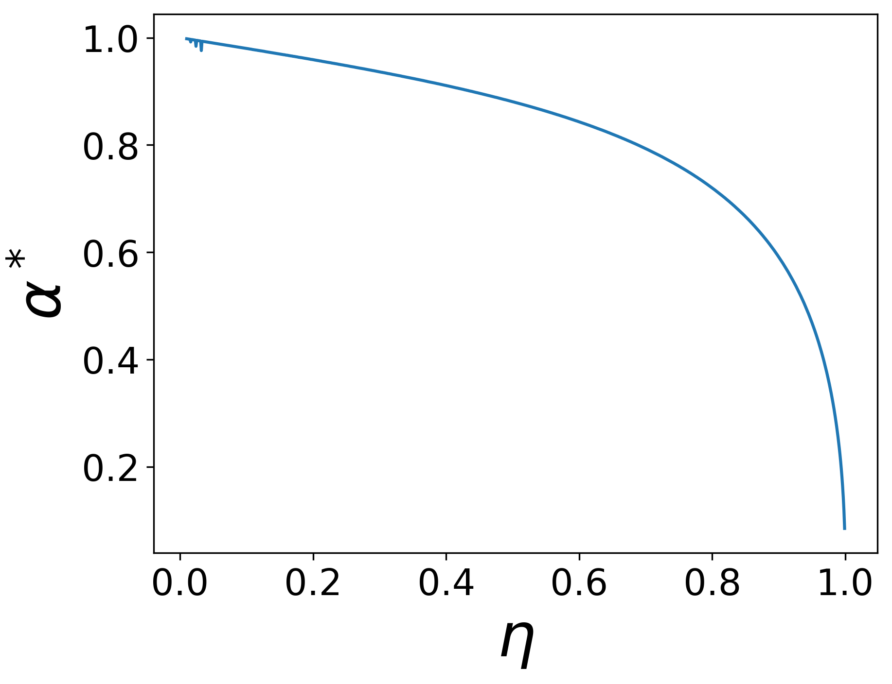
(a) $\alpha^{*}$ decreases $\eta$ increases.

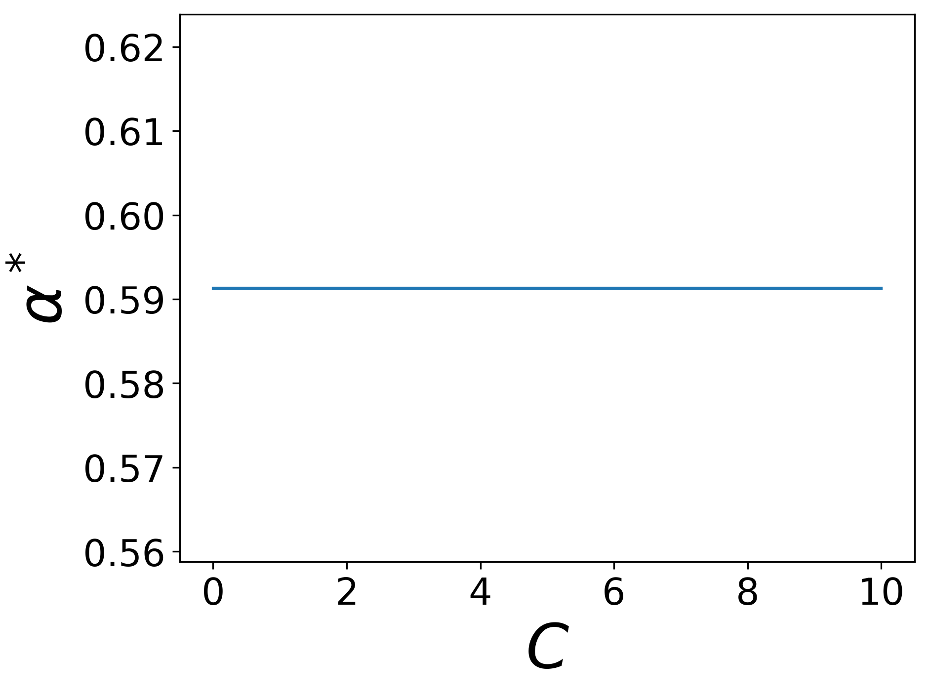
(b) $\alpha^{*}$ does not depend on $C$.

(c) $\tilde{\alpha}$ increases as $\delta$ increases.

Figure 6: As $\eta$ increases, so does the mixing time $1/(1-\eta)$. The optimal stepsize $\alpha^{*}$ decreases in response to induce averaging over a longer duration. The information capacity $C$ does not impact the optimal stepsize $\alpha^{*}$. However, the optimal stepsize $\tilde{\alpha}$ increases with the quantization noise standard deviation $\delta$. These plots are generated with observation noise $\sigma=0.5$. The center and right plots are generated with $\eta=0.9$. For the center plot, $\delta$ is chosen to meet the capacity constraint.

5.2.4 Stepsize Adaptation

Given a capacity constraint, calculating $\alpha^{*}$ requires knowledge of $\eta$. A stepsize adaptation scheme can alleviate this need, instead incrementally adjusting the stepsize to produce a sequence, aiming to converge on $\alpha^{*}$. As an example, we consider a variation of IDBD [Sutton, 1992]. In particular, suppose we update the agent state according to

$$U_{t+1}=U_{t}+\alpha_{t+1}(Y_{t+1}-U_{t})+Q_{t+1},$$

where $\alpha_{t+1}=e^{\beta_{t+1}}$ and $(\beta_{t}:t\in\mathbb{Z}_{++})$ is a scalar sequences generated according to

$$\beta_{t+1}=\beta_{t}+\zeta(Y_{t+1}-U_{t})h_{t}-\frac{1}{2}\zeta\alpha_{t}\frac{d}{d\alpha}\delta_{*}^{2}(\alpha_{t}),$$

$$h_{t+1}=\alpha_{t+1}(Y_{t+1}-U_{t})+(1-\alpha_{t+1})_{+}h_{t}.$$

The standard version of IDBD [Sutton, 1992] does not include the term that depends on $\delta_{*}$. This term serves to adjust the quantization noise variance in response to changes in the stepsize $\alpha_{t}$. For any particular stepsize $\alpha$, $\delta_{*}(\alpha)$ is the intensity at which the information capacity constraint $\mathbb{I}(U_{t};H_{t})\leq C$ becomes binding. Hence, ours is a capacity-constrained version of IDBD. The functional form of our extra term is derived in Appendix B.4.

Figure 7(a) demonstrates that capacity-constrained IDBD converges on the optimal stepsize for any given information capacity constraint. This limit of convergence identifies not only a stepsize $\alpha^{*}$ but also a quantization noise intensity $\delta_{*}(\alpha^{*})$. The standard version of IDBD, even if executed with quantization noise intensity fixed at $\delta=\delta_{*}(\alpha^{*})$, converges on a different stepsize, which is optimal for that intensity but not optimal subject to the capacity constraint. Consequently, as Figure 7(b) indicates, the error attained by capacity-constrained IDBD approaches the optimal error under the agent capacity, but does not with the standard version of IDBD.

(a) stepsize convergence.

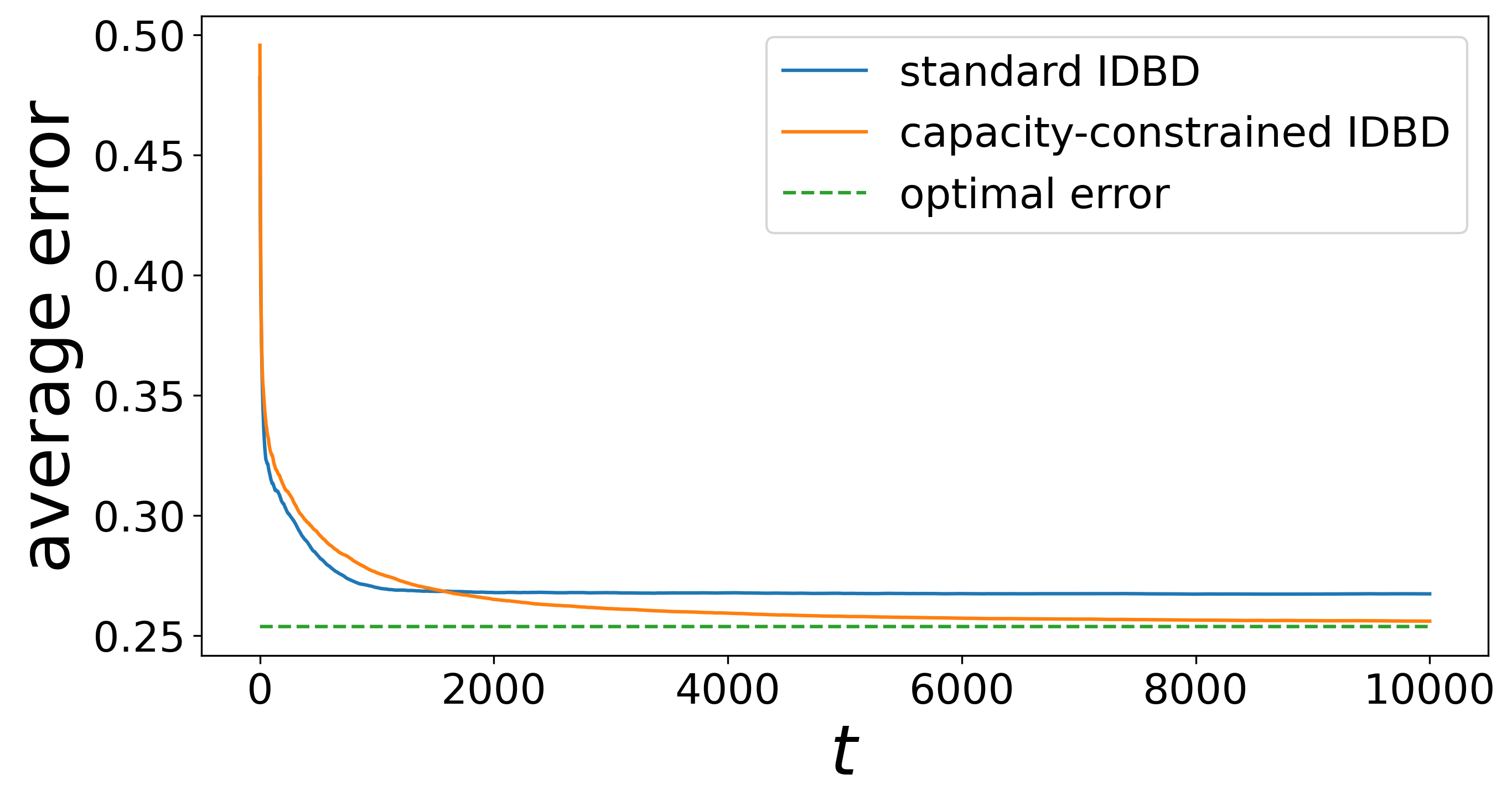
(b) error convergence.

Figure 7: Capacity-constrained IDBD converges on the optimal stepsize for the given capacity constraint. Even if the quantization noise intensity $\delta$ is fixed at the limiting value associated with this convergence, the standard version of IDBD converges on a different stepsize, which is optimal for that intensity. As such, while the error attained by capacity-constrained IDBD approaches the optimal error under the agent capacity, it does not with the standard version of IDBD. The plots are generated with $\zeta=0.01$, $\eta=0.95$, $\sigma=0.5$, $C=0.5$, and corresponding $\delta$ given by Theorem 12.

Updating $\beta_{t}$ relies on knowledge of the function $\delta_{*}$, which depends on $\eta$. This runs counter to the purpose of stepsize adaptation schemes, which ought to arrive at $\alpha^{*}$ without knowledge of $\eta$. However, the Gaussian noise $Q_{t+1}$ represents a simplified abstraction of quantization effects that would manifest if an agent were to encode information in finite memory. With a real encoding algorithm, the capacity constraint is physical and inevitable. As such, the agent need not itself derive the quantization noise intensity and thus may not require knowledge of $\eta$. How to devise effective stepsize adaptation schemes for practical capacity-constrained agents presents an interesting problem for future research.

A flaw in the narrative of this section is that it does not account for information capacity required to maintain $\alpha_{t}$, $\beta_{t}$, and $h_{t}$, which should be incorporated into the agent state $U_{t}$ if the agent implements capacity-constrained IDBD. In that event, the information capacity $C$ must support a joint quantized estimate of $\mu_{t}$ and these additional parameters. How information capacity should be managed in such situations remains an interesting subject for research.

Summary

• In continual supervised learning, the informational error $\mathbb{E}[{\mathbf{d}}_{\rm KL}(P^{*}_{t}\|\tilde{P}_{t})]$ can be decomposed into forgetting and implasticity:

  $$\underbrace{\mathbb{E}[{\mathbf{d}}_{\rm KL}(P^{*}_{t}\|\tilde{P}_{t})]}_{\mathrm{error}}=\sum_{k=0}^{t}\left(\underbrace{\mathbb{I}(Y_{t+1};U_{t-k-1}|U_{t-k},H_{t-k:t})}_{\mathrm{forgetting\ at\ lag\ }k}+\underbrace{\mathbb{I}(Y_{t+1};O_{t-k}|U_{t-k},H_{t-k+1:t})}_{\mathrm{implasticity\ at\ lag\ }k}\right).$$

  • The implasticity at lag $k$ measures the amount of information presented by $O_{t-k}$ that is useful for predicting $Y_{t+1}$ that the agent fails to ingest and is absent from the intermediate data $H_{t-k+1:t}$.

  • The forgetting at lag $k$ measures the amount of information useful for predicting $Y_{t+1}$ that the agent ejects when updating its agent state from $U_{t-k-1}$ to $U_{t-k}$ and is absent from the observations to be made before time step $t$, $H_{t-k:t}$.

• If each input $X_{t}$ is independent of history, i.e., $X_{t+1}\perp H_{t}$, and the sequence of agent states and observations forms a stationary stochastic process, the stability-plasticity decomposition implies that

  $$\lim_{t\to\infty}\underbrace{\mathbb{E}[{\mathbf{d}}_{\rm KL}(P^{*}_{t}\|\tilde{P}_{t})]}_{\mathrm{error}}=\lim_{t\to\infty}\left(\underbrace{\mathbb{I}(H_{t+1:\infty};U_{t-1}|U_{t},O_{t})}_{\mathrm{forgetting}}+\underbrace{\mathbb{I}(H_{t+1:\infty};O_{t}|U_{t})}_{\mathrm{implasticity}}\right).$$

  • The first term equates error due to forgetting with the information available in the previous agent state $U_{t-1}$, but unavailable in either in the subsequent agent state $U_{t}$ or the subsequent observation $O_{t}$.

  • The second term characterizes error due to implasticity as the information about the future $H_{t+1:\infty}$ available in the current observation $O_{t}$ but not ingested into the current agent state $U_{t}$.

6 Case Studies

Continual learning has broad scope, with potential applications ranging from recommendation and dialogue systems to robotics and autonomous vehicles. In Section 2.4, we framed continual learning as computationally constrained RL with an objective of maximizing average reward subject to constraints (Equation 3). This objective is designed to encompass real-world requirements of continual learning systems across applications. In this section, we study the implications of our objective on the design of performant continual learning agents.

To study these implications, we perform three case studies. Each case study highlights a different facet of continual learning: continual supervised learning, continual exploration, and continual learning with delayed consequences. In our first case study, we consider the special case of continual learning where the agent’s actions do not influence future observations. In particular, we study continual supervised learning, where an agent observes a nonstationary sequence of data pairs from its environment. The goal is to accurately predict labels $Y_{t+1}$ from inputs $X_{t}$. In other environments, such as bandits, the agent’s actions influence the agent’s immediate observations and therefore what information the agent is exposed to. Therefore, when selecting its next action, an agent should not only take into account the immediate reward (like in supervised learning), but also what information it can gain in order to perform well in the long term. Selecting actions for the purpose of acquiring new information is known as exploration. In our second case study, which is on continual exploration, we study the implications of nonstationarity for exploration. Our third case study focuses on the broader class of environments in which actions induce not only immediate consequences but also delayed consequences. We call this continual learning with delayed consequences. In each case study, we perform simple illustrative experiments to develop intuitions for what behaviors a performant continual learning agent might need.

6.1 Continual Supervised Learning

In this section, we consider the continual supervised learning setting, which has been the focus of most prior work in continual learning. In continual supervised learning, an agent receives a nonstationary sequence of data pairs from its environment, and the agent’s actions do not influence the data sequence. The agent’s goal is to make accurate predictions on the observations it receives. As an example, consider a fraud detection system for credit card transactions. The goal of such a system is to classify transactions as fraudulent or not fraudulent. The techniques people use to commit fraud and evade detection may evolve over time, and the system must adapt to these changing fraud patterns.

Research in continual supervised learning over the years has proposed synthetic problems for comparing and evaluating different agent designs. For instance, an agent may be learning to classify digits and over time the digits may rotate [Buzzega et al., 2020]. On such problems, a common evaluation protocol is to periodically measure the agent’s performance on all types of data seen so far. In the digit classification example, the agent’s prediction accuracy is evaluated on digits with previously encountered rotation angles. Though not stated explicitly, this means that the agent’s objective is to learn about and remember everything in the past.

However, as we have mentioned before, this objective — to remember everything — is neither feasible nor necessary. In the real world, the goal is to do well on future tasks, not on those in the past. In the fraud detection example, some fraud techniques may become outdated or impossible to use due to new security measures, and the system may not need to remember how to handle those types of cases. Generally, in a dynamic environment, some knowledge becomes obsolete and not necessary to remember. Further, intelligent systems will be computationally constrained in practice and cannot remember everything. Our average-reward objective under computational constraints tries to capture these real-world requirements. Importantly, this objective has multiple implications for continual supervised learning, especially with regard to forgetting and plasticity.

In this section, we perform a set of simple experiments on a synthetic problem to highlight some of the implications of our average-reward objective in the continual supervised learning setting. We specifically study the impact of forgetting when information recurs and when the agent is computationally constrained. Through our experiments, we make the following points: (1) a performant agent can forget non-recurring information, (2) a performant agent can forget recurring information if it relearns that information quickly, and (3) under tight computational constraints, forgetting may be helpful.

6.1.1 Environment

We perform our experimental evaluation on a modified version of Permuted MNIST, a common benchmark from the continual learning literature [Goodfellow et al., 2013]. Permuted MNIST is characterized by a sequence of training datasets. Each dataset is constructed in two steps: (1) we randomly sample a permutation over all pixels, and (2) we apply this permutation to every image from the standard MNIST training dataset. Each such permuted training set is referred to as a task.

In our experiments, we aim to study the role of both non-recurring and recurring information on agents’ performance, since it is only to the extent that information recurs that it is worthwhile to remember. Equivalently, there may be forward transfer, meaning information from previous tasks can be leveraged to do well on future tasks. On the Permuted MNIST benchmark, it is conceivable that there is some forward transfer (e.g. if the network learns permutation invariant features to classify digits). To design controlled experiments in which it is clear which information recurs and which information does not, we create a modified version with minimal forward transfer. Specifically, we additionally permute the labels randomly in each task. For instance, all the images with label $3$ may get assigned a different label, such as $5$. On this version of Permuted MNIST, most information by default is non-recurring.

In this setup, a continual learning data sequence consists of a sequence of tasks. In turn, each task consists of $k$ batches of images with one batch arriving at every time step. Each incoming batch from the data sequence contains $b_{\text{env}}$ images, where the subscript env is shorthand for “environment.” In our experiments, $b_{\text{env}}=16$. We call the number of time steps a task occurs before switching to the next task the task duration.

While the Permuted MNIST benchmark is typically characterized by a sequence of permutations where each permutation occurs once, we consider a particular type of environment dynamics that exhibits periodic recurrence. Specifically, on our version of Permuted MNIST, the first permutation recurs periodically: every alternate task is the first permutation, while all other tasks are determined by new permutations which do not recur. As an example, given $100$ permutations P1, P2, …, P100 the sequence of tasks may look like P1, P2, P1, P3, P1, P4, P1, P5, …. Note that since we have minimized forward transfer between permutations by permuting labels in addition to input pixels, we can study the effect of information recurrence specifically induced by the first permutation recurring.

6.1.2 Agents

A common agent design that improves an agent’s ability to retain past information in continual supervised learning is to equip the agent with a replay buffer [Aljundi et al., 2019, Buzzega et al., 2020, Chaudhry et al., 2019, Chrysakis and Moens, 2020, Yoon et al., 2021]. The agent may use this buffer to store past data pairs and continue extracting information from them. In line with this approach, we consider three simple agents which store data in a replay buffer and are trained using SGD. We constrain all agents to perform a single SGD step per time step. The agents perform each SGD step on a batch containing both incoming data ($b_{\text{env}}$ data pairs) and data sampled uniformly from the replay buffer ($b_{\text{replay}}$ data pairs). All agents use so-called reservoir insertion to add data to the buffer, which ensures that the full buffer is a random sample from the full history [Vitter, 1985]. Specifically, given the buffer size $B$ and length $T$ of the entire history $H_{T}$, reservoir insertion guarantees each data pair has the same probability $\frac{B}{T}$ of being stored in the buffer, without knowing the length of the entire data stream in advance. This strategy is common practice in the design of continual learning agents with a limited capacity replay buffer [Buzzega et al., 2020, Koh et al., 2023].

The three agents are Large Memory , which has a buffer size of $1$ million data pairs, Small Memory, which can store only $1,000$ data pairs, and Reset, which has the same replay buffer size as Large Memory but periodically resets all agent components (the neural network parameters are re-initialized and the buffer is emptied). In experiments where we study the effect of resetting, we refer to the Large Memory agent as No Reset. For all agents, we use a $2$ hidden layer neural network with hidden layer width $1000$, and we set $b_{\text{replay}}=16$.

6.1.3 Evaluation Protocol

Most works in continual supervised learning evaluate agents on their performance on previous tasks. In contrast, we evaluate agents on their ability to maximize average reward, which is in line with previous work that considers the online continual learning setting [Cai et al., 2021, Ghunaim et al., 2023, Prabhu et al., 2023a]. Because the primary goal in supervised learning is often to achieve good accuracy, we let the reward function be online accuracy. Our objective is thus to maximize average online accuracy under computational constraints. Using the notation presented in Section 2, this objective can be written as follows:

$$\begin{array}[]{ll}\max_{\pi}&\liminf_{T\rightarrow\infty}\mathbb{E}_{\pi}\left[\frac{1}{T}\sum_{t=0}^{T-1}\mathbbm{1}(Y_{t+1}=\hat{Y}_{t+1})\right]\\ \text{s.t.}&\text{computational constraint}\end{array}$$

where at each time step $t$, $Y_{t+1}$ is the true label of observation $X_{t}$, $\hat{Y}_{t+1}\in\operatorname*{arg\,max}_{y}P_{t}(y\in\cdot)$ is the agent’s predicted label, and $\mathbbm{1}$ is the indicator function.

Our average reward objective is the limit of an expectation that integrates over a growing sequence, which in most cases is infeasible to compute. Instead, we will evaluate an approximation by (1) limiting the duration of interaction and (2) approximating the expectation by averaging over a finite number of sequences. We propose a variation of the train/test protocol used in supervised learning. First, we split the data into two parts: a single development sequence and a set of evaluation sequences. We use the development sequence to tune an agent by varying hyperparameters. After selecting the best hyperparameters based on the development sequence, we reset the agent (re-initialize the neural network and replay buffer) and train the agent on the evaluation sequences. Finally, the agent’s performance is averaged across all evaluation sequences.

In accordance with this evaluation protocol, on our modified Permuted MNIST environment, we split all data into two subsets, one used to generate the development sequence and the second used to generate evaluation sequences. Each subset contains $100$ permutations, and the two subsets do not share any permutations. Consequently, there is no overlap in permutations between the development sequence and the evaluation sequences. Each permutation has $400$ unique data pairs, for a total of $40,000$ unique data pairs per subset of data. On each subset of data, we train agents over $3$ random seeds, where the seed determines both the initialization of the agent and the generated sequence of data pairs the agent receives from that subset. We perform hyperparameter tuning on the development sequence and report evaluation performance averaged over all $3$ seeds (and therefore $3$ evaluation sequences). For additional details on the environments and evaluation protocol, see Appendix C.1.

6.1.4 Results

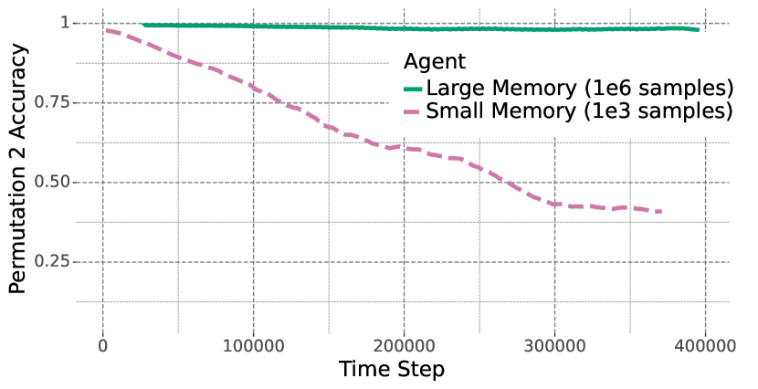
(a) Performance on Permutation $2$

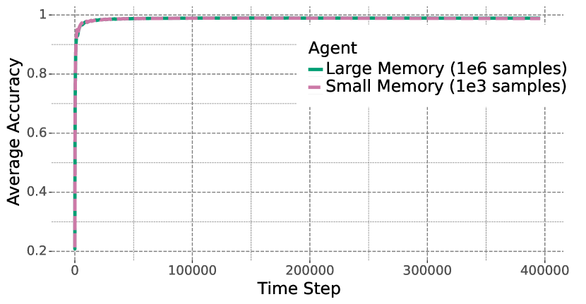
(b) Average Accuracy

Figure 8: (a) Performance on Permutation $2$, which is a non-recurring task. For this plot, the agent’s accuracy is computed and averaged across all data points of Permutation $2$. Large Memory remembers previous information, whereas Small Memory forgets. (b) Average accuracy. Despite this difference in forgetting, the two agents perform similarly under our objective. The key reason for this result is that in this environment there is little benefit to remembering non-recurring tasks in order to perform well.

A performant agent can forget non-recurring information. We consider a case in which each task has a duration of $2,000$ time steps. This corresponds to the agent seeing each data pair from a task approximately $100$ times, which allows the agent to achieve $100\%$ accuracy on each task. We consider this setting so that we can study the effects of forgetting after an agent completely learns each task.

On this variant of Permuted MNIST, we evaluate the Large Memory and Small Memory agents (Figure 8). While Small Memory forgets previous non-recurring information quickly relative to Large Memory, both agents perform similarly under our objective. This result highlights that a performant agent can forget information that is non-recurring. In particular, if a task does not occur more than once and the information required to successfully complete the task is not useful for any future tasks, there is no benefit to remembering this information. Since our version of Permuted MNIST permutes both input pixels and labels, there is little transfer of information between classifying digits with one permutation versus another. Therefore, it is reasonable to forget how to accurately predict labels for non-recurring permutations.

While this experiment is simple, the result helps clarify the role of forgetting in continual supervised learning. In the continual learning literature, catastrophic forgetting is highlighted as a critical issue, and performance on previous tasks is the primary metric used in prior work to evaluate methods [Wang et al., 2023]. We argue that when discussing forgetting, it is important to recognize that the usefulness of a (perhaps large) subset of information in real-world applications is transient. Forgetting this information is not catastrophic.

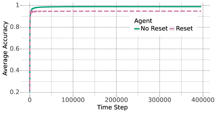
(a) Short Task Duration ($2$k time steps)

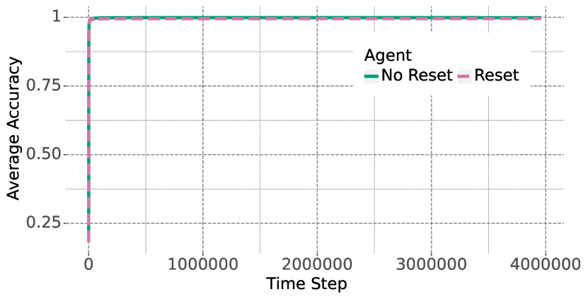
(b) Long Task Duration ($20$k time steps)

Figure 9: (a) Average accuracy when each task duration is short. When each task duration is short there is relatively little time to exploit information after it has been learned, and the performance of Reset suffers relative to No Reset, which doesn’t forget. (b) Average accuracy when each task duration is long. When each task duration is long, the time to learn is short relative to the task duration. Therefore, Reset and No Reset perform similarly.

A performant agent can forget recurring information if it relearns that information quickly. We evaluate the No Reset and Reset agents with two different permutation durations: $2,000$ time steps and $20,000$ time steps (Figure 9). The Reset agent forgets all information, both recurring and non-recurring, after each permutation. However, when permutation durations are long, its performance under our objective only suffers slightly compared to the performance of No Reset, which remembers recurring information. This is because the Reset agent is able to relearn the recurring task quickly relative to the duration of the task. This result is in line with Ashley et al. [2021] which highlights that we need to consider different measures when considering forgetting, including retention and the ability to relearn quickly. Further, the average reward objective resolves the extent to which each of these agent characteristics matters. For instance, the duration of information’s utility is an important factor.

Under tight computational constraints, forgetting may be helpful. In machine learning, an agent is often parameterized by a neural network, and all parameters of the neural network are updated when taking gradient steps on data pairs. Given this protocol, a computational constraint per time step, which limits the number of FLOPS when updating the neural network, effectively limits the physical capacity of the neural network the agent can use. Tight computational constraints therefore induce capacity constraints.

To study this setting, we consider reductions in the size of the neural network so that the SGD step of each iteration can be executed within tighter computation budgets. Concretely, in addition to a hidden size of $1000$, we use smaller hidden sizes of $100$, $25$, and $10$. With these smaller network architectures, we evaluate the No Reset and Reset agents where each task has a duration of $20,000$ time steps (Figure 10). We find that as the capacity decreases, No Reset begins to outperform Reset. We see that when the hidden size is $10$, the performance of No Reset decreases over time as there is insufficient capacity to both remember everything and continue updating on new data. In particular, No Reset suffers from loss of plasticity, a characteristic of neural networks that has been studied in recent work [Dohare et al., 2021, Lyle et al., 2023, Nikishin et al., 2023]. In contrast, because Reset re-initializes the neural network and replay buffer periodically, it retains high plasticity and therefore outperforms No Reset.

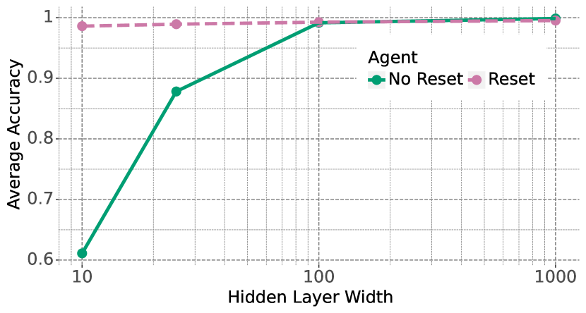
(a) Hidden Layer Width vs Average Accuracy

(b) Average Accuracy when Hidden Layer Width = 10

Figure 10: (a) Average accuracy at the end of evaluation when the neural network has different hidden layer widths. As the agent becomes increasingly capacity constrained (smaller hidden layer width), forgetting becomes more beneficial. (b) Average accuracy over time when the hidden layer width is $10$. When the agent is severely capacity constrained, resetting prevents loss of plasticity.

6.2 Continual Exploration

In supervised learning environments, such as those studied in Section 6.1, an agent’s actions do not influence future observations. As a result, the information available to an agent does not depend on its agent policy. However, in more general classes of environments, actions do influence observations. In such environments, active exploration may be required to attain strong performance, as different actions can expose the agent to different information.

As an example, when a recommendation system recommends items to its users, the user behavior the system observes will vary depending on the recommendations it makes. To improve the quality of recommendations in the long term, a recommendation system may benefit from suggesting a diverse range of items to new users, enabling it to learn more about user preferences.

While seeking out new information can be helpful in the long run, exploration often induces a cost in the short term. Specifically, an agent may sacrifice immediate reward. For instance, a recommendation system may have to recommend multiple different items to a user until it identifies the full range of item types that the user likes. While this is great for the user (and the recommendation system) in the long term, in the short term, the user ends up recommended a host of items they may not like. This trade-off between seeking out information and optimizing immediate reward is commonly known as the exploration-exploitation trade-off. Agents must strike a balance between exploring to seek out information and exploiting existing information to optimize immediate performance.

This problem of balancing exploration and exploitation has primarily been studied in the context of vanishing-regret learning. In this section, we will instead study exploration in the context of continual learning. Specifically, we investigate the implications that nonstationarity has for intelligent exploration. We will argue through didactic examples and simulations that in order to perform well in a nonstationary environment, an agent should (1) continuously engage in exploration, (2) prioritize seeking out information that remains useful over an extended period, and (3) learn about the environment dynamics to guide exploration.

6.2.1 Exploration in Stationary Environments

Before considering the implications that nonstationarity has for exploration, let us first consider exploration in a stationary setting. In a typical stationary environment, the degree to which a performant agent explores typically decreases over time. In other words, an agent acquires progressively less information as time goes on. For instance, in some stationary environments, the total amount an agent needs to learn to attain optimal or near-optimal average reward is bounded. In such an environment, the amount of information acquired per time step vanishes as time progresses.

To illustrate the trade-off between exploration and exploitation, as well as the typical decrease in exploration over time in a stationary environment, let us examine a special case of the coin tossing example previously discussed in Example 1. Suppose that the bias $p_{1}=0.8$ of coin $1$ is known, and the prior distribution over the bias of coin $2$ is uniform dyadic over the set $\{0,1\}$. Consequently, at each time $t$ before coin $2$ is tossed, the bias $p_{2}$ is distributed according to a uniform distribution over $\{0,1\}$; once coin $2$ is tossed, the belief distribution of $p_{2}$ is updated to concentrate on the outcome of the toss. These environment dynamics are characterized by a function $\rho$, defined as follows. For $a=1$, $\rho(1|h,a)=0.8$. For $a=2$, $\rho(1|h,a)=p_{2}$ if coin $2$ was previously tossed according to $h$, and otherwise, $\rho(1|h,a)=0.5$.

In this example, an agent can benefit from learning about the bias $p_{2}$ associated with coin $2$. Once the coin is tossed and its bias is revealed, the agent can consistently select the better coin. However, the act of exploring and learning about $p_{2}$ comes at a cost of sacrificing immediate reward; the expected reward of tossing coin $2$ is only $0.5$, significantly lower than the expected reward of $0.8$ associated with coin $1$. It is worth mentioning that this example also illustrates the typical decrease in exploration over time in a stationary environment. Indeed, this example presents an extreme case where an agent is “done” with exploring and learning about $p_{2}$ after the first toss of coin $2$.

6.2.2 Exploration in Nonstationary Environments

In nonstationary environments, the nature of exploration differs from that of in stationary environments. Here, we outline three key implications of nonstationarity on exploration:

1. Never stop exploring. In a typical nonstationary environment, new information continually arrives. Crucially, there is usually a non-diminishing supply of new and valuable information. As a result, it is common for an optimal agent to engage in continuous exploration to learn about such information. This is in direct contrast to the stationary setting, where agents tend to reduce their exploration over time.

   This idea has been explicitly or implicitly discussed in prior nonstationary bandit learning or nonstationary reinforcement learning literature. For example, many nonstationary learning algorithms are designed to learn a different latent variable at each time, e.g. a different mean reward or a different MDP. For this purpose, many nonstationary bandit learning algorithms estimate a mean reward and then adopt a stationary bandit learning algorithm as a subroutine [Besbes et al., 2019, Besson and Kaufmann, 2019, Cheung et al., 2019, Garivier and Moulines, 2008, Ghatak, 2021, Gupta et al., 2011, Hartland et al., 2006, Kocsis and Szepesvári, 2006, Mellor and Shapiro, 2013, Raj and Kalyani, 2017, Trovo et al., 2020, Viappiani, 2013].

2. Seek out durable information. While new information continually arrives in a typical nonstationary environment, it is important to recognize that some information may be transient and lose its relevance over time. In order to succeed in a nonstationary environment, an agent must prioritize seeking out information that remains valuable and relevant for a longer duration. We refer to this characteristic as durability, which represents the degree to which an agent’s acquired information remains useful over time. More precisely, an agent should deprioritize acquiring information that is less durable.

   The concept of information durability was introduced by [Liu et al., 2023b]. This work also emphasizes the importance of an agent intelligently considering the durability of information when selecting actions, through coin tossing games, theoretical results, and simulation experiments.

3. Learn about environment dynamics to guide exploration. In order to seek out information that is more durable, an agent needs to determine the durability of information. To achieve this, an agent can benefit from dedicating a portion of its computational budget to learning about aspects of the environment dynamics that determine the durability of information.

6.2.3 Coin Swapping Games

We examine three coin swapping examples to illustrate these three implications that nonstationarity has on exploration. These examples are variants of the coin tossing example described in Section 6.2.1. Recall that the bias $p_{1}=0.8$ of coin $1$ is known, and the prior distribution over the bias of coin $2$ is uniform dyadic over the set $\{0,1\}$. The key difference is that now in the coin swapping examples, the second coin is replaced at each time step with probability $q_{2}$. The coin replacement probability $q_{2}$ varies across the three examples. Note that these games also serve as specific instances of Example 2, where the prior distributions over the bias of each coin are provided in Section 6.2.1.

Small replacement probability. Let us first consider a game where the coin replacement probability $q_{2}$ for coin $2$ is known to the agent and is small, for instance $q_{2}=0.001$. In this game, before coin $2$ is tossed for the first time, the expected reward from selecting coin $2$ is $0.5$. If the agent has selected coin $2$, and the latest outcome is tails, then the expected reward from selecting coin 2 is $0.0005$. In both of these cases, the expected reward from selecting coin 2 is much smaller than the expected reward of $0.8$ associated with coin $1$. In addition, the bias of coin $1$ is known, so selecting coin $2$ in this context exemplifies exploration.

Despite that coin $2$ is associated with a lower expected reward, an optimal agent should eventually select coin $2$, because it is very likely that the coin has eventually been replaced, possibly with a new coin of bias $1$. If the new coin does indeed have a bias of $1$, selecting coin $2$ allows the agent to learn about this bias and then continue selecting the same coin, resulting in a reward of $1$ for a long time—an average of $1000$ consecutive time steps. Since selecting coin $2$ exemplifies exploration, this game serves as an illustration that an optimal agent may need to continuously explore, unlike in stationary environments.

Large replacement probability. Next, suppose that the coin replacement probability $q_{2}$ for coin $2$ is instead large, say, $q_{2}=0.999$. Because coin $2$ is likely to be replaced at each time, the information associated with it quickly becomes obsolete. In other words, the information is not very durable. Therefore, unlike in the previous game, an agent does not benefit from learning about the bias of coin $2$ anymore in this game. Indeed, an optimal agent will only ever select coin $1$ throughout the entire game. This variation highlights the importance of only seeking out information to the extent that the information is durable.

Unknown Replacement Probability Now suppose that the coin replacement probability $q_{2}$ for coin $2$ is unknown. This presents a typical scenario where an agent does not know the environment dynamics a priori. Recalling the previous two variations of the coin-swapping game, we observe that the optimal behaviors differ significantly based on this coin replacement probability. This indicates that understanding and learning about the coin replacement probability is crucial for determining the durability of information and selecting actions accordingly. This variation of the game emphasizes the importance of learning about the dynamics of the environment in order to guide exploration. By acquiring knowledge about the coin replacement probability, an agent can make informed decisions on how to explore and seek out durable information in a nonstationary environment.

6.2.4 Experiments in AR(1) Bandits

While the coin tossing games serve as a model of environments with abrupt changes and bounded rewards, our insights on continual exploration extend beyond such settings. To demonstrate this, we conduct experiments in a class of Gaussian bandits that capture continuous or smooth changes in environments with unbounded rewards. These bandits are known as AR(1) Gaussian bandits, and Example 4 in Section 2.3 serves as one specific instance of an AR(1) Gaussian bandit. The AR(1) bandits or similarly constructed nonstationary Gaussian bandits have been studied by Gupta et al. [2011], Kuhn et al. [2015], Kuhn and Nazarathy [2015], Liu et al. [2023b], Slivkins and Upfal [2008].

Environment

We consider a two-armed Gaussian bandit described in Example 4. Recall that the environment is characterized by latent random variables $\theta_{0,a}$ independently and initially distributed $\mathcal{N}(\mu_{0,a},\Sigma^{2}_{0,a})$, and updated according to

$$\theta_{t+1,a}=\eta\theta_{t,a}+Z_{t+1,a},$$

with each $Z_{t+1,a}$ independently sampled from $\mathcal{N}(0,\zeta^{2})$. Each reward $R_{t+1}=O_{t+1}=\theta_{t,A_{t}}+W_{t+1,A_{t}}$, where each $W_{t+1,a}$ is sampled independently from $\mathcal{N}(0,\sigma^{2})$. The parameters of the environment include the prior mean $\mu_{0,a}\in\mathbb{R}$, the prior variance $\Sigma_{0,a}\in\mathbb{R}_{+}$, the AR(1) parameter $\eta\in\mathbb{R}$, the $Z_{t,a}$ variance $\zeta^{2}\in\mathbb{R}_{+}$, and the observation noise variance $\sigma^{2}\in\mathbb{R}_{+}$.

In our experiments, we let $\mu_{0,a}=0$, $\Sigma_{0,a}=1$, $\sigma=1$, and $\zeta$ be such that each sequence $(\theta_{t,a}:t\in\mathbb{N})$ is a stationary stochastic process. The AR(1) parameter $\eta$ is the remaining parameter that we vary across experiments. It determines the degree to which information about $\theta_{t,a}$ is durable; if $\eta=1$, then the information about $\theta_{t,a}$ remains useful forever, and if $\eta=0$, then the information immediately lose its relevance at the next time step.

Agents

We consider two agents: Thompson sampling [Thompson, 1933], which does not take into account the durability of information when selecting actions, and predictive sampling [Liu et al., 2023b], which does. Both agents have privileged access to the environment parameters.

Thompson sampling. First, we consider the Thompson sampling agent, which was introduced in Example 4. This agent is representative of those which do not account for the durability of information. Recall that the agent maintains a posterior distribution of $\theta_{t,a}$ for each action $a$, parameterized by $\mu_{t,a}$ and $\Sigma_{t,a}$. Thompson sampling updates these parameters according to the equations presented in Section 2.3.2, Example 4. We restate the equations below:

$$\mu_{t+1,a}=\left\{\begin{array}[]{ll}\eta\mu_{t,a}+\alpha_{t+1}(O_{t+1}-\eta\mu_{t,a})&\mathrm{if\ }a=A_{t}\\ \eta\mu_{t,a}&\mathrm{otherwise,}\end{array}\right.\qquad\Sigma_{t+1,a}=\left\{\begin{array}[]{ll}\frac{1}{\frac{1}{\eta^{2}\Sigma_{t,a}+\zeta^{2}}+\frac{1}{\sigma^{2}}}&\mathrm{if\ }a=A_{t}\\ \eta^{2}\Sigma_{t,a}+\zeta^{2}&\mathrm{otherwise,}\end{array}\right.$$

where $\alpha_{t+1}=\Sigma_{t+1,A_{t}}/\sigma^{2}$. The agent then estimates mean rewards and selects the action corresponding to the largest estimate by sampling each $\hat{\theta}_{t,a}$ independently from $\mathcal{N}(\mu_{t,a},\Sigma_{t,a})$, and selecting an action uniformly at random from the set $\arg\max_{a\in\mathcal{A}}\hat{\theta}_{t,a}$.

Predictive sampling. The other agent that we consider is a predictive sampling agent. Predictive sampling can be viewed as a modified version of Thompson sampling that de-prioritizes transient information. In an AR(1) bandit, specifically, similar to the Thompson sampling agent, this agent maintains the same set of hyperparameters, and also updates parameters $\mu_{t+1,a}$ and $\Sigma_{t+1,a}$ according the equations above. The parameters determine the posterior belief of $\theta_{t,a}$. Different from Thompson sampling, the agent then samples each $\hat{\theta}_{t,a}$ independently from a different distribution, i.e., $\mathcal{N}(\tilde{\mu}_{t,a},\tilde{\Sigma}_{t,a})$, and selects an action uniformly from the set $\arg\max_{a\in\mathcal{A}}\hat{\theta}_{t,a}$.

Specifically, predictive sampling updates the parameters $\tilde{\mu}_{t,a}$ and $\tilde{\Sigma}_{t,a}$ of its sampling distribution as follows:

$$\ \tilde{\mu}_{t,a}=\mu_{t,a}\text{ and }\tilde{\Sigma}_{t,a}=\frac{\eta_{a}^{2}\Sigma_{t,a}^{2}}{\eta_{a}^{2}\Sigma_{t,a}+x_{a}^{*}},$$

where $x_{a}^{*}=\frac{1}{2}\left(\zeta_{a}^{2}+\sigma^{2}-\eta_{a}^{2}\sigma^{2}+\sqrt{(\zeta_{a}^{2}+\sigma^{2}-\eta_{a}^{2}\sigma^{2})^{2}+4\eta_{a}^{2}\zeta_{a}^{2}\sigma^{2}}\right)$.

The update expression for $\tilde{\Sigma}_{t,a}$ is quite involved, so we provide some intuition for how predictive sampling behaves relative to Thompson sampling. We first consider the case where $\eta=1$. This corresponds to a stationary environment. In this setting, predictive sampling executes the same policy as Thompson sampling because $\tilde{\Sigma}_{t,a}=\Sigma_{t,a}$.

On the other extreme, if $\eta=0$, $\theta_{t,a}$ is completely determined by the process noise. This corresponds to an environment where information about $\theta_{t,a}$ is completely not durable. In this setting, predictive sampling’s sampling variance $\tilde{\Sigma}_{t,a}$ for each arm $a$ is $0$, and this agent therefore executes a greedy policy.

More generally, the predictive sampling agent’s sampling variance $\tilde{\Sigma}_{t,a}$ lies between $0$ and $\Sigma_{t,a}$, i.e., $0\leq\tilde{\Sigma}_{t,a}\leq\Sigma_{t,a}$. In addition, the ratio $\tilde{\Sigma}_{t,a}/\Sigma_{t,a}$ is monotonically increasing in $\eta$. Therefore, predictive sampling samples actions from distributions with smaller variances as compared to that of Thompson sampling. This corresponds to more exploitation versus exploration. In summary, in an AR(1) bandit, predictive sampling can be viewed as a variant of Thompson sampling that adjusts how it balances exploration and exploitation according to $\eta$, which determines the durability of information. The behavior of PS is motivated by the fact that when information about $\theta_{t,a}$ is less durable, meaning that $\theta_{t,a}$ is less informative in predicting $(\theta_{k,a}:k\geq t+1)$, an agent should deprioritize acquiring information about $\theta_{t,a}$.

Results

We conduct two experiments to investigate the impact of information durability on agent performance. In the first experiment, we compare the performance of predictive sampling and Thompson sampling over time. The results demonstrate that predictive sampling consistently outperforms Thompson sampling. Furthermore, we observe that predictive sampling tends to take greedy actions more frequently; here, greedy actions refer to actions with higher mean reward estimates. This finding supports our hypothesis that de-prioritizing transient information leads to improved performance.

In the second experiment, we examine the performance gap between the two agents in environments with varying levels of information durability. The results reveal that the performance gap between the two agents is more significant in environments where information is less durable. This suggests that the choice of exploration strategy becomes even more critical when information is less durable.

Recall that the environments we examine are parameterized by $\eta$, which determines the degree to which information about $\theta_{t,a}$ is durable. In such environments, the information durability associated with different actions are comparable, and deprioritizing transient information translates to deprioritizing exploration relative to exploitation as information durability decreases.

De-prioritizing transient information is beneficial. Figure 11(a) plots the action selection frequencies against time, and the band corresponds to 95% confidence band. This figure shows that predictive sampling consistently selects greedy actions more than Thompson sampling. Figure 11(b) plots the average reward collected by each agent against time ($t=1,...200$). This figure shows that predictive sampling consistently outperforms Thompson sampling across time. The two plots suggest that de-prioritizing transient information, which in this environment corresponds to exploiting more by taking more greedy actions, leads to better performance in nonstationary environments.

The benefit is larger in environments with less durable information. Figure 12(a) plots the action selection frequency of each agent over $200$ time steps against the AR(1) parameter. The figure shows that the gaps between the action selection frequences also increase as the AR(1) parameter decreases, i.e., as information becomes less durable. Figure 12(b) plots the average reward collected by each agent over $200$ time steps against the AR(1) parameter. The figure shows that the performance gap between the agents increase as the AR(1) parameter decreases, i.e., as information becomes less durable. The two plots suggest that the performance gain from deprioritizing less durable information is larger in environments where information is less durable.

These experiments provide valuable insights into the relationship between information durability and agent performance, further reinforcing the importance of intelligent exploration in nonstationary environments.

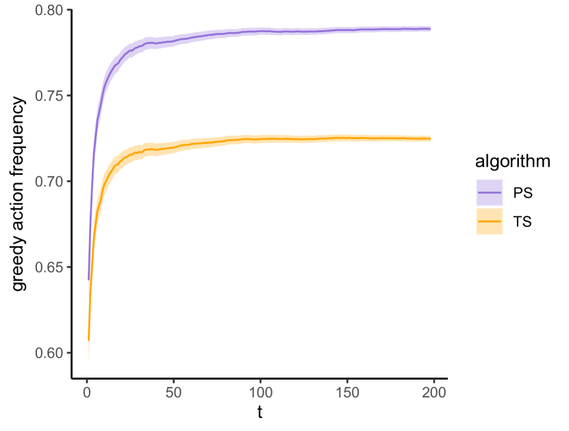
(a) Greedy Action Selection Frequencies

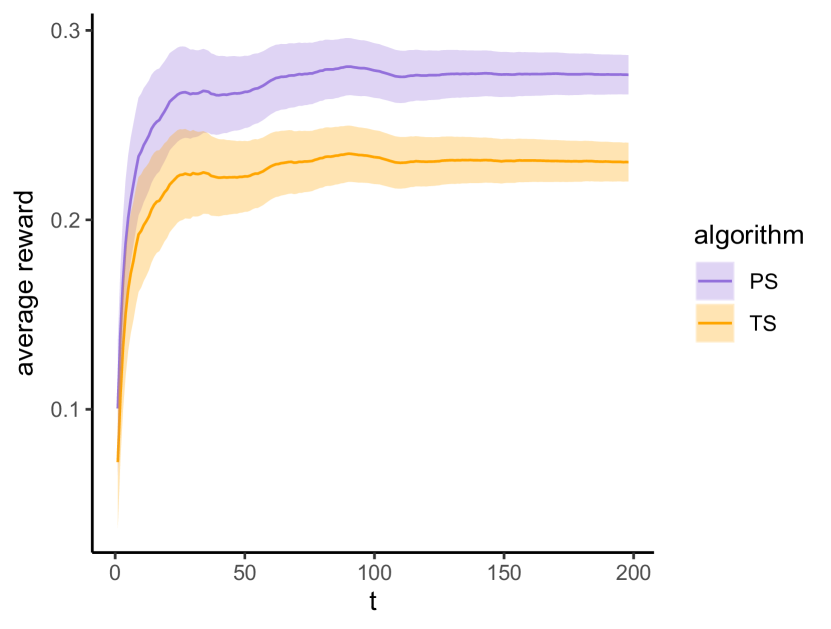
(b) Average Rewards

Figure 11: Experiment where $\eta=0.9$, and $t\in\{1,2,...,200\}$: (a) The frequencies at which Thompson sampling (TS) and predictive sampling (PS) agents select greedy actions. PS consistently selects greedy actions more than TS throughout time. (b) Average reward collected by TS and PS agents. PS consistently attains average reward higher than TS throughout time.

(a) Greedy Action Selection Frequencies

(b) Average Rewards

Figure 12: Experiment where $\eta\in\{0.1,0.3,0.5,0.7,0.9\}$, and $t=200$: (a) The frequencies at which Thompson sampling (TS) and predictive sampling (PS) agents select greedy actions. PS consistently selects greedy actions more than TS for varying $\eta$, and the gap between the greedy action selection frequencies increases as $\eta$ decreases. (b) Average reward collected by TS and PS agents. PS consistently attains average reward higher than TS for varying $\eta$, and the gap between the average rewards increases as $\eta$ decreases.

6.3 Continual Learning from Delayed Consequences

So far, we have considered supervised learning and bandit learning, both of which involve no delayed consequences. Indeed, the reward is immediate, and the agent’s actions have no influence on future situational states. In contrast, in this section we will consider the case in which actions have delayed consequences. Common examples of this include robotics, game playing (Go, chess, Hanabi, etc), and of course, regular life. In these cases, the agent’s actions affect which situations it ends up in, and the reward is often delayed. In our framing, we say that an agent’s actions affect future situational states, and the agent experiences delayed rewards. While our framing of “reinforcement learning” is very broad, we should note that it is precisely this problem formulation with delayed consequences that typically goes under the reinforcement learning rubric.

Most commonly, this problem is framed as learning in a Markov Decision Process (MDP). Typically, the MDP is stationary and not changing over time. To study continual learning, we will instead consider an MDP that is changing over time. In summary, we consider learning from delayed consequences in a nonstationary Markov Decision Process as a special case of our computationally constrained RL framework for continual learning. This type of environment has been extensively studied in prior work, surveyed by Padakandla [2021].

Environment

Consider an environment $\mathcal{E}=(\mathcal{A},\mathcal{O},\rho)$ in which observations are generated by a Markov decision process (MDP) with time-varying transition probabilities. Each observation $O_{t}$ is of the current state $S_{t}$ of the MDP. Hence, the state space of the MDP is $\mathcal{S}=\mathcal{O}$. We consider a small MDP where $\mathcal{S}=10$ and $\mathcal{A}=3$.

For each state-action pair $(s,a)$, the vector $(P_{t,s,a,s^{\prime}}:s^{\prime}\in\mathcal{S})$ represents the transition probabilities at time $t$. The initial transition probability vectors are independently sampled from a $\text{Dirichlet}(1/\mathcal{S},\ldots,1/\mathcal{S})$ distribution. At every time step $t$, the MDP is updated with some small probability. Specifically, for each state-action pair $(s,a)$, with some probability $\eta\in(0,1)$, the vector $(P_{t,s,a,s^{\prime}}:s^{\prime}\in\mathcal{S})$ is replaced by a new, independent $\text{Dirichlet}(1/\mathcal{S},\ldots,1/\mathcal{S})$ sample.

After the action $A_{t}$ is executed, the environment produces as an observation the next state $S_{t+1}=O_{t+1}$. This state is generated as though the environment samples from the state distribution $P_{t,S_{t},A_{t},\cdot}$. Note that this probability vector is random, and the deterministic observation probability function $\rho$ that characterizes environment dynamics is defined by

$$\rho(o|H_{t},A_{t})=\mathbb{E}[P_{t,S_{t},A_{t},o}|H_{t},A_{t}]$$

for all $o\in\mathcal{O}$.

There is a known distinguished state $s_{*}\in\mathcal{S}$, which we will refer to as the goal state. A nonzero reward is received only upon arrival at the goal state:

$$R_{t+1}=r(H_{t},A_{t},O_{t+1})=\left\{\begin{array}[]{ll}r_{t+1}>0&\text{if }S_{t+1}=s_{*}\\ 0&\text{otherwise.}\end{array}\right.$$

Because the MDP is changing over time, we can think of the agent as encountering different stationary MDPs (determined by $P_{t}$) throughout time. We scale the reward $r_{t+1}$ such that the optimal long-term average reward in each MDP is the same ($.5$). This ensures low variance across time and seeds. See details in Appendix C.2.

Agent

We consider the version of Q-learning introduced in Example 5 known as optimistic Q-learning. The agent is initialized with $Q_{0}(s,a)=0$ for all $(s,a)$ and updates action values according to

$$Q_{t+1}(s,a)=\left\{\begin{array}[]{ll}Q_{t}(S_{t},A_{t})+\alpha\left(R_{t+1}+\gamma\max_{a\in\mathcal{A}}Q_{t}(S_{t+1},a)-Q_{t}(S_{t},A_{t})\right)+\zeta&\text{if }(s,a)=(S_{t},A_{t})\\ Q_{t}(s,a)+\zeta&\text{otherwise.}\end{array}\right.$$

There are three hyperparameters: the stepsize $\alpha$, the discount factor $\gamma$, and the optimistic boost $\zeta$. The formula is identical to the regular Q-learning formula, with one addition: all action values are incremented with an optimistic boost $\zeta$ at each time step. This ensures that all actions will eventually be taken upon a revisit to a state. A higher $\zeta$ can be interpreted as leading to more exploration since it leads to all actions being revisited more often.

At each time step, the agent acts greedily with respect to $Q_{t}$ and selects the action with the highest action value. If multiple actions have the same action value the agent samples uniformly from those. Thus, $Q_{t}$ induces a mapping from situational state to action.

In the stationary setting with a constant MDP, there is an optimal action-value function $Q_{t}^{*}$ that does not change over time. Therefore, by annealing the stepsize and optimistic boost appropriately, the agent can converge on the optimal action-value function. The difference $|Q_{t}-Q_{t}^{*}|$ vanishes. By acting greedily to the optimal action-value function, the agent can perform optimally. In contrast, in our environment the MDP is changing at a constant rate and so is the associated optimal action-value function $Q_{t}^{*}$. In this case, annealing the stepsize and optimistic boost will result in premature convergence and hurt performance. By annealing the stepsize and optimistic boost, it will eventually update $Q_{t}$ at a much slower rate than the optimal action-value function $Q_{t}^{*}$ is changing. Indeed, the agent will update at a slower and slower rate, such that it effectively stops learning information that is useful: by the time the agent has made even a single update to $Q_{t}$, the optimal action-value function has changed many times over. Because the objective is the infinite-horizon average reward, any performance up until a finite time will have no influence on the overall long-term average reward. Thus, since an annealing agent will effectively stop learning after a certain point in time, it will underperform under the long-term average reward objective. This is generally true in the continual learning setting where the optimal mapping from situational state to action keeps changing indefinitely.

Consequently, in our experiments, we only consider constant $\alpha$ and $\zeta$ values. In reinforcement learning, the discount factor $\gamma$ is typically presented as a component of the MDP. In our framing of continual learning, $\gamma$ is instead a hyperparameter of the agent that controls the effective planning horizon. For all experiments, we set $\gamma=0.9$.

Results

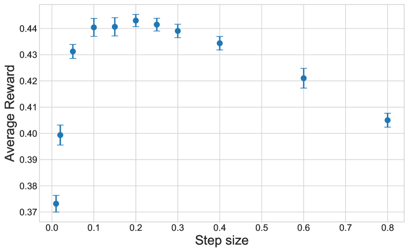
(a) $\eta=1e-4$

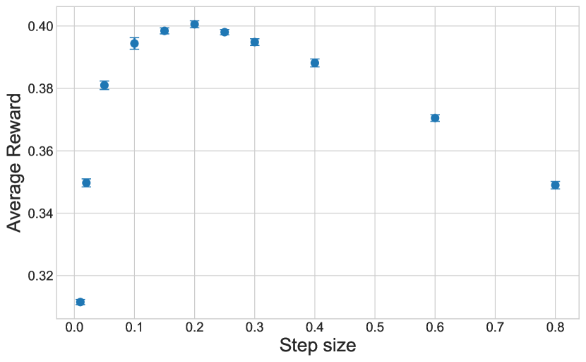
(b) $\eta=1e-3$

Figure 13: Average reward versus the stepsize $\alpha$. Interestingly, optimal stepsize is the same ($.2$) in both environments.

(a) $\eta=1e-4$

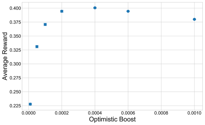
(b) $\eta=1e-3$

Figure 14: Average reward versus the optimistic boost $\zeta$. As the nonstationarity parameter $\eta$ increases, the optimal optimistic boost $\zeta^{*}$ increases.

On each environment, we perform a sweep over stepsize $\alpha$ and optimistic boost $\zeta$ to select the optimal values. On each environment, we plot how the average reward depends on the stepsize $\alpha$ and optimistic boost $\zeta$, respectively. For each value of $\alpha$, in Figure 13, we plot the largest average reward achievable when sweeping over $\zeta$. Similarly, in Figure 14, we plot the largest average reward achievable for each $\zeta$. We find that the optimal optimistic boost increases with the degree of nonstationarity in the environment. These results are intuitive. When the environment is changing, old knowledge becomes obsolete, and it is imperative to seek out new knowledge. Higher values of optimistic boost lead to more exploratory behavior needed to accomplish this. In contrast, however, we note that it is a little surprising that the optimal stepsize was the same in both environments.

In more complex environments, it is cumbersome or infeasible to perform a hyperparameter search to find optimal values. We conjecture that a more sophisticated agent, without being initialized with the optimal hyperparameters, could automatically learn them over time, fully online. This is an example of meta-learning which has been explored extensively in previous literature (see e.g Duan et al. [2016], Flennerhag et al. [2021], Thrun and Pratt [1998]). Because our objective considers an infinite horizon, the sophisticated agent would therefore be able to reach the same asymptotic performance as an agent that is initialized with the optimal hyperparameters.

6.4 Continual Auxiliary Learning

While an agent’s goal is to maximize average reward, a complex environment can offer enormous amounts of feedback beyond reward. This feedback can be used to accelerate the agent’s learning and thus increase its average reward. For example, sensors of a self-driving car ingest visual and auditory feedback far beyond what is required to determine reward, which, for example, might simply indicate safe arrival to a destination. By predicting future trajectories of its own vehicle, learning from realizations to improve these predictions, and using these predictions to plan, an agent can learn to maximize reward much more quickly than if it learned only from reward feedback.

Auxiliary tasks that are those distinct from, though possibly helpful to, the primary task of maximizing average reward. Prediction of future outcomes other than reward, as we considered in our self-driving car example, serves as an example of an auxiliary task. Learning to perform auxiliary tasks can accelerate learning for the primary task.

In a complex environment, it is often unclear what auxiliary tasks are helpful and how they relate to the primary task. However, a long-lived agent can learn that over time. We refer to this continual auxiliary learning. In the remainder of this section, we illustrate benefits of continual auxiliary learning through the following didactic example:

Example 12.

(continual auxiliary learning) Consider a modified version of continual SL where the input set is the singleton $\mathcal{X}=\{\emptyset\}$, and the label set consists of $k$ dimensional binary vectors $\mathcal{Y}=\{0,1\}^{k}$. The labels are generated via

$$Y_{t+1}\sim\sigma(\phi_{t}),$$

where $\sigma$ denotes the sigmoid function $\exp(x)/(1+\exp(x))$ applied element-wise. We assume that $\phi_{t}=A\theta_{t}$, where $A$ is a sparse vector with only $K$ non-zero components (including the first), and $\theta_{t}\in\Re$ evolves according to the AR(1) process

$$\theta_{t}=\eta\theta_{t-1}+W_{t},$$

where $W_{t}\overset{iid}{\sim}\mathcal{N}(0,1-\eta^{2})$ and $W_{t}\perp\theta_{t-1}$. The actions of the agent are predictions about the first component $Y_{t+1,1}$ of the label. Hence, $\mathcal{A}=\Delta_{\{0,1\}}$. We take reward to be the negative log-loss:

$$r(H_{t},A_{t},O_{t+1})=\ln P_{t}(Y_{t+1,1}).$$

In this example, prediction of $Y_{t+1,1}$ constitutes the primary task. Prediction of the remaining label components $Y_{t+1,2:k}$ are possible auxiliary tasks. These components may offer information that allows an agent to more quickly learn about $\theta_{t}$, which in turns improves its ability to perform its primary task. If there the number of components $k$ is large and most components are not relevant to the agent’s primary task, a long-lived agent can improve its performance by learning which components are relevant. In particular, an agent can learn over time about the vector $A$. Learning about $A$ enhances the agent’s ability to quickly learn about $\theta_{t}$. Learning about $A$ can be thought of as meta-learning, as it aims to learn about something that can guide the agent’s learning about its primary task. In the following sections, we will investigate performance gains that this affords.

6.4.1 Methods

No auxiliary learning

As a baseline, we consider an agent that ignores all auxiliary components$Y_{t+1,2:k}$. The agent maintains a vector $\hat{\phi}_{t}\in\Re$. At each time, it first scales $\hat{\phi}_{t}$ by $\mu$ and then updates the vector via gradient descent to maximize reward:

$$\hat{\phi}_{t}^{\prime} =\mu\hat{\phi}_{t}$$

$$L_{t} =-Y_{t+1,1}\log(\sigma(\hat{\phi}_{t}^{\prime}))-(1-Y_{t+1,1})\log(1-\sigma(\hat{\phi}_{t}^{\prime}))$$

$$g_{t} =\frac{\partial}{\partial{\hat{\phi}_{t}^{\prime}}}L_{t}$$

$$=\frac{-Y_{t+1,1}+(1-Y_{t+1,1})\exp(\hat{\phi}_{t}^{\prime})}{1+\exp(\hat{\phi}_{t}^{\prime})}$$

$$\hat{\phi}_{t+1} =\hat{\phi}_{t}^{\prime}-\alpha g_{t},$$

where the best learning rate $\alpha$ is found by grid search.

Auxiliary learning with $A$ known

We also consider the agent that perfectly learns from the auxiliary information. In particular, consider the agent that is given the value of $A$, and maintains $\hat{\theta}_{t}\in\Re$. At each time step, it first decays $\hat{\theta}_{t}$ by $\mu$, and then updates it by gradient descent to minimize the loss with respect to all components of $Y$:

$$\hat{\theta}_{t}^{\prime} =\mu\hat{\theta}_{t}$$

$$L_{t} =-Y_{t+1}^{T}\log(\sigma(A\hat{\theta}_{t}^{\prime}))-(1-Y_{t+1})^{T}\log(1-\sigma(A\hat{\theta}_{t}^{\prime}))$$

$$g_{t} =\frac{\partial}{\partial{\hat{\theta}_{t}^{\prime}}}L_{t}$$

$$=A^{T}\left[\left(-Y_{t+1}+(1-Y_{t+1})\odot\exp(A\hat{\theta}_{t}^{\prime})\right)\oslash\left(1+\exp(A\hat{\theta}_{t}^{\prime})\right)\right]$$

$$\hat{\theta}_{t+1} =\hat{\theta}_{t}^{\prime}-\alpha g_{t},$$

where we use $\odot$ and $\oslash$ to denote element-wise multiplication and division, respectively, and the best learning rate $\alpha$ is found by grid search.

Auxiliary learning with $A$ learned

This agent internally maintains both $\hat{A}_{t}$ and $\hat{\theta}_{t}$. It uses vanilla gradient descent on the loss with respect to all components to update $\hat{\theta}_{t}$, and learns $\hat{A}_{t}$ via meta gradient descent. The update rules for $\theta_{t}$ are

$$\hat{\theta}_{t}^{\prime} =\mu\hat{\theta}_{t}$$

$$L_{t} =-Y_{t+1}^{T}\log(\sigma(\hat{A}_{t}\hat{\theta}_{t}^{\prime}))-(1-Y_{t+1})^{T}\log(1-\sigma(\hat{A}_{t}\hat{\theta}_{t}^{\prime}))$$

$$g_{t} =\frac{\partial}{\partial{\hat{\theta}_{t}^{\prime}}}L_{t}$$

$$=\hat{A}_{t}^{T}\left[\left(-Y_{t+1}+(1-Y_{t+1})\odot\exp(\hat{A}_{t}\hat{\theta}_{t}^{\prime})\right)\oslash\left(1+\exp(\hat{A}_{t}\hat{\theta}_{t}^{\prime})\right)\right]$$

$$\hat{\theta}_{t+1} =\hat{\theta}_{t}^{\prime}-\alpha g_{t},$$

and the update rules for $\hat{A}_{t}$ are

$$h_{t} =\mu h_{t-1}-\alpha\mu\left(-Y_{t}+(1-Y_{t})\odot\exp(\hat{A}_{t-1}\hat{\theta}_{t-1}^{\prime})\right)\oslash\left(1+\exp(\hat{A}_{t-1}\hat{\theta}_{t-1}^{\prime})\right)$$

$$\qquad\qquad-\alpha\mu\hat{A}_{t-1}^{T}\left[\exp(\hat{A}_{t-1}\hat{\theta}_{t-1}^{\prime})\odot\hat{A}_{t-1}\oslash\left(1+\exp(\hat{A}_{t-1}\hat{\theta}_{t-1}^{\prime})\right)^{\circ 2}\right]h_{t-1}$$

$$\hat{A}_{t+1} =\hat{A}_{t}-\beta g_{t}h_{t},$$

where $A^{\circ 2}$ denotes element-wise square of $A$, and $\beta$ is the meta-learning rate. Readers are referred to Appendix C.3 for derivation of these update rules.

6.4.2 Results

Figure 15 plots reward versus time. The results are generated with autoregressive model coefficient $\mu=0.99$ and label dimension $k=100$, $K=10$ useful components. For the agent with no auxiliary learning and the agent performing auxiliary learning with $A$ known, the best learning rate $\alpha$ found by grid search is used ($0.202$ and $0.092$, respectively). The agent performing auxiliary learning with $A$ learned uses a learning rate $\alpha=0.01$, which is far from optimal, and a meta-learning rate $\beta=0.05$.

Figure 15: Learning $A$ eventually yields performance at the level attained if $A$ were known. This exceeds the performance of an agent that does not engage in auxiliary learning.

From Figure 15 we can see that learning $A$ eventually yields performance at the level achieved with $A$ known. Either of these outperform an agent that does not engage in auxiliary learning. This demonstrates how continual auxiliary learning can help an agent perform well in the long run, even if the agent does not initially know what auxiliary tasks are useful.

However, the performance improvement comes at the cost of extra computation. In this particular example, the agent that does not engage in auxiliary learning requires $O(1)$ FLOPs per time step, while the others require $O(k)$ FLOPs per time step. Hence, the performance improvement relies on roughly $k$ times more compute. In the general case, implementing continual auxiliary learning in a scalable manner, with only a modest increase in compute, remains an interesting topic for future research.

Summary

Continual Supervised Learning

• We consider continual supervised learning with an objective of maximizing average online accuracy:

  $$\begin{array}[]{ll}\max_{\pi}&\liminf_{T\rightarrow\infty}\mathbb{E}_{\pi}\left[\frac{1}{T}\sum_{t=0}^{T-1}\mathbbm{1}(Y_{t+1}=\hat{Y}_{t+1})\right]\\ \text{s.t.}&\text{computational constraint}\end{array}$$

• Evaluation Protocol: we first tune hyperparameters on a development sequence and then train the agent with the best hyperparameters on multiple evaluation sequences. The agent’s performance is averaged across all evaluation sequences.

• Experiments with a variant of permuted MNIST indicate that:

  • A performant agent can forget non-recurring information.

  • A performant agent can forget recurring information if it can relearn that information quickly relative to the duration of the information’s utility.

  • When computation is constraining, forgetting can increase average reward.

Continual Exploration

• Via experiments with a coin swapping game, we identify three properties of effective exploration in the face of nonstationarity:

  • An optimal agent never stops exploring.

  • An agent should prioritize acquisition of more durable information – that is, information that will remain valuable and relevant over a longer duration.

  • To assess durability of information, an agent can benefit from learning about environment dynamics.

• Via experiments with a two-armed Gaussian bandit, we demonstrate that prioritizing acquisition of more durable information is beneficial for maximizing average reward and that the benefit of this is greater in environments with less durable information.

Continual Learning with Delayed Consequences

• Optimistic Q-learning can learn from delayed consequences in a nonstationary Markov decision processes.

• As the degree of nonstationarity increase, more intense exploration increases average reward.

• A more sophisticated agent may be able to adapt stepsize, discount, and optimism hyperparameters online to increase average reward.

Continual Auxiliary Learning

• Auxiliary tasks are tasks that are those distinct from, though possibly helpful to, the primary task of maximizing average reward.

• Auxiliary learning refers to identifying useful auxiliary tasks and their relationship to the primary task.

• A long-lived agent has time to learn not only how to perform auxiliary tasks but also what auxiliary tasks are useful to learn about and how they relate to the primary task.

7 Conclusion

Summary. In this paper, we framed continual learning as computationally constrained reinforcement learning. Under this perspective, we formally introduced an objective for continual learning. This objective is to maximize the infinite-horizon average reward under computational constraints. We formalized the concepts of agent state, information capacity, and learning targets, which play key roles for thinking about continual learning and distinguishing it from traditional vanishing-regret learning. Leveraging information theory, we decomposed prediction error into forgetting and implasticity components. We concluded with case studies that studied implications of our objective on behaviors of performant agents.

Future Research. In our case studies, we discussed how different agent capabilities contribute to performance under our objective. These capabilities include balancing forgetting with fast relearning, seeking out durable information when exploring, modeling environment dynamics, and meta-learning hyperparameters. We hope that this work inspires researchers to design agents that exhibit such capabilities and to study the trade-offs between them under computational constraints. In particular, we hope our holistic objective helps researchers reason about these trade-offs and reveal additional desired capabilities.

Appendix

Appendix A MDP Exchangeability

This section presents conditions under which it is natural to characterize dynamics using an unknown MDP, in other words, characterizing the environment as a mixture of MDP. Suppose each observation is interpreted as a situational state $S_{t}=O_{t}$ and rewards depend on history only through the situational state, taking the form $R_{t+1}=r(S_{t},A_{t},S_{t+1})$. The environment is a mixure of MDP, if there exists a random variable $P$, where each $P_{a}$ is a $|\mathcal{S}|\times|\mathcal{S}|$ stochastic transition matrix with $P_{sas^{\prime}}$ denoting its $(s,s^{\prime})$ entry, such that for all policies $\pi$, time $T\in\mathbb{Z}_{+}$, and histories $h_{T}=(a_{0},s_{1},a_{1},s_{2},...,a_{T-1},s_{T})\in\mathcal{H}_{T}$, we have

$$\mathbb{P}_{\pi}(H_{T}=h_{T}|P)=\prod_{t=0}^{T-1}P_{s_{t}a_{t}s_{t+1}}\prod_{t=0}^{T-1}\pi(a_{t}|h_{t}),$$ (15)

where $h_{t}=(a_{0},s_{1},a_{1},s_{2},...,a_{t-1},s_{t})$. This $P$ represents a natural learning target in this case.

We assume that a recurrent-like property holds. Specifically, let $\overline{\pi}$ be defined such that $\overline{\pi}(a|h)=1/|\mathcal{A}|$ for all $a\in\mathcal{A}$ and $h\in\mathcal{H}$, we assume that

$$\mathbb{P}_{\overline{\pi}}\left(S_{t}=S_{1}\text{ for infinitely many }t\right)=1.$$ (16)

We introduce a certain kind of symmetry condition on the set of all histories. Specifically, we introduce a binary relation $\sim$. Let $h,h^{\prime}\in\mathcal{H}$ be two histories of finite horizon. We let $h\sim h^{\prime}$ if and only if they exhibit the same number of state-action-state transition counts, for every such state-action-state tuple. Here, we assume that $S_{0}$ is deterministic and $S_{t}\neq S_{0}$ a.s. for all $t\in\mathbb{N}_{++}$. For instance, let $\mathcal{S}=\mathbb{N}$, and $\mathcal{A}=\{a,b,c,d\}$, $x2y3\nsim x3y2$ but $x2y1x3z2\sim x3z2y1x2$.

We establish a theorem, which extends partial exchangeability established by Diaconis and Freedman [1980]. The theorem provides a necessary and sufficient condition for the environment to be a mixture of MDP.

Theorem 6.

Suppose Equation 16 holds. Then the environment is a mixture of MDP in the sense of Equation 15 if and only if for all policies $\pi$ and $\pi^{\prime}$, all $T\in\mathbb{Z}_{+}$, and all histories $h_{T},h^{\prime}_{T}\in\mathcal{H}_{T}$,

$$h_{T}\sim h_{T}^{\prime}\quad\mathrm{implies}\quad\frac{\mathbb{P}_{\pi}(H_{T}=h_{T})}{\prod_{t=0}^{T-1}\pi(a_{t}|h_{t})}=\frac{\mathbb{P}_{\pi^{\prime}}(H_{T}=h_{T}^{\prime})}{\prod_{t=0}^{T-1}\pi^{\prime}{(a_{t}^{\prime}|h_{t}^{\prime})}}.$$

Proof.

The “$\Rightarrow$” direction is obvious. We prove the other direction. Let $\overline{\pi}$ be defined such that $\overline{\pi}(a|h)=\frac{1}{|\mathcal{A}|}$ for $a\in\mathcal{A}$ and $h\in\mathcal{H}$. For any two histories $h_{T},h^{\prime}_{T}\in\mathcal{H}_{T}$ for all $T\in\mathbb{Z}_{+}$, if the state-action-state-action transition counts in $h_{T}$ and $h^{\prime}_{T}$ are the same for all state-action-state-action tuples (we assume that the last action is the same), then $h_{T}\sim h^{\prime}_{T}$. This implies that

$$\frac{\mathbb{P}_{\overline{\pi}}(H_{T}=h_{T})}{\prod_{t=0}^{T-1}\overline{\pi}(a_{t}|h_{t})}=\frac{\mathbb{P}_{\overline{\pi}}(H_{T}=h_{T}^{\prime})}{\prod_{t=0}^{T-1}\overline{\pi}(a_{t}^{\prime}|h_{t}^{\prime})}.$$

Hence, $\mathbb{P}_{\overline{\pi}}(H_{T}=h_{T})=\mathbb{P}_{\overline{\pi}}(H_{T}=h_{T}^{\prime})$.

By Theorem 7 of [Diaconis and Freedman, 1980], $X_{t}=(S_{t},A_{t})$, defined by $\overline{\pi}$, is a mixture of Markov chains. In other words, there exists a $|\mathcal{S}||\mathcal{A}|\times|\mathcal{S}||\mathcal{A}|$ stochastic transition matrix-valued random variable $\overline{P}$, where each element in the $(sa,s^{\prime}a^{\prime})$-th position is denoted by $\overline{P}_{sa,s^{\prime}a^{\prime}}$, such that for all $T\in\mathbb{Z}_{+}$ and history $h\in\mathcal{H}_{T}$,

$$\mathbb{P}_{\overline{\pi}}\left(H_{T}=h_{T}|\overline{P}\right)=\prod_{t=0}^{T-1}\overline{P}_{s_{t}a_{t},s_{t+1}a_{t+1}}.$$

We define $P$ as follows: for all $s,s^{\prime}\in\mathcal{S}$ and $a\in\mathcal{A}$, we have

$$P_{sas^{\prime}}=\sum_{a^{\prime}\in\mathcal{A}}\overline{P}_{sa,s^{\prime}a^{\prime}},$$

(or, equivalently, $P_{sas^{\prime}}=|\mathcal{A}|\overline{P}_{sa,s^{\prime}a^{\prime}}$ for any $a^{\prime}\in\mathcal{A}$). Then, for all policies $\pi$, all $T\in\mathbb{Z}_{+}$ and all $h_{T}\in\mathcal{H}_{T}$,

$$\mathbb{P}_{\pi}(H_{T}=h_{T}|P)=\frac{P_{\overline{\pi}}(H_{T}=h_{T}|P)}{\prod_{t=0}^{T-1}\overline{\pi}(a_{t}|h_{t})}\prod_{t=0}^{T-1}\pi(a_{t}|h_{t})=\prod_{t=0}^{T-1}P_{s_{t}a_{t}s_{t+1}}\prod_{t=0}^{T-1}\pi(a_{t}|h_{t}).$$

∎

When the environment is a mixure of MDP determined by $P$, the latent transition probabilities serve as a natural learning target $\chi=P$. The “efficient reinforcement learning” literature presents many agents and analyses that treat $P$ as a learning target.

Appendix B Capacity-Constrained LMS with an AR(1) Process

In this section we provide a detailed analysis of the didactic example discussed in 5.2. In B.1 we introduce a reparameterization of the agent update rule in Equation 13, and derive some useful formulas, including the posterior predictions of the agent (Theorem 11). We then apply these formulas to calculate the implasticity error and forgetting error (B.2).

B.1 Reparameterizing the Agent

In this section we offer a reparameterization of the update rule in Equation 13, and derive some useful formulas. We let ${\alpha^{\prime}}=1-\alpha$. Then, Equation 13 can be rewritten as

$$U_{t+1}={\alpha^{\prime}}U_{t}+\alpha Y_{t+1}+Q_{t+1}.$$ (17)

In the results to follow, we derive closed form expressions for $U_{t}$ and $Y_{t+1}$ in terms of independent Gaussian random variables. Doing so will allow us derive exact formulas for relevant information-theoretic quantities.

We begin by deriving a closed form formula for $U_{t}$ in terms of independent Gaussian random variables:

Lemma 7.

For all $t\in\mathbb{Z}_{++}$,

$$U_{t}=\sum_{i=0}^{t-1}\alpha{\alpha^{\prime}}^{i}W_{t-i}+\sum_{i=0}^{t-1}\alpha\frac{\eta^{i}-{\alpha^{\prime}}^{i}}{\eta-{\alpha^{\prime}}}V_{t-i}+\alpha\frac{\eta^{t}-{\alpha^{\prime}}^{t}}{\eta-{\alpha^{\prime}}}\theta_{0}+{\alpha^{\prime}}^{t}U_{0}+\sum_{i=0}^{t-1}{\alpha^{\prime}}^{i}Q_{t-i},$$

where we set $\frac{\eta^{i}-{\alpha^{\prime}}^{i}}{\eta-{\alpha^{\prime}}}=i\eta^{i-1}$ when $\eta={\alpha^{\prime}}$.

Proof.

The base case $(t=0)$ can trivially be verified. The cases where $t\geq 1$ can be proven by induction, by directly plugging in the formula. ∎

We now provide analogous formulas for $\theta_{t}$ and $Y_{t+1}$.

Lemma 8.

For all $t\in\mathbb{Z}_{++}$,

$$\theta_{t}=\sum_{i=0}^{t-1}\eta^{i}V_{t-i}+\eta^{t}\theta_{0}.$$

Corollary 9.

For all $t\in\mathbb{Z}_{++}$

$$Y_{t+1}=\sum_{i=0}^{t-1}\eta^{i}V_{t-i}+\eta^{t}\theta_{0}+W_{t+1}.$$

We omit the proofs as they all follow from simple applications of induction.

As we are interested in the steady state behavior of error, the following lemma provides closed-form expressions for quantities which comprise the covariance matrices relevant for forgetting and implasticity error computations.

Lemma 10.

As $t\to\infty$,

$$\mathbb{E}[Y_{t}^{2}] =1+\sigma^{2},$$

$$\mathbb{E}[Y_{t}Y_{t+k}] =\eta^{k}\qquad\forall k\geq 1,$$

$$\mathbb{E}[U_{t}^{2}] =\frac{\alpha^{2}\sigma^{2}}{1-{\alpha^{\prime}}^{2}}+\frac{\alpha^{2}(1-\eta^{2})}{(\eta-{\alpha^{\prime}})^{2}}\left(\frac{1}{1-\eta^{2}}+\frac{1}{1-{\alpha^{\prime}}^{2}}-\frac{2}{1-\eta{\alpha^{\prime}}}\right)+\frac{\delta^{2}}{1-{\alpha^{\prime}}^{2}}$$

$$=\alpha\frac{\sigma^{2}(1-{\alpha^{\prime}}\eta)+1+{\alpha^{\prime}}\eta}{(1-{\alpha^{\prime}}\eta)(1+{\alpha^{\prime}})}+\frac{\delta^{2}}{1-{\alpha^{\prime}}^{2}},$$

$$\mathbb{E}[U_{t}U_{t+1}] =\frac{\alpha^{2}\sigma^{2}{\alpha^{\prime}}}{1-{\alpha^{\prime}}^{2}}+\frac{\alpha^{2}(1-\eta^{2})}{(\eta-{\alpha^{\prime}})^{2}}\left(\frac{\eta}{1-\eta^{2}}+\frac{{\alpha^{\prime}}}{1-{\alpha^{\prime}}^{2}}-\frac{\eta+{\alpha^{\prime}}}{1-\eta{\alpha^{\prime}}}\right)+\frac{{\alpha^{\prime}}\delta^{2}}{1-{\alpha^{\prime}}^{2}}$$

$$=\alpha\frac{{\alpha^{\prime}}\sigma^{2}(1-{\alpha^{\prime}}\eta)+{\alpha^{\prime}}+\eta}{(1-{\alpha^{\prime}}\eta)(1+{\alpha^{\prime}})}+\frac{{\alpha^{\prime}}\delta^{2}}{1-{\alpha^{\prime}}^{2}},$$

$$\mathbb{E}[U_{t+k}Y_{t}] =\alpha\sigma^{2}{\alpha^{\prime}}^{k}+\frac{\alpha(1-\eta^{2})}{\eta-{\alpha^{\prime}}}\left(\frac{\eta^{k+1}}{1-\eta^{2}}-\frac{{\alpha^{\prime}}^{k+1}}{1-\eta{\alpha^{\prime}}}\right)\qquad\forall k\geq 0$$

$$=\alpha\sigma^{2}{\alpha^{\prime}}^{k}+\frac{\alpha}{1-\eta{\alpha^{\prime}}}\left(\frac{\eta^{k+1}-{\alpha^{\prime}}^{k+1}}{\eta-{\alpha^{\prime}}}-\eta^{2}{\alpha^{\prime}}\frac{\eta^{k}-{\alpha^{\prime}}^{k}}{\eta-{\alpha^{\prime}}}\right),$$

$$\mathbb{E}[U_{t}Y_{t+k}] =\frac{\alpha\eta^{k-1}(1-\eta^{2})}{\eta-{\alpha^{\prime}}}\left(\frac{1}{1-\eta^{2}}-\frac{1}{1-\eta{\alpha^{\prime}}}\right)\qquad\forall k\geq 1$$

$$=\frac{\alpha\eta^{k}}{1-{\alpha^{\prime}}\eta}.$$

For the remainder of the analysis, we will assume that $U_{t}$ and $Y_{t}$ are weak-sense jointly stationary processes with covariance given by the previous expressions. Since $U_{t}$ and $Y_{t}$ are jointly Gaussian, this implies that they are strong-sense jointly stationary as well.

With the expressions derived in Lemma 10, we now provide the steady state posterior distribution of $Y_{t+1}$ conditioned on $U_{t}$. Recall that this posterior distribution constitutes the optimal prediction of $Y_{t+1}$ conditioned on $U_{t}$.

Theorem 11.

(posterior predictions)

$$\lim_{t\to\infty}\mathbb{P}(Y_{t+1}\in\cdot|U_{t})=\mathcal{N}\left(\mu,\ \Delta^{2}\right),$$

where

$$\mu=\frac{\alpha\eta(1-{\alpha^{\prime}}^{2})}{\alpha^{2}\sigma^{2}(1-{\alpha^{\prime}}\eta)+\alpha^{2}(1+{\alpha^{\prime}}\eta)+\delta^{2}(1-{\alpha^{\prime}}\eta)}U_{t}$$

and

$$\Delta^{2}=1+\sigma^{2}-\frac{\alpha^{2}\eta^{2}(1-{\alpha^{\prime}}^{2})}{\alpha^{2}\sigma^{2}(1-{\alpha^{\prime}}\eta)^{2}+\alpha^{2}(1-{\alpha^{\prime}}^{2}\eta^{2})+\delta^{2}(1-{\alpha^{\prime}}\eta)^{2}}.$$

Proof.

Since all the variables are $0$-mean multivariate Gaussians, $Y_{t+1}$ is a Gaussian conditioned on $U_{t}$. Its mean is given by

$$\mathbb{E}[Y_{t+1}|U_{t}] =\frac{\mathbb{E}[U_{t}Y_{t+1}]}{\mathbb{E}[U_{t}^{2}]}U_{t}$$

$$=\frac{\frac{\alpha\eta}{1-{\alpha^{\prime}}\eta}}{\alpha^{2}\frac{\sigma^{2}(1-{\alpha^{\prime}}\eta)+1+{\alpha^{\prime}}\eta}{(1-{\alpha^{\prime}}\eta)(1-{\alpha^{\prime}}^{2})}+\frac{\delta^{2}}{1-{\alpha^{\prime}}^{2}}}U_{t}$$

$$=\frac{\alpha\eta(1-{\alpha^{\prime}}^{2})}{\alpha^{2}\sigma^{2}(1-{\alpha^{\prime}}\eta)+\alpha^{2}(1+{\alpha^{\prime}}\eta)+\delta^{2}(1-{\alpha^{\prime}}\eta)}U_{t},$$ (18)

and its variance is given by

$$\mathbb{V}[Y_{t+1}|U_{t}] =\mathbb{E}[Y_{t+1}^{2}]-\frac{\mathbb{E}[U_{t}Y_{t+1}]^{2}}{\mathbb{E}[U_{t}^{2}]}$$

$$=1+\sigma^{2}-\frac{\left(\frac{\alpha\eta}{1-{\alpha^{\prime}}\eta}\right)^{2}}{\alpha^{2}\frac{\sigma^{2}(1-{\alpha^{\prime}}\eta)+1+{\alpha^{\prime}}\eta}{(1-{\alpha^{\prime}}\eta)(1-{\alpha^{\prime}}^{2})}+\frac{\delta^{2}}{1-{\alpha^{\prime}}^{2}}}$$

$$=1+\sigma^{2}-\frac{\alpha^{2}\eta^{2}(1-{\alpha^{\prime}}^{2})}{\alpha^{2}\sigma^{2}(1-{\alpha^{\prime}}\eta)^{2}+\alpha^{2}(1-{\alpha^{\prime}}^{2}\eta^{2})+\delta^{2}(1-{\alpha^{\prime}}\eta)^{2}},$$ (19)

where we use the covariances calculated in Lemma 10. ∎

We now derive a closed-form solution to the value of $\delta^{2}$ (variance of quantization noise) which will ensure that agent state $U_{t}$ will contain at most $C$ nats of information about $H_{t}$ as $t\to\infty$.

Theorem 12.

(information capacity) For all $\alpha\in[0,1]$, the minimal quantization noise variance $\delta^{2}$ needed to achieve information capacity $C$, i.e.,

$$\limsup_{t\to\infty}\mathbb{I}(U_{t};H_{t})\leq C,$$

is given by

$$\delta^{2}=\alpha^{2}\frac{\sigma^{2}(1-{\alpha^{\prime}}\eta)+1+{\alpha^{\prime}}\eta}{1-{\alpha^{\prime}}\eta}\frac{\exp(-2C)}{1-\exp(-2C)}.$$

Proof.

We let $\Sigma$ denote the covariance matrix of $H_{t}=Y_{1:t}$ and the vector $\phi$ denote the covariance between $U_{t}$ and $Y_{1:t}$:

$$\phi=\begin{bmatrix}\mathbb{E}[U_{t}Y_{1}]&\mathbb{E}[U_{t}Y_{2}]&...&\mathbb{E}[U_{t}Y_{t}]\end{bmatrix}^{T}.$$

Since the variables are multivariate $0$-mean Gaussians, the mutual information is given by

$$\mathbb{I}(U_{t};H_{t}) =\frac{1}{2}\left(\log\mathbb{E}[U_{t}^{2}]+\log\det\Sigma-\log\det\begin{bmatrix}\mathbb{E}[U_{t}^{2}]&\phi^{T}\\ \phi&\Sigma\end{bmatrix}\right)$$

$$=\frac{1}{2}\left(\log\mathbb{E}[U_{t}^{2}]+\log\det\Sigma-\log\det\begin{bmatrix}\mathbb{E}[U_{t}^{2}]-\phi^{T}\Sigma^{-1}\phi&0\\ \phi&\Sigma\end{bmatrix}\right)$$

$$=\frac{1}{2}\left(\log\mathbb{E}[U_{t}^{2}]-\log\left(\mathbb{E}[U_{t}^{2}]-\phi^{T}\Sigma^{-1}\phi\right)\right)$$

$$=-\frac{1}{2}\log\left(1-\frac{\phi^{T}\Sigma^{-1}\phi}{\mathbb{E}[U_{t}^{2}]}\right).$$

From Lemma 10 we know that neither $\phi$ or $\Sigma$ depends on $\delta^{2}$. Hence, the above expression only depends on $\delta^{2}$ through

$$\mathbb{E}[U_{t}^{2}]=\alpha\frac{\sigma^{2}(1-{\alpha^{\prime}}\eta)+1+{\alpha^{\prime}}\eta}{(1-{\alpha^{\prime}}\eta)(1+{\alpha^{\prime}})}+\frac{\delta^{2}}{1-{\alpha^{\prime}}^{2}}.$$

For every positive $\delta$, $\mathbb{I}(U_{t};H_{t})=h(U_{t})-h(U_{t}|H_{t})$ is finite. As $\delta\to 0^{+}$, $h(U_{t})$ converges to a finite value, while $h(U_{t}|H_{t})$ diverges to negative infinity. This implies that when $\delta=0$,

$$\phi^{T}\Sigma^{-1}\phi=\mathbb{E}_{\delta=0}[U_{t}^{2}]=\alpha\frac{\sigma^{2}(1-{\alpha^{\prime}}\eta)+1+{\alpha^{\prime}}\eta}{(1-{\alpha^{\prime}}\eta)(1+{\alpha^{\prime}})}.$$

Note that $\mathbb{I}(U_{t};H_{t})\leq C$ is equivalent to

$$\mathbb{E}[U_{t}^{2}]\geq\frac{\phi^{T}\Sigma^{-1}\phi}{1-\exp(-2C)}=\frac{\mathbb{E}_{\delta=0}[U_{t}^{2}]}{1-\exp(-2C)}.$$

Plugging in the formula for $\mathbb{E}[U_{t}^{2}]$, we get

$$\delta^{2} \geq(1-{\alpha^{\prime}}^{2})\alpha\frac{\sigma^{2}(1-{\alpha^{\prime}}\eta)+1+{\alpha^{\prime}}\eta}{(1-{\alpha^{\prime}}\eta)(1+{\alpha^{\prime}})}\frac{\exp(-2C)}{1-\exp(-2C)}$$

$$=\alpha^{2}\frac{\sigma^{2}(1-{\alpha^{\prime}}\eta)+1+{\alpha^{\prime}}\eta}{1-{\alpha^{\prime}}\eta}\frac{\exp(-2C)}{1-\exp(-2C)}.$$

∎

B.2 Plasticity and Forgetting Error

Assuming $\{U_{t}\}$ and $\{Y_{t}\}$ are weak-sense jointly stationary processes, the total forgetting error can be simplified via Theorem 5 to be

$$\mathbb{I}(H_{t+1:\infty};U_{t-1}|U_{t},O_{t})=\mathbb{I}(Y_{t+1:\infty};U_{t-1}|U_{t},Y_{t}).$$

Similarly, the total implasticity error simplifies to

$$\mathbb{I}(H_{t+1:\infty};O_{t}|U_{t})=\mathbb{I}(Y_{t+1:\infty};Y_{t}|U_{t}).$$

All the variables in the above expressions are linear combinations of $0$ mean multivariate normal variables, and so they are also $0$ mean multivariate normal variables. Hence we can calculate this mutual information using the well known formula for conditional mutual information of multivariate Gaussians:

Lemma 13.

If $X_{1},X_{2},X_{3}$ are jointly Gaussian with covariance matrix $\Sigma_{123}$. Then,

$$\mathbb{I}(X_{1};X_{2}|X_{3})=\frac{1}{2}\ln\frac{\det\Sigma_{13}\det\Sigma_{23}}{\det\Sigma_{123}\det\Sigma_{3}},$$

where we use $\Sigma_{ij}$ and $\Sigma_{i}$ to denote submatrices corresponding to the respective variables $X_{i}$.

We can use the covariances in Lemma 10 to calculate these determinants.

B.3 The Optimal Learning Rate is Independent of Information Capacity

In this section we show that for all AR(1) processes, the optimal learning rate is independent of information capacity, and is equal to the optimal learning rate for the noiseless agent.

We begin by proving a lemma with establishes that for the noiseless agent, the optimal learning rate attains the optimal prediction based on the entire history.

Lemma 14.

For all AR(1) processes without quantization noise in agent state updates, there exists a learning rate $\alpha^{*}$ such that under this learning rate, $Y_{t+1}\rightarrow U_{t}\rightarrow H_{t}$ is Markov. In particular, this means that $\alpha^{*}$ is an optimal learning rate.

Proof.

Suppose that we have a AR(1) process parameterized by $\eta<1$ and $\sigma$. Consider the equation for ${\alpha^{\prime}}$

$${\alpha^{\prime}}+\frac{1}{{\alpha^{\prime}}}=\eta+\frac{1}{\eta}+\frac{1}{\sigma^{2}\eta}-\frac{\eta}{\sigma^{2}}.$$ (20)

When $\eta<1$, the right hand side is strictly greater than $2$. Hence, there exists an unique solution of ${\alpha^{\prime}}$ in $(0,1)$, which we call ${\alpha^{\prime}}^{*}$. We claim that $\alpha^{*}=1-{\alpha^{\prime}}^{*}$ makes $Y_{t+1}\rightarrow U_{t}\rightarrow H_{t}$ Markov.

Since these are jointly Gaussian with mean $0$, it suffices to show that $U_{t}$ is proportional to the projection of $Y_{t+1}$ onto the linear subspace spanned by $H_{t}=Y_{1:t}$. Equivalently, we just need to verify that $\mathbb{E}[U_{t}Y_{t-k}]$ is proportional to $\mathbb{E}[Y_{t+1}Y_{t-k}]$ for $k=0,...,t-1$. From Lemma 10, we know that $\mathbb{E}[Y_{t+1}Y_{t-k}]=\eta^{k+1}$. On the other hand,

$$\eta\mathbb{E}[U_{t}Y_{t-k}]-\mathbb{E}[U_{t}Y_{t-k-1}] =\eta\left(\alpha^{*}\sigma^{2}{{\alpha^{\prime}}^{*}}^{k}+\frac{\alpha^{*}(1-\eta^{2})}{\eta-{{\alpha^{\prime}}^{*}}}\left(\frac{\eta^{k+1}}{1-\eta^{2}}-\frac{{{\alpha^{\prime}}^{*}}^{k+1}}{1-\eta{{\alpha^{\prime}}^{*}}}\right)\right)$$

$$\qquad-\left(\alpha^{*}\sigma^{2}{{\alpha^{\prime}}^{*}}^{k+1}+\frac{\alpha^{*}(1-\eta^{2})}{\eta-{{\alpha^{\prime}}^{*}}}\left(\frac{\eta^{k+2}}{1-\eta^{2}}-\frac{{{\alpha^{\prime}}^{*}}^{k+2}}{1-\eta{{\alpha^{\prime}}^{*}}}\right)\right)$$

$$=\alpha^{*}{{\alpha^{\prime}}^{*}}^{k}\left(\eta\sigma^{2}-{\alpha^{\prime}}^{*}\sigma^{2}-\frac{1-\eta^{2}}{\eta-{\alpha^{\prime}}^{*}}\frac{\eta{\alpha^{\prime}}^{*}-{{\alpha^{\prime}}^{*}}^{2}}{1-\eta{\alpha^{\prime}}^{*}}\right)$$

$$=\frac{\alpha^{*}{{\alpha^{\prime}}^{*}}^{k}}{1-\eta{\alpha^{\prime}}^{*}}\left(\left(\eta\sigma^{2}-{\alpha^{\prime}}^{*}\sigma^{2}\right)(1-\eta{\alpha^{\prime}}^{*})-(1-\eta^{2}){{\alpha^{\prime}}^{*}}\right)$$

$$=\frac{\eta\sigma^{2}\alpha^{*}{{\alpha^{\prime}}^{*}}^{k+1}}{1-\eta{\alpha^{\prime}}^{*}}\left({\alpha^{\prime}}^{*}+\frac{1}{{\alpha^{\prime}}^{*}}-\frac{1}{\eta}-\eta-\frac{1}{\eta\sigma^{2}}+\frac{\eta}{\sigma^{2}}\right)$$

$$=0 \text{(by Equation~{}\ref{eq:lms-beta-optimal})}.$$

Thus, $\mathbb{E}[U_{t}Y_{t-k}]=\eta^{k}\mathbb{E}[U_{t}Y_{t}]$ is proportional to $\mathbb{E}[Y_{t+1}Y_{t-k}]=\eta^{k+1}$. Therefore, we have shown that $Y_{t+1}\rightarrow U_{t}\rightarrow H_{t}$ is Markov. This means that $U_{t}$ is a sufficient statistic of $H_{t}$ with respect to predicting $Y_{t+1}$, which implies that $\alpha^{*}$ is an optimal learning rate. ∎

Theorem 15.

For all AR(1) processes parameterized by $\eta$ and $\sigma$, the optimal learning rate $\alpha^{*}$ is independent of the information capacity $\mathbb{I}(U_{t};H_{t})$. In particular, it is equal to the optimal learning rate for the infinite capacity agent without any quantization noise.

Proof.

For any AR(1) process parameterized by $\eta$ and $\sigma$, assume that in the noiseless case ($\delta=0$), there exists an learning rate $\alpha^{*}$ such that under this learning rate, $Y_{t+1}\rightarrow U_{t}(\alpha^{*},0)\rightarrow H_{t}$ is Markov, where we use $U_{t}(\alpha,\delta)$ to denote the agent state $U_{t}$ under the learning rate $\alpha$ and quantization noise variance $\delta^{2}$.

Now consider a bound on capacity of the form $\mathbb{I}(H_{t},U_{t})\leq C$. This is enforced by choosing a quantization noise variance as a function of $\alpha$, $\delta:=\delta(\alpha)$, that attains $\mathbb{I}(H_{t},U_{t})\leq C$. Since the updates are linear,

$$U_{t}(\alpha,\delta)=U_{t}(\alpha,0)+C_{\alpha}\delta Z,$$

where $Z$ is a standard normal independent of $H_{t}$ and $C_{\alpha}$ is a constant that depends on $\alpha$.

The learning rate that achieves minimal total error is

$$\operatorname*{arg\,min}_{\alpha}\mathbb{I}(Y_{t+1};H_{t}|U_{t}(\alpha,\delta)) =\operatorname*{arg\,min}_{\alpha}\left(\mathbb{I}(Y_{t+1};H_{t},U_{t}(\alpha,\delta))-\mathbb{I}(Y_{t+1};U_{t}(\alpha,\delta))\right)$$ (chain rule.)

$$=\operatorname*{arg\,min}_{\alpha}\left(\mathbb{I}(Y_{t+1};H_{t})-\mathbb{I}(Y_{t+1};U_{t}(\alpha,\delta))\right) U_{t}(\alpha,\delta)\perp Y_{t+1}|H_{t}$$ (since .)

$$=\operatorname*{arg\,max}_{\alpha}\mathbb{I}(Y_{t+1};U_{t}(\alpha,\delta))$$

Since $U_{t}(\alpha,\delta)\rightarrow H_{t}\rightarrow U_{t}(\alpha^{*},0)$ and $H_{t}\rightarrow U_{t}(\alpha^{*},0)\rightarrow Y_{t+1}$ are Markov, $U_{t}(\alpha,\delta)\rightarrow U_{t}(\alpha^{*},0)\rightarrow Y_{t+1}$ is also Markov. So we can apply Lemma 16 on $\mathbb{I}(Y_{t+1};U_{t}(\alpha,\delta))$ with $Y=U_{t}(\alpha^{*},0)$. By the lemma, $\mathbb{I}(Y_{t+1};U_{t}(\alpha,\delta))$ is a strictly increasing function of $\mathbb{I}(Y_{t+1};U_{t}(\alpha^{*},0))$ and $\mathbb{I}(U_{t}(\alpha,\delta);U_{t}(\alpha^{*},0))$.

The first term $\mathbb{I}(Y_{t+1};U_{t}(\alpha^{*},0))$ is a constant independent of $\alpha$ and $\delta$. The second term is bounded above by the data processing inequality via

$$\mathbb{I}(U_{t}(\alpha,\delta);U_{t}(\alpha^{*},0))\leq\mathbb{I}(U_{t}(\alpha,\delta);H_{t})\leq C.$$

In particular, equality is attained when $\alpha=\alpha^{*}$, since

$$C =\mathbb{I}(U_{t}(\alpha^{*},\delta(\alpha^{*});H_{t}) \delta(\alpha^{*})$$ (definition of )

$$=h(U_{t}(\alpha^{*},\delta(\alpha^{*}))-h(U_{t}(\alpha^{*},\delta(\alpha^{*})|H_{t})$$

$$=h(U_{t}(\alpha^{*},\delta(\alpha^{*}))-h(U_{t}(\alpha^{*},\delta(\alpha^{*})|H_{t},U_{t}(\alpha^{*},0)) U_{t}(\alpha^{*},0) H_{t}$$ (since is a function of )

$$=h(U_{t}(\alpha^{*},\delta(\alpha^{*}))-h(C_{\alpha^{*}}\delta(\alpha^{*})Z|H_{t},U_{t}(\alpha^{*},0))$$

$$=h(U_{t}(\alpha^{*},\delta(\alpha^{*}))-h(C_{\alpha^{*}}\delta(\alpha^{*})Z|U_{t}(\alpha^{*},0)) H_{t}\perp Z\ |\ U_{t}(\alpha^{*},0)$$ (since .)

$$=h(U_{t}(\alpha^{*},\delta(\alpha^{*}))-h(U_{t}(\alpha^{*},\delta(\alpha^{*})|U_{t}(\alpha^{*},0))$$

$$=\mathbb{I}(U_{t}(\alpha^{*},\delta(\alpha^{*});U_{t}(\alpha^{*},0)).$$

Thus, we have shown that for all information capacity $C=\mathbb{I}(U_{t};H_{t})$, $\alpha^{*}$ is the learning rate that minimizes overall error. ∎

Lemma 16.

Suppose that $(X,Y,Z)$ is a $3$-dimensional joint Gaussian satisfying $X\rightarrow Y\rightarrow Z$ is Markov, $\mathbb{I}(X;Y)>0$, and $\mathbb{I}(X;Z)>0$, then $\mathbb{I}(X;Z)$ can be expressed in terms of $\mathbb{I}(X;Y)$ and $\mathbb{I}(Z;Y)$ through the following formula

$$\mathbb{I}(X;Z)=-\frac{1}{2}\log\left(1-\left(1-e^{-2\mathbb{I}(X;Y)}\right)\left(1-e^{-2\mathbb{I}(Z;Y)}\right)\right).$$

In particular, this is a strictly increasing function in $\mathbb{I}(X;Y)$ and $\mathbb{I}(Z;Y)$.

Proof.

Since invertible linear transformations does not change mutual information, we can assume without loss of generality that $X,Y,Z$ are all $0$ mean, and $\mathbb{E}[XY]=\mathbb{E}[YZ]=\mathbb{E}[Y^{2}]=1$. Since $X\rightarrow Y\rightarrow Z$ is Markov, we can find $X^{\prime}$ and $Z^{\prime}$ such that $X=Y+X^{\prime}$, $Z=Y+Z^{\prime}$, and $X^{\prime},Y,Z^{\prime}$ are independent zero-mean Gaussians. Suppose that $\mathbb{V}[X^{\prime}]=x^{2}$, and $\mathbb{V}[Z^{\prime}]=z^{2}$. Then, the mutual information $\mathbb{I}(X;Z)$ can be written as

$$\mathbb{I}(X;Z) =\frac{1}{2}\log\frac{\mathbb{E}[X^{2}]\mathbb{E}[Z^{2}]}{\mathbb{E}[X^{2}]\mathbb{E}[Z^{2}]-\mathbb{E}[XZ]^{2}}$$

$$=\frac{1}{2}\log\frac{(1+x^{2})(1+z^{2})}{(1+x^{2})(1+z^{2})-1}$$

$$=-\frac{1}{2}\log\left(1-\frac{1}{1+x^{2}}\frac{1}{1+z^{2}}\right).$$

Similarly, the mutual information $\mathbb{I}(X;Y)$ simplifies to

$$\mathbb{I}(X;Y) =\frac{1}{2}\log\frac{\mathbb{E}[X^{2}]\mathbb{E}[Y^{2}]}{\mathbb{E}[X^{2}]\mathbb{E}[Y^{2}]-\mathbb{E}[XY]^{2}}$$

$$=\frac{1}{2}\log\frac{(1+x^{2})}{(1+x^{2})-1}$$

$$=\frac{1}{2}\log\frac{(1+x^{2})}{x^{2}}.$$

This implies that

$$\frac{1}{1+x^{2}}=1-\exp(-2\mathbb{I}(X;Y)).$$

By symmetry,

$$\frac{1}{1+z^{2}}=1-\exp(-2\mathbb{I}(Z;Y)).$$

Plugging these back into the formula for $\mathbb{I}(X;Z)$, we get the desired result. ∎

B.4 Modifying IDBD to Account for Quantization Noise

As illustrated in Figure 7, the standard version of IDBD does not find the optimal step size $\alpha^{*}$ subject to a capacity constraint $\mathbb{I}(U_{t};H_{t})\leq C$. This is because of the quantization error, with variance that depends on the learning rate $\alpha$, in the agent update rule. Hence, the update rule for the log learning rate $\beta$ needs to be modified accordingly.

In our context, the standard IDBD update rule of Sutton [1992] takes the form

$$\beta_{t+1}=\beta_{t}-\frac{1}{2}\zeta\frac{\partial(U_{t}-Y_{t+1})^{2}}{\partial\beta}.$$

Since our updates to $U_{t}$ are random, we propose to take the expectation over $(U_{t}-Y_{t+1})^{2}$:

$$\beta_{t+1}=\beta_{t}-\frac{1}{2}\zeta\frac{\partial\mathbb{E}\left[(U_{t}-Y_{t+1})^{2}\right]}{\partial\beta},$$

where the expectation is taken over the random quantization noise $Q_{t}$. Recall that $U_{t}$ is calculated from the previous state via

$$U_{t}=U_{t-1}+\alpha_{t}(Y_{t}-U_{t-1})+Q_{t}.$$

Since $Q_{t}$ is uncorrelated with the other terms, $\mathbb{E}\left[(U_{t}-Y_{t+1})^{2}\right]$ simplifies to

$$\mathbb{E}\left[(U_{t}-Q_{t}-Y_{t+1})^{2}\right]+\mathbb{E}[Q_{t}^{2}]=\mathbb{E}\left[(U_{t}-Q_{t}-Y_{t+1})^{2}\right]+\delta_{*}(\alpha_{t})^{2}.$$

The derivative of the second term with respect to $\beta$ is just

$$\frac{\partial\left(\delta_{*}(\alpha_{t})^{2}\right)}{\partial\beta}=\frac{\partial\left(\delta_{*}(\alpha_{t})^{2}\right)}{\partial\alpha_{t}}\frac{\partial\alpha_{t}}{\partial\beta}=\alpha_{t}\frac{d}{d\alpha}\delta_{*}^{2}(\alpha_{t}).$$

In the following derivations, we will use $A\approx B$ to mean that $\mathbb{E}[B]=A$. This approximation allows us to obtain a stochastic gradient whose expectation is equal to the true gradient, $\frac{\partial\mathbb{E}\left[(U_{t}-Y_{t+1})^{2}\right]}{\partial\beta}$. Letting $h_{t}:=\frac{\partial(U_{t}-Q_{t})}{\partial\beta}$, the derivative of the first term with respect to $\beta$ can by simplified via the chain rule:

$$\mathbb{E}\left[\frac{\partial(U_{t}-Q_{t}-Y_{t+1})^{2}}{\partial\beta}\right] =\mathbb{E}\left[\frac{\partial(U_{t}-Q_{t}-Y_{t+1})^{2}}{\partial(U_{t}-Q_{t})}\frac{\partial(U_{t}-Q_{t})}{\partial\beta}\right]$$

$$=\mathbb{E}\left[(U_{t}-Q_{t}-Y_{t+1})\frac{\partial(U_{t}-Q_{t})}{\partial\beta}\right]$$

$$=\mathbb{E}\left[(U_{t}-Y_{t+1})\frac{\partial(U_{t}-Q_{t})}{\partial\beta}\right] Q_{t} \frac{\partial(U_{t}-Q_{t})}{\partial\beta}$$ (since is uncorrelated with )

$$\approx(U_{t}-Y_{t+1})h_{t}.$$

Hence, the update rule for $\beta$ is

$$\beta_{t+1}=\beta_{t}+\zeta(Y_{t+1}-U_{t})h_{t}-\frac{1}{2}\zeta\alpha_{t}\frac{d}{d\alpha}\delta_{*}^{2}(\alpha_{t}).$$

As in Sutton [1992], $h_{t}$ can be recursively updated via

$$h_{t+1} =\frac{\partial(U_{t+1}-Q_{t+1})}{\partial\beta}$$

$$=\frac{\partial(U_{t}+\alpha_{t+1}(Y_{t+1}-U_{t}))}{\partial\beta}$$

$$=(1-\alpha_{t+1})\frac{\partial U_{t}}{\partial\beta}+\alpha_{t+1}\left(Y_{t+1}-U_{t}\right)$$

$$=(1-\alpha_{t+1})\mathbb{E}\left[\frac{\partial(U_{t}-Q_{t})}{\partial\beta}\right]+\alpha_{t+1}\left(Y_{t+1}-U_{t}\right)$$

$$\approx(1-\alpha_{t+1})h_{t}+\alpha_{t+1}(Y_{t+1}-U_{t}),$$

which is exactly the update rule for $h_{t}$ without clipping $(1-\alpha_{t+1})$.

Appendix C Case Studies

C.1 Continual Supervised Learning

Environment

On our modified Permuted MNIST environment, we split all data into two subsets, one used to generate the development sequence and the second used to generate evaluation sequences. Each subset contains $100$ permutations, and the two subsets do not share any permutations. Consequently, there is no overlap in permutations between the development sequence and the evaluation sequences. Each permutation has $400$ unique data pairs.

The sequence of data pairs the agent sees is generated from the environment as follows. At each time step, the agent sees a batch of $b_{\text{env}}$ data pairs from the environment. In our experiments, we set the environment batch size $b_{\text{env}}$ to be 16. These $16$ data pairs are randomly sampled from the $400$ unique data pairs for the current permutation. We specify a permutation duration for each experiment (either $2,000$ or $20,000$ time steps). This permutation duration specifies how many time steps data pairs from a permutation arrive before the next permutation begins. Note that if the permutation duration is $2,000$, then each data pair from every permutation is seen by the agent approximately $\frac{2,000\text{ time steps }*16\text{ number of data pairs per time step }}{400\text{ number of unique data pairs per permutation }}=80$ times.

Parameter	Value
Number of permutations	100
Number of unique data pairs per permutation	400
Number of repetitions of the first permutation	100
Environment batch size	16
Learning rate	0.01
Replay batch size	16

Table 1: Environment parameters.

Agents

For all agents, we performed a sweep over learning rates in the set $\{0.001,0.01,0.1\}$ on the development sequence. We found $0.01$ to result in the largest average reward on the development sequence for all agents. For all runs on the evaulation sequences, we therefore set the learning rate to be $0.01$.

Hyperparameter	Value
Learning rate	0.01
Replay batch size	16

Table 2: Agent hyperparameters common to all experiments.

C.2 Continual Learning with Delayed Consequences

Environment

The reward for transitioning to the goal state is computed as follows. Each time the MDP is updated, the reward in the goal state is recomputed. For the MDP at time step $t$, it is computed such that the average long-term reward of the optimal MDP policy is approximately $.5$. This is done in three steps: First, we compute the optimal Q-value function for the MDP at time step $t$ assuming a discount factor of $.9$. This is done using value iteration. The greedy actions of that Q-value function induce a stationary distribution over the states. We compute this stationary distribution. Let the value of this stationary distribution for the goal state be $d_{g}$. We set the reward in the goal state to be $0.5/d_{g}$. This ensures that the average reward is approximately $0.5$ for the MDP.

Hyperparameter Sweep

We set $\gamma=0.9$ and sweep over parameters as follows:

Hyperparameter	Value
Step size $\alpha$	0.025, 0.05, 0.1, 0.15, 0.2, 0.3, 0.4, 0.6, 0.8
Optimistic boost $\zeta$	0.00001, 0.00005, 0.0001, 0.0002, 0.0004, 0.0006, 0.010
Discount factor $\gamma$	0.90

We average results over 8 seeds, with each seed running for 250,000 time steps.

C.3 Meta-Gradient Derivation for Continual Auxiliary Learning

To update $\hat{A}_{t}$, we take the derivative of the loss and perform gradient descent. We discovered that convergence is the fastest when we pretend that $\hat{A}_{t}\hat{\theta}_{t}^{\prime}$ only depends on $\hat{A}_{t}$ through $\hat{\theta}_{t}^{\prime}$, or in other words, when we put a stop-gradient on $\hat{A}_{t}$ in $\hat{A}_{t}\hat{\theta}_{t}^{\prime}$. With this in mind, we derive the update rules for $\hat{A}_{t}$:

$$\hat{A}_{t+1} =\hat{A}_{t}-\beta\frac{dL_{t}}{d\hat{A}}$$

$$\overset{(a)}{=}\hat{A}_{t}-\beta\frac{\partial L_{t}}{\partial\hat{\theta}_{t}^{\prime}}\frac{d\hat{\theta}_{t}^{\prime}}{d\hat{A}}$$

$$=\hat{A}_{t}-\beta g_{t}\frac{d\hat{\theta}_{t}^{\prime}}{d\hat{A}}$$

$$\overset{(b)}{=}\hat{A}_{t}-\beta g_{t}h_{t},$$

where in (a) we discard the term $\frac{\partial L_{t}}{\partial\hat{A}}$, and in (b) we use $h_{t}$ to denote $\frac{d\hat{\theta}_{t}^{\prime}}{d\hat{A}}$. So $h_{0}=0$, and for $t\geq 1$, $h_{t}$ is recursively updated via

$$h_{t} =\frac{d\hat{\theta}_{t}^{\prime}}{d\hat{A}}$$

$$=\frac{d(\mu\hat{\theta}_{t-1}^{\prime}-\alpha\mu g_{t-1})}{d\hat{A}}$$

$$=\mu h_{t-1}-\alpha\mu\frac{dg_{t-1}}{d\hat{A}}$$

$$=\mu h_{t-1}-\alpha\mu\frac{\partial g_{t-1}}{\partial\hat{A}}-\alpha\mu\frac{\partial g_{t-1}}{\partial\hat{\theta}_{t-1}^{\prime}}\frac{d\hat{\theta}_{t-1}^{\prime}}{d\hat{A}}$$

$$\overset{(a)}{=}\mu h_{t-1}-\alpha\mu\left(-Y_{t}+(1-Y_{t})\odot\exp(\hat{A}_{t-1}\hat{\theta}_{t-1}^{\prime})\right)\oslash\left(1+\exp(\hat{A}_{t-1}\hat{\theta}_{t-1}^{\prime})\right)$$

$$\qquad\qquad-\alpha\mu\hat{A}_{t-1}^{T}\left[\exp(\hat{A}_{t-1}\hat{\theta}_{t-1}^{\prime})\odot\hat{A}_{t-1}\oslash\left(1+\exp(\hat{A}_{t-1}\hat{\theta}_{t-1}^{\prime})\right)^{\circ 2}\right]h_{t-1}$$

where in (a) we discard the term $-\alpha\mu\left[\exp(\hat{A}_{t-1}\hat{\theta}_{t-1}^{\prime})\odot\hat{A}_{t-1}\oslash\left(1+\exp(\hat{A}_{t-1}\hat{\theta}_{t-1}^{\prime})\right)^{\circ 2}\right]\hat{\theta}_{t-1}^{\prime}$, since we put a stop gradient on $\hat{A}_{t-1}$ in $\hat{A}_{t-1}\hat{\theta}_{t-1}^{\prime}$. Thus we have derived the update rules presented in Section 6.4.1.

References

- Abel et al. [2023] David Abel, André Barreto, Benjamin Van Roy, Doina Precup, Hado van Hasselt, and Satinder Singh. A definition of continual reinforcement learning. 2023.
- Agarwal et al. [2019] Alekh Agarwal, Nan Jiang, Sham M Kakade, and Wen Sun. Reinforcement learning: Theory and algorithms. CS Dept., UW Seattle, Seattle, WA, USA, Tech. Rep, pages 10–4, 2019.
- Aljundi et al. [2019] Rahaf Aljundi, Min Lin, Baptiste Goujaud, and Yoshua Bengio. Gradient based sample selection for online continual learning. Advances in neural information processing systems, 32, 2019.
- Ashley et al. [2021] Dylan R Ashley, Sina Ghiassian, and Richard S Sutton. Does the Adam optimizer exacerbate catastrophic forgetting? arXiv preprint arXiv:2102.07686, 2021.
- Bagus et al. [2022] Benedikt Bagus, Alexander Gepperth, and Timothée Lesort. Beyond supervised continual learning: a review, 2022.
- Bertsekas and Tsitsiklis [1996] Dimitri Bertsekas and John N Tsitsiklis. Neuro-dynamic programming. Athena Scientific, 1996.
- Besbes et al. [2019] Omar Besbes, Yonatan Gur, and Assaf Zeevi. Optimal exploration-exploitation in a multi-armed-bandit problem with non-stationary rewards. Stochastic Systems, 9(4):319–337, 2019.
- Besson and Kaufmann [2019] Lilian Besson and Emilie Kaufmann. The generalized likelihood ratio test meets KLUCB: an improved algorithm for piece-wise non-stationary bandits. Proceedings of Machine Learning Research vol XX, 1:35, 2019.
- Brown et al. [2020] Tom Brown, Benjamin Mann, Nick Ryder, Melanie Subbiah, Jared D Kaplan, Prafulla Dhariwal, Arvind Neelakantan, Pranav Shyam, Girish Sastry, Amanda Askell, Sandhini Agarwal, Ariel Herbert-Voss, Gretchen Krueger, Tom Henighan, Rewon Child, Aditya Ramesh, Daniel Ziegler, Jeffrey Wu, Clemens Winter, Chris Hesse, Mark Chen, Eric Sigler, Mateusz Litwin, Scott Gray, Benjamin Chess, Jack Clark, Christopher Berner, Sam McCandlish, Alec Radford, Ilya Sutskever, and Dario Amodei. Language models are few-shot learners. In H. Larochelle, M. Ranzato, R. Hadsell, M.F. Balcan, and H. Lin, editors, Advances in Neural Information Processing Systems, volume 33, pages 1877–1901. Curran Associates, Inc., 2020.
- Buzzega et al. [2020] Pietro Buzzega, Matteo Boschini, Angelo Porrello, Davide Abati, and Simone Calderara. Dark experience for general continual learning: a strong, simple baseline. Advances in neural information processing systems, 33:15920–15930, 2020.
- Cai et al. [2021] Zhipeng Cai, Ozan Sener, and Vladlen Koltun. Online continual learning with natural distribution shifts: An empirical study with visual data. In Proceedings of the IEEE/CVF International Conference on Computer Vision, pages 8281–8290, 2021.
- Chaudhry et al. [2019] Arslan Chaudhry, Marcus Rohrbach, Mohamed Elhoseiny, Thalaiyasingam Ajanthan, Puneet K Dokania, Philip HS Torr, and M Ranzato. Continual learning with tiny episodic memories. 2019.
- Chen et al. [2022] Annie Chen, Archit Sharma, Sergey Levine, and Chelsea Finn. You only live once: Single-life reinforcement learning. Advances in Neural Information Processing Systems, 35:14784–14797, 2022.
- Cheung et al. [2019] Wang Chi Cheung, David Simchi-Levi, and Ruihao Zhu. Learning to optimize under non-stationarity. In The 22nd International Conference on Artificial Intelligence and Statistics, pages 1079–1087. PMLR, 2019.
- Chrysakis and Moens [2020] Aristotelis Chrysakis and Marie-Francine Moens. Online continual learning from imbalanced data. In International Conference on Machine Learning, pages 1952–1961. PMLR, 2020.
- Cover and Thomas [2012] Thomas M Cover and Joy A Thomas. Elements of Information Theory. John Wiley & Sons, 2012.
- Daswani et al. [2013] Mayank Daswani, Peter Sunehag, and Marcus Hutter. Q-learning for history-based reinforcement learning. In Asian Conference on Machine Learning, pages 213–228. PMLR, 2013.
- Daswani et al. [2014] Mayank Daswani, Peter Sunehag, Marcus Hutter, et al. Feature reinforcement learning: state of the art. In Sequential decision-making with big data: papers from the AAAI-14 workshop. Association for the Advancement of Artificial Intelligence, 2014.
- de Finetti [1929] Bruno de Finetti. Funzione caratteristica di un fenomeno aleatorio. In Atti del Congresso Internazionale dei Matematici: Bologna del 3 al 10 de settembre di 1928, pages 179–190, 1929.
- Diaconis and Freedman [1980] Persi Diaconis and David Freedman. de Finetti’s theorem for Markov chains. The Annals of Probability, pages 115–130, 1980.
- Dohare et al. [2021] Shibhansh Dohare, Richard S Sutton, and A Rupam Mahmood. Continual backprop: Stochastic gradient descent with persistent randomness. arXiv preprint arXiv:2108.06325, 2021.
- Dong et al. [2022] Shi Dong, Benjamin Van Roy, and Zhengyuan Zhou. Simple agent, complex environment: Efficient reinforcement learning with agent states. Journal of Machine Learning Research, 23(255):1–54, 2022.
- Duan et al. [2016] Yan Duan, John Schulman, Xi Chen, Peter L Bartlett, Ilya Sutskever, and Pieter Abbeel. Rl2̂: Fast reinforcement learning via slow reinforcement learning. arXiv preprint arXiv:1611.02779, 2016.
- Fini et al. [2020] Enrico Fini, Stéphane Lathuiliere, Enver Sangineto, Moin Nabi, and Elisa Ricci. Online continual learning under extreme memory constraints. In Computer Vision–ECCV 2020: 16th European Conference, Glasgow, UK, August 23–28, 2020, Proceedings, Part XXVIII 16, pages 720–735. Springer, 2020.
- Flennerhag et al. [2021] Sebastian Flennerhag, Yannick Schroecker, Tom Zahavy, Hado van Hasselt, David Silver, and Satinder Singh. Bootstrapped meta-learning. arXiv preprint arXiv:2109.04504, 2021.
- Garivier and Moulines [2008] Aurélien Garivier and Eric Moulines. On upper-confidence bound policies for non-stationary bandit problems. arXiv preprint arXiv:0805.3415, 2008.
- Ghatak [2021] Gourab Ghatak. A change-detection-based Thompson sampling framework for non-stationary bandits. IEEE Transactions on Computers, 70(10):1670–1676, 2021. doi: 10.1109/TC.2020.3022634.
- Ghunaim et al. [2023] Yasir Ghunaim, Adel Bibi, Kumail Alhamoud, Motasem Alfarra, Hasan Abed Al Kader Hammoud, Ameya Prabhu, Philip HS Torr, and Bernard Ghanem. Real-time evaluation in online continual learning: A new paradigm. arXiv preprint arXiv:2302.01047, 2023.
- Goodfellow et al. [2013] Ian J Goodfellow, Mehdi Mirza, Da Xiao, Aaron Courville, and Yoshua Bengio. An empirical investigation of catastrophic forgetting in gradient-based neural networks. arXiv preprint arXiv:1312.6211, 2013.
- Gupta et al. [2011] Neha Gupta, Ole-Christoffer Granmo, and Ashok Agrawala. Thompson sampling for dynamic multi-armed bandits. In 2011 10th International Conference on Machine Learning and Applications and Workshops, volume 1, pages 484–489. IEEE, 2011.
- Hadsell et al. [2020] Raia Hadsell, Dushyant Rao, Andrei A. Rusu, and Razvan Pascanu. Embracing change: Continual learning in deep neural networks. Trends in Cognitive Sciences, 24(12):1028–1040, 2020.
- Hammoud et al. [2023] Hasan Abed Al Kader Hammoud, Ameya Prabhu, Ser-Nam Lim, Philip HS Torr, Adel Bibi, and Bernard Ghanem. Rapid adaptation in online continual learning: Are we evaluating it right? arXiv preprint arXiv:2305.09275, 2023.
- Hartland et al. [2006] Cédric Hartland, Sylvain Gelly, Nicolas Baskiotis, Olivier Teytaud, and Michele Sebag. Multi-armed bandit, dynamic environments and meta-bandits. 2006.
- Hoffmann et al. [2022] Jordan Hoffmann, Sebastian Borgeaud, Arthur Mensch, Elena Buchatskaya, Trevor Cai, Eliza Rutherford, Diego de Las Casas, Lisa Anne Hendricks, Johannes Welbl, Aidan Clark, Tom Hennigan, Eric Noland, Katie Millican, George van den Driessche, Bogdan Damoc, Aurelia Guy, Simon Osindero, Karen Simonyan, Erich Elsen, Jack W. Rae, Oriol Vinyals, and Laurent Sifre. Training compute-optimal large language models, 2022.
- Hu et al. [2022] Hexiang Hu, Ozan Sener, Fei Sha, and Vladlen Koltun. Drinking from a firehose: Continual learning with web-scale natural language. IEEE Transactions on Pattern Analysis and Machine Intelligence, 2022.
- Hutter [2007] Marcus Hutter. Universal algorithmic intelligence: A mathematical topdown approach. In B. Goertzel and C. Pennachin, editors, Artificial General Intelligence, Cognitive Technologies, pages 227–290. Springer, Berlin, 2007.
- Jeon et al. [2023] Hong Jun Jeon, Yifan Zhu, and Benjamin Van Roy. An information-theoretic framework for supervised learning, 2023.
- Kalman [1960] Rudolph Emil Kalman. A new approach to linear filtering and prediction problems. Transactions of the ASME–Journal of Basic Engineering, 82(Series D):35–45, 1960.
- Khetarpal et al. [2022] Khimya Khetarpal, Matthew Riemer, Irina Rish, and Doina Precup. Towards continual reinforcement learning: A review and perspectives. Journal of Artificial Intelligence Research, 75:1401–1476, 2022.
- Kirkpatrick et al. [2017] James Kirkpatrick, Razvan Pascanu, Neil Rabinowitz, Joel Veness, Guillaume Desjardins, Andrei A Rusu, Kieran Milan, John Quan, Tiago Ramalho, Agnieszka Grabska-Barwinska, and Demis Hassibis. Overcoming catastrophic forgetting in neural networks. Proceedings of the National Academy of Sciences, 114(13):3521–3526, 2017.
- Kocsis and Szepesvári [2006] Levente Kocsis and Csaba Szepesvári. Discounted UCB. In 2nd PASCAL Challenges Workshop, volume 2, pages 51–134, 2006.
- Koh et al. [2023] Hyunseo Koh, Minhyuk Seo, Jihwan Bang, Hwanjun Song, Deokki Hong, Seulki Park, Jung-Woo Ha, and Jonghyun Choi. Online boundary-free continual learning by scheduled data prior. In The Eleventh International Conference on Learning Representations, 2023.
- Kuhn and Nazarathy [2015] Julia Kuhn and Yoni Nazarathy. Wireless channel selection with reward-observing restless multi-armed bandits. Chapter to appear in “Markov Decision Processes in Practice”, Editors: R. Boucherie and N. van Dijk, 2015.
- Kuhn et al. [2015] Julia Kuhn, Michel Mandjes, and Yoni Nazarathy. Exploration vs exploitation with partially observable gaussian autoregressive arms. EAI Endorsed Transactions on Self-Adaptive Systems, 1(4), 2 2015. doi: 10.4108/icst.valuetools.2014.258207.
- Lesort [2020] Timothée Lesort. Continual learning: Tackling catastrophic forgetting in deep neural networks with replay processes. arXiv preprint arXiv:2007.00487, 2020.
- Lin et al. [2021] Zhiqiu Lin, Jia Shi, Deepak Pathak, and Deva Ramanan. The clear benchmark: Continual learning on real-world imagery. In Thirty-fifth Conference on Neural Information Processing Systems Datasets and Benchmarks Track (Round 2), 2021.
- Liu et al. [2023a] Yueyang Liu, Benjamin Van Roy, and Kuang Xu. A definition of non-stationary bandits. arXiv preprint arXiv:2302.12202, 2023a.
- Liu et al. [2023b] Yueyang Liu, Benjamin Van Roy, and Kuang Xu. Nonstationary bandit learning via predictive sampling. In International Conference on Artificial Intelligence and Statistics, pages 6215–6244. PMLR, 2023b.
- Lloyd [2002] Seth Lloyd. Computational capacity of the universe. Physical Review Letters, 88(23):237901, 2002.
- Lu et al. [2021] Xiuyuan Lu, Benjamin Van Roy, Vikranth Dwaracherla, Morteza Ibrahimi, Ian Osband, and Zheng Wen. Reinforcement learning, bit by bit. arXiv preprint arXiv:2103.04047, 2021.
- Lyle et al. [2023] Clare Lyle, Zeyu Zheng, Evgenii Nikishin, Bernardo Avila Pires, Razvan Pascanu, and Will Dabney. Understanding plasticity in neural networks. arXiv preprint arXiv:2303.01486, 2023.
- McCallum [1995] R Andrew McCallum. Instance-based utile distinctions for reinforcement learning with hidden state. In Machine Learning Proceedings 1995, pages 387–395. Elsevier, 1995.
- McCloskey and Cohen [1989] Michael McCloskey and Neal J. Cohen. Catastrophic interference in connectionist networks: The sequential learning problem. volume 24 of Psychology of Learning and Motivation, pages 109–165. Academic Press, 1989.
- Mellor and Shapiro [2013] Joseph Mellor and Jonathan Shapiro. Thompson sampling in switching environments with Bayesian online change detection. In Carlos M. Carvalho and Pradeep Ravikumar, editors, Proceedings of the Sixteenth International Conference on Artificial Intelligence and Statistics, volume 31 of Proceedings of Machine Learning Research, pages 442–450, Scottsdale, Arizona, USA, 29 Apr–01 May 2013. PMLR. URL https://proceedings.mlr.press/v31/mellor13a.html.
- Meyn [2022] Sean Meyn. Control systems and reinforcement learning. Cambridge University Press, 2022.
- Mirzadeh et al. [2022] Seyed Iman Mirzadeh, Arslan Chaudhry, Dong Yin, Huiyi Hu, Razvan Pascanu, Dilan Gorur, and Mehrdad Farajtabar. Wide neural networks forget less catastrophically. In International Conference on Machine Learning, pages 15699–15717. PMLR, 2022.
- Nikishin et al. [2023] Evgenii Nikishin, Junhyuk Oh, Georg Ostrovski, Clare Lyle, Razvan Pascanu, Will Dabney, and André Barreto. Deep reinforcement learning with plasticity injection. arXiv preprint arXiv:2305.15555, 2023.
- Padakandla [2021] Sindhu Padakandla. A survey of reinforcement learning algorithms for dynamically varying environments. ACM Computing Surveys (CSUR), 54(6):1–25, 2021.
- Prabhu et al. [2023a] Ameya Prabhu, Zhipeng Cai, Puneet Dokania, Philip Torr, Vladlen Koltun, and Ozan Sener. Online continual learning without the storage constraint. arXiv preprint arXiv:2305.09253, 2023a.
- Prabhu et al. [2023b] Ameya Prabhu, Hasan Abed Al Kader Hammoud, Puneet Dokania, Philip HS Torr, Ser-Nam Lim, Bernard Ghanem, and Adel Bibi. Computationally budgeted continual learning: What does matter? arXiv preprint arXiv:2303.11165, 2023b.
- Rae et al. [2022] Jack W. Rae, Sebastian Borgeaud, Trevor Cai, Katie Millican, Jordan Hoffmann, Francis Song, John Aslanides, Sarah Henderson, Roman Ring, Susannah Young, Eliza Rutherford, Tom Hennigan, Jacob Menick, Albin Cassirer, Richard Powell, George van den Driessche, Lisa Anne Hendricks, Maribeth Rauh, Po-Sen Huang, Amelia Glaese, Johannes Welbl, Sumanth Dathathri, Saffron Huang, Jonathan Uesato, John Mellor, Irina Higgins, Antonia Creswell, Nat McAleese, Amy Wu, Erich Elsen, Siddhant Jayakumar, Elena Buchatskaya, David Budden, Esme Sutherland, Karen Simonyan, Michela Paganini, Laurent Sifre, Lena Martens, Xiang Lorraine Li, Adhiguna Kuncoro, Aida Nematzadeh, Elena Gribovskaya, Domenic Donato, Angeliki Lazaridou, Arthur Mensch, Jean-Baptiste Lespiau, Maria Tsimpoukelli, Nikolai Grigorev, Doug Fritz, Thibault Sottiaux, Mantas Pajarskas, Toby Pohlen, Zhitao Gong, Daniel Toyama, Cyprien de Masson d’Autume, Yujia Li, Tayfun Terzi, Vladimir Mikulik, Igor Babuschkin, Aidan Clark, Diego de Las Casas, Aurelia Guy, Chris Jones, James Bradbury, Matthew Johnson, Blake Hechtman, Laura Weidinger, Iason Gabriel, William Isaac, Ed Lockhart, Simon Osindero, Laura Rimell, Chris Dyer, Oriol Vinyals, Kareem Ayoub, Jeff Stanway, Lorrayne Bennett, Demis Hassabis, Koray Kavukcuoglu, and Geoffrey Irving. Scaling language models: Methods, analysis & insights from training gopher, 2022.
- Raj and Kalyani [2017] Vishnu Raj and Sheetal Kalyani. Taming non-stationary bandits: A Bayesian approach. arXiv preprint arXiv:1707.09727, 2017.
- Ratcliff [1990] Roger Ratcliff. Connectionist models of recognition memory: constraints imposed by learning and forgetting functions. Psychological review, 97(2):285, 1990.
- Ring [1994] Mark B. Ring. Continual Learning in Reinforcement Environments. PhD thesis, University of Texas at Austin, Austin, Texas 78712, August 1994.
- Ring [2005] Mark B Ring. Toward a formal framework for continual learning. In NIPS workshop on Inductive Transfer, Whistler, Canada, 2005.
- Russo et al. [2018] Daniel J Russo, Benjamin Van Roy, Abbas Kazerouni, Ian Osband, Zheng Wen, et al. A tutorial on Thompson sampling. Foundations and Trends® in Machine Learning, 11(1):1–96, 2018.
- Shannon [1948] Claude E Shannon. A mathematical theory of communication. The Bell system technical journal, 27(3):379–423, 1948.
- Sharma et al. [2021] Archit Sharma, Kelvin Xu, Nikhil Sardana, Abhishek Gupta, Karol Hausman, Sergey Levine, and Chelsea Finn. Autonomous reinforcement learning: Formalism and benchmarking. arXiv preprint arXiv:2112.09605, 2021.
- Slivkins and Upfal [2008] Aleksandrs Slivkins and Eli Upfal. Adapting to a changing environment: the Brownian restless bandits. In COLT, pages 343–354, 2008.
- Smith et al. [2022] Shaden Smith, Mostofa Patwary, Brandon Norick, Patrick LeGresley, Samyam Rajbhandari, Jared Casper, Zhun Liu, Shrimai Prabhumoye, George Zerveas, Vijay Korthikanti, Elton Zhang, Rewon Child, Reza Yazdani Aminabadi, Julie Bernauer, Xia Song, Mohammad Shoeybi, Yuxiong He, Michael Houston, Saurabh Tiwary, and Bryan Catanzaro. Using deepspeed and megatron to train megatron-turing NLG 530b, a large-scale generative language model, 2022.
- Sutton [1990] Richard S Sutton. Integrated architectures for learning, planning, and reacting based on approximating dynamic programming. In Machine learning proceedings 1990, pages 216–224. Elsevier, 1990.
- Sutton [1992] Richard S. Sutton. Adapting bias by gradient descent: An incremental version of delta-bar-delta. In Proceedings of the Tenth National Conference on Artificial Intelligence, page pp. 171–176. MIT Press, 1992.
- Sutton [2019] Richard S. Sutton. The bitter lesson, 2019. URL http://www.incompleteideas.net/IncIdeas/BitterLesson.html.
- Sutton and Barto [2018] Richard S Sutton and Andrew G Barto. Reinforcement learning: An introduction. 2018.
- Sutton et al. [2007] Richard S Sutton, Anna Koop, and David Silver. On the role of tracking in stationary environments. In Proceedings of the 24th international Conference on Machine Learning, pages 871–878, 2007.
- Szepesvári [2010] Csaba Szepesvári. Algorithms for reinforcement learning. Synthesis lectures on artificial intelligence and machine learning, 4(1):1–103, 2010.
- Thompson [1933] William R Thompson. On the likelihood that one unknown probability exceeds another in view of the evidence of two samples. Biometrika, 25(3-4):285–294, 1933.
- Thoppilan et al. [2022] Romal Thoppilan, Daniel De Freitas, Jamie Hall, Noam Shazeer, Apoorv Kulshreshtha, Heng-Tze Cheng, Alicia Jin, Taylor Bos, Leslie Baker, Yu Du, YaGuang Li, Hongrae Lee, Huaixiu Steven Zheng, Amin Ghafouri, Marcelo Menegali, Yanping Huang, Maxim Krikun, Dmitry Lepikhin, James Qin, Dehao Chen, Yuanzhong Xu, Zhifeng Chen, Adam Roberts, Maarten Bosma, Vincent Zhao, Yanqi Zhou, Chung-Ching Chang, Igor Krivokon, Will Rusch, Marc Pickett, Pranesh Srinivasan, Laichee Man, Kathleen Meier-Hellstern, Meredith Ringel Morris, Tulsee Doshi, Renelito Delos Santos, Toju Duke, Johnny Soraker, Ben Zevenbergen, Vinodkumar Prabhakaran, Mark Diaz, Ben Hutchinson, Kristen Olson, Alejandra Molina, Erin Hoffman-John, Josh Lee, Lora Aroyo, Ravi Rajakumar, Alena Butryna, Matthew Lamm, Viktoriya Kuzmina, Joe Fenton, Aaron Cohen, Rachel Bernstein, Ray Kurzweil, Blaise Aguera-Arcas, Claire Cui, Marian Croak, Ed Chi, and Quoc Le. Lamda: Language models for dialog applications, 2022.
- Thrun and Pratt [1998] Sebastian Thrun and Lorien Pratt. Learning to learn: Introduction and overview. Learning to learn, pages 3–17, 1998.
- Trovo et al. [2020] Francesco Trovo, Stefano Paladino, Marcello Restelli, and Nicola Gatti. Sliding-window Thompson sampling for non-stationary settings. Journal of Artificial Intelligence Research, 68:311–364, 2020.
- Vallabha and Markowitz [2022] Gautam K Vallabha and Jared Markowitz. Lifelong learning for robust AI systems. In Artificial Intelligence and Machine Learning for Multi-Domain Operations Applications IV, volume 12113, page 1211304. SPIE, 2022.
- Viappiani [2013] Paolo Viappiani. Thompson sampling for Bayesian bandits with resets. In International Conference on Algorithmic Decision Theory, pages 399–410. Springer, 2013.
- Vitter [1985] Jeffrey S Vitter. Random sampling with a reservoir. ACM Transactions on Mathematical Software (TOMS), 11(1):37–57, 1985.
- Wang et al. [2023] Liyuan Wang, Xingxing Zhang, Hang Su, and Jun Zhu. A comprehensive survey of continual learning: Theory, method and application. arXiv preprint arXiv:2302.00487, 2023.
- Watkins [1989] Christopher John Cornish Hellaby Watkins. Learning from delayed rewards. 1989.
- Widrow and Hoff [1960] Bernard Widrow and Marcian E. Hoff, Jr. Adaptive switching circuits. In IRE WESCON Convention Record, volume 4, pages 96–104, 1960.
- Xu et al. [2022] Zhenbo Xu, Haimiao Hu, and Liu Liu. Revealing the real-world applicable setting of online continual learning. In 2022 IEEE 24th International Workshop on Multimedia Signal Processing (MMSP), pages 1–5. IEEE, 2022.
- Yoon et al. [2021] Jaehong Yoon, Divyam Madaan, Eunho Yang, and Sung Ju Hwang. Online coreset selection for rehearsal-based continual learning. arXiv preprint arXiv:2106.01085, 2021.