The tree-child network inference for line trees and the shortest common supersequences for permutations

Abstract

One strategy for inference of phylogenetic networks is to solve the phylogenetic network problem, which involves inferring phylogenetic trees first and subsequently computing the smallest phylogenetic network that displays all the trees. This approach capitalizes on exceptional tools available for inferring phylogenetic trees from biomolecular sequences. Since the vast space of phylogenetic networks poses difficulties in obtaining comprehensive sampling, the researchers switch their attention to inferring tree-child networks from multiple phylogenetic trees, where in a tree-child network each non-leaf node must have at least one child that is an indegree-one node. Two results are obtained in this work: 1) The tree-child network inference problem for multiple line trees remains NP-hard, which is proved by a reduction from the shortest common supersequence problem for permutations. 2) The tree-child networks with the least hybridization number that display all the line trees are the same as that display all the binary trees, whose hybridization number is $\Theta(n^{3})$ for $n(\geq 8)$ taxa.

1 Introduction

Recent genomic studies have highlighted the significant roles of recombination and introgression in genome evolution [1, 2, 3]. Consequently, there has been an increasing use of phylogenetic networks to model the evolution of genomes with the presence of recombination, introgression and other reticulate events [4, 5, 3]. A phylogenetic network is a rooted directed acyclic graph (DAG) that represents taxa (genomes, individuals, or species) as its leaves and evolutionary events (speciation, recombination, or introgression) as its internal nodes. Over the past three decades, substantial progress has been made in understanding the theoretical aspects of phylogenetic networks [6, 7, 8] (see also [9, 10]).

The space of phylogenetic networks is vast, making it challenging to perform comprehensive sampling. As a result, popular methods like maximum likelihood and Bayesian inference, commonly used for phylogeny reconstruction, are not efficient enough for reconstructing phylogenetic networks containing a large number of reticulate events on more than 10 taxa [11, 12, 13]. This has prompted researchers to focus on inferring phylogenetic networks with specific combinatorial properties [14, 15]. Popular classes of phylogenetic networks include galled trees [6, 16], galled networks [17], and tree-child networks [18, 19, 20]. Furthermore, researchers are also investigating the parsimonious inference of phylogenetic networks from multiple trees, aiming to infer a network with the smallest hybridization number (HN) that display all the trees [21, 22, 23, 24], which we call the parsimonious networks. The HN, a generalization of the number of reticulate nodes in binary phylogenetic networks, quantifies the complexity of the network (refer to Section 2 for more details).

Inference of parsimonious phylogenetic networks is known to be NP-hard, even in the case of two input trees [25] and in the case tree-child networks are inferred [26]. Notably, a fast method has been recently developed to compute parsimonious tree-child networks for binary trees [27].

In this paper, using the approach developed in [27] (summarized in Section 3), we study the inference of parsimonious tree-child networks for line trees. We prove that the inference problem remains NP-hard even for line trees (Sections 4-5). We also address the open problem of finding the so-called “universal” tree-child networks [28]. We show that the parsimonious tree-child networks for all line trees are identical to that display all binary trees (Section 6), for which a lower and upper bound for HN are given.

2 Basic concepts and notation

Let $X$ be a set of taxa. A phylogenetic network on $X$ is a rooted DAG such that:

• The root is of indegree 0 and outdegree 1. There is at least one directed path from the root to every other node.

• The leaves (which are of indegree 1 and outdegree 0) are labeled one-to-one with the taxa.

• All nodes except for the leaves and the root are either a tree node or a reticulate node. The former are of indegree 1 and outdegree 2, whereas the latter are of indegree more than 1 and outdegree 1.

In a phylogenetic network, a node $u$ is said to be below another $v$ if there exists a directed path from $v$ to $u$.

A phylogenetic network is binary if every reticulate node is of indegree 2. A binary phylogenetic tree is a binary phylogenetic network that does not have any reticulate nodes. In this paper, a binary phylogenetic tree will be simply mentioned as a binary tree. A line tree is a binary tree in which all internal nodes but the root have a leaf or two as their children.

An important parameter of phylogenetic networks is the hybridization number (HN). For a phylogenetic network $N$, ${\rm HN}(N)=\sum_{v\in R(N)}(d_{in}(v)-1)$, where $R(N)$ is the set of reticulate nodes and $d_{in}(v)$ represents the indegree of $v$. For a binary phylogenetic network $B$, each reticulate node has indegree 2 and thus ${\rm HN}(B)=|R(N)|$.

A tree-child network is a phylogenetic network in which every non-leaf node has at least one child that is either a tree node or a leaf (Figure 1).

2.1 The tree-child network problem

Let $v$ be a node of indegree 1 and outdegree 1 in a directed acyclic graph (DAG). Then, there is a unique edge $(u,v)$ entering $v$ and a unique edge $(v,w)$ leaving $v$ in the DAG. We may simplify it by removing $v$ and replacing $(u,v)$ and $(v,w)$ with a new edge $(u,w)$. Such an operation is called the degree-2 node contraction.

A binary tree is displayed in a tree-child network if it can be obtained from the network using the following two steps: (i) Delete all but one incoming edge for each reticulate node. (ii) Contract all the nodes with an indegree of 1 and an out-degree of 1.

We focus on how to infer a tree-child network with the minimum HN that displays all the input trees. This problem is formally defined as:

• The Tree-Child Network (TCN) Problem

• Input A set of binary trees on $X$.

• Output A tree-child network with the minimum HN that displays all the trees.

The solution networks for the TCN problem are called parsimonious tree-child network for the input trees.

2.2 The shortest common supersequence problem

Let $A$ be an alphabet. A string on $A$ is an ordered sequence of characters. It is a permutation string if each character occurs exactly once in the string.

A string on an alphabet is a supersequence of another if the latter can be obtained from the former by the deletion of 0 or more characters. A string is a common supersequence of multiple strings if it is a supersequence of every string.

The length or size of a string $s$ is the total number of the occurrences of the characters in $s$, written as $|s|$. A common supersequence is a shortest common supersequence (SCS) if it has the smallest length, over all the common supersequences of the strings. The SCS problem is formally defined as:

• Input A set of strings on an alphabet.

• Output A SCS of the strings.

For a set $S$ of strings, every SCS string for the strings of $S$ has the same length. We will use ${\rm SCS}(S)$ to represent all the SCSs of the strings of $S$ and $|{\rm SCS}(S)|$ to denote their length in the rest of this paper. The SCS problem is a fundamental NP-complete problem [29].

Figure 1: The line tree defined using the permutation string $edabc$ (left) and the tree-child network defined using by the string $ababc$ (right) on the set of characters appearing in the string and an extra symbol $\ell$. Here, the tree and network edges are oriented downwards and left-to-right. The labels of non-leaf nodes are only used for the purpose of representing edges and they are not part of the tree and network.

2.3 Permutation strings and one-component tree-child networks

Definition 1

Let $\Sigma$ be an $n$-character alphabet and $\ell\notin\Sigma$. For a permutation string $P=p_{1}p_{2}\cdots p_{n}$ on $\Sigma$, $T(P,\ell)$ is defined to be the line tree on $\Sigma\cup\{\ell\}$ that has the node set $\Sigma\cup\{r,v_{i},\ell\;|\;1\leq i\leq n\}$ and the directed edge set $\{(r,v_{1}),(v_{i},v_{i+1}),(v_{i},p_{i}),(v_{n},\ell),(v_{n},p_{n})\;|\>1\leq i\leq n-1\}$ (left, Figure 1).

Definition 2

Let $Q=q_{1}q_{2}\cdots q_{m}$ be a string on an $n$-character $\Sigma$ and $\ell\notin\Sigma$. $N(Q,\ell)$ is defined to be the ‘one-component’ tree-child network on $\Sigma\cup\{\ell\}$ that is obtained using the following two steps:

(i) Construct a DAG that has the node set $\Sigma\cup\{r,\ell,v_{i},r_{j}\;|\;1\leq i\leq m,1\leq j\leq n\}$ and the directed edge set $E_{1}\cup E_{2}$, where $E_{1}=\{(r,v_{1}),(v_{i},v_{i+1}),(v_{m},\ell),|1\leq i\leq m-1\}\cup\{(r_{j},a_{j})\;|\;a_{j}\in\Sigma\}$ and $E_{2}$ contains $(v_{i},r_{j})$ if $q_{i}=a_{j}$ for every possible $i$ and $j$.

(ii) Contract all the nodes with an indegree of 1 and an outdegree of 1.

Definition 2 is illustrated in Figure 1 (right), where the node $r_{3}$ was removed in the node contraction step. It is not hard to see that the HN of $N(Q,\ell)$ is $|Q|-n$, where $n=|\Sigma|$.

3 Tree-child network inference via lineage taxa strings

The parsimonious tree-child networks for multiple trees can be constructed from the lineage taxon strings (LTSs) of the taxa under an ordering on $X$ [27]. In this section, we shall restate the construction process on which our main results will be based.

Let $X$ consist of $n$ taxa and let $\pi:\pi_{1}<\pi_{2}<\cdots<\pi_{n}$ be an ordering on $X$. We further assume that $\beta_{1},\beta_{2},\cdots,\beta_{n}$ are $n$ sequences satisfying the following conditions:

(C1) For each $i<n$, $\beta_{i}$ is a string on $\{\pi_{i+1},\cdots,\pi_{n}\}$;

(C2) $\beta_{n}$ is the empty sequence.

It is proved in [27] that the following algorithm outputs a tree-child network, written as $N\left(\pi,\{\beta_{i}\}^{n}_{i=1}\right)$, whose HN is equal to $\sum_{1\leq i\leq n}|\beta_{i}|-n+1$.

Tree-Child Network Construction [27]

1. (Vertical edges) For each $\beta_{i}$, define a path $P_{i}$ with $|\beta_{i}|+2$ nodes:

$h_{i},v_{i1},v_{i2},\cdots,v_{i|\beta_{i}|},{\pi_{i}}$,

where $\beta_{n}$ is the empty sequence.

2. (Left–right edges) Arrange the $n$ paths from left to right as $P_{1},P_{2},\cdots,P_{n}$.

If the $m$-th symbol of $\beta_{i}$ is $\pi_{j}$, we add an edge $(v_{im},h_{j})$ for each $i$ and $m$.

3. For each $i>1$, contract $h_{i}$ if $h_{i}$ is of indegree 1.

For example, applying the algorithm to $\beta_{1}=ababc$, $\beta_{2}=\beta_{3}=\beta_{4}=\epsilon$ and the ordering $\ell<a<b<c$, we obtain the right tree-child network in Figure 1.

Let $T$ be a binary tree on $X$. For any $x,x^{\prime}\in X$, we write $x<_{\pi}x^{\prime}$ if $x$ is less than $x^{\prime}$ under $\pi$. For a node $u$ of $T$, we use $\min_{\pi}(u)$ to denote the smallest of the taxa below $u$. We label the root with the smallest taxon under $\pi$ and each non-root internal node $u$ with the larger of $\min_{\pi}(u^{\prime})$ and $\min_{\pi}(u^{\prime\prime})$, where $u^{\prime}$ and $u^{\prime\prime}$ are the two children of $u$. In this way, the root and the remaining $n-1$ internal nodes are uniquely labeled with a taxon. Moreover, the leaf $f$ is below the unique internal node $w$ that had been labeled with $f$. As a result, there exists a path $P_{wf}$ from $w$ to $f$. The LTS of the taxa $f$ consists of the taxon labels of the inner nodes in $P_{wf}$, ordered using the path orientation.

For example, if the alphabetic ordering (i.e. $a<b<c<d<e<\ell$) is used, in the tree on left in Figure 1, the root is labeled with $a$; $v_{1}$ to $v_{5}$ are labeled with $e,d,b,c,\ell$, respectively. Therefore, the LTS of $a,b,c$ are $edb,c,\ell$, respectively, whereas the LTS of $d,e,\ell$ are the empty string.

Consider $k$ binary trees $T_{1},T_{2},\cdots,T_{k}$ on $X$. We write $\alpha_{ji}$ for the LTS of $\pi_{i}$ in $T_{j}$ for each $i\leq n$ and each $j\leq k$. Then, for each $j$, $\alpha_{j1},\alpha_{j2},\cdots,\alpha_{jn}$ satisfy the conditions (C1) and (C2) ([27]). Moreover, let $\gamma_{i}$ be a SCS of $\alpha_{1i},\alpha_{2i},\cdots,\alpha_{ki}$ for each $i$. The sequences $\gamma_{1},\gamma_{2},\cdots,\gamma_{n}$ also satisfy the conditions (C1) and (C2).

Theorem 1

Let $T_{j}$ ($1\leq j\leq k$) be $k$ trees on an $n$-taxon $X$ and let $P$ be a tree-child network on $X$ that displays all the trees. If $P$ is a parsimonious tree-child network for $\{T_{1},T_{2},\cdots,T_{k}\}$, then an ordering $\pi$ on $X$ can be computed in linear time such that:

(i) $P=N\left(\pi,\{\gamma_{i}\}^{n}_{i=1}\right)$, where $\gamma_{i}$ is a SCS of $\alpha_{1i},\alpha_{2i},\cdots,\alpha_{ki}$, where $\alpha_{ji}$ is the LTS of $\pi_{i}$ under $\pi$ in the tree $T_{j}$,

(ii) The SCS strings $\gamma_{1},\gamma_{2},\cdots,\gamma_{n}$ can be computed by labelling the internal nodes of $P$ in linear time, and

(iii) ${\rm HN}(P)=\sum_{1\leq i\leq n}|\gamma_{i}|-n+1=\sum_{1\leq i\leq n}|{\rm SCS}(\alpha_{1i},\alpha_{2i},\cdots,\alpha_{ki})|-n+1$.

The proof of Theorem 1 appears in Section A of the Supplemental Methods of [27]. Theorem 1 implies that the TCN problem has usually multiple solution networks with the same HN.

4 Equivalence of the TCN and SCS problems

According to Theorem 1, the TCN problem can be solved by reducing it to multiple SCS sub-problems with instances being the LTSs of taxa through examining all possible orderings on the taxa. To establish a reduction from the SCS problem to the TCN problem, we show that any given SCS instance—comprising a collection $P$ of permutation strings on $\Sigma$—can be efficiently transformed into a corresponding TCN instance $I_{P}$ such that for $s\in{\rm SCS}(P)$, $N(s,\ell)$ is a solution to $I_{P}$, $\ell\notin\Sigma$.

Consider an instance of the SCS problem with the input set $P$ consisting of $k$ permutation strings $P_{i}$ ($1\leq i\leq k$) on an $n$-character alphabet $\Sigma$. By Theorem 1, each parsimonious tree-child network $N$ for the $k$ trees $T(P_{1},\ell),T(P_{2},\ell),\cdots,T(P_{k},\ell)$ can be constructed from the LTSs of taxa under some ordering $\pi:\pi_{1}<\pi_{2}<\cdots<\pi_{n}<\pi_{n+1}$ on $\Sigma\cup\{\ell\}$, where $\ell\not\in\Sigma$. Importantly, $\pi$ can be found in linear time according to the theorem. We now prove that a SCS for $P$ can be obtained from the SCSs of the LTSs of the taxa under $\pi$. The latter are found in $N$ (Theorem 1). In the rest of the discussion, we consider the following two cases depending on whether $\ell$ is the smallest taxon under $\pi$ or not.

Case 1. $\ell=\pi_{1}$.

By definition, in each $T(P_{i},\ell)$, the LTS of $\ell$ is $P_{i}$ and empty for every other $\pi_{i}$, $i>1$. In this case, by Theorem 1.ii, a SCS $\gamma_{1}$ of $P_{1},P_{2},\cdots,P_{k}$ is computed from the parsimonious network $N$ in linear time.

Case 2. $\ell=\pi_{t}$, where $t>1$.

For each $i$, we let $P_{i}=p_{i1}p_{i2}\cdots p_{in}$, where $p_{ij}\in\Sigma$ for each $j$. We first identify which taxa have a non-empty LTS under $\pi$ in the line tree $T(P_{i},\ell)$. They can be found as follows.

Initially, define $\beta_{i1}=\pi_{1}$. Assuming that we have obtained $\beta_{ij}=p_{ix}<_{\pi}\min\{p_{in},\ell\}$, we compute $\beta_{i(j+1)}=\min_{\pi}\{p_{i(x+1)},\cdots,p_{in},\ell\}$. Keep on this procedure, we obtain a finite sequence of taxa:

$$\beta_{i1}=\pi_{1},\beta_{i2},\cdots,\beta_{iw_{i}}=\min_{\pi}\{p_{in},\ell\},$$ (1)

such that $\beta_{ik}<_{\pi}\beta_{i(k+1)}$ and the leaf $\beta_{i(k+1)}$ is deeper than $\beta_{ik}$ in $T(P_{i},\ell)$.

For example, we consider the trees in Figure 2. Under the ordering: $a<b<c<\ell<d<e$, in the left tree $T_{1}$, we have:

$$\beta_{11}=a,\;\;\beta_{12}=b,\;\;\beta_{13}=c=\min\{c,\ell\},\;\;w_{1}=3.$$

On the other hand, under the same ordering, in the middle tree $T_{2}$, we have:

$$\beta_{21}=a,\;\;\beta_{22}=b,\;\;\beta_{23}=\ell=\min\{c,\ell\},\;\;w_{1}=3.$$

By the definition of LTS, the LTS of $\beta_{ij}$ ends with $\beta_{i(j+1)}$ and thus are nonempty under $\pi$ for each $j<w_{i}$. Note that $p_{in}$ and $\ell$ are siblings in the bottom of the tree. If $\beta_{w_{i}}=p_{in}$, the LTS of $\beta_{iw_{i}}$ ends with $\ell$. Otherwise, $\beta_{w_{i}}=\ell$ and the LTS of $\beta_{iw_{i}}$ ends with $p_{in}$ under $\pi$. In addition, the LTS is empty for any other taxon under $\pi$.

Continue the discussion on $T_{1}$ in Figure 2, The LTS of $a$, $b$ and $c$ are $eb$, $dc$, and $\ell$, respectively. The LTS of $e,d,\ell$ are empty.

Furthermore, we have the following fact, whose proof is straightforward.

Figure 2: Illustration of the proof in Case 2. The three trees $T_{1},T2$ and $T_{3}$ (left to right) are defined using the permutations $P_{1}=eabdc,P_{2}=caebd,P_{3}=cabed$, respectively. The tree-child network on right is constructed from the three trees using Tree-Child Network Reconstruction under the ordering $a<b<c<\ell<d<e$. In the trees and network, edges are oriented downward and from left to right and the root is not drawn. The colored paths corresponds with the nonempty LTSs of $a,b,c,\ell$, respectively.

Proposition 1

Let the LTS of $\beta_{ij}$ defined in Eqn. (1) be $S_{ij}$ in $T_{i}$ under $\pi$, where $\pi_{1}<_{\pi}\ell$. Then, for each $i$,

$$P_{i}=S^{\prime}_{i1}\beta_{i1}S^{\prime}_{i2}\beta_{i2}\cdots S^{\prime}_{i(w_{i}-1)}\beta_{i(w_{i}-1)}S^{\prime\prime}_{iw_{i}},$$

$$S^{\prime\prime}_{iw_{i}}=\left\{\begin{array}[]{ll}S_{iw_{i}}&\mbox{ if }\beta_{iw_{i}}=\ell\\ S^{\prime}_{iw_{i}}\beta_{iw_{i}}&\mbox{ if }\beta_{iw_{i}}\neq\ell\end{array}\right.$$

where $S^{\prime}_{it}$ denotes the string obtained from $S_{it}$ by removal of its last character for any $t$ and the right-hand side is the concatenation of the strings and characters.

Let us the notation in Prop. 1 for further discussion. Since, by assumption, $N$ is a parsimonious tree-child network for $T(P_{1},\ell),T(P_{2},\ell),\cdots,T(P_{k},\ell)$, and $\pi$ is an ordering satisfying the conditions (i)–(iii) in Theorem 1. We further assume $\gamma_{i}$ is a SCS of the LTSs of $\pi_{i}$ found in $N$ for each $i$ (Theorem 1.(ii)). From the above discussion, we have the following fact.

Proposition 2

Each SCS string $\gamma_{j}$ is non-empty if and only if $\pi_{j}=\beta_{it}$, for some $i$ and $t\leq w_{i}$ appearing in Eqn. (1).

For example, for the network in Figure 2, the nonempty SCSs are $\gamma_{a}$ (white), $\gamma_{b}$ (orange), $\gamma_{c}$ (blue) and $\gamma_{\ell}$ (red).

For each $i$ such that $\gamma_{i}$ is nonempty, we define $\gamma^{\prime}_{i}$ to be the string obtained $\gamma_{i}$ by removal of its last character. Assume that $\gamma^{\prime}_{h_{1}},\gamma^{\prime}_{h_{2}},\cdots,\gamma^{\prime}_{h_{j}}$ be all the obtained strings from nonempty $\gamma_{i}$’s, where

$$\pi_{h_{1}}<_{\pi}\pi_{h_{2}}<_{\pi}\cdots<_{\pi}\pi_{h_{j}}.$$

We further define $Q$ to be the string obtained from:

$$w_{h_{1}}\pi_{h_{1}}w_{h_{2}}\pi_{h_{2}}\cdots w_{h_{j-1}}\pi_{h_{j-1}}w_{h_{j}}\pi_{h_{j}}$$

by removal of all the occurrences of $\ell$ if any, where, for each $t\leq j$,

$$w_{h_{t}}=\left\{\begin{array}[]{ll}\gamma^{\prime}_{h_{t}}&\mbox{ if }h_{t}\neq\ell,\\ \gamma_{h_{t}}&\mbox{ if }h_{t}=\ell.\end{array}\right.$$

For the example in Figure 2, the computation of the string $Q$ is illustrated in Example 1 (below) and in Figure 3.

Since $\gamma_{h_{j}}$ is a SCS of the LTSs of $\pi_{h_{j}}$ in each tree, by Proposition 1, $Q$ is a super-sequence of $P_{1},P_{2},\cdots,P_{k}$ and

$${\rm HN}(N(Q,\ell))=|Q|-n\leq\sum_{1\leq j\leq n}|\gamma_{i}|-n={\rm HN}(N).$$ (3)

Since $N$ is a parsimonious tree-child network for the line trees,

$${\rm HN}(N)\leq{\rm HN}(N(\gamma,\ell))=|{\rm SCS}(P)|-n,$$ (4)

where $\gamma$ is a SCS of the permutation strings of $P_{1},P_{2},\cdots,P_{k}$.

Taken together, Inequalities (3) and (4) implies that $Q$ constructed above from $N$ is a SCS of the permutation strings $P_{1},P_{2},\cdots,P_{k}$. This proves the following result.

Theorem 2

Let $N$ be the parsimonious tree-child network for $T(P_{1},\ell),T(P_{2},\ell)$, $\cdots$, $T(P_{k},\ell)$. We can conmput a SCS of the strings of $P$ in linear time form $N$.

Example 1. Consider the ordering $\pi:a<b<c<\ell<d<e$ for the tree lines trees in Figure 2. The LTSs of the taxa under $\pi$ in the three trees are listed in the following table.

Taxon	LTS in $T(P_{1})$	LTS in $T(P_{2})$	LTS in $T(P_{3})$	SCS
$a$	$eb$	$cb$	$cb$	$ecb$
$b$	$dc$	$e\ell$	$\ell$	$ed\ell c$
$c$	$\ell$	$\epsilon$	$\epsilon$	$\ell$
$\ell$	$\epsilon$	$d$	$ed$	$ed$
$d$	$\epsilon$	$\epsilon$	$\epsilon$	$\epsilon$
$e$	$\epsilon$	$\epsilon$	$\epsilon$	$\epsilon$

In the table, $\epsilon$ denotes the empty string. The last column lists a SCS of the LTSs $\gamma_{i}$ for each taxon under $\pi$. Since nonempty SCSs are $\gamma_{a},\gamma_{b},\gamma_{c},\gamma_{\ell}$, the string $Q$ constructed before Inequality (3) is $ecaedbced,$ which is obtained from $\gamma^{\prime}_{a}a\cdot\gamma^{\prime}_{b}b\cdot\gamma^{\prime}_{c}c\cdot\gamma^{\prime}_{\ell}\ell=(ec)a(ed\ell)bc(ed)\ell$ after removing two $\ell$’s. Clearly, $Q$ is a supersequence of $eadbc,caebd$, and $cabed$. The tree-child network $N(Q)$ is shown in Figure 3 and has a HN of 4. On contrast, the HN of the network in Figure 2 is 5, implying that the latter is not a parsimonious.

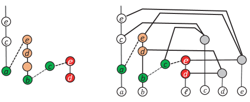
Figure 3: The string $Q=ecaedbced$ (left) and the tree-child network $N(Q,\ell)$ (right), which are derived from the network in Example 1. The dashed lines are used to connect the substrings/paths obtained from different LTSs. The non-labeled orange node had $\ell$ as its label in the original network and was removed to compute $Q$. The network edges are drawn downwards and from left to right and the root is not drawn.

5 NP-hardness of the SCS problem for permutation strings

SCS is already known to be NP-hard when all input strings consist of 2 distinct characters [30]. Let us denote this variant 2-SCS (we further need the trivial constraint that no character appears in every input string). We use this fact to obtain the following NP-hardness result.

Theorem 3

The SCS problem is NP-hard even for permutation strings.

Proof. Consider an instance $\mathcal{S}$ of 2-SCS with $m$ length-2 strings over a size-$n$ alphabet $X=\{x_{1},\ldots,x_{n}\}$, and an integer $k$. Let $N=n+k+1$, and create a size-$N$ set $Y=\{y_{1},\ldots,y_{N}\}$ of separators. In the context of strings, we also write $X$ and $Y$ for the strings $x_{1}\ldots x_{n}$ and $y_{1}\ldots y_{N}$, respectively. For any string $ab\in\mathcal{S}$ (with $a,b\in X$ and $a\neq b$), we write $X_{-ab}$ for the subsequence of $x_{1}x_{2}\ldots x_{n}$ obtained by removing $a$ and $b$, and $S_{ab}=ab\cdot Y\cdot X_{-ab}$. Note that each $S_{ab}$ is a permutation string on $X\cup Y$. Let us write $\mathcal{S}^{\prime}=\{S_{ab},ab\in\mathcal{S}\}$ and $k^{\prime}=k+N+n$. We now prove the following equivalence that completes the reduction.

Strings in $\mathcal{S}$ have a common supersequence $T$ of size $k$

$\Leftrightarrow$ Strings in $\mathcal{S}^{\prime}$ have a common supersequence $T^{\prime}$ of size $k^{\prime}$

$\Rightarrow$ Build $T^{\prime}=T\cdot Y\cdot X$. $T^{\prime}$ is a length-$k^{\prime}$ string, and it is a supersequence of any $S_{ab}$ for $ab\in S^{\prime}$ (since $T$ is a supersequence of $ab$ and $X$ is a supersequence of $X_{-ab}$).

$\Leftarrow$ Pick such a string $T^{\prime}$. It contains at least one occurrence of $Y$ as a subsequence. Let $P,R$ be the matching prefix and suffix of $T^{\prime}$ (i.e. $T^{\prime}=P\cdot R$) such that $R$ is the smallest suffix containing $Y$ as a subsequence. Let $T$ be the subsequence of $P$ obtained by removing all separator characters. We have $|P|\leq k^{\prime}-N=k+n<N$, so $P$ may not contain an entire copy of $Y$. Hence, for any $S_{ab}=ab\cdot Y\cdot X_{-ab}\in\mathcal{S}^{\prime}$, we have that $ab$ is a subsequence of $P$ and $X_{-ab}$ is a subsequence of $R$. Overall, $P$, and also $T$, are common supersequence of all $ab\in\mathcal{S}$, and $R$ is a common supersequence of all $X_{-ab}$. In order to bound their sizes, note that $R$ contains each character of $X$ and $Y$ at least once, so $|R|\geq N+n$. Hence, $T$ has size at most $k^{\prime}-N-n=k$, and is a common supersequence of $\mathcal{S}$. This concludes the proof.

Taken together, Theorem 2 and Theorem 3 imply the following theorem.

Theorem 4

The TCN problem is NP-hard even for line trees.

Open problem 1. Does the TCN problem remain NP-hard for two line trees?

The TCN problem for three line trees was studied by Van Iersel et al. in [28].

6 Tree-child networks that display all the line trees

Theorem 5

The parsimonious tree-child networks that display all the line trees on the taxon set $X$ are identical to that that display all the binary trees.

Proof. Let $\pi:\pi_{1}<\pi_{2}<\cdots<\pi_{n}$ be an arbitary ordering on $X$. Set $X_{i}=\{\pi_{i},\pi_{i+1},\cdots,\pi_{n}\}$. Clearly, $X=X_{1}$. We also use $X_{i}^{k}$ to denote the set of all the strings of length $k$ in which each character appears no more than once, where $k\geq 1$. Let $S_{i}$ be the set of the LTSs of $\pi_{i}$ obtained in all the line trees. For each length-($n-1$) string $s=a_{1}a_{2}\cdots a_{n-1}$ on $X_{2}$, we obtain the line $T(s,\pi_{1})$. Since $\pi_{1}$ is one of the deepest leaf, we conclude that $s$ is the LTS of $\pi$ in $T(s,\pi_{1})$. This implies that $X_{2}^{n-1}\subseteq S_{1}$. Since the LTS of $\pi_{1}$ in any line tree is a string in which each character of $X_{2}$ appears at most once,

$$S_{1}\subseteq X_{2}\cup X_{2}^{2}\cup\cdots\cup X_{2}^{n-1}$$ (5)

Similarly, we can prove that, for each $k\leq n-1$,

$$X_{k+1}^{n-k}\subseteq S_{k}\subseteq X_{k+1}\cup X_{k+1}^{2}\cup\cdots\cup X_{k+1}^{n-k}.$$ (6)

Taken together, Eqn. 5 and 6 implies that for each $k$,

$$|{\rm SCS}(S_{k})|=|{\rm SCS}(X_{k+1}^{n-k})|$$ (7)

In the case for all the trees, Eqn. (5) remains for all $k$. Similarly, Eq. (6 ) is also true. This implies that for any ordering on $A$, the LTSs of any specific taxon in all the lines and in all binary trees have the same SCS. Therefore, the parsimonious trees for all line trees are identical to that for all binary trees. This concludes the proof.

Lemma 1

Let $A$ be a size-$n$ alphabet and let $A_{p}$ denote the set of all permutation strings on $A$. Then,

$$|\mbox{\rm SCS}(A_{p})|=\left\{\begin{array}[]{cc}1,&\mbox{if }n=1;\\ 3,&\mbox{if }n=2;\\ n^{2}-2n+4,&\mbox{ if }3\leq n\leq 7;\end{array}\right.$$

$$n(n+1)/2\leq|\mbox{\rm SCS}(A_{p})|\leq n^{2}-2n+4-\lfloor(n-7)/3\rfloor,\mbox{ if }n\geq 8.$$

Proof. The results for $n\leq 7$ can be verified using computing. For example, the string $1213121$ is a SCS of all the permutation strings on $\{1,2,3\}$. The string $123413214321$ a SCS of all the permutation strings on $\{1,2,3,4\}$. The length-19 string $1234512341523142351$ is a SCS of all the permutation strings on $\{1,2,3,4,5\}$.

For $n\geq 8$, the lower bound was given by Kleitman and Kwiatkowski [31] and the upper bound was proved by Radomirović [32].

Theorem 6

Let $P$ be a parsimonious tree-child network that display all the binary trees on the taxon set $X$. Then, $(n-2)(n-1)(n+3)/6\leq{\rm HN}(P)\leq(n^{3}-5n^{2}+21n-53)/3$, where $n=|X|\geq 8$.

Proof. Let $f(x)=\lfloor(x-7)/3\rfloor$. By Lemma 1, $|{\rm SCS}(S_{k})|=|{\rm SCS}(X_{k+1}^{n-k})|\leq(n-k)^{2}-2(n-k)+4-f(n-k)$ for each $1\leq k\leq n-8$, $|{\rm SCS}(S_{k})|=(n-k)^{2}-2(n-k)+4$ for $n-7\leq k\leq n-3$, $|{\rm SCS}(S_{n-2})|=3$ and $|{\rm SCS}(S_{n-1})|=1$. Therefore, the HN of the tree-child network $Q_{\pi}$ constructed using Tree-Child Network Construction from ${\rm SCS}(S_{k})$ ($1\leq k\leq n-1$) is:

$${\rm HN}(Q_{\pi}) \leq 4+\sum^{n-3}_{k=n-7}[(n-k)^{2}-2(n-k)+4]$$

$$+\sum^{n-8}_{k=1}[(n-k)^{2}-2(n-k)+4-f(n-k)]-(n-1)$$

$$= 5-n+\sum^{n-1}_{j=3}(j^{2}-2j+4)-\sum^{n-1}_{j=8}f(j)$$

$$= 3(n-2)+n(n-1)(2n-7)/6-\sum^{n-1}_{j=8}\lfloor(j-7)/3\rfloor$$

If $n=3k+2,3k$, $k\geq 3$, the last sum is $(n-8)(n-9)/6$. If $n=3k+1,k\geq 3$, the last sum term is $(n-7)(n-10)/6$. Therefore, for $n\geq 8$,

$${\rm HN}(Q_{\pi})\leq(n^{3}-5n^{2}+21n-53)/3.$$

According to Lemma 1, $|{\rm SCS}(S_{k})|=|{\rm SCS}(X_{k+1}^{n-k})|\geq(n-k)(n-k+1)/2$ for $1\leq k\leq n-1$. The lower bound on ${\rm HN}(Q_{\pi})$ is obtained as:

$${\rm HN}(Q_{\pi}) = \sum^{n-1}_{k=1}|{\rm SCS}(S_{k})|-(n-1)$$

$$\geq \sum^{n-1}_{k=1}(n-k)(n-k+1)/2-(n-1)$$

$$= (n-2)(n-1)(n+3)/6.$$

This concludes the proof.

Example 2. For $n\leq 5$, a parsimonious tree-child network for all the 15 binary trees on $\{a,b,c,d\}$ is given in Figure 4.

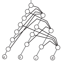
Figure 4: A parsimonious tree-child network with $8$ reticulate nodes that displays all 15 binary trees on taxa $a,b,c,d$. The straight edges are oriented downwards and other edges are oriented from left to right.

7 Conclusions

In this work, we have made two contributions to the study of tree-child networks. Firstly, the tree-child network inference problem remains NP-hard, further fortifying the NP-hardness result originally presented in [26]. To prove the NP-hardness, we prove that the shortest common supersequence problem is also NP-hard, which holds intrinsic interest for the broader scientific community.

Secondly, we have proved that the HN of the so-called ”universal tree-child network” on $n$ taxa is $\Theta(n^{3})$, illuminating the expressive power of tree-child networks.

References

- [1] J. P. Gogarten, J. P. Townsend, Horizontal gene transfer, genome innovation and evolution, Nature Reviews Microbiol. 3 (9) (2005) 679–687.
- [2] E. V. Koonin, K. S. Makarova, L. Aravind, Horizontal gene transfer in prokaryotes: quantification and classification, Annual Rev. Microbiol. 55 (1) (2001) 709–742.
- [3] T. Marcussen, S. R. Sandve, L. Heier, M. Spannagl, M. Pfeifer, The International Wheat Genome Sequencing Consortium, K. S. Jakobsen, B. B. Wulff, B. Steuernagel, K. F. Mayer, O.-A. Olsen, Ancient hybridizations among the ancestral genomes of bread wheat, Science 345 (6194) (2014) 1250092–1250092. doi:10.1126/science.1250092.
- [4] M. C. Fontaine, J. B. Pease, A. Steele, et al., Extensive introgression in a malaria vector species complex revealed by phylogenomics, Science 347 (6217) (2015) 1258524–1258524. doi:0.1126/science.1258524.
- [5] S. Koblmüller, N. Duftner, K. M. Sefc, M. Aibara, M. Stipacek, M. Blanc, B. Egger, C. Sturmbauer, Reticulate phylogeny of gastropod-shell-breeding cichlids from lake tanganyika–the result of repeated introgressive hybridization, BMC Evol. Biol. 7 (1) (2007) 1–13.
- [6] D. Gusfield, ReCombinatorics: the algorithmics of ancestral recombination graphs and explicit phylogenetic networks, MIT press, 2014.
- [7] D. H. Huson, R. Rupp, C. Scornavacca, Phylogenetic networks: concepts, algorithms and applications, Cambridge University Press, 2010.
- [8] M. Steel, Phylogeny: discrete and random processes in evolution, SIAM, 2016.
- [9] R. L. Elworth, H. A. Ogilvie, J. Zhu, L. Nakhleh, Advances in computational methods for phylogenetic networks in the presence of hybridization, in: Bioinformatics and Phylogenetics, Springer, 2019, pp. 317–360.
- [10] L. Zhang, Clusters, trees, and phylogenetic network classes, in: Bioinformatics and Phylogenetics: Seminal Contributions of Bernard Moret, Springer, 2019.
- [11] S. Lutteropp, C. Scornavacca, A. M. Kozlov, B. Morel, A. Stamatakis, Netrax: accurate and fast maximum likelihood phylogenetic network inference, Bioinformatics 38 (15) (2022) 3725–3733.
- [12] C. Solís-Lemus, C. Ané, Inferring phylogenetic networks with maximum pseudolikelihood under incomplete lineage sorting, PLoS genetics 12 (3) (2016) e1005896.
- [13] C. Zhang, H. A. Ogilvie, A. J. Drummond, T. Stadler, Bayesian inference of species networks from multilocus sequence data, Molecular biology and evolution 35 (2) (2018) 504–517.
- [14] J. Pickrell, J. Pritchard, Inference of population splits and mixtures from genome-wide allele frequency data, Nat Prec (2012). doi:10.1038/npre.2012.6956.1.
- [15] L. van Iersel, R. Janssen, M. Jones, Y. Murakami, N. Zeh, A practical fixed-parameter algorithm for constructing tree-child networks from multiple binary trees, Algorithmica 84 (4) (2022) 917–960.
- [16] L. Wang, K. Zhang, L. Zhang, Perfect phylogenetic networks with recombination, Journal of Computational Biology 8 (1) (2001) 69–78.
- [17] D. H. Huson, R. Rupp, V. Berry, P. Gambette, C. Paul, Computing galled networks from real data, Bioinformatics 25 (12) (2009) i85–i93.
- [18] G. Cardona, M. Llabrés, F. Rosselló, G. Valiente, Metrics for phylogenetic networks II: Nodal and triplets metrics, IEEE/ACM-TCBB 6 (3) (2009) 454–469. doi:10.1109/TCBB.2008.127.
- [19] G. Cardona, L. Zhang, Counting and enumerating tree-child networks and their subclasses, Journal of Computer and System Sciences 114 (2020) 84–104.
- [20] L. Zhang, Generating normal networks via leaf insertion and nearest neighbor interchange, BMC Bioinform. 20 (20) (2019) 1–9.
- [21] B. Albrecht, C. Scornavacca, A. Cenci, D. H. Huson, Fast computation of minimum hybridization networks, Bioinformatics 28 (2) (2012) 191–197.
- [22] S. Mirzaei, Y. Wu, Fast construction of near parsimonious hybridization networks for multiple phylogenetic trees, IEEE/ACM Trans. Comput. Biol. Bioinform. 13 (3) (2015) 565–570.
- [23] Y. Wu, Close lower and upper bounds for the minimum reticulate network of multiple phylogenetic trees, Bioinformatics 26 (12) (2010) i140–i148.
- [24] K. Yamada, Z.-Z. Chen, L. Wang, Improved practical algorithms for rooted subtree prune and regraft (rSPR) distance and hybridization number, J. Comput. Biol. 27 (9) (2020) 1422–1432.
- [25] M. Bordewich, C. Semple, Computing the minimum number of hybridization events for a consistent evolutionary history, Discrete Applied. Math. 155 (8) (2007) 914–928.
- [26] S. Linz, C. Semple, Attaching leaves and picking cherries to characterise the hybridisation number for a set of phylogenies, Adv. Applied Math. 105 (2019) 102–129.
- [27] L. Zhang, N. Abhari, C. Colijn, Y. Wu, A fast and scalable method for inferring phylogenetic networks from trees by aligning lineage taxon strings, Genome Research 33 (2023) gr–277669.
- [28] L. van Iersel, M. Jones, M. Weller, When three trees go to war, hal.science (2023).
- [29] M. R. Garey, D. S. Johnson, Computers and intractability, Freeman San Francisco, 1979.
- [30] V. Timkovskii, Complexity of common subsequence and supersequence problems and related problems, Cybernetics 25 (1989) 565–580.
- [31] D. J. Kleitman, D. J. Kwiatkowski, A lower bound on the length of a sequence containing all permutations as subsequences, Journal of Combinatorial Theory, Series A 21 (2) (1976) 129–136.
- [32] S. Radomirović, A construction of short sequences containing all permutations of a set as subsequences, Electronic Journal of Combinatorics 19 (4) (2012) Paper 31.