Influence of Charge on Anisotropic Class-one Solution in Non-minimally Coupled Gravity

Abstract

This paper studies charged star models associated with anisotropic matter distribution in $f(\mathcal{R},\mathcal{T},\mathcal{Q})$ theory, where $\mathcal{Q}=\mathcal{R}_{\phi\psi}\mathcal{T}^{\phi\psi}$. For this purpose, we take a linear model of this gravity as $\mathcal{R}+\zeta\mathcal{Q}$, where $\zeta$ represents a coupling constant. We consider a self-gravitating spherical geometry in the presence of electromagnetic field and generate solution to the modified field equations by using the “embedding class-one” condition and $\mathbb{MIT}$ bag model equation of state. The observational data (masses and radii) of four different stellar models like 4U 1820-30, SAX J 1808.4-3658, SMC X-4 and Her X-I is employed to analyze the effects of charge on their physical properties. Finally, the effect of the coupling constant is checked on the viability, hydrostatic equilibrium condition and stability of the resulting solution. We conclude that the considered models show viable and stable behavior for all the considered values of charge and $\zeta$.

Keywords: $f(\mathcal{R},\mathcal{T},\mathcal{R}_{\phi\psi}\mathcal{T}^{\phi\psi})$ gravity; Stability; Self-gravitating systems; Compact objects.
PACS: 04.50.Kd; 04.40.Dg; 04.40.-b.

1 Introduction

General Relativity ($\mathbb{GR}$) is viewed as the best gravitational theory to tackle various challenges, yet it is inadequately enough to explain the rapid expansion of our cosmos properly. As a result, multiple extensions to $\mathbb{GR}$ have been proposed to deal with mystifying problems such as the dark matter and cosmic expeditious expansion etc. Various cosmologists pointed out that this expansion is caused by the presence of a large amount of an obscure force, named as dark energy which works as anti-gravity and helps stars as well as galaxies to move away from each other. The simplest extension to $\mathbb{GR}$ was obtained by putting the generic function of the Ricci scalar $\mathcal{R}$ in geometric part of the Einstein-Hilbert action, named as $f(\mathcal{R})$ theory [1]. There is a large body of literature [2]-[5] to explore the viability and stability of celestial structures in this theory.

Bertolami et al [6] introduced the concept of matter-geometry coupling in $f(\mathcal{R})$ scenario by coupling the effects of $\mathcal{R}$ in the matter Lagrangian to study self-gravitating objects. Such couplings have prompted many researchers and hence several modifications of $\mathbb{GR}$ (based on the idea of coupling) have been suggested. The first matter-geometry coupling was proposed by Harko et al [7], named as $f(\mathcal{R},\mathcal{T})$ gravity, in which $\mathcal{T}$ serves as trace of the energy-momentum tensor $(\mathbb{EMT})$. The incorporation of $\mathcal{T}$ in modified functionals produces non-null divergence of the corresponding $\mathbb{EMT}$ as opposed to $\mathbb{GR}$ and $f(\mathcal{R})$ theories. This coupling gravity offers several remarkable astrophysical results [8]-[11].

Haghani et al [12] suggested much complicated theory whose functional depends on $\mathcal{R},~{}\mathcal{T}$ and $\mathcal{Q}$, where $\mathcal{Q}\equiv\mathcal{R}_{\phi\psi}\mathcal{T}^{\phi\psi}$. They studied three different models of this theory to analyze their physical viability. The insertion of $\mathcal{R}_{\phi\psi}\mathcal{T}^{\phi\psi}$ makes this theory more effective than other modified theories such as $f(\mathcal{R},\mathbb{L}_{m})$ and $f(\mathcal{R},\mathcal{T})$. The reason is that it entails strong non-minimal interaction between geometry and matter distribution in a self-gravitating object even for the scenarios when $f(\mathcal{R},\mathcal{T})$ fails. For instance, for the case in which a compact interior has trace-free $\mathbb{EMT}$, (i.e., $\mathcal{T}=0$), the particles can entail such strong coupling. This theory provides better understanding of inflationary era of our cosmos as well as rotation curves of galactic structures. Sharif and Zubair [13] adopted matter Lagrangian as $\mathbb{L}_{m}=\mu,~{}-P$ to study thermodynamical laws corresponding to two models $\mathcal{R}+\zeta\mathcal{Q}$ as well as $\mathcal{R}(1+\zeta\mathcal{Q})$ and determined viability constraints for them. The same authors [14] checked the validity of energy bounds analogous to the above models and concluded that only positive values of $\zeta$ fulfill weak energy conditions.

Odintsov and Sáez-Gómez [15] demonstrated certain cosmological solutions and confirmed that $f(\mathcal{R},\mathcal{T},\mathcal{Q})$ gravity supports the $\Lambda$CDM model. Baffou et al [16] obtained numerical solutions of Friedmann equations and perturbation functions with respect to two peculiar modified models and explored their stability. Sharif and Waseem [17, 18] determined the solutions and their stability for isotropic as well anisotropic configurations and concluded that $\mathbb{L}_{m}=P_{r}$ results in more stable structures for the later case. Yousaf et al [19]-[24] employed the idea of orthogonal splitting of the curvature tensor in this gravity and calculated some scalars in the absence and presence of charge which help to understand the structural evolution of self-gravitating bodies. Recently, we have obtained physically acceptable solutions in this scenario through multiple approaches [25]-[29]. The complexity factor and two different evolutionary modes have also been discussed for a self-gravitating object [30, 31].

Numerous investigations have been conducted in the context of $\mathbb{GR}$ and its extended theories to examine how charge influences the structural changes in celestial objects. Das et al. [32] used Riessner-Nordström metric as an exterior geometry and calculated the solution of the equations coupled with charge at the hypersurface. Sunzu et al [33] studied several strange stars owning charged matter configuration in their interiors with the help of mass-radius relation. Various authors [34]-[36] observed that presence of charge inside physical systems usually make them more stable in a wide range.

The state variables for isotropic or anisotropic quark bodies are usually represented by energy density and pressure, that can be interlinked through different constraints, one of them is the $\mathbb{MIT}$ bag model equation of state ($\mathbb{E}$o$\mathbb{S}$) [32]. It is well-known that compactness of strange structures like RXJ 185635-3754, PSR 0943+10, Her X-1, 4U 1820-30, SAX J 1808.4-3658 and 4U 1728-34, etc. can be efficiently described by $\mathbb{MIT}$ $\mathbb{E}$o$\mathbb{S}$, whereas an $\mathbb{E}$o$\mathbb{S}$ for neutron star fails in this context [37]. In general, a vacuum comprises of two states, namely false and true whose discrepancy can be calculated through the bag constant ($\mathfrak{B}$). This model has extensively been used by several researchers [38]-[40] to analyze the internal composition of various quark bodies. Demorest et al [41] discussed a particular strange star (namely, PSR J1614-2230) and found that class of such massive objects can only be supported by $\mathbb{MIT}$ bag model. Rahaman et al [42] employed this model along with interpolating technique to explore the mass and some other physical aspects of compact structures.

The solution to the field equations in any gravitational theory can be formulated by virtue of multiple techniques, such as the consideration of a particular $\mathbb{E}$o$\mathbb{S}$ or the solution of metric potentials etc. A useful technique in this regard is the embedding class-one condition which points out that an $n$-dimensional space can always be embedded into a space of one more dimension, i.e., $n+1$. Bhar et al [43] used an acceptable metric potential to determine physically viable anisotropic star models through this condition. Maurya et al [44, 45] employed this condition to calculate the solutions corresponding to relativistic stars and also analyzed the effects of anisotropy on these structures. Singh et al [46] formed non-singular solution for spherically symmetric spacetime in terms of new metric function by using this technique. The decoupled solutions for self-gravitating anisotropic systems have been determined through class-one condition [47, 48]. The same condition has also been employed to modified theories. Singh et al [49] used the embedding approach to study the physical features of different compact stars in the context of $f(\mathcal{R},\mathcal{T})$ theory. Rahaman et al [50] also discussed celestial structures through an embedding approach in the same scenario and claimed that this modified theory better explains such massive bodies. Various authors formulated multiple acceptable class-one solutions in various backgrounds such as $f(\mathcal{R}),~{}f(\mathcal{G}),~{}f(\mathcal{R},\mathcal{T})$ and $f(\mathcal{G},\mathcal{T})$ theories [51]-[60]. Sharif and his collaborators [61]-[63] extended this work in $f(\mathcal{G})$ and Brans-Dicke scenarios, and obtained viable as well as stable solutions.

In this paper, we study charged star models with anisotropic matter distribution in the framework of $f(\mathcal{R},\mathcal{T},\mathcal{Q})$ theory. The paper has the following format. Next section is devoted to the basic description of modified theory and construction of the field equations corresponding to a model $\mathcal{R}+\zeta\mathcal{Q}$. We assume $\mathbb{MIT}$ bag model $\mathbb{E}$o$\mathbb{S}$ and utilize embedding condition to find radial metric potential from known temporal component. The boundary conditions are given in section 3. Section 4 explores the effects of electromagnetic field on several physical characteristics of compact objects through graphical analysis. Finally, we summarize all the results in section 5.

2 The $f(\mathcal{R},\mathcal{T},\mathcal{Q})$ Gravity

The action for this theory is obtained by inserting $f(\mathcal{R},\mathcal{T},\mathcal{Q})$ in place of $\mathcal{R}$ in the Einstein-Hilbert action (with $\kappa=8\pi$) as [15]

$$\mathbb{I}_{f(\mathcal{R},\mathcal{T},\mathcal{Q})}=\int\sqrt{-g}\left\{\frac{f(\mathcal{R},\mathcal{T},\mathcal{Q})}{16\pi}+\mathbb{L}_{m}+\mathbb{L}_{\mathcal{E}}\right\}d^{4}x,$$ (1)

where $\mathbb{L}_{m}$ and $\mathbb{L}_{\mathcal{E}}$ symbolize the Lagrangian densities of matter configuration and electromagnetic field, respectively. The corresponding field equations are

$$\mathcal{G}_{\phi\psi}=\mathcal{T}_{\phi\psi}^{(\mathrm{EFF})}=8\pi\bigg{\{}\frac{1}{f_{\mathcal{R}}-\mathbb{L}_{m}f_{\mathcal{Q}}}\left(\mathcal{T}_{\phi\psi}+\mathcal{E}_{\phi\psi}\right)+\mathcal{T}_{\phi\psi}^{(\mathcal{C})}\bigg{\}},$$ (2)

where $\mathcal{G}_{\phi\psi}$ is the Einstein tensor, $\mathcal{T}_{\phi\psi}^{(\mathrm{EFF})}$ can be termed as the $\mathbb{EMT}$ in extended gravity, $\mathcal{T}_{\phi\psi}$ is the matter energy-momentum tensor and $\mathcal{E}_{\phi\psi}$ is the electromagnetic tensor. The modified sector of this theory becomes

$$\mathcal{T}_{\phi\psi}^{(\mathcal{C})} = -\frac{1}{8\pi\bigg{(}\mathbb{L}_{m}f_{\mathcal{Q}}-f_{\mathcal{R}}\bigg{)}}\left[\left(f_{\mathcal{T}}+\frac{1}{2}\mathcal{R}f_{\mathcal{Q}}\right)\mathcal{T}_{\phi\psi}+\left\{\frac{\mathcal{R}}{2}(\frac{f}{\mathcal{R}}-f_{\mathcal{R}})-\mathbb{L}_{m}f_{\mathcal{T}}\right.\right.$$ (3)

$$- \left.\frac{1}{2}\nabla_{\sigma}\nabla_{\omega}(f_{\mathcal{Q}}\mathcal{T}^{\sigma\omega})\right\}g_{\phi\psi}-\frac{1}{2}\Box(f_{\mathcal{Q}}\mathcal{T}_{\phi\psi})-(g_{\phi\psi}\Box-\nabla_{\phi}\nabla_{\psi})f_{\mathcal{R}}$$

$$- 2f_{\mathcal{Q}}\mathcal{R}_{\sigma(\phi}\mathcal{T}_{\psi)}^{\sigma}+\nabla_{\sigma}\nabla_{(\phi}[\mathcal{T}_{\psi)}^{\sigma}f_{\mathcal{Q}}]+2(f_{\mathcal{Q}}\mathcal{R}^{\sigma\omega}+\left.f_{\mathcal{T}}g^{\sigma\omega})\frac{\partial^{2}\mathbb{L}_{m}}{\partial g^{\phi\psi}\partial g^{\sigma\omega}}\right].$$

Here, $f_{\mathcal{R}},~{}f_{\mathcal{T}}$ and $f_{\mathcal{Q}}$ are the partial derivatives of $f$ with respect to its arguments. Also, $\Box\equiv\frac{1}{\sqrt{-g}}\partial_{\phi}\big{(}\sqrt{-g}g^{\phi\psi}\partial_{\psi}\big{)}$ and $\nabla_{\omega}$ indicate D’Alambert operator and covariant derivative, respectively. We take suitable choice of matter Lagrangian as $\mathbb{L}_{m}=-\frac{1}{4}\mathcal{A}_{\phi\psi}\mathcal{A}^{\phi\psi}$ which leads to $\frac{\partial^{2}\mathbb{L}_{m}}{\partial g^{\phi\psi}\partial g^{\sigma\omega}}=-\frac{1}{2}\mathcal{A}_{\phi\sigma}\mathcal{A}_{\psi\omega}$ [12]. Here, $\mathcal{A}_{\phi\psi}=\omega_{\psi;\phi}-\omega_{\phi;\psi}$ serves as the Maxwell field tensor and $\omega_{\psi}=\omega(r)\delta^{\psi}_{0}$ is termed as the four potential. The violation of the equivalence principle is obvious in this theory due to the arbitrary coupling between matter and geometry which results in the disappearance of covariant divergence of $\mathbb{EMT}$ (3) (i.e., $\nabla_{\phi}\mathcal{T}^{\phi\psi}\neq 0$). Consequently, an additional force is produced in the gravitational structure which causes non-geodesic motion of test particles. Thus we have

$$\nabla^{\phi}\mathcal{T}_{\phi\psi} =\frac{2}{2f_{\mathcal{T}}+\mathcal{R}f_{\mathcal{Q}}+16\pi}\bigg{[}\nabla_{\phi}\big{(}f_{\mathcal{Q}}\mathcal{R}^{\sigma\phi}\mathcal{T}_{\sigma\psi}\big{)}-\mathcal{G}_{\phi\psi}\nabla^{\phi}\big{(}f_{\mathcal{Q}}\mathbb{L}_{m}\big{)}$$

$$-\frac{1}{2}\nabla_{\psi}\mathcal{T}^{\sigma\omega}\big{(}f_{\mathcal{T}}g_{\sigma\omega}+f_{\mathcal{Q}}\mathcal{R}_{\sigma\omega}\big{)}+\nabla_{\psi}\big{(}\mathbb{L}_{m}f_{\mathcal{T}}\big{)}-8\pi\nabla^{\phi}\mathcal{E}_{\phi\psi}\bigg{]}.$$ (4)

In the structural development of celestial bodies, anisotropy is supposed as a basic entity which appears when there is a difference between radial and tangential pressures. In our cosmos, many stars are likely to be interlinked with anisotropic fluid, thus this factor becomes highly significant in the study of stellar models and their evolution. The anisotropic $\mathbb{EMT}$ is

$$\mathcal{T}_{\phi\psi}=(\mu+P_{\bot})\mathcal{K}_{\phi}\mathcal{K}_{\psi}+P_{\bot}g_{\phi\psi}+\left(P_{r}-P_{\bot}\right)\mathcal{W}_{\phi}\mathcal{W}_{\psi},$$ (5)

where the energy density, radial as well as tangential pressure, four-vector and four-velocity are given by $\mu,~{}P_{r},~{}P_{\bot},~{}\mathcal{W}_{\phi}$ and $\mathcal{K}_{\phi}$, respectively. The trace of the field equations provides

$$3\nabla^{\omega}\nabla_{\omega}f_{\mathcal{R}}-\mathcal{R}\left(\frac{\mathcal{T}}{2}f_{\mathcal{Q}}-f_{\mathcal{R}}\right)-\mathcal{T}(8\pi+f_{\mathcal{T}})+\frac{1}{2}\nabla^{\omega}\nabla_{\omega}(f_{\mathcal{Q}}\mathcal{T})$$

$$+\nabla_{\phi}\nabla_{\omega}(f_{\mathcal{Q}}\mathcal{T}^{\phi\omega})-2f+(\mathcal{R}f_{\mathcal{Q}}+4f_{\mathcal{T}})\mathbb{L}_{m}+2\mathcal{R}_{\phi\omega}\mathcal{T}^{\phi\omega}f_{\mathcal{Q}}$$

$$-2g^{\psi\xi}\frac{\partial^{2}\mathbb{L}_{m}}{\partial g^{\psi\xi}\partial g^{\phi\omega}}\left(f_{\mathcal{T}}g^{\phi\omega}+f_{\mathcal{Q}}R^{\phi\omega}\right)=0.$$

For $f_{\mathcal{Q}}=0$, this yields $f(\mathcal{R},\mathcal{T})$ theory, which can further be reduced to $f(\mathcal{R})$ gravity when $f_{\mathcal{T}}=0$. The electromagnetic $\mathbb{EMT}$ is defined as

$$\mathcal{E}_{\phi\psi}=\frac{1}{4\pi}\left[\frac{1}{4}g_{\phi\psi}\mathcal{A}^{\sigma\omega}\mathcal{A}_{\sigma\omega}-\mathcal{A}^{\omega}_{\phi}\mathcal{A}_{\omega\psi}\right],$$

and Maxwell equations are

$$\mathcal{A}^{\phi\psi}_{;\psi}=4\pi\mathcal{J}^{\phi},\quad\mathcal{A}_{[\phi\psi;\sigma]}=0,$$

where $\mathcal{J}^{\phi}=\varpi\mathcal{K}^{\phi}$, $\mathcal{J}^{\phi}$ and $\varpi$ are the current and charge densities, respectively. To examine the interior compact stars, we take self-gravitating spherical spacetime as

$$ds^{2}=-e^{\rho}dt^{2}+e^{\alpha}dr^{2}+r^{2}d\theta^{2}+r^{2}\sin^{2}\theta d\varphi^{2},$$ (6)

where $\rho=\rho(r)$ and $\alpha=\alpha(r)$. The Maxwell equations

$$\omega^{\prime\prime}+\frac{1}{2r}\big{[}4-r(\rho^{\prime}+\alpha^{\prime})\big{]}\omega^{\prime}=4\pi\varpi e^{\frac{\rho}{2}+\alpha},$$ (7)

lead to

$$\omega^{\prime}=\frac{s}{r^{2}}e^{\frac{\rho+\alpha}{2}},$$ (8)

where $s$ shows the presence of charge inside the geometry (6) and ${}^{\prime}=\frac{\partial}{\partial r}$. In this context, the matter Lagrangian turns out to be $\mathbb{L}_{m}=\frac{s^{2}}{2r^{4}}$. Also, the four-vector and four-velocity in comoving framework are

$$\mathcal{W}^{\phi}=\delta^{\phi}_{1}e^{\frac{-\alpha}{2}},\quad\mathcal{K}^{\phi}=\delta^{\phi}_{0}e^{\frac{-\rho}{2}},$$ (9)

satisfying $\mathcal{K}^{\phi}\mathcal{K}_{\phi}=-1$ and $\mathcal{W}^{\phi}\mathcal{K}_{\phi}=0$.

We consider a linear model as [12]

$$f(\mathcal{R},\mathcal{T},\mathcal{R}_{\phi\psi}\mathcal{T}^{\phi\psi})=f_{1}(\mathcal{R})+f_{2}(\mathcal{R}_{\phi\psi}\mathcal{T}^{\phi\psi})=\mathcal{R}+\zeta\mathcal{R}_{\phi\psi}\mathcal{T}^{\phi\psi},$$ (10)

where $\zeta$ is an arbitrary coupling constant. The nature of the corresponding solution is found to be oscillatory (representing alternating collapsing and expanding phases) for the case when $\zeta>0$. On the other hand, $\zeta<0$ yields the cosmic scale factor having a hyperbolic cosine-type dependence. The stability of this model has been analyzed for isotropic/anisotropic configurations through different schemes leading to some acceptable values of $\zeta$ [13, 14, 17]. The factor $\mathcal{Q}$ of this model becomes

$$\mathcal{Q} = e^{-\alpha}\bigg{[}\frac{\mu}{4}\left(2\rho^{\prime\prime}+\rho^{\prime 2}-\rho^{\prime}\alpha^{\prime}+\frac{4\rho^{\prime}}{r}\right)+\frac{P_{r}}{4}\left(\rho^{\prime}\alpha^{\prime}-\rho^{\prime 2}-2\rho^{\prime\prime}-\frac{4\alpha^{\prime}}{r}\right)$$

$$- P_{\bot}\left(\frac{\rho^{\prime}}{r}-\frac{\alpha^{\prime}}{r}-\frac{2e^{\alpha}}{r^{2}}+\frac{2}{r^{2}}\right)\bigg{]}.$$

The corresponding field equations (2) take the form as

$$\mathcal{G}_{\phi\psi} = \frac{\zeta}{1-\frac{\zeta s^{2}}{2r^{4}}}\bigg{[}\left(\frac{8\pi}{\zeta}+\frac{1}{2}\mathcal{R}\right)\mathcal{T}_{\phi\psi}+\frac{8\pi}{\zeta}\mathcal{E}_{\phi\psi}+\frac{1}{2}\left\{\mathcal{Q}-\nabla_{\sigma}\nabla_{\omega}\mathcal{T}^{\sigma\omega}\right\}g_{\phi\psi}$$ (11)

$$- 2\mathcal{R}_{\sigma(\phi}\mathcal{T}_{\psi)}^{\sigma}-\frac{1}{2}\Box\mathcal{T}_{\phi\psi}+\nabla_{\sigma}\nabla_{(\phi}\mathcal{T}_{\psi)}^{\sigma}-\mathcal{R}^{\sigma\omega}\mathcal{A}_{\phi\sigma}\mathcal{A}_{\psi\omega}\bigg{]}.$$

The non-conservation of $\mathbb{EMT}$ (4) becomes

$$\nabla^{\phi}\mathcal{T}_{\phi\psi} =\frac{2\zeta}{\zeta\mathcal{R}+16\pi}\bigg{[}\nabla_{\phi}(\mathcal{R}^{\sigma\phi}\mathcal{T}_{\sigma\psi})-\frac{1}{2}\mathcal{R}_{\sigma\omega}\nabla_{\psi}\mathcal{T}^{\sigma\omega}-\frac{1}{2}\mathcal{T}_{\phi\psi}\nabla^{\phi}\mathcal{R}-8\pi\nabla^{\phi}\mathcal{E}_{\phi\psi}$$

$$-\mathcal{G}_{\phi\psi}\nabla^{\phi}\big{(}\mathbb{L}_{m}\big{)}\bigg{]}.$$ (12)

Equation (11) leads to three non-zero components as

$$8\pi\mu =e^{-\alpha}\bigg{[}\frac{\alpha^{\prime}}{r}+\frac{e^{\alpha}}{r^{2}}-\frac{1}{r^{2}}+\zeta\bigg{\{}\mu\bigg{(}\frac{3\rho^{\prime}\alpha^{\prime}}{8}-\frac{\rho^{\prime 2}}{8}+\frac{\alpha^{\prime}}{r}+\frac{e^{\alpha}}{r^{2}}-\frac{3\rho^{\prime\prime}}{4}-\frac{3\rho^{\prime}}{2r}$$

$$-\frac{1}{r^{2}}\bigg{)}-\mu^{\prime}\bigg{(}\frac{\alpha^{\prime}}{4}-\frac{1}{r}-\rho^{\prime}\bigg{)}+\frac{\mu^{\prime\prime}}{2}+P_{r}\bigg{(}\frac{\rho^{\prime}\alpha^{\prime}}{8}-\frac{\rho^{\prime 2}}{8}-\frac{\rho^{\prime\prime}}{4}+\frac{\alpha^{\prime}}{2r}+\frac{\alpha^{\prime\prime}}{2}$$

$$-\frac{3\alpha^{\prime 2}}{4}\bigg{)}+\frac{5\alpha^{\prime}P^{\prime}_{r}}{4}-\frac{P^{\prime\prime}_{r}}{2}+P_{\bot}\bigg{(}\frac{\alpha^{\prime}}{2r}-\frac{\rho^{\prime}}{2r}+\frac{3e^{\alpha}}{r^{2}}-\frac{1}{r^{2}}\bigg{)}-\frac{P^{\prime}_{\bot}}{r}$$

$$+\frac{s^{2}}{r^{4}}\bigg{(}\frac{\alpha^{\prime}}{2r}-\frac{e^{\alpha}}{2r^{2}}+\frac{1}{2r^{2}}+\frac{\rho^{\prime}\alpha^{\prime}}{8}-\frac{\rho^{\prime 2}}{8}-\frac{\rho^{\prime\prime}}{4}-\frac{e^{\alpha}}{\zeta}\bigg{)}\bigg{\}}\bigg{]},$$ (13)

$$8\pi P_{r} =e^{-\alpha}\bigg{[}\frac{\rho^{\prime}}{r}-\frac{e^{\alpha}}{r^{2}}+\frac{1}{r^{2}}+\zeta\bigg{\{}\mu\bigg{(}\frac{\rho^{\prime}\alpha^{\prime}}{8}+\frac{\rho^{\prime 2}}{8}-\frac{\rho^{\prime\prime}}{4}-\frac{\rho^{\prime}}{2r}\bigg{)}-\frac{\rho^{\prime}\mu^{\prime}}{4}$$

$$-P_{r}\bigg{(}\frac{5\rho^{\prime 2}}{8}-\frac{7\rho^{\prime}\alpha^{\prime}}{8}+\frac{5\rho^{\prime\prime}}{4}-\frac{7\alpha^{\prime}}{2r}+\frac{\rho^{\prime}}{r}-\alpha^{\prime 2}-\frac{e^{\alpha}}{r^{2}}+\frac{1}{r^{2}}\bigg{)}$$

$$+P^{\prime}_{r}\bigg{(}\frac{\rho^{\prime}}{4}+\frac{1}{r}\bigg{)}-P_{\bot}\bigg{(}\frac{\alpha^{\prime}}{2r}-\frac{\rho^{\prime}}{2r}+\frac{3e^{\alpha}}{r^{2}}-\frac{1}{r^{2}}\bigg{)}+\frac{P^{\prime}_{\bot}}{r}$$

$$+\frac{s^{2}}{r^{4}}\bigg{(}\frac{\rho^{\prime}}{2r}+\frac{e^{\alpha}}{2r^{2}}-\frac{1}{2r^{2}}+\frac{\rho^{\prime\prime}}{4}+\frac{\rho^{\prime 2}}{8}-\frac{\rho^{\prime}\alpha^{\prime}}{8}+\frac{e^{\alpha}}{\zeta}\bigg{)}\bigg{\}}\bigg{]},$$ (14)

$$8\pi P_{\bot} =e^{-\alpha}\bigg{[}\frac{1}{2}\bigg{(}\rho^{\prime\prime}+\frac{\rho^{\prime 2}}{2}-\frac{\rho^{\prime}\alpha^{\prime}}{2}-\frac{\alpha^{\prime}}{r}+\frac{\rho^{\prime}}{r}\bigg{)}+\zeta\bigg{\{}\mu\bigg{(}\frac{\rho^{\prime 2}}{8}+\frac{\rho^{\prime}\alpha^{\prime}}{8}-\frac{\rho^{\prime\prime}}{4}-\frac{\rho^{\prime}}{2r}\bigg{)}$$

$$-\frac{\mu^{\prime}\rho^{\prime}}{4}+P_{r}\bigg{(}\frac{\rho^{\prime 2}}{8}+\frac{3\alpha^{\prime 2}}{4}-\frac{\rho^{\prime}\alpha^{\prime}}{8}+\frac{\rho^{\prime\prime}}{4}-\frac{\alpha^{\prime}}{2r}-\frac{\alpha^{\prime\prime}}{2}\bigg{)}-\frac{5\alpha^{\prime}P^{\prime}_{r}}{4}+\frac{P^{\prime\prime}_{r}}{2}$$

$$-P_{\bot}\bigg{(}\frac{\rho^{\prime 2}}{4}-\frac{\rho^{\prime}\alpha^{\prime}}{4}+\frac{\rho^{\prime\prime}}{2}-\frac{\alpha^{\prime}}{r}+\frac{\rho^{\prime}}{r}\bigg{)}-P^{\prime}_{\bot}\bigg{(}\frac{\alpha^{\prime}}{4}-\frac{\rho^{\prime}}{4}-\frac{3}{r}\bigg{)}+\frac{P^{\prime\prime}_{\bot}}{2}$$

$$+\frac{s^{2}}{r^{4}}\bigg{(}\frac{\rho^{\prime}\alpha^{\prime}}{8}-\frac{\rho^{\prime 2}}{8}-\frac{\rho^{\prime\prime}}{4}+\frac{\alpha^{\prime}}{4r}-\frac{\rho^{\prime}}{4r}-\frac{e^{\alpha}}{\zeta}\bigg{)}\bigg{\}}\bigg{]}.$$ (15)

The explicit expressions for the matter variables are given in Eqs.(A1)-(A3). In order to keep the system in hydrostatic equilibrium, we can obtain the corresponding condition from Eq.(12) as

$$\frac{dP_{r}}{dr}+\frac{\rho^{\prime}}{2}\left(\mu+P_{r}\right)-\frac{2}{r}\left(P_{\bot}-P_{r}\right)-\frac{2\zeta e^{-\alpha}}{\zeta\mathcal{R}+16\pi}\bigg{[}\frac{\rho^{\prime}\mu}{8}\bigg{(}\rho^{\prime 2}+2\rho^{\prime\prime}-\rho^{\prime}\alpha^{\prime}+\frac{4\rho^{\prime}}{r}\bigg{)}$$

$$-\frac{\mu^{\prime}}{8}\bigg{(}\rho^{\prime 2}-\rho^{\prime}\alpha^{\prime}+2\rho^{\prime\prime}+\frac{4\rho^{\prime}}{r}\bigg{)}+P_{r}\bigg{(}\frac{5\rho^{\prime 2}\alpha^{\prime}}{8}-\frac{5\rho^{\prime}\alpha^{\prime 2}}{8}-\frac{5\alpha^{\prime 2}}{2r}+\frac{7\rho^{\prime\prime}\alpha^{\prime}}{4}-\frac{\rho^{\prime\prime\prime}}{2}$$

$$-\rho^{\prime}\rho^{\prime\prime}+\frac{\rho^{\prime}\alpha^{\prime\prime}}{2}+\frac{2\alpha^{\prime\prime}}{r}+\frac{\rho^{\prime}\alpha^{\prime}}{r}-\frac{\alpha^{\prime}}{r^{2}}-\frac{\rho^{\prime\prime}}{r}+\frac{\rho^{\prime}}{r^{2}}+\frac{2e^{\alpha}}{r^{3}}-\frac{2}{r^{3}}\bigg{)}+\frac{P^{\prime}_{r}}{8}\bigg{(}\rho^{\prime}\alpha^{\prime}-2\rho^{\prime\prime}$$

$$-\rho^{\prime 2}+\frac{4\alpha^{\prime}}{r}\bigg{)}+\frac{P_{\bot}}{r^{2}}\bigg{(}\alpha^{\prime}-\rho^{\prime}+\frac{2e^{\alpha}}{r}-\frac{2}{r}\bigg{)}-\frac{P^{\prime}_{\bot}}{r}\bigg{(}\frac{\alpha^{\prime}}{2}-\frac{\rho^{\prime}}{2}+\frac{e^{\alpha}}{r}-\frac{1}{r}\bigg{)}$$

$$-\bigg{(}\frac{ss^{\prime}}{r^{4}}-\frac{2s^{2}}{r^{5}}\bigg{)}\left(\frac{\rho^{\prime}}{r}-\frac{e^{\alpha}}{r^{2}}+\frac{1}{r^{2}}+\frac{2e^{\alpha}}{\zeta}\right)\bigg{]}=0.$$ (16)

This represents Tolman-Opphenheimer-Volkoff ($\mathbb{TOV}$) equation in extended framework which helps in analyzing the structure and dynamics of self-gravitating celestial objects. Misner-Sharp [64] provided the mass of a sphere as

$$m(r)=\frac{r}{2}\big{(}1-g^{\phi\psi}r_{,\phi}r_{,\psi}\big{)},$$

which leads to

$$m(r)=\frac{r}{2}\left(1-e^{-\alpha}+\frac{s^{2}}{r^{2}}\right).$$ (17)

The non-linear system (13)-(15) contain six unknowns $\rho,~{}\alpha,~{}\mu,$ $P_{r},~{}P_{\bot}$ and $s$, hence some constraints are required to close the system. We investigate various physical aspects of different quark bodies through a well-known $\mathbb{MIT}$ bag model $\mathbb{E}o\mathbb{S}$ which interrelates the matter variables inside the geometry [32]. This constraint has the form

$$P_{r}=\frac{1}{3}\left(\mu-4\mathfrak{B}\right).$$ (18)

The constant $\mathfrak{B}$ has been determined corresponding to different stars [65, 66] that are used in the analysis of physical attributes of all the considered star models. The solution of the modified field equations (13)-(15) along with $\mathbb{E}o\mathbb{S}$ (18) turns out to be

$$\mu =\bigg{[}8\pi e^{\alpha}+\zeta\bigg{(}\frac{9\rho^{\prime\prime}}{8}-\frac{e^{\alpha}}{r^{2}}+\frac{1}{r^{2}}-\frac{\alpha^{\prime\prime}}{8}-\frac{5\rho^{\prime}\alpha^{\prime}}{8}-\frac{\alpha^{\prime 2}}{16}-\frac{7\alpha^{\prime}}{2r}+\frac{3\rho^{\prime 2}}{16}+\frac{7\rho^{\prime}}{4r}\bigg{)}\bigg{]}^{-1}$$

$$\times\bigg{[}\frac{3}{4}\bigg{(}1+\frac{\zeta s^{2}}{2r^{4}}\bigg{)}\bigg{(}\frac{\alpha^{\prime}}{r}+\frac{\rho^{\prime}}{r}\bigg{)}+\mathfrak{B}\bigg{\{}8\pi e^{\alpha}-\zeta\bigg{(}\frac{4\alpha^{\prime}}{r}-\frac{3\rho^{\prime 2}}{4}-\frac{3\rho^{\prime\prime}}{2}+\rho^{\prime}\alpha^{\prime}$$

$$\frac{\alpha^{\prime\prime}}{2}+\frac{\alpha^{\prime 2}}{4}-\frac{\rho^{\prime}}{r}+\frac{e^{\alpha}}{r^{2}}-\frac{1}{r^{2}}\bigg{)}\bigg{\}}\bigg{]},$$ (19)

$$P_{r} =\bigg{[}8\pi e^{\alpha}+\zeta\bigg{(}\frac{9\rho^{\prime\prime}}{8}-\frac{e^{\alpha}}{r^{2}}+\frac{1}{r^{2}}-\frac{\alpha^{\prime\prime}}{8}-\frac{5\rho^{\prime}\alpha^{\prime}}{8}-\frac{\alpha^{\prime 2}}{16}-\frac{7\alpha^{\prime}}{2r}+\frac{3\rho^{\prime 2}}{16}+\frac{7\rho^{\prime}}{4r}\bigg{)}\bigg{]}^{-1}$$

$$\times\bigg{[}\frac{1}{4}\bigg{(}1+\frac{\zeta s^{2}}{2r^{4}}\bigg{)}\bigg{(}\frac{\alpha^{\prime}}{r}+\frac{\rho^{\prime}}{r}\bigg{)}-\mathfrak{B}\bigg{\{}8\pi e^{\alpha}-\zeta\bigg{(}\frac{\rho^{\prime}\alpha^{\prime}}{2}+\frac{\alpha^{\prime}}{r}-\frac{2\rho^{\prime}}{r}+\frac{e^{\alpha}}{r^{2}}$$

$$-\rho^{\prime\prime}-\frac{1}{r^{2}}\bigg{)}\bigg{\}}\bigg{]},$$ (20)

$$P_{\bot} =\bigg{[}8\pi e^{\alpha}+\zeta\bigg{(}\frac{1}{r^{2}}-\frac{2e^{\alpha}}{r^{2}}+\frac{\rho^{\prime 2}}{4}+\frac{\rho^{\prime\prime}}{2}-\frac{\rho^{\prime}\alpha^{\prime}}{4}+\frac{\rho^{\prime}}{r}-\frac{\alpha^{\prime}}{r}\bigg{)}\bigg{]}^{-1}\bigg{[}\frac{\rho^{\prime}}{2r}-\frac{\alpha^{\prime}}{2r}$$

$$+\frac{\rho^{\prime 2}}{4}-\frac{\rho^{\prime}\alpha^{\prime}}{4}+\frac{\rho^{\prime\prime}}{2}+\zeta\bigg{\{}8\pi e^{\alpha}+\zeta\bigg{(}\frac{9\rho^{\prime\prime}}{8}-\frac{e^{\alpha}}{r^{2}}+\frac{1}{r^{2}}-\frac{\alpha^{\prime\prime}}{8}-\frac{5\rho^{\prime}\alpha^{\prime}}{8}-\frac{\alpha^{\prime 2}}{16}$$

$$-\frac{7\alpha^{\prime}}{2r}+\frac{3\rho^{\prime 2}}{16}+\frac{7\rho^{\prime}}{4r}\bigg{)}\bigg{\}}^{-1}\bigg{\{}\frac{1}{8r}\bigg{(}1+\frac{\zeta s^{2}}{2r^{4}}\bigg{)}\bigg{(}2\rho^{\prime}\alpha^{\prime 2}+\rho^{\prime 3}-\rho^{\prime\prime}\alpha^{\prime}-\rho^{\prime}\rho^{\prime\prime}$$

$$-\alpha^{\prime}\alpha^{\prime\prime}-\rho^{\prime}\alpha^{\prime\prime}+\frac{3\rho^{\prime 2}\alpha^{\prime}}{2}-\frac{3\rho^{\prime 2}}{r}+\frac{3\alpha^{\prime 3}}{2}-\frac{\alpha^{\prime 2}}{r}-\frac{4\rho^{\prime}\alpha^{\prime}}{r}\bigg{)}+2\pi e^{\alpha}\mathfrak{B}\bigg{(}\rho^{\prime}\alpha^{\prime}$$

$$-2\rho^{\prime\prime}+2\alpha^{\prime\prime}-3\alpha^{\prime 2}-\frac{2\rho^{\prime}}{r}+\frac{2\alpha^{\prime}}{r}\bigg{)}+\frac{\zeta\mathfrak{B}}{16}\bigg{(}10\rho^{\prime\prime}\alpha^{\prime\prime}-5\rho^{\prime}\alpha^{\prime}\alpha^{\prime\prime}+11\rho^{\prime}\rho^{\prime\prime}\alpha^{\prime}$$

$$-11\rho^{\prime\prime}\alpha^{\prime 2}-\rho^{\prime 2}\alpha^{\prime\prime}-2\rho^{\prime\prime}\rho^{\prime 2}-10\rho^{\prime\prime 2}-\frac{7\rho^{\prime 2}\alpha^{\prime 2}}{2}+\frac{\rho^{\prime 3}\alpha^{\prime}}{2}-\frac{36\rho^{\prime}\alpha^{\prime 2}}{r}-\frac{8\rho^{\prime 3}}{r}$$

$$+\frac{11\rho^{\prime}\alpha^{\prime 3}}{2}+\frac{16\rho^{\prime 2}\alpha^{\prime}}{r}+\frac{28\rho^{\prime\prime}\alpha^{\prime}}{r}-\frac{8\alpha^{\prime}\alpha^{\prime\prime}}{r}+\frac{12\alpha^{\prime 3}}{r}+\frac{3\rho^{\prime 4}}{2}-\frac{8\rho^{\prime 2}}{r^{2}}-\frac{8\alpha^{\prime\prime}e^{\alpha}}{r^{2}}$$

$$+\frac{8\alpha^{\prime\prime}}{r^{2}}-\frac{20\alpha^{\prime 2}}{r^{2}}-\frac{24\rho^{\prime}\rho^{\prime\prime}}{r}+\frac{52\rho^{\prime}\alpha^{\prime}}{r^{2}}+\frac{10\rho^{\prime}\alpha^{\prime\prime}}{r}-\frac{4e^{\alpha}\rho^{\prime}\alpha^{\prime}}{r^{2}}+\frac{8e^{\alpha}\rho^{\prime\prime}}{r^{2}}-\frac{8\rho^{\prime\prime}}{r^{2}}$$

$$+\frac{12\alpha^{\prime 2}e^{\alpha}}{r^{2}}-\frac{8\rho^{\prime}}{r^{3}}-\frac{8e^{\alpha}\alpha^{\prime}}{r^{3}}+\frac{8\alpha^{\prime}}{r^{3}}+\frac{8e^{\alpha}\rho^{\prime}}{r^{3}}\bigg{)}\bigg{\}}\bigg{]}+\frac{\zeta s^{2}}{4r^{4}e^{\alpha}}\bigg{(}\frac{\rho^{\prime}\alpha^{\prime}}{2}-\frac{\rho^{\prime 2}}{2}-\rho^{\prime\prime}$$

$$+\frac{\alpha^{\prime}}{r}-\frac{\rho^{\prime}}{r}-\frac{4e^{\alpha}}{\zeta}\bigg{)}.$$ (21)

A comprehensive analysis has been done on the study of celestial bodies configured with quark matter through $\mathbb{E}o\mathbb{S}$ (18) in $\mathbb{GR}$ and other modified theories [67, 68]. We find solution to the modified charged field equations by employing this $\mathbb{E}o\mathbb{S}$ and setting values of the coupling constant as $\zeta=\pm 5$.

Eiesland [69] computed the essential and adequate condition for the case of an embedding class-one as

$$\mathcal{R}_{1212}\mathcal{R}_{0303}-\mathcal{R}_{0101}\mathcal{R}_{2323}+\mathcal{R}_{1202}\mathcal{R}_{1303}=0,$$ (22)

which leads to

$$\rho^{\prime 2}-\big{(}\rho^{\prime}-\alpha^{\prime}\big{)}\rho^{\prime}e^{\alpha}-2\big{(}e^{\alpha}-1\big{)}\rho^{\prime\prime}=0,$$ (23)

and hence

$$\alpha(r)=\ln\big{(}1+C_{1}\rho^{\prime 2}e^{\rho}\big{)},$$ (24)

where $C_{1}$ is an integration constant. To evaluate $\alpha(r)$, we consider the temporal metric function as [44]

$$\rho(r)=\ln C_{3}+2C_{2}r^{2}.$$ (25)

Here, $C_{2}$ and $C_{3}$ are positive constants that need to be determined. Lake [70] proposed the criteria to check the acceptance of $\rho(r)$ as $\rho(r)|_{r=0}=\ln C_{3},~{}\rho^{\prime}(r)|_{r=0}=0$ and $\rho^{\prime\prime}(r)|_{r=0}>0$ everywhere in the interior configuration ($r=0$ indicates center of the star). This confirms the acceptance of the metric potential (25). Using Eq.(25) in (24), we obtain

$$\alpha(r)=\ln\big{(}1+C_{2}C_{4}r^{2}e^{2C_{2}r^{2}}\big{)},$$ (26)

where $C_{4}=16C_{1}C_{2}C_{3}$. Equations (19)-(21) in terms of these constants take the form as given in Appendix B.

3 Boundary Conditions

In order to understand the complete structural formation of massive stars, we impose some conditions on the boundary surface, known as the junction conditions. In this regard, several conditions have been discussed in the literature, such as the Darmois, Israel and Lichnerowicz junction conditions. The first of them requires the continuity of the first and second fundamental forms between both the interior and exterior regions at some fixed radius [71]. On the other hand, Lichnerowicz junction conditions yield the continuity of the metric and all first order partial derivatives of the metric across $\Sigma$ [72]. However, both of these conditions are often stated to be equivalent, known as the Darmois-Lichnerowicz conditions [73]. Since we need to calculate three constants, thus we use these junction conditions to increase the number of equations.

The choice of the exterior spacetime should be made on the basis that the properties (such as static/non-static and uncharged/charged) of the interior and exterior geometries can match with each other at the hypersurface. Also, for model (10), the term $\mathcal{R}_{\phi\psi}\mathcal{T}^{\phi\psi}$ does not contribute to the current scenario. Therefore, we take the Reissner-Nordström exterior metric as the most suitable choice given by

$$ds^{2}=-\left(1-\frac{2\bar{M}}{r}+\frac{\bar{S}^{2}}{r^{2}}\right)dt^{2}+\frac{dr^{2}}{\left(1-\frac{2\bar{M}}{r}+\frac{\bar{S}^{2}}{r^{2}}\right)}+r^{2}d\theta^{2}+r^{2}\sin^{2}\theta d\varphi^{2},$$ (27)

where $\bar{S}$ and $\bar{M}$ are the charge and mass of the exterior region, respectively. We suppose that the metric potentials ($g_{tt}$ and $g_{rr}$ components) and the first order differential ($g_{tt,r}$) corresponding to inner and outer geometries are continuous across the boundary, leading to the following constraints

$$e^{\rho(\mathcal{H})} =C_{3}e^{2C_{2}\mathcal{H}^{2}}=1-\frac{2\bar{M}}{\mathcal{H}}+\frac{\bar{S}^{2}}{\mathcal{H}^{2}},$$ (28)

$$e^{\zeta(\mathcal{H})} =1+C_{2}C_{4}\mathcal{H}^{2}e^{2C_{2}\mathcal{H}^{2}}=\bigg{(}1-\frac{2\bar{M}}{\mathcal{H}}+\frac{\bar{S}^{2}}{\mathcal{H}^{2}}\bigg{)}^{-1},$$ (29)

$$\rho^{\prime}(\mathcal{H}) =4C_{2}\mathcal{H}=\frac{2\bar{M}\mathcal{H}-2\bar{S}^{2}}{\mathcal{H}\big{(}\mathcal{H}^{2}-2\bar{M}\mathcal{H}+\bar{S}^{2}\big{)}},$$ (30)

where $\mathcal{H}$ denotes the boundary of a compact star. Equations (28)-(30) are solved simultaneously so that we obtain

$$C_{1} = \frac{\mathcal{H}^{4}\big{(}2\bar{M}\mathcal{H}-\bar{S}^{2}\big{)}}{4\big{(}\bar{M}\mathcal{H}-\bar{S}^{2})^{2}},$$ (31)

$$C_{2} = \frac{\bar{M}\mathcal{H}-\bar{S}^{2}}{2\mathcal{H}^{2}\big{(}\mathcal{H}^{2}-2\bar{M}\mathcal{H}+\bar{S}^{2}\big{)}},$$ (32)

$$C_{3} = \bigg{(}\frac{\mathcal{H}^{2}-2\bar{M}\mathcal{H}+\bar{S}^{2}}{\mathcal{H}^{2}}\bigg{)}e^{\frac{\bar{M}\mathcal{H}-\bar{S}^{2}}{2\bar{M}\mathcal{H}-\mathcal{H}^{2}-\bar{S}^{2}}},$$ (33)

$$C_{4} = \frac{2\big{(}2\bar{M}\mathcal{H}-\bar{S}^{2}\big{)}}{\bar{M}\mathcal{H}-\bar{S}^{2}}e^{\frac{\bar{M}\mathcal{H}-\bar{S}^{2}}{2\bar{M}\mathcal{H}-\mathcal{H}^{2}-\bar{S}^{2}}}.$$ (34)

The second fundamental form yields

$$P_{r}{{}^{\Sigma}_{=}}0,\quad s{{}^{\Sigma}_{=}}\bar{S},\quad m{{}^{\Sigma}_{=}}\bar{M}.$$ (35)

Equation (20) provides the radial pressure inside a compact star which must disappear at the hypersurface. This leads to the bag constant in terms of Eqs.(31)-(34) as

$$\mathfrak{B} =\bigg{[}4\mathcal{H}^{5}\big{(}\zeta\big{(}-4\bar{M}^{3}\mathcal{H}+2\bar{M}^{2}\bar{S}^{2}+10\bar{M}\bar{S}^{2}\mathcal{H}-5\bar{S}^{4}-3\bar{S}^{2}\mathcal{H}^{2}\big{)}$$

$$+8\pi\mathcal{H}^{4}\big{(}\mathcal{H}(\mathcal{H}-2\bar{M})+\bar{S}^{2}\big{)}\big{)}\bigg{]}^{-1}\bigg{[}\big{(}\mathcal{H}(\mathcal{H}-2\bar{M})+\bar{S}^{2}\big{)}\big{(}-2\bar{M}^{2}\mathcal{H}$$

$$+\bar{M}\big{(}\bar{S}^{2}+3\mathcal{H}^{2}\big{)}-2\bar{S}^{2}\mathcal{H}\big{)}\big{(}\zeta\bar{S}^{2}+2\mathcal{H}^{4}\big{)}\bigg{]}.$$ (36)

We can evaluate the constants $\big{(}C_{1},~{}C_{2},~{}C_{3},~{}C_{4}\big{)}$ as well as bag constant through the experimental data (masses and radii) of four strange stars [74] given in Table $\mathbf{1}$. Tables $\mathbf{2}$ and $\mathbf{3}$ present the values of these constants for $\bar{S}=0.2$ and $0.7$, respectively. It is observed that all these stars exhibit consistent behavior with the Buchdhal’s proposed limit [75], i.e., $\frac{2\bar{M}}{\mathcal{H}}<\frac{8}{9}$. The solution to the field equations (13)-(15) is obtained by applying some constraints. The values of matter variables such as the energy density (at the core and boundary) and central radial pressure along with the bag constant with respect to different choices of the coupling constant $\big{(}\zeta=5$, $-5\big{)}$ and charge $\big{(}\bar{S}=0.2$, $0.7\big{)}$ are given in Tables $\mathbf{4}-\mathbf{7}$. We obtain $\mathfrak{B}$ for different stars as

• For $\zeta=5$ and $\bar{S}=0.2$: $116.27,~{}215.48,~{}235.81$ and $113.18$ $MeV/fm^{3}$.

• For $\zeta=5$ and $\bar{S}=0.7$: $115.15,~{}210.95,~{}226.74$ and $109.69$ $MeV/fm^{3}$.

• For $\zeta=-5$ and $\bar{S}=0.2$: $116.07,~{}215.01,~{}235.56$ and $113.15$ $MeV/fm^{3}$.

• For $\zeta=-5$ and $\bar{S}=0.7$: $114.94,~{}210.32,~{}226.07$ and $109.58$ $MeV/fm^{3}$.

Notice that the predicted range ($60-80~{}MeV/fm^{3}$ [76, 77]) of bag constant for which stars remain stable does not incorporate the above computed values for different cases in this theory. Nevertheless, $\mathrm{CERN-SPS}$ and $\mathrm{RHIC}$ performed several experiments and revealed that density dependent bag model could provide a vast range of this constant.

Table 1: Physical values such as masses and radii of different star candidates [78]

Star Models	4U 1820-30	SAX J 1808.4-3658	SMC X-4	Her X-I
$Mass(M_{\bigodot})$	1.58	0.9	1.29	0.85
$\mathcal{H}(km)$	9.3	7.95	8.83	8.1
$\bar{M}/\mathcal{H}$	0.249	0.166	0.215	0.154

Table 2: Calculated values of constants for different compact star candidates corresponding to $\bar{S}=0.2$

Star Models	4U 1820-30	SAX J 1808.4-3658	SMC X-4	Her X-I
$C_{1}$	174.201	191.055	182.243	213.929
$C_{2}$	0.00286423	0.00196307	0.00240511	0.00169187
$C_{3}$	0.305244	0.521053	0.392423	0.554302
$C_{4}$	2.437	3.127	2.752	3.209

Table 3: Calculated values of constants for different compact star candidates corresponding to $\bar{S}=0.7$

Star Models	4U 1820-30	SAX J 1808.4-3658	SMC X-4	Her X-I
$C_{1}$	179.806	204.114	189.883	229.166
$C_{2}$	0.00277578	0.00185895	0.00231692	0.00160049
$C_{3}$	0.313169	0.533584	0.401879	0.566548
$C_{4}$	2.501	3.239	2.829	3.325

Table 4: Bag constant and state variables corresponding to different star candidates for $\zeta=5$ and $\bar{S}=0.2$

Star Models	4U 1820-30	SAX J 1808.4-3658	SMC X-4	Her X-I
$\mathfrak{B}(km^{-2})$	0.00014307	0.00013931	0.00014061	0.00012556
$\mu_{c}(gm/cm^{3})$	1.1469$\times$1015	9.0157$\times$1014	1.0333$\times$1015	7.8076$\times$1014
$\mu_{s}(gm/cm^{3})$	7.5374$\times$1014	6.9688$\times$1014	7.2819$\times$1014	6.1915$\times$1014
$P_{c}(dyne/cm^{2})$	1.2757$\times$1035	6.8117$\times$1034	9.9344$\times$1034	5.5155$\times$1034
$\beta_{s}$	0.249	0.157	0.209	0.143
$D_{s}$	0.416	0.206	0.312	0.183

Table 5: Bag constant and state variables corresponding to different star candidates for $\zeta=5$ and $\bar{S}=0.7$

Star Models	4U 1820-30	SAX J 1808.4-3658	SMC X-4	Her X-I
$\mathfrak{B}(km^{-2})$	0.00014101	0.00013525	0.00013801	0.00012176
$\mu_{c}(gm/cm^{3})$	1.1299$\times$1015	8.7508$\times$1014	1.0119$\times$1015	7.5815$\times$1014
$\mu_{s}(gm/cm^{3})$	7.4143$\times$1014	6.7882$\times$1014	7.1267$\times$1014	6.0229$\times$1014
$P_{c}(dyne/cm^{2})$	1.2601$\times$1035	6.5761$\times$1034	9.8202$\times$1034	5.3243$\times$1034
$\beta_{s}$	0.243	0.147	0.203	0.134
$D_{s}$	0.389	0.189	0.297	0.168

Table 6: Bag constant and state variables corresponding to different star candidates for $\zeta=-5$ and $\bar{S}=0.2$

Star Models	4U 1820-30	SAX J 1808.4-3658	SMC X-4	Her X-I
$\mathfrak{B}(km^{-2})$	0.00014298	0.00013928	0.00014055	0.00012554
$\mu_{c}(gm/cm^{3})$	1.1005$\times$1015	8.6531$\times$1014	9.9254$\times$1014	7.4932$\times$1014
$\mu_{s}(gm/cm^{3})$	7.2444$\times$1014	6.7186$\times$1014	7.0129$\times$1014	5.9775$\times$1014
$P_{c}(dyne/cm^{2})$	1.1425$\times$1035	5.7861$\times$1034	8.7849$\times$1034	4.6257$\times$1034
$\beta_{s}$	0.232	0.145	0.195	0.132
$D_{s}$	0.366	0.186	0.281	0.166

Table 7: Bag constant and state variables corresponding to different star candidates for $\zeta=-5$ and $\bar{S}=0.7$

Star Models	4U 1820-30	SAX J 1808.4-3658	SMC X-4	Her X-I
$\mathfrak{B}(km^{-2})$	0.00014088	0.00013513	0.00013789	0.00012167
$\mu_{c}(gm/cm^{3})$	1.0835$\times$1015	8.4029$\times$1014	9.7113$\times$1014	7.2765$\times$1014
$\mu_{s}(gm/cm^{3})$	7.1454$\times$1014	6.4966$\times$1014	6.8738$\times$1014	5.7741$\times$1014
$P_{c}(dyne/cm^{2})$	1.1132$\times$1035	5.8888$\times$1034	8.5541$\times$1034	4.4033$\times$1034
$\beta_{s}$	0.223	0.135	0.187	0.124
$D_{s}$	0.345	0.173	0.265	0.153

4 Graphical Interpretation of Compact Structures

This sector deals with the graphical analysis of different physical attributes of anisotropic compact models coupled with electromagnetic field. With the help of preliminary data presented in Tables $\mathbf{1}-\mathbf{3}$, the graphical nature of the developed solution (B1)-(B3) is analyzed for different parametric values. We check physical acceptance of the metric potentials, anisotropic pressure, energy conditions and mass inside all considered candidates. Since $\zeta$ is an arbitrary constant, so the analysis of physical attributes of compact stars corresponding to its different values would help us to explore the effects of this theory. For this, we choose $\zeta=\pm 5$ and check the stability of modified gravity model (10), and the constructed solution. Further, the modified field equations still engage an unknown such as the interior charge, thus one can now either adopt a constraint to make it known or take its known form. In this regard, we take the electric charge $s(r)$ depending on the radial coordinate as follows [79, 80]

$$s(r)=\bar{S}\bigg{(}\frac{r}{\mathcal{H}}\bigg{)}^{3}=kr^{3},$$ (37)

where $k$ is a constant with the dimension of inverse square length. We obtain increasing and singularity-free nature of the metric functions everywhere.

4.1 Study of Matter Variables

A solution can be considered physically acceptable if it exhibits the maximum value of state variables (pressure and energy density) at the core of celestial object and decreasing towards its boundary. Figures $\mathbf{1}-\mathbf{3}$ show the graphs of energy density, radial and tangential pressures, respectively corresponding to each star for two values of charge and $k=0.001$. We note that all stars provide acceptable behavior of these quantities. Figure $\mathbf{1}$ shows that energy density increases by increasing the coupling constant and decreasing charge. Figures $\mathbf{2}$ and $\mathbf{3}$ demonstrate the decreasing behavior of radial and tangential pressures inside each star with the increase in charge as well as $\zeta$. The radial pressure vanishes at the boundary only for $\zeta=-5$. Tables $\mathbf{4}-\mathbf{7}$ indicate that structure of each star becomes more dense for $\zeta=5$ and $\bar{S}=0.2$. We have checked the regular behavior of the developed solution ($\frac{d\mu}{dr}|_{r=0}=0,~{}\frac{dP_{r}}{dr}|_{r=0}=0,~{}\frac{d^{2}\mu}{dr^{2}}|_{r=0}<0$, $\frac{d^{2}P_{r}}{dr^{2}}|_{r=0}<0$) and is satisfied. In all plots of this paper, remember that

• Red (thick) line corresponds to $\zeta=-5$ and $\bar{S}=0.2$.

• Red (dotted) line corresponds to $\zeta=-5$ and $\bar{S}=0.7$.

• Black (thick) line corresponds to $\zeta=5$ and $\bar{S}=0.2$.

• Black (dotted) line corresponds to $\zeta=5$ and $\bar{S}=0.7$.

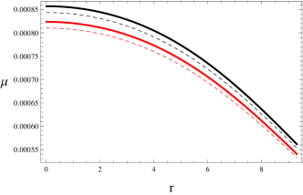
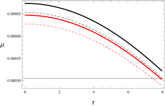
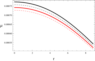
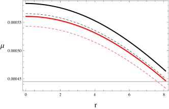
Figure 1: Plots of energy density corresponding to 4U 1820-30 (upper left), SAX J 1808.4-3658 (upper right), SMC X-4 (lower left) and Her X-I (lower right).

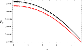
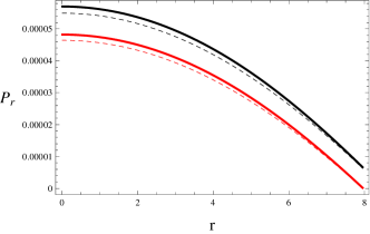
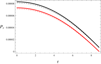
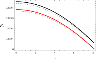
Figure 2: Plots of radial pressure corresponding to 4U 1820-30 (upper left), SAX J 1808.4-3658 (upper right), SMC X-4 (lower left) and Her X-I (lower right).

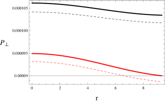
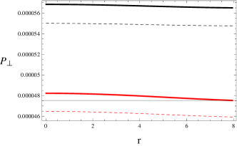
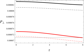
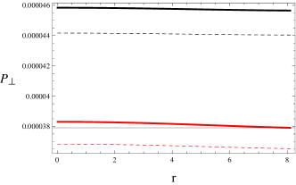
Figure 3: Plots of tangential pressure corresponding to 4U 1820-30 (upper left), SAX J 1808.4-3658 (upper right), SMC X-4 (lower left) and Her X-I (lower right).

4.2 Behavior of Anisotropy

The solution (B1)-(B3) produces the anisotropy ($\Delta=P_{\bot}-P_{r}$). We analyze the influence of charge on anisotropy to study its role in structural development. The anisotropy shows inward (decreasing) or outward (increasing) directed behavior accordingly whether the radial pressure is greater or less than the tangential component. Figure $\mathbf{4}$ depicts that it disappears at the core and possess increasing behavior in the interior of all stars. It is also shown that large value of charge reduces anisotropy.

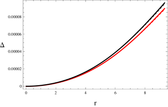
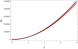
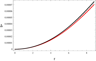
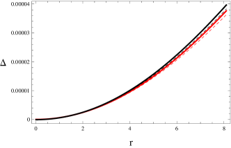
Figure 4: Plots of anisotropy corresponding to 4U 1820-30 (upper left), SAX J 1808.4-3658 (upper right), SMC X-4 (lower left) and Her X-I (lower right).

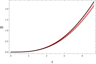
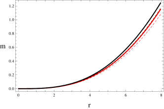
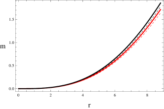
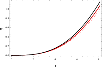
Figure 5: Plots of mass corresponding to 4U 1820-30 (upper left), SAX J 1808.4-3658 (upper right), SMC X-4 (lower left) and Her X-I (lower right).

4.3 Effective Mass, Compactness and Surface Redshift

The sphere (6) has an effective mass in terms of energy density as

$$m(r)=\frac{1}{2}\int_{0}^{\mathcal{H}}r^{2}\mu dr,$$ (38)

where $\mu$ is provided in Eq.(B1). Equivalently, Eq.(17) along with (26) yields

$$m(r)=\frac{r}{2}\left\{\frac{r^{2}\left(\bar{S}^{2}-2\bar{M}\mathcal{H}\right)e^{\frac{\left(\bar{M}\mathcal{H}-\bar{S}^{2}\right)\left(r^{2}-\mathcal{H}^{2}\right)}{\mathcal{H}^{2}\left(\mathcal{H}^{2}-2\bar{M}\mathcal{H}+\bar{S}^{2}\right)}}}{r^{2}\left(\bar{S}^{2}-2\bar{M}\mathcal{H}\right)e^{\frac{\left(\bar{M}\mathcal{H}-\bar{S}^{2}\right)\left(r^{2}-\mathcal{H}^{2}\right)}{\mathcal{H}^{2}\left(\mathcal{H}^{2}-2\bar{M}\mathcal{H}+\bar{S}^{2}\right)}}-\mathcal{H}^{2}\left(\mathcal{H}^{2}-2\bar{M}\mathcal{H}+\bar{S}^{2}\right)}\right\}.$$ (39)

The increasing behavior of mass towards boundary with respect to each candidate is shown in Figure $\mathbf{5}$ indicating that all compact objects become more massive for $\zeta=5$ and $\bar{S}=0.2$. The increment in charge results in the less massive structure. Some physical quantities play a significant role in the study of evolution of compact objects, one of them is the mass to radius ratio of a star, known as compactness. This is given as

$$\beta(r)=\frac{m(r)}{r}=\frac{1}{2}\left\{\frac{r^{2}\left(\bar{S}^{2}-2\bar{M}\mathcal{H}\right)e^{\frac{\left(\bar{M}\mathcal{H}-\bar{S}^{2}\right)\left(r^{2}-\mathcal{H}^{2}\right)}{\mathcal{H}^{2}\left(\mathcal{H}^{2}-2\bar{M}\mathcal{H}+\bar{S}^{2}\right)}}}{r^{2}\left(\bar{S}^{2}-2\bar{M}\mathcal{H}\right)e^{\frac{\left(\bar{M}\mathcal{H}-\bar{S}^{2}\right)\left(r^{2}-\mathcal{H}^{2}\right)}{\mathcal{H}^{2}\left(\mathcal{H}^{2}-2\bar{M}\mathcal{H}+\bar{S}^{2}\right)}}-\mathcal{H}^{2}\left(\mathcal{H}^{2}-2\bar{M}\mathcal{H}+\bar{S}^{2}\right)}\right\}.$$ (40)

Buchdahl [75] used the matching criteria at the hypersurface and proposed that a feasible solution corresponding to a celestial body must have its value less than $\frac{4}{9}$ everywhere. A massive object with sufficient gravitational pull undergoes certain reactions and releases electromagnetic radiations. The surface redshift quantifies increment in the wavelength of those radiations, provided as

$$D(r)=-1+\frac{1}{\sqrt{1-2\beta(r)}},$$ (41)

which then leads to

$$D(r)=-1+\sqrt{\frac{r^{2}\left(\bar{S}^{2}-2\bar{M}\mathcal{H}\right)e^{\frac{\left(\bar{M}\mathcal{H}-\bar{S}^{2}\right)\left(r^{2}-\mathcal{H}^{2}\right)}{\mathcal{H}^{2}\left(\mathcal{H}^{2}-2\bar{M}\mathcal{H}+\bar{S}^{2}\right)}}+\mathcal{H}^{2}\left(2\bar{M}\mathcal{H}-\mathcal{H}^{2}-\bar{S}^{2}\right)}{\mathcal{H}^{2}\left(2\bar{M}\mathcal{H}-\mathcal{H}^{2}-\bar{S}^{2}\right)}}.$$ (42)

For a feasible star model, Buchdahl calculated its upper limit as $2$ for isotropic interior, whereas it is $5.211$ for anisotropic configuration [81]. Figures $\mathbf{6}$ and $\mathbf{7}$ show graphs of both factors for each star that are consistent with the required range for all values of $\zeta$ and charge (Tables $\mathbf{4}-\mathbf{7}$). Moreover, these quantities increase with the increasing of bag constant and decreasing charge.

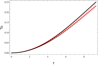
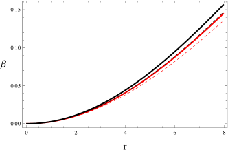
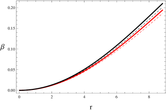
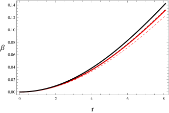
Figure 6: Plots of compactness corresponding to 4U 1820-30 (upper left), SAX J 1808.4-3658 (upper right), SMC X-4 (lower left) and Her X-I (lower right).

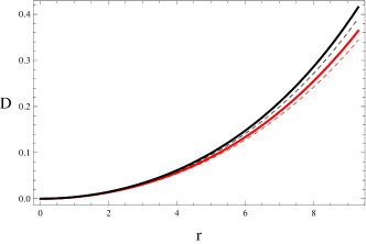
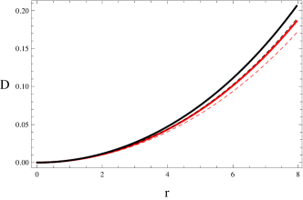
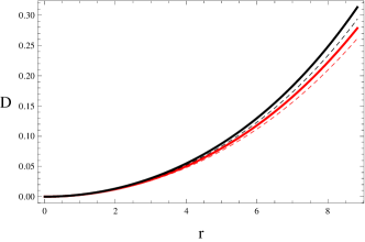
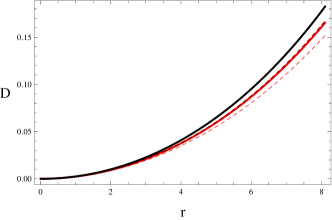
Figure 7: Plots of redshift corresponding to 4U 1820-30 (upper left), SAX J 1808.4-3658 (upper right), SMC X-4 (lower left) and Her X-I (lower right).

4.4 Energy Conditions

A geometrical structure may contain normal or exotic matter in its interior. In astrophysics, some constrains depending on state variables are extensively used, known as energy conditions. The verification of these conditions confirm the existence of normal matter in a considered star as well as viability of the developed solution. These bounds are given as

• Null: $\mu+P_{\bot}+\frac{s^{2}}{4\pi r^{4}}\geq 0$,  $\mu+P_{r}\geq 0$,

• Weak: $\mu+\frac{s^{2}}{8\pi r^{4}}\geq 0$,  $\mu+P_{\bot}+\frac{s^{2}}{4\pi r^{4}}\geq 0$,  $\mu+P_{r}\geq 0$,

• Strong: $\mu+2P_{\bot}+P_{r}+\frac{s^{2}}{4\pi r^{4}}\geq 0$,

• Dominant: $\mu-P_{\bot}\geq 0$,  $\mu-P_{r}+\frac{s^{2}}{4\pi r^{4}}\geq 0$.

We observe from the graphs of matter variables (Figures 1-3) that they possess positive behavior. Also, $\mu>P_{r}$ and $\mu>P_{\bot}$ everywhere in the domain, thus the fulfilment of all the energy conditions is obvious, contradicting the results found in [14]. However, we have not added their plots. Consequently, we can say that our resulting solution and extended model (10) are physically viable.

4.5 Tolman-Opphenheimer-Volkoff Equation

The generalized $\mathbb{TOV}$ equation is already expressed in Eq.(16). We are required to plot different forces involving in this equation to check whether the model is in stable equilibrium condition or not [47, 48]. To do this, the compact form of the non-conservation equation in the presence of charge can be written as

$$f_{g}+f_{h}+f_{a}=0,$$ (43)

where $f_{g},~{}f_{h}$ and $f_{a}$ are gravitational, hydrostatic and anisotropic forces, respectively, defined as

$$f_{g}=-\frac{\rho^{\prime}}{2}\big{(}\mu+P_{r}\big{)},$$

$$f_{h}=-\frac{dP_{r}}{dr}+\frac{ss^{\prime}}{4\pi r^{4}},$$

$$f_{a}=\frac{2}{r}\big{(}P_{\bot}-P_{r}\big{)}.$$

Here, the effective matter variables are given in Eqs.(B1)-(B3). Figure 8 exhibits the plots of this equation, from which it can clearly be noticed that our considered quark models are in hydrostatic equilibrium.

4.6 Stability Analysis

The stability criteria helps to understand the composition of astronomical structures in our universe. Here, we check stability of the developed solution through two techniques.

4.6.1 Herrera Cracking Technique

The causality condition [82] states that speed of sound in tangential and radial directions must lie within $0$ and $1$ for a stable structure, i.e., $0\leq v_{s\bot}^{2}<1$ and $0\leq v_{sr}^{2}<1$, where

$$v_{s\bot}^{2}=\frac{dP_{\bot}}{d\mu},\quad v_{sr}^{2}=\frac{dP_{r}}{d\mu}.$$ (44)

Herrera [83] suggested a cracking approach according to which the stable system must meet the condition $0\leq\mid v_{s\bot}^{2}-v_{sr}^{2}\mid<1$ everywhere in its interior. Figure $\mathbf{9}$ shows that our solution with respect to all candidates is stable throughout.

4.6.2 Adiabatic Index

Another approach to check the stability is the adiabatic index $\big{(}\Gamma\big{)}$. Several researchers [84] studied the stability of self-gravitating structures by utilizing this concept and concluded that stable models have its value not less than $\frac{4}{3}$ everywhere. Here, $\Gamma$ is defined as

$$\Gamma=\frac{\mu+P_{r}}{P_{r}}\left(\frac{dP_{r}}{d\mu}\right)=\frac{\mu+P_{r}}{P_{r}}\left(v_{sr}^{2}\right).$$ (45)

To overcome the problem such as the occurrence of dynamical instabilities inside the star, Moustakidis [85] recently proposed a critical value of the adiabatic index depending on certain parameters as

$$\Gamma_{Crit}=\frac{4}{3}+\frac{19}{21}\beta(r),$$ (46)

where the condition $\Gamma\geq\Gamma_{Crit}$ ensures the stability of compact structure. This condition has also been discussed decoupled class-one solutions [47, 48]. Figures $\mathbf{10}$ and $\mathbf{11}$ depict the plots of $\Gamma$ and $\Gamma_{Crit}$ for different values of charge corresponding to each quark star. We observe that the criterion of this approach is fulfilled and thus all the candidates show stable behavior.

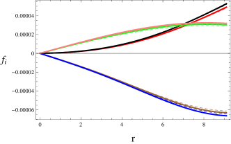
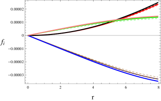
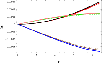
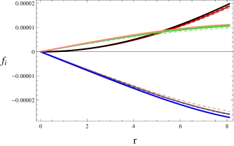
Figure 8: Plots of $f_{g}$ (blue, brown), $f_{a}$ (red, black) and $f_{h}$ (pink, green) corresponding to 4U 1820-30 (upper left), SAX J 1808.4-3658 (upper right), SMC X-4 (lower left) and Her X-I (lower right).

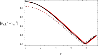
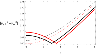
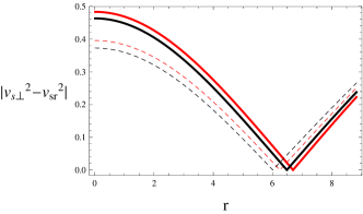
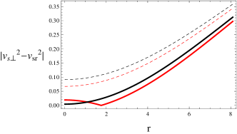
Figure 9: Plots of $|v_{s\bot}^{2}-v_{sr}^{2}|$ corresponding to 4U 1820-30 (upper left), SAX J 1808.4-3658 (upper right), SMC X-4 (lower left) and Her X-I (lower right).

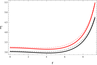
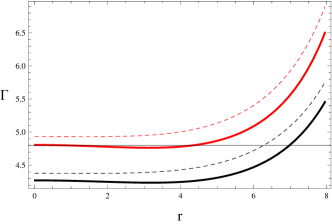
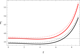
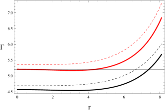
Figure 10: Plots of adiabatic index corresponding to 4U 1820-30 (upper left), SAX J 1808.4-3658 (upper right), SMC X-4 (lower left) and Her X-I (lower right).

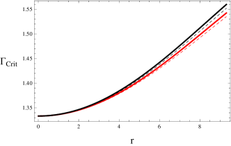
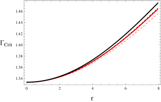
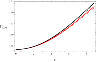
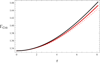
Figure 11: Plots of $\Gamma_{Crit}$ corresponding to 4U 1820-30 (upper left), SAX J 1808.4-3658 (upper right), SMC X-4 (lower left) and Her X-I (lower right).

5 Final Remarks

In this paper, we have studied the influence of matter-geometry coupling through the model $\mathcal{R}+\zeta\mathcal{Q}$ on four charged anisotropic compact stars for the coupling constant $\zeta=\pm 5$. We have adopted the matter Lagrangian proposed by Haghani et al [12] which turns out to be $\mathbb{L}_{m}=\frac{s^{2}}{2r^{4}}$. We have formulated the corresponding equations of motion and non-conservation equation. We have used the temporal metric function (25) to determine the radial metric potential (26) through embedding class-one condition and then found the solution (B1)-(B3) of the modified field equations. The four unknowns ($C_{1},C_{2},C_{3},C_{4}$) have been determined at the hypersurface with the help of observed mass and radius of each celestial object. We have used the preliminary information of four compact stars, i.e., SAX J 1808.4-3658, 4U 1820-30, SMC X-4 and Her X-I (Table $\mathbf{1}$) to calculate constants for different values of charge (Tables $\mathbf{2}$ and $\mathbf{3}$) as well as bag constant with respect to different choices of $\zeta$. We have found that the solution with respect to each star is physically acceptable as state variables are maximum (minimum) at the center (boundary). The mass of strange stars exhibits increasing behavior for the given values of charge, bag constant and $\zeta$ (Figure $\mathbf{5}$).

It is found that increasing nature of the coupling constant and decreasing the charge (i.e., $\zeta=5$ and $\bar{S}=0.2$) produce dense interiors in this modified gravity. The compactness and redshift parameters also provide acceptable behavior (Figures $\mathbf{6}$ and $\mathbf{7}$). We have obtained that our developed solution is viable and stellar models contain normal matter. Finally, we have checked hydrostatic equilibrium condition and stability of the resulting solution through two criteria. We conclude that our solution with respect to all the considered models show stable behavior for both values of charge as well as considered range of $\zeta$ (Figure $\mathbf{9}$). The adiabatic index and its critical value also confirm their stability (Figures $\mathbf{10}$ and $\mathbf{11}$). These results are observed to be consistent with [61]. It is worthwhile to mention here that all our results reduce to $\mathbb{GR}$ by choosing $\zeta=0$.

Appendix A

The explicit expressions of the matter variables are deduced from Eqs.(13)-(15) as

$$\mu =-\big{[}4r^{4}\big{(}\big{(}\chi_{3}\big{(}\zeta\chi_{6}+8\pi e^{\alpha}\big{)}-\zeta\chi_{2}\chi_{7}\big{)}\big{(}\zeta^{2}\chi_{3}\chi_{5}+\zeta\chi_{1}\big{(}\zeta\chi_{10}+8\pi e^{\alpha}\big{)}-8\pi e^{\alpha}$$

$$\times\big{(}\zeta\chi_{10}+8\pi e^{\alpha}\big{)}\big{)}+\zeta\big{(}\zeta\chi_{3}\chi_{5}+\chi_{7}\big{(}\zeta\chi_{1}-8\pi e^{\alpha}\big{)}\big{)}\big{(}\zeta\chi_{3}\chi_{9}+\chi_{2}\big{(}\zeta\chi_{10}$$

$$+8\pi e^{\alpha}\big{)}\big{)}\big{)}\big{]}^{-1}\big{[}4\zeta\big{(}\zeta\chi_{3}\chi_{9}+\chi_{2}\big{(}\zeta\chi_{10}+8\pi e^{\alpha}\big{)}\big{)}\big{(}\chi_{7}\big{(}r^{2}\big{(}r\alpha^{\prime}+e^{\alpha}-1\big{)}$$

$$+\zeta s^{2}\chi_{4}\big{)}+\chi_{3}\big{(}r^{2}\big{(}-e^{\alpha}+r\rho^{\prime}+1\big{)}+\zeta s^{2}\chi_{8}\big{)}\big{)}+\big{(}\chi_{3}\big{(}\zeta\chi_{6}+8\pi e^{\alpha}\big{)}-\zeta\chi_{2}\chi_{7}\big{)}$$

$$\big{(}-\zeta r^{4}\chi_{3}\alpha^{\prime}\rho^{\prime}+2\zeta r^{4}\chi_{3}\rho^{\prime\prime}+\zeta r^{4}\chi_{3}\rho^{\prime 2}-2\zeta r^{3}\chi_{3}\alpha^{\prime}+32\pi r^{3}e^{\alpha}\alpha^{\prime}+2\zeta r^{3}\chi_{3}\rho^{\prime}$$

$$+4\zeta r^{2}\chi_{10}\big{(}r\alpha^{\prime}+e^{\alpha}-1\big{)}-32\pi r^{2}e^{\alpha}+32\pi r^{2}e^{2\alpha}+4\zeta s^{2}\chi_{4}\big{(}\zeta\chi_{10}+8\pi e^{\alpha}\big{)}$$

$$+4\zeta^{2}s^{2}\chi_{3}\chi_{11}\big{)}\big{]},$$ (A1)

$$P_{r} =\big{[}4r^{4}\big{(}\zeta^{3}\big{(}-\chi_{3}\big{)}\chi_{5}\chi_{6}-\zeta^{3}\chi_{3}\chi_{5}\chi_{9}-8\pi\zeta^{2}\chi_{3}\chi_{5}e^{\alpha}+8\pi\zeta^{2}\chi_{7}\chi_{9}e^{\alpha}+\zeta^{2}\chi_{2}\chi_{5}$$

$$\times\big{(}\zeta\chi_{7}-\zeta\chi_{10}-8\pi e^{\alpha}\big{)}+8\pi\zeta^{2}\chi_{6}\chi_{10}e^{\alpha}-\zeta\chi_{1}\big{(}\zeta^{2}\chi_{7}\chi_{9}+\zeta\chi_{6}\big{(}\zeta\chi_{10}+8\pi e^{\alpha}\big{)}$$

$$+8\pi e^{\alpha}\big{(}\zeta\chi_{10}+8\pi e^{\alpha}\big{)}\big{)}+64\pi^{2}\zeta\chi_{6}e^{2\alpha}+64\pi^{2}\zeta\chi_{10}e^{2\alpha}+512\pi^{3}e^{3\alpha}\big{)}\big{]}^{-1}$$

$$\times\big{[}\zeta\chi_{5}\big{(}4\big{(}-\zeta\chi_{7}+\zeta\chi_{10}+8\pi e^{\alpha}\big{)}\big{(}r^{2}\big{(}r\alpha^{\prime}+e^{\alpha}-1\big{)}+\zeta s^{2}\chi_{4}\big{)}-\zeta\chi_{3}\big{(}r^{2}$$

$$\times\big{(}-2r^{2}\rho^{\prime\prime}-r^{2}\rho^{\prime 2}+r\alpha^{\prime}\big{(}r\rho^{\prime}+2\big{)}-4e^{\alpha}+2r\rho^{\prime}+4\big{)}+4\zeta s^{2}\chi_{8}-4\zeta s^{2}\chi_{11}\big{)}\big{)}$$

$$-\zeta\chi_{1}\big{(}\zeta r^{4}\chi_{7}\alpha^{\prime}\rho^{\prime}-2\zeta r^{4}\chi_{7}\rho^{\prime\prime}-\zeta r^{4}\chi_{7}\rho^{\prime 2}+2\zeta r^{3}\chi_{7}\alpha^{\prime}+32\pi r^{3}e^{\alpha}\rho^{\prime}-2\zeta r^{3}\chi_{7}\rho^{\prime}$$

$$+4\zeta r^{2}\chi_{10}\big{(}-e^{\alpha}+r\rho^{\prime}+1\big{)}+32\pi r^{2}e^{\alpha}-32\pi r^{2}e^{2\alpha}+4\zeta s^{2}\chi_{8}\big{(}\zeta\chi_{10}+8\pi e^{\alpha}\big{)}$$

$$-4\zeta^{2}s^{2}\chi_{7}\chi_{11}\big{)}-8\pi e^{\alpha}\big{(}-\zeta r^{4}\chi_{7}\alpha^{\prime}\rho^{\prime}+2\zeta r^{4}\chi_{7}\rho^{\prime\prime}+\zeta r^{4}\chi_{7}\rho^{\prime 2}-2\zeta r^{3}\chi_{7}\alpha^{\prime}$$

$$-32\pi r^{3}e^{\alpha}\rho^{\prime}+2\zeta r^{3}\chi_{7}\rho^{\prime}-4\zeta r^{2}\chi_{10}\big{(}-e^{\alpha}+r\rho^{\prime}+1\big{)}-4\zeta s^{2}\chi_{8}\big{(}\zeta\chi_{10}+8\pi e^{\alpha}\big{)}$$

$$-32\pi r^{2}e^{\alpha}+32\pi r^{2}e^{2\alpha}+4\zeta^{2}s^{2}\chi_{7}\chi_{11}\big{)}\big{]},$$ (A2)

$$P_{\bot} =\big{[}4r^{4}\big{(}\zeta^{3}\big{(}-\chi_{3}\big{)}\chi_{5}\chi_{6}-\zeta^{3}\chi_{3}\chi_{5}\chi_{9}-8\pi\zeta^{2}\chi_{3}\chi_{5}e^{\alpha}+8\pi\zeta^{2}\chi_{7}\chi_{9}e^{\alpha}+\zeta^{2}\chi_{2}\chi_{5}$$

$$\times\big{(}\zeta\chi_{7}-\zeta\chi_{10}-8\pi e^{\alpha}\big{)}+8\pi\zeta^{2}\chi_{6}\chi_{10}e^{\alpha}-\zeta\chi_{1}\big{(}\zeta^{2}\chi_{7}\chi_{9}+\zeta\chi_{6}\big{(}\zeta\chi_{10}+8\pi e^{\alpha}\big{)}$$

$$+8\pi e^{\alpha}\big{(}\zeta\chi_{10}+8\pi e^{\alpha}\big{)}\big{)}+64\pi^{2}\zeta\chi_{6}e^{2\alpha}+64\pi^{2}\zeta\chi_{10}e^{2\alpha}+512\pi^{3}e^{3\alpha}\big{)}\big{]}^{-1}$$

$$\times\big{[}\zeta\chi_{5}\big{(}\zeta\chi_{2}\big{(}r^{2}\big{(}-2r^{2}\rho^{\prime\prime}+r^{2}\big{(}-\rho^{\prime 2}\big{)}+r\alpha^{\prime}\big{(}r\rho^{\prime}+2\big{)}-4e^{\alpha}+2r\rho^{\prime}+4\big{)}$$

$$+4\zeta s^{2}\chi_{8}-4\zeta s^{2}\chi_{11}\big{)}+4\big{(}\zeta\chi_{6}+\zeta\chi_{9}+8\pi e^{\alpha}\big{)}\big{(}r^{2}\big{(}r\alpha^{\prime}+e^{\alpha}-1\big{)}+\zeta s^{2}\chi_{4}\big{)}\big{)}$$

$$+\big{(}8\pi e^{\alpha}-\zeta\chi_{1}\big{)}\big{(}\big{(}\zeta\chi_{6}+8\pi e^{\alpha}\big{)}\big{(}r^{3}\big{(}-\alpha^{\prime}\big{(}r\rho^{\prime}+2\big{)}+2r\rho^{\prime\prime}+r\rho^{\prime 2}+2\rho^{\prime}\big{)}$$

$$+4\zeta s^{2}\chi_{11}\big{)}+4\zeta\chi_{9}\big{(}r^{2}\big{(}-e^{\alpha}+r\rho^{\prime}+1\big{)}+\zeta s^{2}\chi_{8}\big{)}\big{)}\big{]},$$ (A3)

where

$$\chi_{1} =\frac{3\rho^{\prime}\alpha^{\prime}}{8}-\frac{\rho^{\prime 2}}{8}+\frac{\alpha^{\prime}}{r}+\frac{e^{\alpha}}{r^{2}}-\frac{3\rho^{\prime\prime}}{4}-\frac{3\rho^{\prime}}{2r}-\frac{1}{r^{2}},$$

$$\chi_{2} =\frac{\rho^{\prime}\alpha^{\prime}}{8}-\frac{\rho^{\prime 2}}{8}-\frac{\rho^{\prime\prime}}{4}+\frac{\alpha^{\prime}}{2r}+\frac{\alpha^{\prime\prime}}{2}-\frac{3\alpha^{\prime 2}}{4},$$

$$\chi_{3} =\frac{\alpha^{\prime}}{2r}-\frac{\rho^{\prime}}{2r}+\frac{3e^{\alpha}}{r^{2}}-\frac{1}{r^{2}},$$

$$\chi_{4} =\frac{\alpha^{\prime}}{2r}-\frac{e^{\alpha}}{2r^{2}}+\frac{1}{2r^{2}}+\frac{\rho^{\prime}\alpha^{\prime}}{8}-\frac{\rho^{\prime 2}}{8}-\frac{\rho^{\prime\prime}}{4}-\frac{e^{\alpha}}{\zeta},$$

$$\chi_{5} =\frac{\rho^{\prime}\alpha^{\prime}}{8}+\frac{\rho^{\prime 2}}{8}-\frac{\rho^{\prime\prime}}{4}-\frac{\rho^{\prime}}{2r},$$

$$\chi_{6} =\frac{5\rho^{\prime 2}}{8}-\frac{7\rho^{\prime}\alpha^{\prime}}{8}+\frac{5\rho^{\prime\prime}}{4}-\frac{7\alpha^{\prime}}{2r}+\frac{\rho^{\prime}}{r}-\alpha^{\prime 2}-\frac{e^{\alpha}}{r^{2}}+\frac{1}{r^{2}},$$

$$\chi_{7} =\frac{\alpha^{\prime}}{2r}-\frac{\rho^{\prime}}{2r}+\frac{3e^{\alpha}}{r^{2}}-\frac{1}{r^{2}},$$

$$\chi_{8} =\frac{\rho^{\prime}}{2r}+\frac{e^{\alpha}}{2r^{2}}-\frac{1}{2r^{2}}+\frac{\rho^{\prime\prime}}{4}+\frac{\rho^{\prime 2}}{8}-\frac{\rho^{\prime}\alpha^{\prime}}{8}+\frac{e^{\alpha}}{\zeta},$$

$$\chi_{9} =\frac{\rho^{\prime 2}}{8}+\frac{3\alpha^{\prime 2}}{4}-\frac{\rho^{\prime}\alpha^{\prime}}{8}+\frac{\rho^{\prime\prime}}{4}-\frac{\alpha^{\prime}}{2r}-\frac{\alpha^{\prime\prime}}{2},$$

$$\chi_{10} =\frac{\rho^{\prime 2}}{4}-\frac{\rho^{\prime}\alpha^{\prime}}{4}+\frac{\rho^{\prime\prime}}{2}-\frac{\alpha^{\prime}}{r}+\frac{\rho^{\prime}}{r},$$

$$\chi_{11} =\frac{\rho^{\prime}\alpha^{\prime}}{8}-\frac{\rho^{\prime 2}}{8}-\frac{\rho^{\prime\prime}}{4}+\frac{\alpha^{\prime}}{4r}-\frac{\rho^{\prime}}{4r}-\frac{e^{\alpha}}{\zeta}.$$

Appendix B

Equations (19)-(21) in terms of constants take the form as

$$\mu =\bigg{[}r^{4}\big{\{}16\pi\big{(}16C_{2}^{2}C_{1}C_{3}r^{2}e^{2C_{2}r^{2}}+1\big{)}^{3}-\zeta C_{2}\big{(}4096C_{2}^{5}C_{1}^{2}C_{3}^{2}r^{4}e^{4C_{2}r^{2}}\big{(}2C_{1}C_{3}$$

$$\times e^{2C_{2}r^{2}}+r^{2}\big{)}+1024C_{2}^{4}C_{1}^{2}C_{3}^{2}r^{4}e^{4C_{2}r^{2}}+64C_{2}^{3}C_{1}C_{3}r^{2}e^{2C_{2}r^{2}}\big{(}44C_{1}C_{3}e^{2C_{2}r^{2}}$$

$$+3r^{2}\big{)}-272C_{2}^{2}C_{1}C_{3}r^{2}e^{2C_{2}r^{2}}+2C_{2}\big{(}76C_{1}C_{3}e^{2C_{2}r^{2}}-3r^{2}\big{)}-23\big{)}\big{\}}\bigg{]}^{-1}$$

$$\times\bigg{[}4096\mathfrak{B}C_{2}^{6}C_{1}^{2}C_{3}^{2}r^{8}e^{4C_{2}r^{2}}\big{(}2C_{1}C_{3}e^{2C_{2}r^{2}}\big{(}8\pi r^{2}-\zeta\big{)}-\zeta r^{2}\big{)}-512C_{2}^{5}C_{1}^{2}C_{3}^{2}$$

$$\times r^{4}e^{4C_{2}r^{2}}\big{(}r^{4}(20\zeta\mathfrak{B}-6)-3\zeta s^{2}\big{)}+128C_{2}^{4}C_{1}^{2}C_{3}^{2}r^{2}e^{4C_{2}r^{2}}\big{\{}3\zeta s^{2}+96\pi\mathfrak{B}r^{6}$$

$$+r^{4}(6-40\zeta\mathfrak{B})\big{\}}-16C_{2}^{3}C_{1}C_{3}r^{2}e^{2C_{2}r^{2}}\big{(}2r^{4}(14\zeta\mathfrak{B}-9)-9\zeta s^{2}\big{)}+8C_{2}^{2}$$

$$\times\big{\{}C_{1}C_{3}e^{2C_{2}r^{2}}\big{(}3\zeta s^{2}+96\pi\mathfrak{B}r^{6}+r^{4}(6-40\zeta\mathfrak{B})\big{)}+3\zeta\mathfrak{B}r^{6}\big{\}}+C_{2}\big{\{}3\zeta s^{2}$$

$$+r^{4}(20\zeta\mathfrak{B}+6)\big{\}}+16\pi\mathfrak{B}r^{4}\bigg{]},$$ (B1)

$$P_{r} =-\bigg{[}r^{4}\big{\{}16\pi\big{(}16C_{2}^{2}C_{1}C_{3}r^{2}e^{2C_{2}r^{2}}+1\big{)}^{3}-\zeta C_{2}\big{(}4096C_{2}^{5}C_{1}^{2}C_{3}^{2}r^{4}e^{4C_{2}r^{2}}\big{(}2C_{1}$$

$$\times C_{3}e^{2C_{2}r^{2}}+r^{2}\big{)}+1024C_{2}^{4}C_{1}^{2}C_{3}^{2}r^{4}e^{4C_{2}r^{2}}+64C_{2}^{3}C_{1}C_{3}r^{2}e^{2C_{2}r^{2}}\big{(}44C_{1}e^{2C_{2}r^{2}}$$

$$\times C_{3}+3r^{2}\big{)}-272C_{2}^{2}C_{1}C_{3}r^{2}e^{2C_{2}r^{2}}+2C_{2}\big{(}76C_{1}C_{3}e^{2C_{2}r^{2}}-3r^{2}\big{)}-23\big{)}\big{\}}\bigg{]}^{-1}$$

$$\times\bigg{[}\big{(}16r^{2}C_{2}^{2}C_{1}C_{3}e^{2C_{2}r^{2}}+1\big{)}\big{(}256C_{2}^{4}\mathfrak{B}C_{1}C_{3}r^{6}e^{2C_{2}r^{2}}\big{(}2C_{1}e^{2C_{2}r^{2}}\big{(}8\pi r^{2}-\zeta\big{)}$$

$$\times C_{3}-\zeta r^{2}\big{)}+32C_{2}^{3}C_{1}C_{3}r^{2}e^{2C_{2}r^{2}}\big{(}r^{4}(4\zeta\mathfrak{B}-2)-\zeta s^{2}\big{)}+8C_{2}^{2}C_{1}C_{3}e^{2C_{2}r^{2}}$$

$$\times\big{(}64\pi\mathfrak{B}r^{6}-\zeta s^{2}-2r^{4}(6\zeta\mathfrak{B}+1)\big{)}+C_{2}\big{(}r^{4}(24\zeta\mathfrak{B}-2)-\zeta s^{2}\big{)}+16\pi\mathfrak{B}r^{4}\big{)}\bigg{]},$$ (B2)

$$P_{\bot} =\bigg{[}r^{4}\big{(}16C_{2}^{2}C_{1}C_{3}r^{2}e^{2C_{2}r^{2}}+1\big{)}^{2}\big{(}4\pi\big{(}16C_{2}^{2}C_{1}C_{3}r^{2}e^{2C_{2}r^{2}}+1\big{)}^{2}-\zeta C_{2}\big{(}8C_{2}C_{1}$$

$$\times C_{3}e^{2C_{2}r^{2}}-1\big{)}\big{(}16C_{2}^{2}C_{1}C_{3}r^{2}e^{2C_{2}r^{2}}+2C_{2}r^{2}+3\big{)}\big{)}\big{(}16\pi\big{(}16C_{2}^{2}C_{1}C_{3}r^{2}e^{2C_{2}r^{2}}$$

$$+1\big{)}^{3}-\zeta C_{2}\big{(}4096C_{2}^{5}C_{1}^{2}C_{3}^{2}r^{4}e^{4C_{2}r^{2}}\big{(}2C_{1}C_{3}e^{2C_{2}r^{2}}+r^{2}\big{)}+1024C_{2}^{4}C_{1}^{2}C_{3}^{2}r^{4}$$

$$\times e^{4C_{2}r^{2}}+64C_{2}^{3}C_{1}C_{3}r^{2}e^{2C_{2}r^{2}}\big{(}44C_{1}C_{3}e^{2C_{2}r^{2}}+3r^{2}\big{)}+2\big{(}76C_{1}C_{3}e^{2C_{2}r^{2}}-3r^{2}\big{)}$$

$$\times C_{2}-272C_{2}^{2}C_{1}C_{3}r^{2}e^{2C_{2}r^{2}}-23\big{)}\big{)}\bigg{]}^{-1}\bigg{[}-67108864C_{1}^{5}C_{3}^{5}e^{10C_{2}r^{2}}r^{10}\big{(}2C_{1}C_{3}$$

$$\times e^{2C_{2}r^{2}}\big{(}8\pi r^{2}-\zeta\big{)}-r^{2}\zeta\big{)}\big{(}\zeta\mathfrak{B}r^{6}+2C_{1}C_{3}e^{2C_{2}r^{2}}s^{2}\big{(}8\pi r^{2}-\zeta\big{)}\big{)}C_{2}^{14}-C_{1}^{5}C_{3}^{5}$$

$$\times 8388608e^{10C_{2}r^{2}}r^{10}\zeta\big{(}2\big{(}3\zeta\mathfrak{B}+80C_{1}C_{3}e^{2C_{2}r^{2}}\pi\mathfrak{B}-3\big{)}r^{6}-20C_{1}C_{3}e^{2C_{2}r^{2}}\zeta r^{4}$$

$$\times\mathfrak{B}-s^{2}\big{(}32C_{1}e^{2C_{2}r^{2}}\pi C_{3}+3\zeta\big{)}r^{2}+4C_{1}C_{3}e^{2C_{2}r^{2}}s^{2}\zeta\big{)}C_{2}^{13}-1048576C_{1}^{4}C_{3}^{4}$$

$$\times e^{8C_{2}r^{2}}r^{6}\big{(}\zeta\big{(}(2-4\zeta\mathfrak{B})r^{6}-2(1+4\pi)s^{2}\zeta r^{2}+s^{2}\zeta^{2}\big{)}r^{4}+2C_{1}C_{3}e^{2C_{2}r^{2}}\big{(}64\pi^{2}$$

$$\times s^{2}\zeta r^{4}+8\pi\big{(}2r^{8}(5\zeta\mathfrak{B}-1)-17r^{4}s^{2}\zeta\big{)}-\zeta\big{(}2(9\zeta\mathfrak{B}+5)r^{6}+s^{2}\zeta^{2}-17\zeta$$

$$\times s^{2}r^{2}\big{)}\big{)}r^{2}+8C_{1}^{2}C_{3}^{2}e^{4C_{2}r^{2}}\big{(}8\pi r^{2}-\zeta\big{)}\big{(}(6\zeta\mathfrak{B}+2)r^{6}+112\pi s^{2}r^{4}-s^{2}\zeta r^{2}$$

$$\times(21+8\pi)+s^{2}\zeta^{2}\big{)}\big{)}C_{2}^{12}-262144C_{1}^{4}C_{3}^{4}e^{8C_{2}r^{2}}r^{6}\big{(}\zeta\big{(}(94\zeta\mathfrak{B}-26)r^{6}-8$$

$$\times(4+5\pi)s^{2}\zeta r^{2}+5s^{2}\zeta^{2}\big{)}r^{2}+4C_{1}C_{3}e^{2C_{2}r^{2}}\big{(}128\pi^{2}s^{2}\zeta r^{4}+\zeta\big{(}-(44\zeta\mathfrak{B}+5)$$

$$\times r^{6}-8s^{2}\zeta r^{2}+s^{2}\zeta^{2}\big{)}+4\pi\big{(}(68\zeta\mathfrak{B}-8)r^{8}+13s^{2}\zeta r^{4}-6s^{2}\zeta^{2}r^{2}\big{)}\big{)}\big{)}C_{2}^{11}$$

$$-16384C_{1}^{2}C_{3}^{2}e^{4C_{2}r^{2}}r^{4}\big{(}-s^{2}\zeta^{3}r^{6}+C_{1}C_{3}e^{2C_{2}r^{2}}\zeta\big{(}22r^{6}-2(11+36\pi)s^{2}\zeta r^{2}$$

$$+17s^{2}\zeta^{2}\big{)}r^{4}+4C_{1}^{2}C_{3}^{2}e^{4C_{2}r^{2}}\big{(}640\pi^{2}s^{2}\zeta r^{4}-8\pi\big{(}20r^{8}+49s^{2}\zeta r^{4}+22s^{2}\zeta^{2}r^{2}\big{)}$$

$$+\zeta\big{(}4(2\zeta\mathfrak{B}+7)r^{6}+47s^{2}\zeta r^{2}+8s^{2}\zeta^{2}\big{)}\big{)}r^{2}+16C_{1}^{3}C_{3}^{3}e^{6C_{2}r^{2}}\big{(}128\pi^{2}s^{2}\big{(}42r^{2}$$

$$-5\zeta\big{)}r^{4}+8\pi\big{(}20(2\zeta\mathfrak{B}+1)r^{8}-231s^{2}\zeta r^{4}+27s^{2}\zeta^{2}r^{2}\big{)}-\zeta\big{(}4(13\zeta\mathfrak{B}+9)$$

$$\times r^{6}-154s^{2}\zeta r^{2}+17s^{2}\zeta^{2}\big{)}\big{)}\big{)}C_{2}^{10}-4096C_{1}^{2}C_{3}^{2}e^{4C_{2}r^{2}}r^{4}\big{(}-11s^{2}\zeta^{3}r^{4}+C_{1}C_{3}$$

$$\times e^{2C_{2}r^{2}}\zeta\big{(}2(274\zeta\mathfrak{B}-51)r^{6}-40(5+3\pi)s^{2}\zeta r^{2}+63s^{2}\zeta^{2}\big{)}r^{2}+4C_{1}^{2}C_{3}^{2}e^{4C_{2}r^{2}}$$

$$\times\big{(}2560\pi^{2}s^{2}\zeta r^{4}+8\pi\big{(}80(2\zeta\mathfrak{B}-1)r^{8}+254s^{2}\zeta r^{4}-129s^{2}\zeta^{2}r^{2}\big{)}+\zeta\big{(}-6$$

$$\times(32\zeta\mathfrak{B}-23)r^{6}-340s^{2}\zeta r^{2}+85s^{2}\zeta^{2}\big{)}\big{)}\big{)}C_{2}^{9}-256C_{1}C_{3}e^{2C_{2}r^{2}}r^{2}\big{(}-3s^{2}\zeta^{3}$$

$$\times r^{6}-2C_{1}C_{3}e^{2C_{2}r^{2}}\zeta\big{(}(44\zeta\mathfrak{B}-34)r^{6}+2(17+20\pi)s^{2}\zeta r^{2}+69s^{2}\zeta^{2}\big{)}r^{4}-16$$

$$\times C_{1}^{2}C_{3}^{2}e^{4C_{2}r^{2}}\big{(}-1280\pi^{2}s^{2}\zeta r^{4}-\zeta\big{(}(142-44\zeta\mathfrak{B})r^{6}+66s^{2}\zeta r^{2}+35s^{2}\zeta^{2}\big{)}$$

$$+16\pi\big{(}20(\zeta\mathfrak{B}+1)r^{8}+8s^{2}\zeta r^{4}+17s^{2}\zeta^{2}r^{2}\big{)}\big{)}r^{2}+32C_{1}^{3}C_{3}^{3}e^{6C_{2}r^{2}}\big{(}2560\pi^{2}s^{2}$$

$$\times\big{(}7r^{2}-\zeta\big{)}r^{4}+8\pi\big{(}80(\zeta\mathfrak{B}+1)r^{8}-768s^{2}\zeta r^{4}+115s^{2}\zeta^{2}r^{2}\big{)}-\zeta\big{(}2(44\zeta\mathfrak{B}$$

$$+75)r^{6}-514s^{2}\zeta r^{2}+85s^{2}\zeta^{2}\big{)}\big{)}\big{)}C_{2}^{8}-64C_{1}C_{3}e^{2C_{2}r^{2}}r^{2}\big{(}-13s^{2}\zeta^{3}r^{4}+4C_{1}C_{3}$$

$$\times e^{2C_{2}r^{2}}\zeta\big{(}50(4\zeta\mathfrak{B}-3)r^{6}+4(-13+158\pi)s^{2}\zeta r^{2}-177s^{2}\zeta^{2}\big{)}r^{2}+32C_{1}^{2}C_{3}^{2}$$

$$\times e^{4C_{2}r^{2}}\big{(}2560\pi^{2}s^{2}\zeta r^{4}+\zeta\big{(}(241-122\zeta\mathfrak{B})r^{6}-396s^{2}\zeta r^{2}+155s^{2}\zeta^{2}\big{)}+4\pi$$

$$\times\big{(}80(\zeta\mathfrak{B}-2)r^{8}+596s^{2}\zeta r^{4}-319s^{2}\zeta^{2}r^{2}\big{)}\big{)}\big{)}C_{2}^{7}-8\big{(}3s^{2}\zeta^{3}r^{6}+8C_{1}C_{3}e^{2C_{2}r^{2}}$$

$$\times\zeta^{2}\big{(}-28\mathfrak{B}r^{6}+48\pi s^{2}r^{2}+9s^{2}\zeta\big{)}r^{4}+32C_{1}^{2}C_{3}^{2}e^{4C_{2}r^{2}}\big{(}1280\pi^{2}s^{2}\zeta r^{4}+\zeta$$

$$\times\big{(}(82-174\zeta\mathfrak{B})r^{6}+160s^{2}\zeta r^{2}-123s^{2}\zeta^{2}\big{)}-8\pi\big{(}40(\zeta\mathfrak{B}+1)r^{8}-26s^{2}r^{4}$$

$$\zeta-33s^{2}\zeta^{2}r^{2}\big{)}\big{)}r^{2}+64C_{1}^{3}C_{3}^{3}e^{6C_{2}r^{2}}\big{(}2560\pi^{2}s^{2}\big{(}7r^{2}-\zeta\big{)}r^{4}+32\pi\big{(}20r^{8}-173$$

$$\times s^{2}\zeta r^{4}+25s^{2}\zeta^{2}r^{2}\big{)}+\zeta\big{(}4(10\zeta\mathfrak{B}-29)r^{6}+400s^{2}\zeta r^{2}-57s^{2}\zeta^{2}\big{)}\big{)}\big{)}C_{2}^{6}-8$$

$$\times\big{(}19s^{2}\zeta^{3}r^{4}+4C_{1}C_{3}e^{2C_{2}r^{2}}\zeta\big{(}5(2\zeta\mathfrak{B}-17)r^{6}-56s^{2}\zeta^{2}+4s^{2}\zeta(13+123\pi)$$

$$\times r^{2}\big{)}r^{2}+16C_{1}^{2}C_{3}^{2}e^{4C_{2}r^{2}}\big{(}2560\pi^{2}s^{2}\zeta r^{4}+\zeta\big{(}(235-208\zeta\mathfrak{B})r^{6}-366s^{2}\zeta r^{2}$$

$$+120s^{2}\zeta^{2}\big{)}+4\pi\big{(}40(\zeta\mathfrak{B}-4)r^{8}+644s^{2}\zeta r^{4}-299s^{2}\zeta^{2}r^{2}\big{)}\big{)}\big{)}C_{2}^{5}-2\big{(}32C_{1}^{2}$$

$$\times e^{4C_{2}r^{2}}\big{(}128\pi^{2}r^{2}\big{(}42r^{2}-5\zeta\big{)}s^{2}-4\pi\big{(}40(\zeta\mathfrak{B}-1)r^{6}+324s^{2}\zeta r^{2}-31s^{2}\zeta^{2}\big{)}$$

$$+\zeta\big{(}3(8\zeta\mathfrak{B}-5)r^{4}+59s^{2}\zeta\big{)}\big{)}C_{3}^{2}+4C_{1}e^{2C_{2}r^{2}}\big{(}1280\pi^{2}s^{2}\zeta r^{4}-32\pi\big{(}2(3\zeta\mathfrak{B}$$

$$+5)r^{8}-13s^{2}\zeta r^{4}-40s^{2}\zeta^{2}r^{2}\big{)}-\big{(}4(26\zeta\mathfrak{B}+25)r^{6}-376s^{2}\zeta r^{2}+321s^{2}\zeta^{2}\big{)}$$

$$\times\zeta\big{)}C_{3}+r^{2}\zeta\big{(}-6(2\zeta\mathfrak{B}+1)r^{6}+2(3+28\pi)s^{2}\zeta r^{2}+133s^{2}\zeta^{2}\big{)}\big{)}C_{2}^{4}-2\big{(}\zeta$$

$$\times\big{(}(20\zeta\mathfrak{B}-33)r^{6}+2(15+98\pi)s^{2}\zeta r^{2}+69s^{2}\zeta^{2}\big{)}+4C_{1}C_{3}e^{2C_{2}r^{2}}\big{(}1280\pi^{2}r^{2}$$

$$\times\zeta s^{2}+\zeta\big{(}r^{4}(73-114\zeta\mathfrak{B})-120s^{2}\zeta\big{)}+\big{(}40(\zeta\mathfrak{B}-2)r^{6}+338s^{2}\zeta r^{2}-97$$

$$\times s^{2}\zeta^{2}\big{)}4\pi\big{)}\big{)}C_{2}^{3}-\big{(}128\pi^{2}r^{2}\zeta s^{2}-8\pi\big{(}4r^{6}-7s^{2}\zeta r^{2}-35s^{2}\zeta^{2}\big{)}+32\pi e^{2C_{2}r^{2}}$$

$$\times C_{1}C_{3}\big{(}(4-8\zeta\mathfrak{B})r^{4}+224\pi s^{2}r^{2}-(31+16\pi)s^{2}\zeta\big{)}+\big{(}(42\zeta\mathfrak{B}-38)r^{4}+s^{2}$$

$$\times 73\zeta\big{)}\zeta\big{)}C_{2}^{2}-4\pi\big{(}8(\zeta\mathfrak{B}-1)r^{4}+(35+32\pi)s^{2}\zeta\big{)}C_{2}-64\pi^{2}s^{2}\bigg{]}.$$ (B3)

Appendix C

The resulting solution (B1)-(B3) produces the anisotropy as

$$\Delta =\bigg{[}r^{4}\big{(}16C_{2}^{2}C_{1}C_{3}r^{2}e^{2C_{2}r^{2}}+1\big{)}^{2}\big{(}16\pi\big{(}16C_{2}^{2}C_{1}C_{3}r^{2}e^{2C_{2}r^{2}}+1\big{)}^{3}-\zeta C_{2}\big{(}4096$$

$$\times r^{4}C_{2}^{5}C_{1}^{2}C_{3}^{2}e^{4C_{2}r^{2}}\big{(}2C_{1}C_{3}e^{2C_{2}r^{2}}+r^{2}\big{)}+1024C_{2}^{4}C_{1}^{2}C_{3}^{2}r^{4}e^{4C_{2}r^{2}}+64C_{2}^{3}C_{1}C_{3}$$

$$\times r^{2}e^{2C_{2}r^{2}}\big{(}44C_{1}C_{3}e^{2C_{2}r^{2}}+3r^{2}\big{)}-272C_{2}^{2}C_{1}C_{3}r^{2}e^{2C_{2}r^{2}}+2\big{(}76C_{1}C_{3}e^{2C_{2}r^{2}}$$

$$-3r^{2}\big{)}C_{2}-23\big{)}\big{)}\bigg{]}^{-1}\bigg{[}\big{(}16C_{2}^{2}C_{1}C_{3}r^{2}e^{2C_{2}r^{2}}+1\big{)}^{3}\big{(}256C_{2}^{4}\mathfrak{B}C_{1}C_{3}r^{6}e^{2C_{2}r^{2}}\big{(}C_{1}C_{3}$$

$$\times 2e^{2C_{2}r^{2}}\big{(}8\pi r^{2}-\zeta\big{)}-\zeta r^{2}\big{)}+32C_{2}^{3}C_{1}C_{3}r^{2}e^{2C_{2}r^{2}}\big{(}r^{4}(4\zeta\mathfrak{B}-2)-\zeta s^{2}\big{)}+8C_{2}^{2}$$

$$\times C_{1}C_{3}e^{2C_{2}r^{2}}\big{(}64\pi\mathfrak{B}r^{6}-2r^{4}(6\zeta\mathfrak{B}+1)-\zeta s^{2}\big{)}+C_{2}\big{(}r^{4}(24\zeta\mathfrak{B}-2)-\zeta s^{2}\big{)}$$

$$+16\pi r^{4}\mathfrak{B}\big{)}-\bigg{\{}4\pi\big{(}16C_{2}^{2}C_{1}C_{3}r^{2}e^{2C_{2}r^{2}}+1\big{)}^{2}-\zeta C_{2}\big{(}8C_{2}C_{1}C_{3}e^{2C_{2}r^{2}}-1\big{)}\big{(}C_{2}^{2}$$

$$\times 16C_{1}C_{3}r^{2}e^{2C_{2}r^{2}}+2C_{2}r^{2}+3\big{)}\bigg{\}}^{-1}\bigg{\{}67108864C_{1}^{5}C_{3}^{5}e^{10C_{2}r^{2}}r^{10}\big{(}2C_{1}C_{3}e^{2C_{2}r^{2}}$$

$$\times\big{(}8\pi r^{2}-\zeta\big{)}-r^{2}\zeta\big{)}\big{(}\zeta\mathfrak{B}r^{6}+2C_{1}C_{3}e^{2C_{2}r^{2}}s^{2}\big{(}8\pi r^{2}-\zeta\big{)}\big{)}C_{2}^{14}+8388608C_{1}^{5}$$

$$\times C_{3}^{5}e^{10C_{2}r^{2}}r^{10}\zeta\big{(}2\big{(}3\zeta\mathfrak{B}+80C_{1}C_{3}e^{2C_{2}r^{2}}\pi\mathfrak{B}-3\big{)}r^{6}-20C_{1}C_{3}e^{2C_{2}r^{2}}\zeta\mathfrak{B}r^{4}$$

$$-s^{2}\big{(}32C_{1}e^{2C_{2}r^{2}}\pi C_{3}+3\zeta\big{)}r^{2}+4C_{1}C_{3}e^{2C_{2}r^{2}}s^{2}\zeta\big{)}C_{2}^{13}+1048576C_{1}^{4}C_{3}^{4}e^{8C_{2}r^{2}}$$

$$\times r^{6}\big{(}\zeta\big{(}r^{6}(2-4\zeta\mathfrak{B})-2(1+4\pi)s^{2}\zeta r^{2}+s^{2}\zeta^{2}\big{)}r^{4}+2C_{1}C_{3}e^{2C_{2}r^{2}}\big{(}64\pi^{2}s^{2}\zeta r^{4}$$

$$+8\pi\big{(}2r^{8}(5\zeta\mathfrak{B}-1)-17r^{4}s^{2}\zeta\big{)}-\zeta\big{(}2(9\zeta\mathfrak{B}+5)r^{6}-17s^{2}\zeta r^{2}+s^{2}\zeta^{2}\big{)}\big{)}r^{2}$$

$$+8C_{1}^{2}C_{3}^{2}e^{4C_{2}r^{2}}\big{(}8\pi r^{2}-\zeta\big{)}\big{(}(6\zeta\mathfrak{B}+2)r^{6}+112\pi s^{2}r^{4}-(21+8\pi)s^{2}\zeta r^{2}+s^{2}$$

$$\times\zeta^{2}\big{)}\big{)}C_{2}^{12}+262144C_{1}^{4}C_{3}^{4}e^{8C_{2}r^{2}}r^{6}\big{(}\zeta r^{2}\big{(}(94\zeta\mathfrak{B}-26)r^{6}+5s^{2}\zeta^{2}-8s^{2}\zeta r^{2}(5\pi$$

$$+4)\big{)}+4C_{1}C_{3}e^{2C_{2}r^{2}}\big{(}128\pi^{2}s^{2}\zeta r^{4}+\zeta\big{(}-(44\zeta\mathfrak{B}+5)r^{6}-8s^{2}\zeta r^{2}+s^{2}\zeta^{2}\big{)}$$

$$+4\pi\big{(}(68\zeta\mathfrak{B}-8)r^{8}+13s^{2}\zeta r^{4}-6s^{2}\zeta^{2}r^{2}\big{)}\big{)}\big{)}C_{2}^{11}+16384C_{1}^{2}C_{3}^{2}e^{4C_{2}r^{2}}r^{4}$$

$$\times\big{(}-s^{2}\zeta^{3}r^{6}+C_{1}C_{3}e^{2C_{2}r^{2}}\zeta\big{(}22r^{6}-2(11+36\pi)s^{2}\zeta r^{2}+17s^{2}\zeta^{2}\big{)}r^{4}+4C_{1}^{2}C_{3}^{2}$$

$$\times e^{4C_{2}r^{2}}\big{(}640\pi^{2}s^{2}\zeta r^{4}-8\pi\big{(}20r^{8}+49s^{2}\zeta r^{4}+22s^{2}\zeta^{2}r^{2}\big{)}+\zeta\big{(}4(2\zeta\mathfrak{B}+7)r^{6}$$

$$+47s^{2}\zeta r^{2}+8s^{2}\zeta^{2}\big{)}\big{)}r^{2}+16C_{1}^{3}C_{3}^{3}e^{6C_{2}r^{2}}\big{(}128\pi^{2}s^{2}\big{(}42r^{2}-5\zeta\big{)}r^{4}+8\pi\big{(}20(2\zeta$$

$$\times\mathfrak{B}+1)r^{8}-231s^{2}\zeta r^{4}+27s^{2}\zeta^{2}r^{2}\big{)}-\zeta\big{(}4(13\zeta\mathfrak{B}+9)r^{6}-154s^{2}\zeta r^{2}+17$$

$$\times s^{2}\zeta^{2}\big{)}\big{)}\big{)}C_{2}^{10}+4096C_{1}^{2}C_{3}^{2}e^{4C_{2}r^{2}}r^{4}\big{(}-11s^{2}\zeta^{3}r^{4}+C_{1}C_{3}e^{2C_{2}r^{2}}\zeta\big{(}2r^{6}(274\zeta\mathfrak{B}$$

$$-51)-40(5+3\pi)s^{2}\zeta r^{2}+63s^{2}\zeta^{2}\big{)}r^{2}+4C_{1}^{2}C_{3}^{2}e^{4C_{2}r^{2}}\big{(}2560\pi^{2}s^{2}\zeta r^{4}+8\pi\big{(}80$$

$$\times(2\zeta\mathfrak{B}-1)r^{8}+254s^{2}\zeta r^{4}-129s^{2}\zeta^{2}r^{2}\big{)}+\zeta\big{(}-6(32\zeta\mathfrak{B}-23)r^{6}-340s^{2}$$

$$\times\zeta r^{2}+85s^{2}\zeta^{2}\big{)}\big{)}\big{)}C_{2}^{9}+256C_{1}C_{3}e^{2C_{2}r^{2}}r^{2}\big{(}-3s^{2}\zeta^{3}r^{6}-2C_{1}C_{3}e^{2C_{2}r^{2}}\zeta\big{(}(44\zeta\mathfrak{B}$$

$$-34)r^{6}+2(17+20\pi)s^{2}\zeta r^{2}+69s^{2}\zeta^{2}\big{)}r^{4}-16C_{1}^{2}C_{3}^{2}e^{4C_{2}r^{2}}\big{(}-1280\pi^{2}s^{2}\zeta r^{4}$$

$$-\zeta\big{(}(142-44\zeta\mathfrak{B})r^{6}+66s^{2}\zeta r^{2}+35s^{2}\zeta^{2}\big{)}+16\pi\big{(}20(\zeta\mathfrak{B}+1)r^{8}+8s^{2}\zeta r^{4}$$

$$+17s^{2}\zeta^{2}r^{2}\big{)}\big{)}r^{2}+32C_{1}^{3}C_{3}^{3}e^{6C_{2}r^{2}}\big{(}2560\pi^{2}s^{2}\big{(}7r^{2}-\zeta\big{)}r^{4}+8\pi\big{(}80(\zeta\mathfrak{B}+1)r^{8}$$

$$-768s^{2}\zeta r^{4}+115s^{2}\zeta^{2}r^{2}\big{)}-\zeta\big{(}2(44\zeta\mathfrak{B}+75)r^{6}-514s^{2}\zeta r^{2}+85s^{2}\zeta^{2}\big{)}\big{)}\big{)}C_{2}^{8}$$

$$+64C_{1}C_{3}e^{2C_{2}r^{2}}r^{2}\big{(}-13s^{2}\zeta^{3}r^{4}+4C_{1}C_{3}e^{2C_{2}r^{2}}\zeta\big{(}50(4\zeta\mathfrak{B}-3)r^{6}+(158\pi-13)$$

$$\times 4s^{2}\zeta r^{2}-177s^{2}\zeta^{2}\big{)}r^{2}+32C_{1}^{2}C_{3}^{2}e^{4C_{2}r^{2}}\big{(}2560\pi^{2}s^{2}\zeta r^{4}+\zeta\big{(}(241-122\zeta\mathfrak{B})r^{6}$$

$$-396s^{2}\zeta r^{2}+155s^{2}\zeta^{2}\big{)}+4\pi\big{(}80(\zeta\mathfrak{B}-2)r^{8}+596s^{2}\zeta r^{4}-319s^{2}\zeta^{2}r^{2}\big{)}\big{)}\big{)}C_{2}^{7}$$

$$+8\big{(}3s^{2}\zeta^{3}r^{6}+8C_{1}C_{3}e^{2C_{2}r^{2}}\zeta^{2}\big{(}-28\mathfrak{B}r^{6}+48\pi s^{2}r^{2}+9s^{2}\zeta\big{)}r^{4}+32e^{4C_{2}r^{2}}C_{1}^{2}$$

$$\times C_{3}^{2}\big{(}1280\pi^{2}s^{2}\zeta r^{4}+\zeta\big{(}(82-174\zeta\mathfrak{B})r^{6}+160s^{2}\zeta r^{2}-123s^{2}\zeta^{2}\big{)}-8\pi\big{(}40(\zeta$$

$$\times\mathfrak{B}+1)r^{8}-26s^{2}\zeta r^{4}-33s^{2}\zeta^{2}r^{2}\big{)}\big{)}r^{2}+64C_{1}^{3}C_{3}^{3}e^{6C_{2}r^{2}}\big{(}2560\pi^{2}s^{2}\big{(}7r^{2}-\zeta\big{)}$$

$$\times r^{4}+32\pi\big{(}20r^{8}-173s^{2}\zeta r^{4}+25s^{2}\zeta^{2}r^{2}\big{)}+\zeta\big{(}4(10\zeta\mathfrak{B}-29)r^{6}+400s^{2}\zeta r^{2}$$

$$-57s^{2}\zeta^{2}\big{)}\big{)}\big{)}C_{2}^{6}+8\big{(}19s^{2}\zeta^{3}r^{4}+4C_{1}C_{3}e^{2C_{2}r^{2}}\zeta\big{(}5(2\zeta\mathfrak{B}-17)r^{6}+4s^{2}\zeta r^{2}(13$$

$$+123\pi)-56s^{2}\zeta^{2}\big{)}r^{2}+16C_{1}^{2}C_{3}^{2}e^{4C_{2}r^{2}}\big{(}2560\pi^{2}s^{2}\zeta r^{4}+\zeta\big{(}(235-208\zeta\mathfrak{B})r^{6}$$

$$-366s^{2}\zeta r^{2}+120s^{2}\zeta^{2}\big{)}+4\pi\big{(}40(\zeta\mathfrak{B}-4)r^{8}+644s^{2}\zeta r^{4}-299s^{2}\zeta^{2}r^{2}\big{)}\big{)}\big{)}C_{2}^{5}$$

$$+2\big{(}32C_{1}^{2}e^{4C_{2}r^{2}}\big{(}128\pi^{2}r^{2}\big{(}42r^{2}-5\zeta\big{)}s^{2}-4\pi\big{(}40(\zeta\mathfrak{B}-1)r^{6}+324s^{2}\zeta r^{2}$$

$$-31s^{2}\zeta^{2}\big{)}+\zeta\big{(}3(8\zeta\mathfrak{B}-5)r^{4}+59s^{2}\zeta\big{)}\big{)}C_{3}^{2}+4C_{1}e^{2C_{2}r^{2}}\big{(}1280\pi^{2}s^{2}\zeta r^{4}-32\pi$$

$$\times\big{(}2(3\zeta\mathfrak{B}+5)r^{8}-13s^{2}\zeta r^{4}-40s^{2}\zeta^{2}r^{2}\big{)}-\zeta\big{(}4(26\zeta\mathfrak{B}+25)r^{6}-376s^{2}\zeta r^{2}$$

$$+321s^{2}\zeta^{2}\big{)}\big{)}C_{3}+r^{2}\zeta\big{(}-6(2\zeta\mathfrak{B}+1)r^{6}+2(3+28\pi)s^{2}\zeta r^{2}+133s^{2}\zeta^{2}\big{)}\big{)}C_{2}^{4}$$

$$+2\big{(}\zeta\big{(}(20\zeta\mathfrak{B}-33)r^{6}+2(15+98\pi)s^{2}\zeta r^{2}+69s^{2}\zeta^{2}\big{)}+4C_{1}C_{3}e^{2C_{2}r^{2}}\big{(}1280\pi^{2}$$

$$\times r^{2}\zeta s^{2}+\zeta\big{(}r^{4}(73-114\zeta\mathfrak{B})-120s^{2}\zeta\big{)}+4\pi\big{(}40(\zeta\mathfrak{B}-2)r^{6}+338s^{2}\zeta r^{2}$$

$$-97s^{2}\zeta^{2}\big{)}\big{)}\big{)}C_{2}^{3}+\big{(}128\pi^{2}r^{2}\zeta s^{2}-8\pi\big{(}4r^{6}-7s^{2}\zeta r^{2}-35s^{2}\zeta^{2}\big{)}+32C_{1}C_{3}e^{2C_{2}r^{2}}$$

$$\times\pi\big{(}(4-8\zeta\mathfrak{B})r^{4}+224\pi s^{2}r^{2}-(31+16\pi)s^{2}\zeta\big{)}+\zeta\big{(}(42\zeta\mathfrak{B}-38)r^{4}+73s^{2}$$

$$\times\zeta\big{)}\big{)}C_{2}^{2}+4\pi\big{(}8(\zeta\mathfrak{B}-1)r^{4}+(35+32\pi)s^{2}\zeta\big{)}C_{2}+64\pi^{2}s^{2}\bigg{\}}\bigg{]}.$$ (C1)

References

• [1] Buchdahl H A 1970 Mon. Not. R. Astron. Soc. 150 1
• [2] Nojiri S and Odintsov S D 2003 Phys. Rev. D 68 123512
• [3] Song Y S, Hu W and Sawicki I 2007 Phys. Rev. D 75 044004
• [4] Sharif M and Yousaf Z 2013 Mon. Not. R. Astron. Soc. 434 2529
• [5] Astashenok A V, Capozziello S and Odintsov S D 2014 Phys. Rev. D 89 103509
• [6] Bertolami O et al 2007 Phys. Rev. D 75 104016
• [7] Harko T et al 2011 Phys. Rev. D 84 024020
• [8] Sharif M and Zubair M 2013 J. Exp. Theor. Phys. 117 248
• [9] Shabani H and Farhoudi M 2013 Phys. Rev. D 88 044048
• [10] Sharif M and Siddiqa A 2017 Eur. Phys. J. Plus 132 529
• [11] Das A et al 2017 Phys. Rev. D 95 124011
• [12] Haghani Z et al 2013 Phys. Rev. D 88 044023
• [13] Sharif M and Zubair M 2013 J. Cosmol. Astropart. Phys. 11 042
• [14] Sharif M and Zubair M 2013 J. High Energy Phys. 12 079
• [15] Odintsov S D and SΓ‘ez-GΓ³mez D 2013 Phys. Lett. B 725 437
• [16] Baffou E H, Houndjo M J S and Tosssa J 2016 Astrophys. Space Sci. 361 376
• [17] Sharif M and Waseem A 2016 Eur. Phys. J. Plus 131 190
• [18] Sharif M and Waseem A 2016 Can. J. Phys. 94 1024
• [19] Yousaf Z, Bhatti M Z and Naseer T 2020 Eur. Phys. J. Plus 135 353
• [20] Yousaf Z, Bhatti M Z and Naseer T 2020 Phys. Dark Universe 28 100535
• [21] Yousaf Z, Bhatti M Z and Naseer T 2020 Int. J. Mod. Phys. D 29 2050061
• [22] Yousaf Z, Bhatti M Z and Naseer T 2020 Ann. Phys. 420 168267
• [23] Yousaf Z et al 2020 Phys. Dark Universe 29 100581
• [24] Yousaf Z et al 2020 Mon. Not. R. Astron. Soc. 495 4334
• [25] Sharif M and Naseer T 2021 Chin. J. Phys. 73 179
• [26] Sharif M and Naseer T 2022 Phys. Scr. 97 055004
• [27] Sharif M and Naseer T 2022 Pramana 96 119
• [28] Sharif M and Naseer T 2022 Int. J. Mod. Phys. D 31 2240017
• [29] Naseer T and Sharif M 2022 Universe 8 62
• [30] Sharif M and Naseer T 2022 Chin. J. Phys. 77 2655
• [31] Sharif M and Naseer T 2022 Eur. Phys. J. Plus 137 947
• [32] Das B et al 2011 Int. J. Mod. Phys. D 20 1675
• [33] Sunzu J M, Maharaj S D and Ray S 2014 Astrophys. Space Sci. 352 719
• [34] Gupta Y K and Maurya S K 2011 Astrophys. Space Sci. 332 155
• [35] Sharif M and Sadiq S 2016 Eur. Phys. J. C 76 568
• [36] Sharif M and Majid A 2021 Phys. Dark Universe 32 100803
• [37] Bordbar G H and Peivand A R 2011 Res. Astron. Astrophys. 11 851
• [38] Haensel P, Zdunik J L and Schaefer R 1986 Astron. Astrophys. 160 121
• [39] Cheng K S, Dai Z G and Lu T 1998 Int. J. Mod. Phys. D 7 139
• [40] Mak M K and Harko T 2002 Chin. J. Astron. Astrophys. 2 248
• [41] Demorest P B et al (2010) Nature 467 1081
• [42] Rahaman F et al 2014 Eur. Phys. J. C 74 3126
• [43] Bhar P et al 2016 Eur. Phys. J. A 52 312
• [44] Maurya S K et al 2016 Eur. Phys. J. C 76 266
• [45] Maurya S K et al 2016 Eur. Phys. J. C 76 693
• [46] Singh K N, Bhar P and Pant N 2016 Astrophys. Space Sci. 361 339
• [47] Tello-Ortiz F, Maurya S K and Gomez-Leyton Y 2020 Eur. Phys. J. C 80 324
• [48] Dayanandan B, Smitha T T and Maurya S K 2021 Phys. Scr. 96 125041
• [49] Singh K N et al 2020 Chinese Phys. C 44 105106
• [50] Rahaman M et al 2020 Eur. Phys. J. Plus 80 272
• [51] Deb D et al 2019 Mon. Not. R. Astron. Soc. 485 5652
• [52] Maurya S K et al 2019 Phys. Rev. D 100 044014
• [53] Mustafa G et al 2020 Chin. J. Phys. 67 576
• [54] Maurya S K et al 2020 Eur. Phys. J. Plus 135 824
• [55] Mustafa G et al 2021 Phys. Dark Universe 31 100747
• [56] Maurya S K, Tello-Ortiz F and Ray S 2021 Phys. Dark Universe 31 100753
• [57] Mustafa G et al 2021 Eur. Phys. J. Plus 136 166
• [58] Maurya S K, Singh K N and Nag R 2021 Chin. J. Phys. 74 313
• [59] Adnan M et al 2022 Int. J. Mod. Phys. D 19 2250073
• [60] Sarkar S, Sarkar N and Rahaman F 2022 Chin. J. Phys. 77 2028
• [61] Sharif M and Waseem A 2018 Eur. Phys. J. C 78 868
• [62] Sharif M and Majid A 2020 Eur. Phys. J. Plus 135 558
• [63] Sharif M and Saba S 2020 Chin. J. Phys. 64 374
• [64] Misner C W and Sharp D H 1964 Phys. Rev. 136 B571
• [65] Kalam M et al 2013 Int. J. Theor. Phys. 52 3319
• [66] ArbaΓ±il J D V and Malheiro M 2016 J. Cosmol. Astropart. Phys. 11 012
• [67] Biswas S et al 2019 Ann. Phys. 409 167905
• [68] Sharif M and Ramzan A 2020 Phys. Dark Universe 30 100737
• [69] Eiesland J 1925 Trans. Am. Math. Soc. 27 213
• [70] Lake K 2003 Phys. Rev. D 67 104015
• [71] Darmois G 1927 Les equations de la gravitation einsteinienne
• [72] Lichnerowicz A 1955 ThΓ©ories Relativistes de la Gravitation et de l’ElectromagnΓ©tisme Masson, Paris
• [73] Lake K 2017 Gen. Relativ. Gravit. 49 134
• [74] Dey M et al 1998 Phys. Lett. B 438 123
• [75] Buchdahl H A 1959 Phys. Rev. 116 1027
• [76] Farhi E and Jaffe R L 1984 Phys. Rev. D 30 2379
• [77] Alcock C, Farhi E and Olinto A 1986 Astrophys. J. 310 261
• [78] Gangopadhyay T et al 2013 Mon. Not. R. Astron. Soc. 431 3216
• [79] Deb D et al 2019 J. Cosmol. Astropart. Phys. 10 070
• [80] de Felice F, Yu Y and Fang J 1995 Mon. Not. R. Astron. Soc. 277 L17
• [81] Ivanov B V 2002 Phys. Rev. D 65 104011
• [82] Abreu H, Hernandez H and Nunez L A 2007 Class. Quantum Gravit. 24 4631
• [83] Herrera L 1992 Phys. Lett. A 165 206
• [84] Heintzmann H and Hillebrandt W 1975 Astron. Astrophys. 38 51
• [85] Moustakidis C C 2017 Gen. Relativ. Gravit. 49 68