Two-Sample and Change-Point Inference for Non-Euclidean Valued Time Series

Abstract

Data objects taking value in a general metric space have become increasingly common in modern data analysis. In this paper, we study two important statistical inference problems, namely, two-sample testing and change-point detection, for such non-Euclidean data under temporal dependence. Typical examples of non-Euclidean valued time series include yearly mortality distributions, time-varying networks, and covariance matrix time series. To accommodate unknown temporal dependence, we advance the self-normalization (SN) technique (Shao, 2010) to the inference of non-Euclidean time series, which is substantially different from the existing SN-based inference for functional time series that reside in Hilbert space (Zhang et al., 2011). Theoretically, we propose new regularity conditions that could be easier to check than those in the recent literature, and derive the limiting distributions of the proposed test statistics under both null and local alternatives. For change-point detection problem, we also derive the consistency for the change-point location estimator, and combine our proposed change-point test with wild binary segmentation to perform multiple change-point estimation. Numerical simulations demonstrate the effectiveness and robustness of our proposed tests compared with existing methods in the literature. Finally, we apply our tests to two-sample inference in mortality data and change-point detection in cryptocurrency data.

1 Introduction

Statistical analysis of non-Euclidean data that reside in a metric space is gradually emerging as an important branch of functional data analysis, motivated by increasing encounter of such data in many modern applications. Examples include the analysis of sequences of age-at-death distributions over calendar years (Mazzuco & Scarpa, 2015; Shang & Hyndman, 2017), covariance matrices in the analysis of diffusion tensors in medical imaging (Dryden et al., 2009), and graph Laplacians of networks (Ginestet et al., 2017). One of the main challenges in dealing with such data is that the usual vector/Hilbert space operation, such as projection and inner product may not be well defined and only the distance between two non-Euclidean data objects is available.

Despite the challenge, the list of papers that propose new statistical techniques to analyze non-Euclidean data has been growing. Building on Fréchet mean and variance (Fréchet, 1948), which are counterparts of mean and variance for metric space valued random object, Dubey & Müller (2019) proposed a test for comparing $N(\geq 2)$ populations of metric space valued data. Dubey & Müller (2020a) developed a novel test to detect a change point in the Fréchet mean and/or variance in a sequence of independent non-Euclidean data. The classical linear and nonparametric regression has also been extended to metric spaced valued data; see Petersen & Müller (2019), Tucker et al. (2022), and Zhang et al. (2021), among others. So far, the majority of the literature on non-Euclidean data has been limited to independent data, and the only exceptions are Zhang et al. (2022) and Zhu & Müller (2021, 2022), which mainly focused on the autoregressive modeling of non-Euclidean valued time series. To the best of our knowledge, no inferential tools are available for non-Euclidean valued time series in the literature.

In this paper, we address two important problems: two-sample testing and change-point detection, in the analysis of non-Euclidean valued time series. These two problems are also well motivated by the data we analyzed in the paper, namely, the yearly age-at-death distributions for countries in Europe and daily Pearson correlation matrices for five cryptocurrencies. For time series data, serial dependence is the rule rather than the exception. This motivates us to develop new tests for non-Euclidean time series that is robust to temporal dependence. Note that the two testing problems have been addressed by Dubey & Müller (2019) and Dubey & Müller (2020a), respectively for independent non-Euclidean data, but as expected, their tests fail to control the size when there is temporal dependence in the series; see Section 5 for simulation evidence.

To accommodate unknown temporal dependence, we develop test statistics based on self-normalization (Shao, 2010; Shao & Zhang, 2010), which is a nascent inferential technique for time series data. It has been mainly developed for vector time series and has been extended to functional time series in Hilbert space (Zhang et al., 2011; Zhang & Shao, 2015). The functional extension is however based on reducing the infinite dimensional functional data to finite dimension via functional principal component analysis, and then applying SN to the finite-dimensional vector time series. Such SN-based inference developed for time series in Hilbert space cannot be applied to non-Euclidean valued time series, since the projection and inner product commonly used for data in Hilbert space are not available for data objects that live in a general metric space. The SN-based extension to non-Euclidean valued time series is therefore fairly different from that in Zhang et al. (2011) and Zhang & Shao (2015), in terms of both methodology and theory. For independent non-Euclidean valued data, Dubey & Müller (2019, 2020a) build on the empirical process theory (van der Vaart & Wellner, 1996) by regulating the complexity of the analyzed metric space, which is in general abstract and may not be easy to verify. In our paper, we take a different approach that is inspired by the M-estimation theory in Pollard (1985) and Hjort & Pollard (2011) for Euclidean data, and extend it to non-Euclidean setting. We assume that the metric distance between data and the estimator of the Fréchet mean admits certain decomposition, which includes a bias term, a leading stochastic term, and a remainder term. Our technical assumptions are more intuitive and could be easier to check in practice. Furthermore, we are able to obtain explicit asymptotic distributions of our test statistics under the local alternatives of rate $O(n^{-1/2})$, where $n$ is the sample size, under our assumptions, whereas they seem difficult to derive under the entropy integral type conditions employed by Dubey & Müller (2019, 2020a).

The remainder of the paper is organized as follows. Section 2 provides background of non-Euclidean metric space in which random objects of interest reside in, and some basic assumptions that will be used throughout the paper. Section 3 proposes SN-based two-sample tests for non-Euclidean time series. Section 4 considers SN-based change-point tests. Numerical studies for the proposed tests are presented in Section 5, and Section 6 demonstrates the applicability of these tests through real data examples. Section 7 concludes. Proofs of all results are relegated to Appendix A. Appendix B summarizes the examples that satisfy assumptions in Section 2, and Appendix C provides simulation results for functional time series.

Some notations used throughout the paper are defined as follows. Let $\|\cdot\|$ denote the conventional Euclidean norm. Let $D[0,1]$ denote the space of functions on $[0,1]$ which are right continuous with left limits, endowed with the Skorokhod topology (Billingsley, 1968). We use $\Rightarrow$ to denote weak convergence in $D[0,1]$ or more generally in $\mathbb{R}^{m}$-valued function space $D^{m}[0,1]$, where $m\in\mathbb{N}$; $\to_{d}$ to denote convergence in distribution; and $\to_{p}$ to denote convergence in probability. A sequence of random variables $X_{n}$ is said to be $O_{p}(1)$ if it is bounded in probability. For $x\in\mathbb{R}$, define $\lfloor x\rfloor$ as the largest integer that is smaller than or equal to $x$, and $\lceil x\rceil$ as the smallest integer that is greater than or equal to $x$.

2 Preliminaries and Settings

In this paper, we consider a metric space $(\Omega,d)$ that is totally bounded, i.e. for any $\epsilon>0$, there exist a finite number of open $\epsilon$-balls whose union can cover $\Omega$. For a sequence of stationary random objects $\{Y_{t}\}_{t\in\mathbb{Z}}$ defined on $(\Omega,d)$, we follow Fréchet (1948), and define their Fréchet mean and variance by

$$\mu=\arg\min_{\omega\in\Omega}\mathbb{E}d^{2}(Y_{t},\omega),\quad V=\mathbb{E}d^{2}(Y_{t},\mu),$$ (1)

respectively. Fréchet mean extends the traditional mean in linear spaces to more general metric spaces by minimizing expected squared metric distance between the random object $Y_{t}$ and the centroid akin to the conventional mean by minimizing the expected sum of residual squares. It is particularly useful for objects that lie in abstract spaces without explicit algebraic structure. Fréchet variance, defined by such expected squared metric distance, is then used for measuring the dispersion in data.

Given finite samples $\{Y_{t}\}_{t=1}^{n}$, we define their Fréchet subsample mean and variance as

$$\begin{split}&\hat{\mu}_{[a,b]}=\arg\min_{\omega\in\Omega}\sum_{t=1+\lfloor na\rfloor}^{\lfloor nb\rfloor}d^{2}(Y_{t},\omega),\\ &\hat{V}_{[a,b]}=\frac{1}{\lfloor nb\rfloor-\lfloor na\rfloor}\sum_{t=1+\lfloor na\rfloor}^{\lfloor nb\rfloor}d^{2}(Y_{t},\hat{\mu}_{[a,b]}),\end{split}$$ (2)

where $(a,b)\in\mathcal{I}_{\eta}$, $\mathcal{I}_{\eta}=\{(a,b):0\leq a<b\leq 1,b-a\geq\eta\}$ for some trimming parameter $\eta\in(0,1)$. The case corresponding to $a=0$ and $b\geq\eta$ is further denoted as

$$\hat{\mu}_{[0,b]}=\hat{\mu}_{b},\quad\hat{V}_{[0,b]}=\hat{V}_{b},$$

with special case of $b=1$ corresponding to Fréchet sample mean and variance (Petersen & Müller, 2019), respectively.

Note that both Fréchet (subsample) mean and variance depend on the space $\Omega$ and metric distance $d$, which require further regulation for desired inferential purposes. In this paper, we do not impose independence assumptions, and our technical treatment differs substantially from those in the literature, c.f. Petersen & Müller (2019); Dubey & Müller (2019, 2020a, 2020b, 2021).

Assumption 2.1.

$\mu$ is unique, and for some $\delta>0$, there exists a constant $K>0$ such that,

$$\inf_{d(\omega,\mu)<\delta}\left\{\mathbb{E}\left(d^{2}(Y_{0},\omega)\right)-\mathbb{E}\left(d^{2}(Y_{0},\mu)\right)-Kd^{2}(\omega,\mu)\right\}\geq 0.$$

Assumption 2.2.

For any $(a,b)\in\mathcal{I}_{\eta}$, $\hat{\mu}_{[a,b]}$ exists and is unique almost surely.

Assumption 2.3.

For any $\omega\in\Omega$, and $(a,b)\in\mathcal{I}_{\eta}$, as $n\to\infty$,

$$\frac{1}{\lfloor nb\rfloor-\lfloor na\rfloor}\sum_{t=\lfloor na\rfloor+1}^{\lfloor nb\rfloor}[d^{2}(Y_{t},\omega)-\mathbb{E}d^{2}(Y_{t},\omega)]\to_{p}0.$$

Assumption 2.4.

For some constant $\sigma>0$,

$$\frac{1}{\sqrt{n}}\sum_{t=1}^{\lfloor nr\rfloor}\left(d^{2}(Y_{t},\mu)-V\right)\Rightarrow\sigma B(r),\quad r\in(0,1],$$

where $B(\cdot)$ is a standard Brownian motion.

Assumption 2.5.

Let $B_{\delta}(\mu)\subset\Omega$ be a ball of radius $\delta$ centered at $\mu$. For $\omega\in B_{\delta}(\mu)$, i.e. $d(\omega,\mu)\leq\delta$, we assume the following expansion

$$d^{2}(Y_{t},\omega)-d^{2}(Y_{t},\mu)=K_{d}d^{2}(\omega,\mu)+g(Y_{t},\omega,\mu)+R(Y_{t},\omega,\mu),\quad t\in\mathbb{Z},$$

where $K_{d}\in(0,\infty)$ is a constant, and $g(Y_{t},\omega,\mu)$ and $R(Y_{t},\omega,\mu)$ satisfy that, as $n\to\infty$,

$$\sup_{(a,b)\in\mathcal{I}_{\eta}}\sup_{\omega\in B_{\delta}(\mu)}\left|\frac{n^{-1/2}\sum_{t=\lfloor na\rfloor+1}^{\lfloor nb\rfloor}g(Y_{t},\omega,\mu)}{d(\omega,\mu)}\right|=O_{p}(1),$$

and

$$\sup_{(a,b)\in\mathcal{I}_{\eta}}\sup_{\omega\in B_{\delta}(\mu)}\left|\frac{n^{-1/2}\sum_{t=\lfloor na\rfloor+1}^{\lfloor nb\rfloor}R(Y_{t},\omega,\mu)}{d(\omega,\mu)+n^{1/2}d^{2}(\omega,\mu)}\right|\to_{p}0,$$

respectively.

Several remarks are given in order. Assumptions 2.1-2.3 are standard and similar conditions can be found in Dubey & Müller (2019, 2020a) and Petersen & Müller (2019). Assumptions 2.1 and 2.2 are adapted from Assumption (A1) in Dubey & Müller (2020a), and are required for identification purpose. In particular, Assumption 2.1 requires that the expected squared metric distance $\mathbb{E}d^{2}(Y_{t},\omega)$ can be well separated from the Fréchet variance, and the separation is quadratic in terms of the distance $d(\omega,\mu).$ Assumption 2.2 is useful for obtaining the uniform convergence of the subsample estimate of Fréchet mean, i.e., $\hat{\mu}_{[a,b]}$, which is a key ingredient in forming the self-normalizer in SN-based inference. Assumption 2.3 is a pointwise weak law of large numbers, c.f. Assumption (A2) in Dubey & Müller (2020a). Assumption 2.4 requires the invariance principle to hold to regularize the partial sum that appears in Fréchet subsample variances. Note that $d^{2}(Y_{t},\omega)$ takes value in $\mathbb{R}$ for any fixed $\omega\in\Omega$, thus both Assumption 2.3 and 2.4 could be implied by high-level weak temporal dependence conditions (e.g., strong mixing) in conventional Euclidean space, see Shao (2010, 2015) for discussions.

2.5 distinguishes our theoretical analysis from the existing literature. Its idea is inspired by Pollard (1985) and Hjort & Pollard (2011) for M-estimators. In the conventional Euclidean space, i.e. $(\Omega,d)=(\mathbb{R}^{m},\|\cdot\|)$ for $m\geq 1$, it is easy to see that the expansion in 2.5 holds with $K_{d}=1$, $g(Y_{t},\omega,\mu)=2(\mu-\omega)^{\top}(Y_{t}-\mu)$ and $R(Y_{t},\omega,\mu)\equiv 0.$ In more general cases, Assumption 2.5 can be interpreted as the expansion of $d^{2}(Y_{t},\omega)$ around the target value $d^{2}(Y_{t},\mu)$. In particular, $K_{d}d^{2}(\omega,\mu)$ can be viewed as the bias term, $g(Y_{t},\omega,\mu)$ works as the asymptotic leading term that is proportional to the distance $d(\omega,\mu)$ while $R(Y_{t},\omega,\mu)$ is the asymptotically negligible remainder term. More specifically, after suitable normalization, it reads as,

$$n^{-1/2}\sum_{t=\lfloor na\rfloor+1}^{\lfloor nb\rfloor}[d^{2}(Y_{t},\omega)-d^{2}(Y_{t},\mu)]$$

$$= \underbrace{n^{1/2}(b-a)K_{d}d^{2}(\omega,\mu)}_{\text{bias term}}+\underbrace{d(\omega,\mu)\frac{n^{-1/2}\sum_{t=\lfloor na\rfloor+1}^{\lfloor nb\rfloor}g(Y_{t},\omega,\mu)}{d(\omega,\mu)}}_{\text{stochastic term}}$$

$$+\underbrace{n^{-1/2}\sum_{t=\lfloor na\rfloor+1}^{\lfloor nb\rfloor}R(Y_{t},\omega,\mu)}_{\text{remainder term}}.$$

And the verification of this assumption can be done by analyzing each term. In comparison, existing literature, e.g. Petersen & Müller (2019), Dubey & Müller (2019, 2020a, 2021), impose assumptions on the complexity of $(\Omega,d)$. These assumptions typically involve the behaviors of entropy integral and covering numbers rooted in the empirical process theory (van der Vaart & Wellner, 1996), which are abstract and difficult to check in practice, see Propositions 1 and 2 in Petersen & Müller (2019). Assumption 2.5, on the contrary, regulates directly on the metric $d$ and could be easily checked for the examples below. Moreover, Assumption 2.5 is useful for deriving local powers of tests to be developed in this paper, see Section 3.2 and 4.2 for more details. Examples that can satisfy Assumptions 2.1-2.5 include:

• $L_{2}$ metric $d_{L}$ for $\Omega$ being the set of square integrable functions on $[0,1]$;

• 2-Wasserstein metric $d_{W}$ for $\Omega$ being the set of univariate probability distributions on $\mathbb{R}$;

• Frobenius metric $d_{F}$ for $\Omega$ being the set of square matrices, including the special cases of covariance matrices and graph Laplacians;

• log-Euclidean metric $d_{E}$ for $\Omega$ being the set of covariance matrices.

We refer to Appendix B for more details of these examples and verifications of above assumptions for them.

3 Two-Sample Testing

This section considers two-sample testing in metric space under temporal dependence. For two sequences of temporally dependent random objects $\{Y_{t}^{(1)},Y_{t}^{(2)}\}_{t\in\mathbb{Z}}$ on $(\Omega,d)$, we denote $Y_{t}^{(i)}\sim P^{(i)}$, where $P^{(i)}$ is the underlying marginal distribution of $Y_{t}^{(i)}$ with Fréchet mean and variance $\mu^{(i)}$ and $V^{(i)}$, $i=1,2$. Given finite sample observations $\{Y_{t}^{(1)}\}_{t=1}^{n_{1}}$ and $\{Y_{t}^{(2)}\}_{t=1}^{n_{2}}$, we are interested in the following two-sample testing problem,

$$\mathbb{H}_{0}:P^{(1)}=P^{(2)},~{}~{}\mbox{ v.s. }\mathbb{H}_{a}:P^{(1)}\neq P^{(2)}.$$

Let $n=n_{1}+n_{2}$, we assume two samples are balanced, i.e. $n_{1}/n\to\gamma_{1}$ and $n_{2}/n\to\gamma_{2}$ with $\gamma_{1},\gamma_{2}\in(0,1)$ and $\gamma_{1}+\gamma_{2}=1$ as $\min(n_{1},n_{2})\to\infty.$ For $r\in(0,1]$, we define their recursive Fréchet sample mean and variance by

$$\hat{\mu}^{(i)}_{r}=\arg\min_{\omega\in\Omega}\sum_{t=1}^{\lfloor rn_{i}\rfloor}d^{2}(Y_{t}^{(i)},\omega),\quad\hat{V}^{(i)}_{r}=\frac{1}{\lfloor rn_{i}\rfloor}\sum_{t=1}^{\lfloor rn_{i}\rfloor}d^{2}(Y_{t}^{(i)},\hat{\mu}^{(i)}_{r}),\quad i=1,2.$$

A natural candidate test of $\mathbb{H}_{0}$ is to compare their Fréchet sample mean and variance by contrasting $(\hat{\mu}^{(1)}_{1},\hat{V}^{(1)}_{1})$ and $(\hat{\mu}^{(2)}_{1},\hat{V}^{(2)}_{1})$. For the mean part, it is tempting to use $d(\hat{\mu}^{(1)}_{1},\hat{\mu}^{(2)}_{1})$ as the testing statistic. However, this is a non-trivial task as the limiting behavior of $d(\hat{\mu}^{(1)}_{1},\hat{\mu}^{(2)}_{1})$ depends heavily on the structure of the metric space, which may not admit conventional algebraic operations. Fortunately, both $\hat{V}^{(1)}_{1}$ and $\hat{V}^{(2)}_{1}$ take value in $\mathbb{R}$, and it is thus intuitive to compare their difference. In fact, Dubey & Müller (2019) propose the test statistic of the form

$$U_{n}=\frac{n_{1}n_{2}}{n\hat{\sigma}_{1}^{2}\hat{\sigma}_{2}^{2}}(\hat{V}^{(1)}_{1}-\hat{V}^{(2)}_{1})^{2},$$

where $\hat{\sigma}_{i}^{2}$ is a consistent estimator of $\lim_{n_{i}\to\infty}\mathrm{Var}\{\sqrt{n}(\hat{V}^{(i)}_{1}-V^{(i)})\}$, $i=1,2.$

However, $U_{n}$ requires both within-group and between-group independence, which is too stringent to be realistic for applications in this paper. When either of such independence is violated, the test may fail to control size, see Section 5 for numerical evidence. Furthermore, taking into account the temporal dependence requires replacing the variance by long-run variance, whose consistent estimation usually involves laborious tuning such as choices of kernels and bandwidths (Newey & West, 1987; Andrews, 1991). To this end, we invoke self-normalization technique to bypass the foregoing issues.

The core principle of self-normalization for the time series inference is to use an inconsistent long-run variance estimator that is a function of recursive estimates to yield an asymptotically pivotal statistic. The SN procedure does not involve any tuning parameter or involves less number of tuning parameters compared to traditional counterparts. See Shao (2015) for a comprehensive review of recent developments for low dimensional time series. For recent extension to inference for high-dimensional time series, we refer to Wang & Shao (2020) and Wang et al. (2022).

3.1 Test Statistics

Define the recursive subsample test statistic based on Fréchet variance as

$$T_{n}(r)=r(\hat{V}^{(1)}_{r}-\hat{V}^{(2)}_{r}),~{}r\in[\eta,1],$$

and then construct the SN based test statistic as

$$D_{n,1}=\frac{n\left[T_{n}(1)\right]^{2}}{\sum_{k=\lfloor n\eta\rfloor}^{n}\left[T_{n}(\frac{k}{n})-\frac{k}{n}T_{n}(1)\right]^{2}},$$ (3)

where $\eta\in(0,1)$ is a trimming parameter for controlling the estimation effect of $T_{n}(r)$ when $r$ is close to 0, which is important for deriving the uniform convergence of $\{\sqrt{n}T_{n}(r),r\in[\eta,1]\}$, see Zhou & Shao (2013) and Jiang et al. (2022) for similar technical treatments.

The testing statistic (3) is composed of the numerator $n[T_{n}(1)]^{2}$, which captures the difference in Fréchet variances, and the denominator $\sum_{k=\lfloor n\eta\rfloor}^{n}\big{[}T_{n}(\frac{k}{n})-$ $\frac{k}{n}T_{n}(1)\big{]}^{2}$, which is called self-normalizer and mimics the behavior of the numerator with suitable centering and trimming. For each $r\in[\eta,1]$, $T_{n}(r)$ is expected to be a consistent estimator for $r(V^{(1)}-V^{(2)}).$ Therefore, under $\mathbb{H}_{a}$, $T_{n}(1)$ is large when there is significant difference in Fréchet variance, whereas the key element $T_{n}(r)-rT_{n}(1)$ in self-normalizer remains to be small. This suggests that we should reject $\mathbb{H}_{0}$ for large values of $D_{n,1}$.

Note that (3) only targets at difference in Fréchet variances. To detect the difference in Fréchet means, we can use contaminated Fréchet variance (Dubey & Müller, 2020a). Let

$$\hat{V}^{C,(1)}_{r}=\frac{1}{\lfloor rn_{1}\rfloor}\sum_{t=1}^{\lfloor rn_{1}\rfloor}d^{2}(Y_{t}^{(1)},\hat{\mu}^{(2)}_{r}),\quad\text{and}\quad\hat{V}^{C,(2)}_{r}=\frac{1}{\lfloor rn_{2}\rfloor}\sum_{t=1}^{\lfloor rn_{2}\rfloor}d^{2}(Y_{t}^{(2)},\hat{\mu}^{(1)}_{r}),$$

and

$$T_{n}^{C}(r)=r(\hat{V}^{C,(1)}_{r}+\hat{V}^{C,(2)}_{r}-\hat{V}^{(1)}_{r}-\hat{V}^{(2)}_{r}).$$

The contaminated Fréchet sample variances $\hat{V}^{C,(1)}_{r}$ and $\hat{V}^{C,(2)}_{r}$ switch the role of $\hat{\mu}_{r}^{(1)}$ and $\hat{\mu}_{r}^{(2)}$ in $\hat{V}^{(1)}_{r}$ and $\hat{V}^{(2)}_{r}$, respectively, and could be viewed as proxies for measuring Fréchet mean differences.

Intuitively, it is expected that $\hat{V}^{C,(i)}_{r}\approx\mathbb{E}d^{2}(Y_{t}^{(i)},\mu^{(3-i)}),$ and $\hat{V}^{(i)}_{r}\approx\mathbb{E}d^{2}(Y_{t}^{(i)},$ $\mu^{(i)}),i=1,2$. Under $\mathbb{H}_{0}$, both $\hat{\mu}_{r}^{(1)}$ and $\hat{\mu}_{r}^{(2)}$ are consistent estimators for ${\mu}^{(1)}={\mu}^{(2)}$, thus $\hat{V}^{C,(i)}_{r}\approx\hat{V}^{(i)}_{r},i=1,2$, which indicates a small value for $T_{n}^{C}(r)$. On the contrary, when $d({\mu}^{(1)},{\mu}^{(2)})>0$, $\hat{V}^{C,(i)}_{r}$ could be much larger than $\hat{V}^{(i)}_{r}$ as $\mathbb{E}d^{2}(Y_{t}^{(i)},\mu^{(3-i)})>\mathbb{E}d^{2}(Y_{t}^{(i)},\mu^{(i)})=\arg\min_{\omega\in\Omega}\mathbb{E}d^{2}(Y_{t}^{(i)},\omega)$, $i=1,2$, resulting in large value of $T_{n}^{C}(r)$.

The power-augmented test statistic is thus defined by

$$D_{n,2}=\frac{n\left\{\left[T_{n}(1)\right]^{2}+\left[T_{n}^{C}(1)\right]^{2}\right\}}{\sum_{k=\lfloor n\eta\rfloor}^{n}\left\{\left[T_{n}(\frac{k}{n})-\frac{k}{n}T_{n}(1)\right]^{2}+\left[T_{n}^{C}(\frac{k}{n})-\frac{k}{n}T_{n}^{C}(1)\right]^{2}\right\}},$$ (4)

where the additional term $\sum_{k=\lfloor n\eta\rfloor}^{n}\left[T_{n}^{C}(\frac{k}{n})-\frac{k}{n}T_{n}^{C}(1)\right]^{2}$ that appears in the self-normalizer is used to stabilize finite sample performances.

Remark 3.1.

Our proposed tests could be adapted to comparison of $N$-sample populations (Dubey & Müller, 2019), where $N\geq 2$. An natural way of extension would be aggregating all the pairwise differences in Fréchet variance and contaminated variance. Specifically, let the $N$ groups of random data objects be $\{Y_{t}^{(i)}\}_{t=1}^{n_{i}}$, $i=1,\cdots,N$. The null hypothesis is given as

$$\mathbb{H}_{0}:P^{(1)}=\cdots=P^{(N)},$$

for some $N\geq 2$.

Let $\hat{\mu}^{(i)}_{r}$ and $\hat{V}^{(i)}_{r}$, $r\in[\eta,1]$ be the Fréchet subsample mean and variance, respectively, for the $i$th group, $i=1,\cdots,N$. For $1\leq i\neq j\leq N$, define the pairwise contaminated Fréchet subsample variance as

$$\hat{V}^{C,(i,j)}_{r}=\frac{1}{\lfloor rn_{i}\rfloor}\sum_{t=1}^{\lfloor rn_{i}\rfloor}d^{2}(Y_{t}^{(i)},\hat{\mu}^{(j)}_{r}),~{}r\in[\eta,1],$$

and define the recursive statistics

$$T_{n}^{i,j}(r)=r(\hat{V}^{(i)}_{r}-\hat{V}^{(j)}_{r}),\quad T_{n}^{C,i,j}(r)=r(\hat{V}^{C,(i,j)}_{r}+\hat{V}^{C,(j,i)}_{r}-\hat{V}^{(i)}_{r}-\hat{V}^{(j)}_{r}),~{}r\in[\eta,1].$$

In the same spirit of the test statistics $D_{n,1}$ and $D_{n,2}$, for $n=\sum_{i=1}^{N}n_{i},$ we may construct their counterparts for the $N$-sample testing problem as

$$D^{(N)}_{n,1}=\frac{n\sum_{i<j}\left[T_{n}^{i,j}(1)\right]^{2}}{\sum_{k=\lfloor n\eta\rfloor}^{n}\sum_{i<j}\left[T_{n}^{i,j}(\frac{k}{n})-\frac{k}{n}T_{n}^{i,j}(1)\right]^{2}},$$

and

$$D^{(N)}_{n,2}=\frac{n\sum_{i<j}\left\{\left[T_{n}^{i,j}(1)\right]^{2}+\left[T_{n}^{C,i,j}(1)\right]^{2}\right\}}{\sum_{k=\lfloor n\eta\rfloor}^{n}\sum_{i<j}\left\{\left[T_{n}^{i,j}(\frac{k}{n})-\frac{k}{n}T_{n}^{i,j}(1)\right]^{2}+\left[T_{n}^{C,i,j}(\frac{k}{n})-\frac{k}{n}T_{n}^{C,i,j}(1)\right]^{2}\right\}}.$$

Compared with classical $N$-sample testing problem in Euclidean spaces, e.g. analysis of variance (ANOVA), the above modification does not require Gaussianity, equal variance, or serial independence. Therefore, they could be work for broader classes of distributions. We leave out the details for the sake of space.

3.2 Asymptotic Theory

Before we present asymptotic results of the proposed tests, we need a slightly stronger assumption than Assumption 2.4 to regulate the joint behavior of partial sums for both samples.

Assumption 3.1.

For some $\sigma_{1}>0$ and $\sigma_{2}>0$, we have

$$\frac{1}{\sqrt{n}}\sum_{t=1}^{\lfloor nr\rfloor}\left(\begin{matrix}d^{2}(Y_{t}^{(1)},\mu^{(1)})-V^{(1)}\\ d^{2}(Y_{t}^{(2)},\mu^{(2)})-V^{(2)}\end{matrix}\right)\Rightarrow\left(\begin{matrix}\sigma_{1}B^{(1)}(r)\\ \sigma_{2}B^{(2)}(r)\end{matrix}\right),$$

where $B^{(1)}(\cdot)$ and $B^{(2)}(\cdot)$ are two standard Brownian motions with unknown correlation parameter $\rho\in(-1,1)$, and $\sigma_{1},\sigma_{2}\neq 0$ are unknown parameters characterizing the long-run variance.

Theorem 3.1.

Suppose Assumptions 2.1-2.5 (with 2.4 replaced by 3.1) hold for both $\{Y_{t}^{(1)}\}_{t=1}^{n_{1}}$ and $\{Y_{t}^{(2)}\}_{t=1}^{n_{2}}$. Then as $n\to\infty$, under $\mathbb{H}_{0}$, for $i=1,2$,

$$D_{n,i}\to_{d}\frac{\xi^{2}_{\gamma_{1},\gamma_{2}}(1;\sigma_{1},\sigma_{2})}{\int_{\eta}^{1}\left[\xi_{\gamma_{1},\gamma_{2}}(r;\sigma_{1},\sigma_{2})-r\xi_{\gamma_{1},\gamma_{2}}(1;\sigma_{1},\sigma_{2})\right]^{2}dr}:=\mathcal{D}_{\eta},\quad$$

where

$$\xi_{\gamma_{1},\gamma_{2}}(r;\sigma_{1},\sigma_{2})=\gamma_{1}^{-1}\sigma_{1}B^{(1)}(\gamma_{1}r)-\gamma_{2}^{-1}\sigma_{2}B^{(2)}(\gamma_{2}r).$$ (5)

Theorem 3.1 obtains the same limiting null distribution for Fréchet variance based test $D_{n,1}$ and its power-augmented version $D_{n,2}$. Although $D_{n,2}$ contains contaminated variance $T_{n}^{C}(1)$, its contribution is asymptotically vanishing as $n\to\infty$. This is an immediate consequence of the fact that

$$\sup_{r\in[\eta,1]}|\sqrt{n}T_{n}^{C}(r)|\to_{p}0,$$

see proof of Theorem 3.1 in Appendix A. Similar phenomenon has been documented in Dubey & Müller (2019) under different assumptions.

We next consider the power behavior under the Pitman local alternative,

$$\mathbb{H}_{an}:\quad V^{(1)}-V^{(2)}=n^{-\kappa_{V}}\Delta_{V},\quad\mbox{ and }\quad d^{2}(\mu^{(1)},\mu^{(2)})=n^{-\kappa_{M}}\Delta_{M},$$

with $\Delta_{V}\in\mathbb{R}$, $\Delta_{M}\in(0,\infty)$, and $\kappa_{V},\kappa_{M}\in(0,\infty).$

Theorem 3.2.

Suppose Assumptions 2.1-2.5 (with 2.4 replaced by 3.1) hold for both $\{Y_{t}^{(1)}\}_{t=1}^{n_{1}}$ and $\{Y_{t}^{(2)}\}_{t=1}^{n_{2}}$. As $n\to\infty$, under $\mathbb{H}_{an}$,

• if $\max\{\kappa_{V},\kappa_{M}\}\in(0,1/2)$, then for $i=1,2$, $D_{n,i}\to_{p}\infty$;

• if $\min\{\kappa_{V},\kappa_{M}\}\in(1/2,\infty)$, then for $i=1,2$, $D_{n,i}\to_{d}\mathcal{D}_{\eta}$;

• if $\kappa_{V}=1/2$ and $\kappa_{M}\in(1/2,\infty)$, then for $i=1,2$,

  $$D_{n,i}\to_{d}\frac{\left(\xi_{\gamma_{1},\gamma_{2}}(1;\sigma_{1},\sigma_{2})+\Delta_{V}\right)^{2}}{\int_{\eta}^{1}\left(\xi_{\gamma_{1},\gamma_{2}}(r;\sigma_{1},\sigma_{2})-r\xi_{\gamma_{1},\gamma_{2}}(1;\sigma_{1},\sigma_{2})\right)^{2}dr};$$

• if $\kappa_{V}\in(1/2,\infty)$ and $\kappa_{M}=1/2$, then $D_{n,1}\to_{d}\mathcal{D}_{\eta}$, and

  $$D_{n,2}\to_{d}\frac{\left(\xi_{\gamma_{1},\gamma_{2}}(1;\sigma_{1},\sigma_{2})\right)^{2}+4K_{d}^{2}\Delta_{M}^{2}}{\int_{\eta}^{1}\left(\xi_{\gamma_{1},\gamma_{2}}(r;\sigma_{1},\sigma_{2})-r\xi_{\gamma_{1},\gamma_{2}}(1;\sigma_{1},\sigma_{2})\right)^{2}dr};$$

• if $\kappa_{V}=\kappa_{M}=1/2$, then

  $$D_{n,1}\to_{d}\frac{\left(\xi_{\gamma_{1},\gamma_{2}}(1;\sigma_{1},\sigma_{2})+\Delta_{V}\right)^{2}}{\int_{\eta}^{1}\left(\xi_{\gamma_{1},\gamma_{2}}(r;\sigma_{1},\sigma_{2})-r\xi_{\gamma_{1},\gamma_{2}}(1;\sigma_{1},\sigma_{2})\right)^{2}dr},$$

  $$D_{n,2}\to_{d}\frac{\left(\xi_{\gamma_{1},\gamma_{2}}(1;\sigma_{1},\sigma_{2})+\Delta_{V}\right)^{2}+4K_{d}^{2}\Delta_{M}^{2}}{\int_{\eta}^{1}\left(\xi_{\gamma_{1},\gamma_{2}}(r;\sigma_{1},\sigma_{2})-r\xi_{\gamma_{1},\gamma_{2}}(1;\sigma_{1},\sigma_{2})\right)^{2}dr};$$

where $K_{d}$ is defined in Assumption 2.5.

Theorem 3.2 presents the asymptotic behaviors for both test statistics under local alternatives in various regimes. In particular, $D_{n,1}$ can detect differences in Fréchet variance at local rate $n^{-1/2}$, but possesses trivial power against Fréchet mean difference regardless of the regime of $\kappa_{M}$. In comparison, $D_{n,2}$ is powerful for differences in both Fréchet variance and Fréchet mean at local rate $n^{-1/2}$, which validates our claim that $D_{n,2}$ indeed augments power.

Our results merit additional remarks when compared with Dubey & Müller (2019). In Dubey & Müller (2019), they only obtain the consistency of their test under either $n^{1/2}|V^{(1)}-V^{(2)}|\to\infty$ or $n^{1/2}d^{2}(\mu^{(1)},\mu^{(2)})\to\infty$, while Theorem 3.2 explicitly characterizes the asymptotic distributions of our test statistics under local alternatives of order $O(n^{-1/2})$, which depend on $\kappa_{V}$ and $\kappa_{M}$. Such theoretical improvement relies crucially on our newly developed proof techniques based on Assumption 2.5, and it seems difficult to derive such limiting distributions under empirical-process-based assumptions in Dubey & Müller (2019). However, we do admit that self-normalization could result in moderate power loss compared with $t$-type test statistics, see (Shao & Zhang, 2010) for evidence in Euclidean space.

Note that the limiting distributions derived in 3.1 and 3.2 contain a key quantity $\xi_{\gamma_{1},\gamma_{2}}(r;\sigma_{1},\sigma_{2})$ defined in (5), which depends on nuisance parameters $\sigma_{1},\sigma_{2}$ and $\rho$. This may hinder the practical use of the tests. The following corollary, however, justifies the wide applicability of our tests.

Corollary 3.1.

Under Assumption 3.1, if either $\gamma_{1}=\gamma_{2}=1/2$ or $\rho=0$, then for any constants $C_{a},C_{b}\in\mathbb{R}$,

$$\frac{\left(\xi_{\gamma_{1},\gamma_{2}}(1;\sigma_{1},\sigma_{2})+C_{a}\right)^{2}+C_{b}^{2}}{\int_{\eta}^{1}\left(\xi_{\gamma_{1},\gamma_{2}}(r;\sigma_{1},\sigma_{2})-r\xi_{\gamma_{1},\gamma_{2}}(1;\sigma_{1},\sigma_{2})\right)^{2}dr}=_{d}\frac{\left(B(1)+C_{a}/C_{\xi}\right)^{2}+(C_{b}/C_{\xi})^{2}}{\int_{\eta}^{1}\left(B(r)-rB(1)\right)^{2}dr},$$

where

$$C_{\xi}=\begin{cases}\sqrt{2\sigma_{1}^{2}+2\sigma_{2}^{2}-4\rho\sigma_{1}\sigma_{2}},\quad&\text{if }\gamma_{1}=\gamma_{2},\\ \sqrt{{\sigma_{1}^{2}/\gamma_{1}}+{\sigma_{2}^{2}/\gamma_{2}}},\quad&\text{if }\rho=0.\end{cases}$$

Therefore, by choosing $C_{a}=C_{b}=0$ in 3.1, we obtain the pivotal limiting distribution

$$\mathcal{D}_{\eta}=_{d}\frac{B^{2}(1)}{\int_{\eta}^{1}\left(B(r)-rB(1)\right)^{2}dr}.$$

The asymptotic distributions in 3.2 can be similarly derived by letting either $C_{a}=\Delta_{V}$ or $C_{b}=2K_{d}\Delta_{M}$.

Therefore, when either two samples are of the same length $(\gamma_{1}=\gamma_{2})$ or two samples are asymptotically independent $(\rho=0)$, the limiting distribution $\mathcal{D}_{\eta}$ is pivotal. In practice, we reject $\mathbb{H}_{0}$ if $D_{n,i}>Q_{\mathcal{D}_{\eta}}(1-\alpha)$ where $Q_{\mathcal{D}_{\eta}}(1-\alpha)$ denotes the $1-\alpha$ quantile of (the pivotal) ${D}_{\eta}$.

In Table 1, we tabulate commonly used critical values under various choices of $\eta$ by simulating 50,000 i.i.d. $\mathcal{N}$(0,1) random variables 10,000 times and approximating a standard Brownian motion by standardized partial sum of i.i.d. $\mathcal{N}$(0,1) random variables.

Table 1: Simulated critical values $Q_{\mathcal{D}_{\eta}}(1-\alpha)$

	0.02	0.05	0.1	0.15
10%	28.51	28.88	30.02	31.87
5%	46.10	46.72	48.80	51.87
1%	101.58	103.70	108.93	116.72
0.5%	131.55	134.00	142.34	151.93

4 Change-Point Test

Inspired by the two-sample tests developed in Section 3, this section considers the change-point detection problem for a sequence of random objects $\{Y_{t}\}_{t=1}^{n}$, i.e.

$$\mathbb{H}_{0}:Y_{1},Y_{2},\ldots,Y_{n}\sim P^{(1)}$$

against the single change-point alternative,

$$\mathbb{H}_{a}:\text{ there exists }0<\tau<1\text{ such that }Y_{t}=\left\{\begin{array}[]{l}Y_{t}^{(1)}\sim P^{(1)},1\leq t\leq\lfloor n\tau\rfloor\\ Y_{t}^{(2)}\sim P^{(2)},\lfloor n\tau\rfloor+1\leq t\leq n.\end{array}\right.$$

The single change-point testing problem can be roughly viewed as two-sample testing without knowing where the two samples split, and they share certain similarities in terms of statistical methods and theory.

Recall the Fréchet subsample mean $\hat{\mu}_{[a,b]}$ and variance $\hat{V}_{[a,b]}$ in (2), we further define the pooled contaminated variance separated by $r\in(a,b)$ as

$$\hat{V}_{[r;a,b]}^{C}=\frac{1}{\lfloor nr\rfloor-\lfloor na\rfloor}\sum_{i=\lfloor na\rfloor+1}^{\lfloor nr\rfloor}d^{2}\left(Y_{i},\hat{\mu}_{[r,b]}\right)+\frac{1}{\lfloor nb\rfloor-\lfloor nr\rfloor}\sum_{i=\lfloor nr\rfloor+1}^{\lfloor nb\rfloor}d^{2}\left(Y_{i},\hat{\mu}_{[a,r]}\right).$$

Define the subsample test statistics

$$T_{n}(r;a,b)=\frac{(r-a)(b-r)}{b-a}\left(\hat{V}_{[a,r]}-\hat{V}_{[r,b]}\right),$$

and

$$T_{n}^{C}(r;a,b)=\frac{(r-a)(b-r)}{b-a}\left(\hat{V}_{[r;a,b]}^{C}-\hat{V}_{[a,r]}-\hat{V}_{[r,b]}\right).$$

Note that $T_{n}(r;a,b)$ and $T_{n}^{C}(r;a,b)$ are natural extensions of $T_{n}(r)$ and $T_{n}^{C}(r)$ from two-sample testing problem to change-point detection problem by viewing $\{Y_{t}\}_{t=\lfloor na\rfloor+1}^{\lfloor nr\rfloor}$ and $\{Y_{t}\}_{t=\lfloor nr\rfloor+1}^{\lfloor nb\rfloor}$ as two separated samples. Intuitively, the contrast statistics $T_{n}(r;a,b)$ and $T_{n}^{C}(r;a,b)$ are expected to attain their maxima (in absolute value) when $r$ is set at or close to the true change-point location $\tau$.

4.1 Test Statistics

For some trimming parameters $\eta_{1}$ and $\eta_{2}$ such that $\eta_{1}>2\eta_{2}$, and $\eta_{1}\in(0,1/2)$, in the same spirit of $D_{n,1}$ and $D_{n,2}$, and with a bit abuse of notation, we define the testing statistics

$$SN_{i}=\max_{\lfloor n\eta_{1}\rfloor\leq k\leq n-\lfloor n\eta_{1}\rfloor}D_{n,i}(k),\quad i=1,2,$$

where

$$D_{n,1}(k)= \frac{n\left[T_{n}\left(\frac{k}{n};0,1\right)\right]^{2}}{\sum_{l=\lfloor n\eta_{2}\rfloor}^{k-\lfloor n\eta_{2}\rfloor}\left[T_{n}\left(\frac{l}{n};0,\frac{k}{n}\right)\right]^{2}+\sum_{l=k+\lfloor n\eta_{2}\rfloor}^{n-\lfloor n\eta_{2}\rfloor}\left[T_{n}\left(\frac{l}{n};\frac{k}{n},1\right)\right]^{2}},$$

$$D_{n,2}(k)= \frac{n\left\{\left[T_{n}\left(\frac{k}{n};0,1\right)\right]^{2}+\left[T_{n}^{C}\left(\frac{k}{n};0,1\right)\right]^{2}\right\}}{L_{n}(k)+R_{n}(k)},$$

with

$$L_{n}(k)= \sum_{l=\lfloor n\eta_{2}\rfloor}^{k-\lfloor n\eta_{2}\rfloor}\left\{\left[T_{n}\left(\frac{l}{n};0,\frac{k}{n}\right)\right]^{2}+\left[T^{C}_{n}\left(\frac{l}{n};0,\frac{k}{n}\right)\right]^{2}\right\},$$

$$R_{n}(k)= \sum_{l=k+\lfloor n\eta_{2}\rfloor}^{n-\lfloor n\eta_{2}\rfloor}\left\{\left[T_{n}\left(\frac{l}{n};\frac{k}{n},1\right)\right]^{2}+\left[T^{C}_{n}\left(\frac{l}{n};\frac{k}{n},1\right)\right]^{2}\right\}.$$

The trimming parameter $\eta_{1}$ plays a similar role as $\eta$ in two-sample testing problem for stabilizing the estimation effect for relatively small sample sizes, while the additional trimming $\eta_{2}$ is introduced to ensure that the subsample estimates in the self-normalizers are constructed with the subsample size proportional to $n$. Furthermore, we note that the self-normalizers here are modified to accommodate for the unknown change-point location, see Shao & Zhang (2010), Zhang & Lavitas (2018) for more discussion.

4.2 Asymptotic Theory

Theorem 4.1.

Suppose Assumptions 2.1-2.5 hold. Then, under $\mathbb{H}_{0}$, we have for $i=1,2$,

$$SN_{i}=\max_{\lfloor n\eta_{1}\rfloor\leq k\leq n-\lfloor n\eta_{1}\rfloor}D_{n,i}(k)\Rightarrow\sup_{r\in[\eta_{1},1-\eta_{1}]}\frac{[B(r)-rB(1)]^{2}}{V(r,\eta)}:=\mathcal{S}_{\eta},$$

where $V(r,\eta)=\int_{\eta_{2}}^{r-\eta_{2}}[B(u)-u/rB(r)]^{2}du+\int_{r+\eta_{2}}^{1-\eta_{2}}[B(1)-B(u)-(1-u)/(1-r)\{B(1)-B(r)\}]^{2}du$.

Similar to Theorem 3.1, Theorem 4.1 states that both change-point test statistics have the same pivotal limiting null distribution $\mathcal{S}_{\eta}$. The test is thus rejected when $SN_{i}>Q_{\mathcal{S}_{\eta}}(1-\alpha)$, $i=1,2$, where $Q_{\mathcal{S}_{\eta}}(1-\alpha)$ denotes the $1-\alpha$ quantile of $\mathcal{S}_{\eta}$. In Table 2, we tabulate commonly used critical values under various choices of $(\eta_{1},\eta_{2})$ by simulations.

Table 2: Simulated critical values $Q_{\mathcal{S}_{\eta}}(1-\alpha)$

	(0.02,0.05)	(0.04,0.1)	(0.05,0.15)
10%	30.29	32.09	33.36
5%	41.31	44.36	46.50
1%	72.66	79.24	82.13
0.5%	91.31	96.90	101.48

Recall in Theorem 3.2, we have obtained the local power of two-sample tests $D_{n,1}$ and $D_{n,2}$ at rate $n^{-1/2}$. To this end, consider the local alternative

$$\mathbb{H}_{an}:V^{(1)}-V^{(2)}=n^{-1/2}\Delta_{V},\quad\mbox{and}\quad d^{2}(\mu^{(1)},\mu^{(2)})=n^{-1/2}\Delta_{M},$$

where $\Delta_{V}\in\mathbb{R}$ and $\Delta_{M}\in(0,\infty)$. The following theorem states the asymptotic power behaviors of $SN_{1}$ and $SN_{2}$.

Theorem 4.2.

Suppose Assumptions 2.1-2.5 (with 2.4 replaced by 3.1) hold. If $\Delta_{V}\neq 0$ and $\Delta_{M}\neq 0$ are fixed, then under $\mathbb{H}_{an}$, if $\tau\in(\eta_{1},1-\eta_{1})$, then as $n\to\infty$, we have

$$\lim_{|\Delta_{V}|\to\infty}\lim_{n\to\infty}\left\{\max_{\lfloor n\eta_{1}\rfloor\leq k\leq n-\lfloor n\eta_{1}\rfloor}D_{n,1}(k)\right\}\to_{p}\infty,$$

$$\lim_{\max\{|\Delta_{V}|,\Delta_{M}\}\to\infty}\lim_{n\to\infty}\left\{\max_{\lfloor n\eta_{1}\rfloor\leq k\leq n-\lfloor n\eta_{1}\rfloor}D_{n,2}(k)\right\}\to_{p}\infty.$$

We note that 4.2 deals with the alternative involving two different sequences before and after the change-point, while 4.1 only involves one stationary sequence. Therefore, we need to replace 2.4 by 3.1.

4.2 demonstrates that our tests are capable of detecting local alternatives at rate $n^{-1/2}$. In addition, it is seen from Theorem 4.2 that $SN_{1}$ is consistent under the local alternative of Fréchet variance change as $|\Delta_{V}|\to\infty$, while $SN_{2}$ is consistent not only under $|\Delta_{V}|\to\infty$ but also under the local alternative of Fréchet mean change as $\Delta_{M}\to\infty$. Hence $SN_{2}$ is expected to capture a wider class of alternatives than $SN_{1}$, and these results are consistent with findings for two-sample problems in Theorem 3.2.

When $\mathbb{H}_{0}$ is rejected, it is natural to estimate the change-point location by

$$\hat{\tau}_{i}=n^{-1}\hat{k}_{i},\quad\hat{k}_{i}=\arg\max_{\lfloor n\eta_{1}\rfloor\leq k\leq n-\lfloor n\eta_{1}\rfloor}D_{n,i}(k),\quad\mbox{for $i=1,2$.}$$ (6)

We will show that the estimators are consistent under the fixed alternative, i.e. $\mathbb{H}_{a}:V^{(1)}-V^{(2)}=\Delta_{V}.$ Before that, we need to regulate the behaviour of Fréchet mean and variance under $\mathbb{H}_{a}$.

Let

$$\mu(\alpha)= \arg\min_{\omega\in\Omega}\left\{\alpha\mathbb{E}(d^{2}(Y_{t}^{(1)},\omega))+(1-\alpha)\mathbb{E}(d^{2}(Y_{t}^{(2)},\omega))\right\},$$

$$V(\alpha)= \alpha\mathbb{E}(d^{2}(Y_{t}^{(1)},\mu(\alpha)))+(1-\alpha)\mathbb{E}(d^{2}(Y_{t}^{(2)},\mu(\alpha))),$$

be the limiting Fréchet mean and variance of two mixture distributions indexed by $\alpha\in[0,1]$.

Assumption 4.1.

$\mu(\alpha)$ is unique for all $\alpha\in[0,1]$, and

$$|V^{(2)}-V(\alpha)|\geq\varphi(\alpha),\quad|V^{(1)}-V(\alpha)|\geq\varphi(1-\alpha),$$

such that $\varphi(\alpha)\geq 0$ is a continuous, strictly increasing function of $\alpha\in[0,1]$ satisfying $\varphi(0)=0$ and $\varphi(1)\leq|\Delta_{V}|$.

The uniqueness of Fréchet mean and variance for mixture distribution is also imposed in Dubey & Müller (2020a), see Assumption (A2) therein. Furthermore, Assumption 4.1 imposes a bi-Lipschitz type condition on $V(\alpha)$, and is used to distinguish the Fréchet variance $V(\alpha)$ under mixture distribution from $V^{(1)}$ and $V^{(2)}$.

Theorem 4.3.

Suppose Assumptions 2.1-2.5 (with 2.4 replaced by 3.1), and Assumption 4.1 hold. Under $\mathbb{H}_{a}$, for $i=1,2$, we have $\hat{\tau}_{i}\to_{p}\tau$, where $\hat{\tau}_{i}$ is defined in (6).

Theorem 4.3 obtains the consistency of $\hat{\tau}_{i}$, $i=1,2$ when Fréchet variance changes. We note that it is very challenging to derive the consistency result when $\mathbb{H}_{a}$ is caused by Fréchet mean change alone, which is partly due to the lack of explicit algebraic structure on $(\Omega,d)$ that we can exploit and the use of self-normalization. We leave this problem for future investigation.

4.3 Wild Binary Segmentation

To detect multiple change-points and identify the their locations given the time series $\{Y_{t}\}_{t=1}^{n}$, we can combine our change-point test with the so-called wild binary segmentation (WBS) (Fryzlewicz, 2014). The testing procedure in conjunction with WBS can be described as follows.

Let $I_{M}=\{(s_{m},e_{m})\}_{m=1,2,\dots,M}$, where $s_{m},e_{m}$ are drawn uniformly from $\{0,1/n,1/(n-1),\dots,1/2,1\}$ such that $\lceil ne_{m}\rceil-\lfloor ns_{m}\rfloor\geq 20$. Then we simulate $J$ i.i.d samples, each sample is of size $n$, from multivariate Gaussian distribution with mean 0 and identity covariance matrix, i.e., for $j=1,2,\dots,J$, $\{Z^{j}_{i}\}_{i=1}^{n}\overset{i.i.d.}{\sim}\mathcal{N}(0,1)$. For the $j$th sample $\{Z^{j}_{i}\}_{i=1}^{n}$, let $\widetilde{D}(k;s_{m},e_{m};\{Z_{i}^{j}\}_{i=1}^{n})$ be the statistic $D_{\lfloor ne_{m}\rfloor-\lceil ns_{m}\rceil+1,2}(k)$ that is computed based on sample $\{Z_{\lceil ns_{m}\rceil}^{j},Z_{\lceil ns_{m}\rceil+1}^{j},\dots,$ $Z_{\lfloor ne_{m}\rfloor}^{j}\}$ and

$$\xi_{j}=\max_{1\leq m\leq M}\max_{\lfloor\tilde{n}_{m}\eta_{1}\rfloor\leq k\leq\tilde{n}_{m}-\lfloor\tilde{n}_{m}\eta_{1}\rfloor}\widetilde{D}(k;s_{m},e_{m};\{Z_{i}^{j}\}_{i=1}^{n}),$$

where $\tilde{n}_{m}=\lceil ne_{m}\rceil-\lfloor ns_{m}\rfloor+1$. Setting $\xi$ as the $95\%$ quantile of $\xi_{1},\xi_{2},\dots,\xi_{J}$, we can apply our test in combination with WBS algorithm to the data sequence $\{Y_{1},Y_{2},\dots Y_{n}\}$ by running Algorithm 1 as $\text{WBS}(0,1,\xi)$. The main rational behind this algorithm is that we exploit the asymptotic pivotality of our SN test statistic, and the limiting null distribution of our test statistic applied to random objects is identical to that applied to i.i.d $\mathcal{N}$(0,1) random variables. Thus this threshold is expected to well approximate the 95% quantile of the finite sample distribution of the maximum SN test statistic on the $M$ random intervals under the null.

1 Function WBS(s, e, $\xi$):

2       if $\lceil ns\rceil-\lfloor ne\rfloor<20$  then

3             STOP;

4      else

5             $\mathcal{M}_{s,e}\leftarrow$ set of those $1\leq m\leq M$ for which $s\leq s_{m},e_{m}\leq e$;

6             $m_{0}\leftarrow\arg\max_{m\in\mathcal{M}_{s,e}}\max_{\lfloor\tilde{n}_{m}\eta_{1}\rfloor\leq k\leq\tilde{n}_{m}-\lfloor\tilde{n}_{m}\eta_{1}\rfloor}\widetilde{D}(k;s_{m},e_{m};\{Y_{i}\}_{i=1}^{n})$, where $\tilde{n}_{m}=\lceil ne_{m}\rceil-\lfloor ns_{m}\rfloor+1$;

7             $k_{0}\leftarrow\max_{\lfloor\tilde{n}_{0}\eta_{1}\rfloor\leq k\leq\tilde{n}_{0}-\lfloor\tilde{n}_{0}\eta_{1}\rfloor}\widetilde{D}(k;s_{m_{0}},e_{m_{0}};\{Y_{i}\}_{i=1}^{n})$, where $\tilde{n}_{0}=\lceil ne_{m_{0}}\rceil-\lfloor ns_{m_{0}}\rfloor+1$;

8             if $\widetilde{D}(k_{0};s_{m_{0}},e_{m_{0}};\{Y_{i}\}_{i=1}^{n})>\xi$ then

9                   add $k_{0}$ to the set of estimated change points;

10                   WBS($s,k_{0}/n,\xi$);

11                   WBS($k_{0}/n,e,\xi$);

12            else

13                   STOP

14             end if

15            

16       end if

17      

18

Algorithm 1 WBS

5 Simulation

In this section, we examine the size and power performance of our proposed tests in two-sample testing (Section 5.1), change-point detection (Section 5.2) problems, and provide simulation results of WBS based change-point estimation (Section 5.3). We refer to Appendix C with additional simulation results regarding comparison with FPCA approach for two-sample tests in functional time series.

The time series random objects considered in this section include (i). univariate Gaussian probability distributions equipped with 2-Wasserstein metric $d_{W}$; (ii). graph Laplacians of weighted graphs equipped with Frobenius metric $d_{F}$; (iii). covariance matrices (Dryden et al., 2009) equipped with log-Euclidean metric $d_{E}$. Numerical experiments are conducted according to the following data generating processes (DGPs):

• Gaussian univariate probability distribution: we consider

  $$Y_{t}^{(1)}=\mathcal{N}(\arctan(U_{t,1}),[\arctan(U_{t,1}^{2})+1]^{2}),$$

  $$Y_{t}^{(2)}=\mathcal{N}(\arctan(U_{t,2})+\delta_{1},\delta_{2}^{2}[\arctan(U_{t,2}^{2})+1]^{2}).$$

• graph Laplacians: each graph has $N$ nodes ($N=10$ for two-sample test and $N=5$ for change-point test) that are categorized into two communities with $0.4N$ and $0.6N$ nodes respectively, and the edge weight for the first community, the second community and between community are set as $0.4+\arctan(U_{t,1}^{2})$, $0.2+\arctan(U_{t,1}^{{}^{\prime}2}),0.1$ for the first sample $Y_{t}^{(1)}$, and $\delta_{2}[0.4+\arctan(U_{t,2}^{2})]$, $\delta_{2}[0.2+\arctan(U_{t,2}^{{}^{\prime}2})],0.1+\delta_{1}$ for the second sample $Y_{t}^{(2)}$, respectively;

• covariance matrix: $Y_{t}^{(i)}=(2I_{3}+Z_{t,i})(2I_{3}+Z_{t,i})^{\top}$, $i=1,2$, such that all the entries of $Z_{t,1}$ (resp. $Z_{t,2}$) are independent copies of $\arctan(U_{t,1})$ (resp. $\delta_{1}+\delta_{2}\arctan(U_{t,2})$).

For DGP (i)-(iii), $(U_{t,1},U_{t,2})^{\top}$ (with independent copies $(U^{\prime}_{t,1},U^{\prime}_{t,2})^{\top}$) are generated according to the following VAR(1) process,

$$\left(\begin{matrix}U_{t,1}\\ U_{t,2}\end{matrix}\right)=\rho\left(\begin{matrix}U_{t-1,1}\\ U_{t-1,2}\end{matrix}\right)+\epsilon_{t},\quad\epsilon_{t}\overset{i.i.d.}{\sim}\mathcal{N}\left(0,\left(\begin{matrix}1&a\\ a&1\end{matrix}\right)\right);$$ (7)

where $a\in\{0,0.5\}$ measures the cross-dependence, and $\rho\in\{-0.4,0,0.4,0.7\}$ measures the temporal dependence within each sample (or each segment in change-point testing). For size evaluation in change-point tests, only $\{Y_{t}^{(1)}\}$ is used.

Furthermore, $\delta_{1}\in[0,0.3]$ and $\delta_{2}\in[0.7,1]$ are used to characterize the change in the underlying distributions. In particular, $\delta_{1}$ can only capture the location shift, while $\delta_{2}$ measures the scale change, and the case $(\delta_{1},\delta_{2})=(0,1)$ corresponds to $\mathbb{H}_{0}$. For DGP (i) and (ii), i.e. Gaussian distribution with 2-Wasserstein metric $d_{W}$ and graph Laplacians with Euclidean metric $d_{F}$, the location parameter $\delta_{1}$ directly shifts Fréchet mean while keeping Fréchet variance constant; and the scale parameter $\delta_{2}$ works on Fréchet variance only while holding the Fréchet mean fixed. For DGP (iii), i.e. covariance matrices, the log-Euclidean metric $d_{E}$ operates nonlinearly, and thus changes in either $\delta_{1}$ or $\delta_{2}$ will be reflected on changes in both Fréchet mean and variance.

The comparisons of our proposed methods with Dubey & Müller (2019) for two-sample testing and Dubey & Müller (2020a) for change-point testing are also reported, which are generally referred to as $\mathrm{DM}$.

5.1 Two-Sample Test

For the two-sample testing problems, we set the sample size as $n_{1}=n_{2}\in\{50,100,200,400\}$, and trimming parameter as $\eta=0.15$. Table 3 presents the sizes of our tests and DM test for three DGPs based on 1000 Monte Carlo replications at nominal significance level $\alpha=5\%$.

In all three subtables, we see that: (a) both $D_{1}$ and $D_{2}$ can deliver reasonable size under all settings; (b) $\mathrm{DM}$ suffers from severe size distortion when dependence magnitude among data is strong; (c) when two samples are dependent, i.e. $a=0.5$, $\mathrm{DM}$ is a bit undersized even when data is temporally independent. These findings suggest that our SN-based tests provide more accurate size relative to $\mathrm{DM}$ when either within-group temporal dependence or between-group dependence is exhibited.

Table 3: Size Performance ($\times 100\%$) at $\alpha=$5% for all three DGPs.

		Gaussian Distribution based on $d_{W}$							Graph Laplacian based on $d_{F}$							Covariance Matrix based on $d_{E}$
$\rho$	$n_{i}$	$D_{1}$		$D_{2}$		DM			$D_{1}$		$D_{2}$		DM			$D_{1}$		$D_{2}$		DM
a		0	0.5	0	0.5	0	0.5		0	0.5	0	0.5	0	0.5		0	0.5	0	0.5	0	0.5
-0.4	50	6.1	7.1	6.2	7.1	10.1	7.0		5.6	7.2	4.4	5.5	9.4	6.7		6.4	6.0	6.1	6.4	11.4	5.5
	100	4.6	5.2	4.6	5.2	7.4	6.7		5.8	5.3	5.1	4.8	8.0	5.4		5.8	6.0	5.7	6.0	9.2	6.0
	200	5.0	5.1	5.1	5.2	8.9	6.4		5.7	4.8	5.3	4.1	6.7	4.7		5.7	5.7	5.8	5.8	8.3	5.8
	400	4.1	5.1	4.2	5.1	8.2	6.0		4.4	4.2	4.2	4.2	6.5	5.3		5.0	5.8	4.9	5.9	9.4	5.5
0	50	4.5	5.5	4.8	4.9	5.0	4.2		4.6	5.9	3.9	4.9	5.3	5.6		5.9	5.8	5.3	5.7	5.9	4.0
	100	3.9	4.9	3.8	4.8	4.4	3.2		5.8	4.6	4.7	4.4	4.8	3.3		5.0	5.8	4.8	5.6	5.0	3.6
	200	5.9	6.0	6.0	5.9	5.9	2.4		5.1	6.1	5.0	5.8	4.8	2.8		6.2	4.9	6.2	4.6	5.0	2.4
	400	5.5	4.8	5.3	4.8	4.5	2.8		4.6	4.0	4.6	3.7	4.8	3.5		5.7	4.9	5.7	4.8	4.8	2.7
0.4	50	5.0	5.2	5.1	4.4	9.7	6.8		4.6	4.6	4.3	3.9	7.6	6.2		7.0	6.3	7.0	5.3	12.8	7.1
	100	6.5	4.7	5.7	5.0	9.8	5.1		5.8	5.8	5.2	5.1	8.2	5.8		5.9	6.4	5.8	6.3	9.4	6.5
	200	4.8	4.4	4.7	4.2	10.7	4.8		6.2	5.0	5.3	4.7	6.2	5.7		6.5	5.8	6.3	5.2	10.0	6.7
	400	5.3	5.6	4.8	5.5	9.3	6.0		6.2	4.9	5.7	4.7	8.5	5.3		5.8	4.6	5.6	4.1	10.2	6.6
0.7	50	6.4	8.1	7.1	7.1	30.1	21.1		4.8	5.9	6.1	6.2	12.1	9.7		6.3	7.8	8.3	7.4	33.3	20.9
	100	7.8	6.2	7.1	5.1	27.9	18.4		5.0	4.6	5.3	5.3	12.0	8.2		6.5	7.5	5.8	6.7	26.7	18.5
	200	6.3	4.2	5.3	3.9	23.9	17.1		4.9	5.4	5.3	4.6	10.0	7.0		5.8	6.2	5.5	5.3	24.5	21.7
	400	4.6	5.7	3.7	4.8	23.6	18.7		4.9	5.4	4.2	4.8	10.3	7.3		4.5	5.5	4.3	4.5	24.2	19.3

In Figure 1, we further compare size-adjusted power of our SN-based tests and DM test, in view of the size-distortion of DM. That is, the critical values are set as the empirical 95% quantiles of the test statistics obtained in the size evaluation, so that all curves start from the nominal level at 5%. For all settings, we note that $D_{2}$ is more powerful than (or equal to) $D_{1}$. In particular, $D_{1}$ has trivial power in DGP (i) and (ii) when only Fréchet mean difference is present. In addition, $D_{2}$ is more powerful in detecting Fréchet mean differences than DM for DGP (i) and (ii), and beats DM in DGP (i) for detecting Fréchet variance differences, although it is slightly worse than DM in detecting Fréchet variance differences for DGP (ii) and (iii). Due to robust size and power performance, we thus recommend $D_{2}$ for practical purposes.

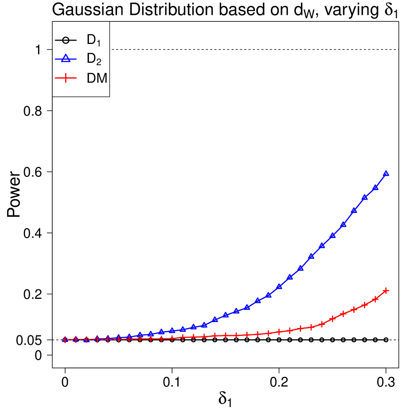
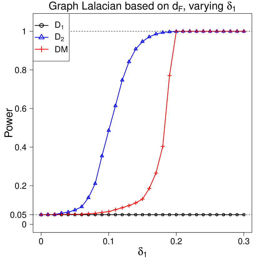
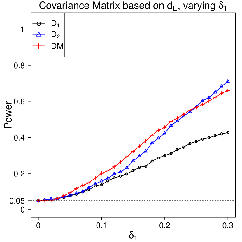
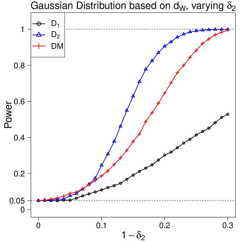
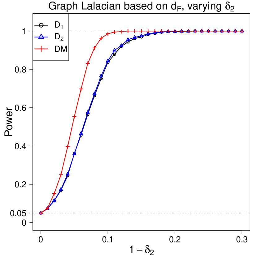
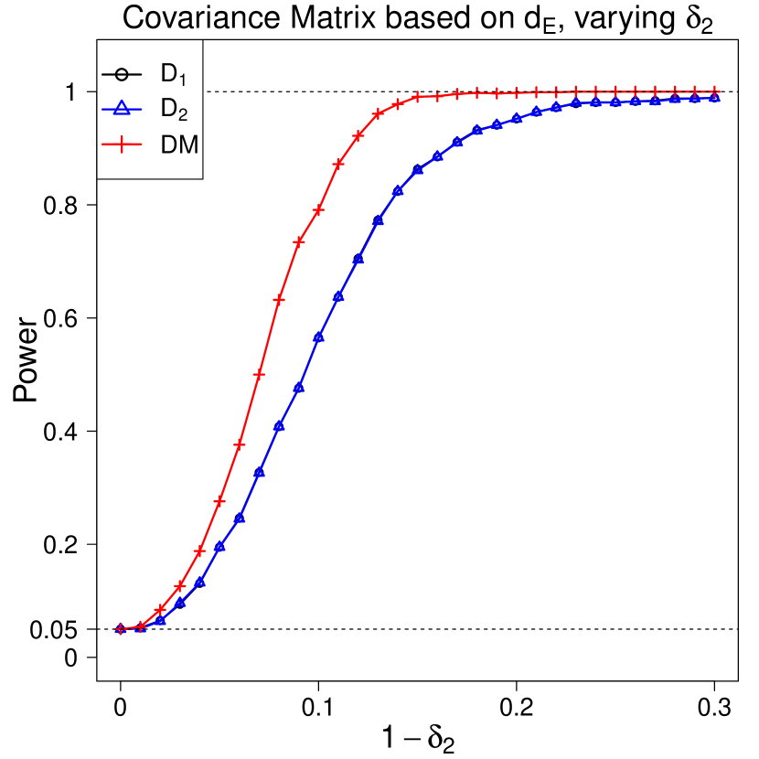
Figure 1: Size-Adjusted Power ($\times 100\%$) at $\alpha=5\%$, Two-Sample Test for all three DGPs, $n_{i}=400$ and $\rho=0.4$

5.2 Change-Point Test

For the change-point testing problems, we set the sample size $n\in\{200,400,800\}$, and trimming parameter as $(\eta_{1},\eta_{2})=(0.15,0.05)$. Table 4 outlines the size performance of our tests and DM test for three DGPs based on 1000 Monte Carlo replications at nominal significance level $\alpha=5\%$. DM tests based asymptotic critical value and bootstraps (with 500 replications) are denoted as $\mathrm{DM}^{a}$ and $\mathrm{DM}^{b}$, respectively.

From Table 4, we find that $SN_{1}$ always exhibits accurate size while $SN_{2}$ is a bit conservative. As a comparison, the tests based on $\mathrm{DM}^{a}$ and $\mathrm{DM}^{b}$ suffer from severe distortion when strong temporal dependence is present, although $\mathrm{DM}^{b}$ is slightly better than $\mathrm{DM}^{a}$ in DGP (i) and (ii).

Table 4: Size Performance ($\times 100\%$) at $\alpha=$5%

			Gaussian Distribution based on $d_{W}$							Graph Laplacian based on $d_{F}$							Covariance Matrix based on $d_{E}$
$\rho$	$n$		$SN_{1}$		$SN_{2}$		$\mathrm{DM}^{a}$	$\mathrm{DM}^{b}$		$SN_{1}$		$SN_{2}$		$\mathrm{DM}^{a}$	$\mathrm{DM}^{b}$		$SN_{1}$		$SN_{2}$		$\mathrm{DM}^{a}$	$\mathrm{DM}^{b}$
-0.4	200		5.5		3.9		15.0	1.9		5.8		3.4		28.9	3.4		6.0		4.6		3.5	5.0
	400		5.5		4.5		13.1	6.7		4.6		1.8		18.9	4.5		5.6		5.1		3.6	5.8
	800		4.4		3.9		13.5	10.3		5.1		3.4		12.3	7.2		4.8		4.4		3.7	5.3
0	200		4.9		2.2		9.2	1.0		5.1		1.6		13.1	1.0		6.2		3.5		3.1	4.1
	400		5.4		2.3		5.7	2.3		5.6		1.7		9.4	2.3		5.3		3.7		4.2	5.8
	800		5.4		3.6		6.1	4.6		5.0		2.6		6.5	3.6		4.7		3.9		3.4	5.7
0.4	200		4.3		3.9		44.7	17.1		5.9		2.4		27.7	3.6		5.4		1.1		7.9	10.1
	400		4.6		2.2		29.8	17.1		6.3		1.9		17.9	4.0		5.2		1.7		6.1	9.2
	800		6.6		2.1		20.4	17.3		5.5		2.1		13.4	6.0		5.3		3.7		6.8	8.3
0.7	200		5.9		10.6		91.4	66.0		5.4		5.8		68.9	20.2		7.9		0.3		29.5	35.3
	400		4.1		5.8		84.5	69.7		5.3		4.0		53.5	22.5		5.9		0.7		22.7	28.9
	800		5.6		3.9		77.8	70.4		4.4		2.3		40.8	25.8		5.5		1.4		20.4	26.1

In Figure 2, we plot the size-adjusted power of our tests and DM test based on bootstrap calibration. Here, the size-adjusted power of DM^b is implemented following Domínguez & Lobato (2000). Similar to the findings in change-point tests, we find that $SN_{1}$ has trivial power in DGP (i) and (ii) when there is only Fréchet mean change and is worst among all three tests. Furthermore, $SN_{2}$ is slightly less powerful compared to DM and the power loss is moderate. Considering its better size control, $SN_{2}$ is preferred.

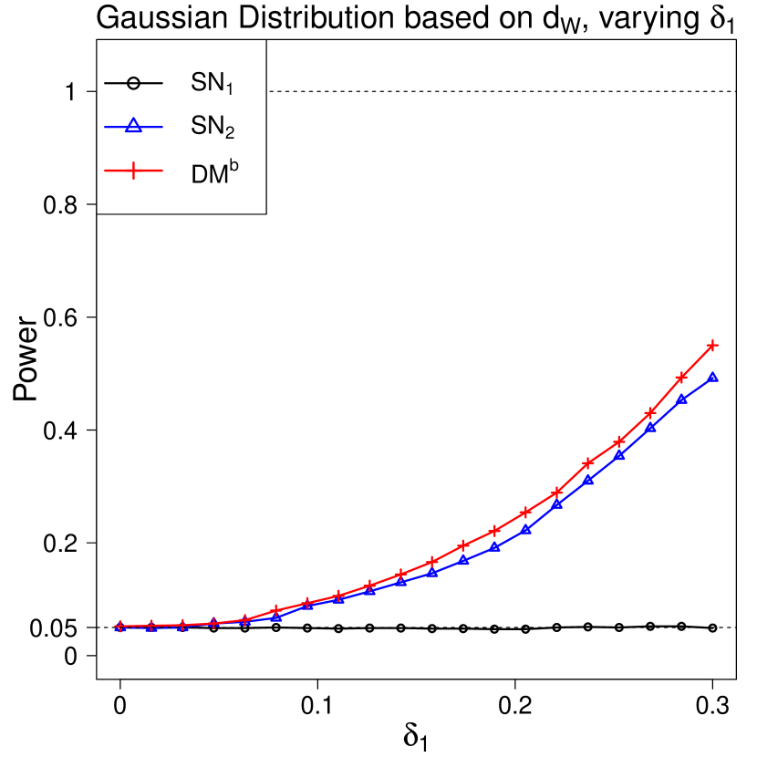
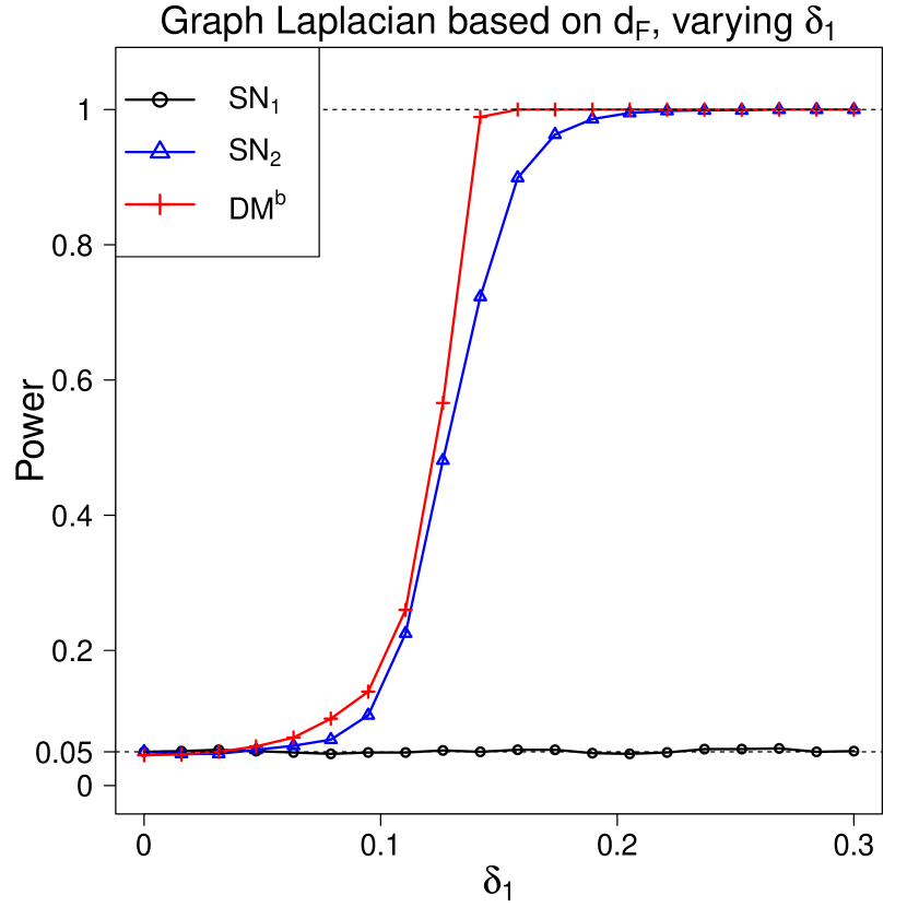
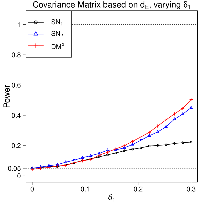
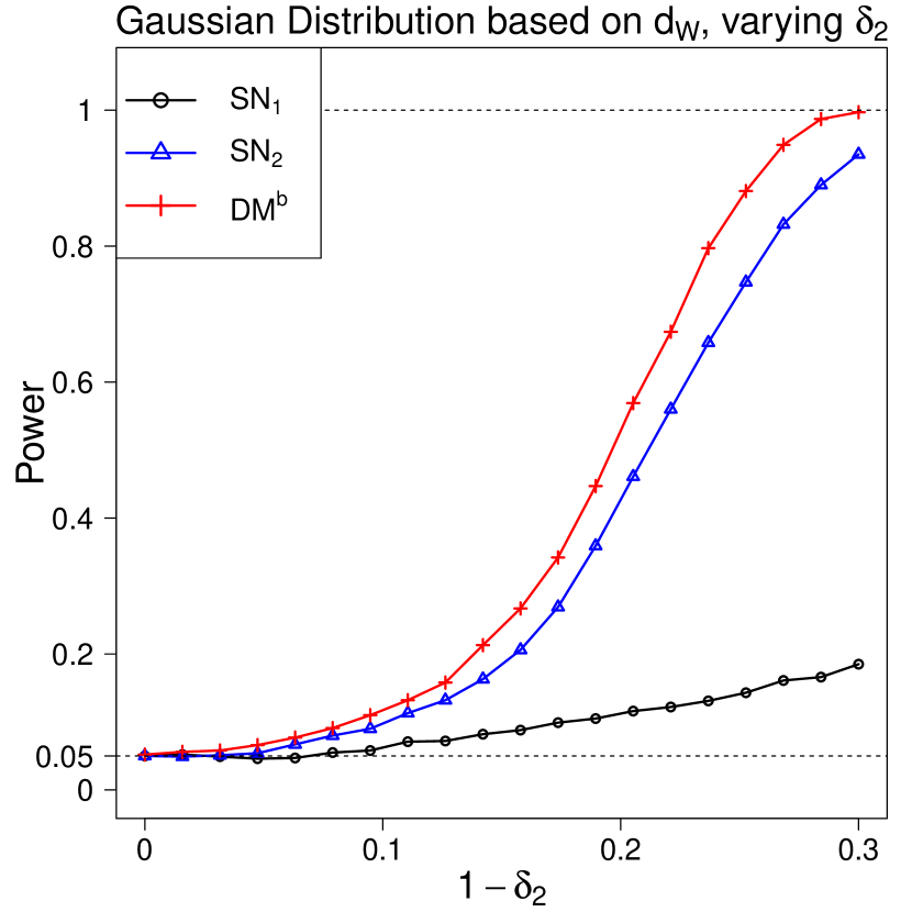
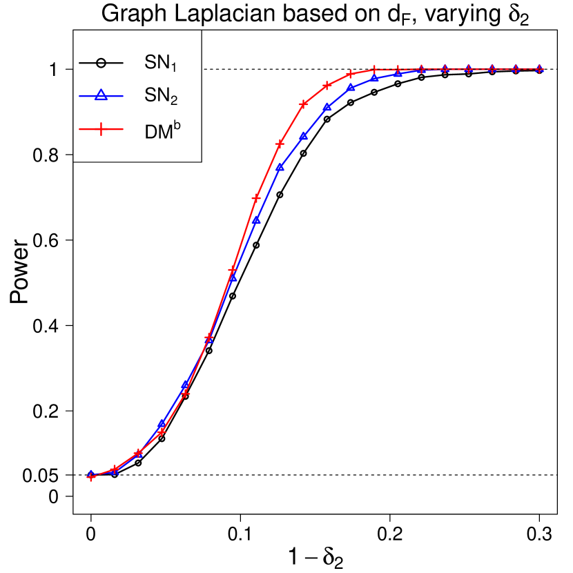
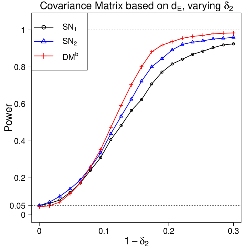
Figure 2: Size-Adjusted Power ($\times 100\%$) at $\alpha=5\%$, Change-Point Test for all three DGPs, $n=400$, $\tau=0.5$, and $\rho=0.4$

We further provide numerical evidence for the estimation accuracy by considering the alternative hypothesis of $\delta_{1}=1-\delta_{2}=0.3$ with true change-point location at $\tau=0.5$ for DGP (i)-(iii) in the main context. When varying sample size $n\in\{400,800,1600\}$, we find that for all DGPs, the histograms of $\hat{\tau}$ (based on SN₂) plotted in Figure 3 get more concentrated around the truth $\tau=0.5$, when sample size increases, which is consistent with our theoretical consistency of $\hat{\tau}$.

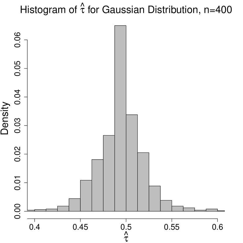
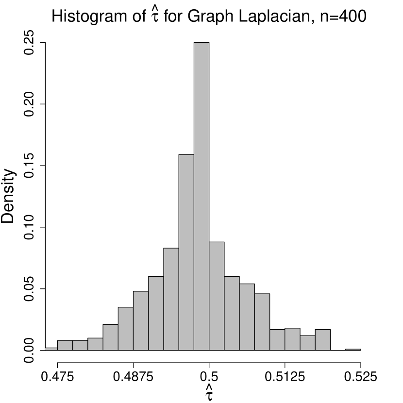
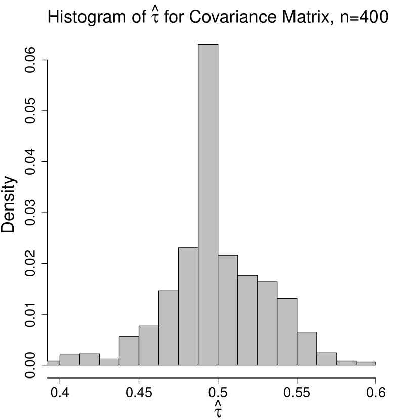
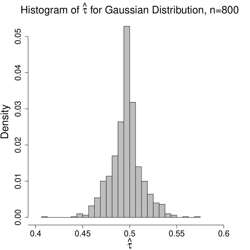
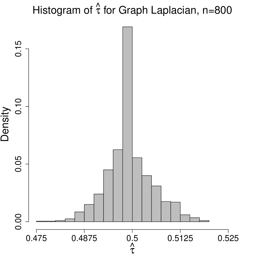
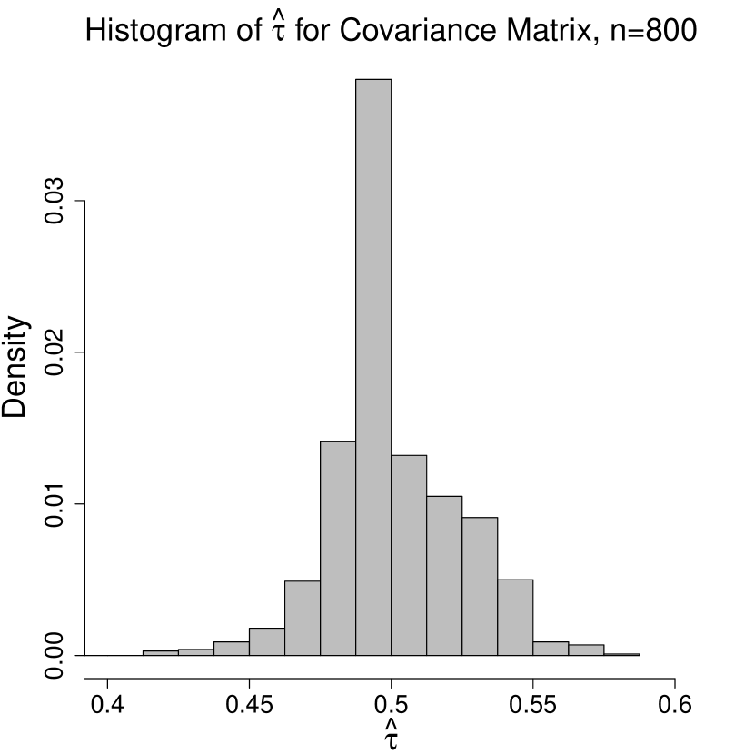
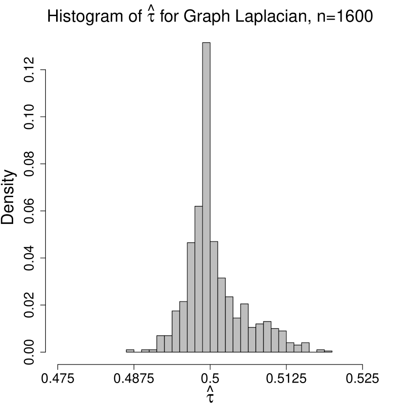
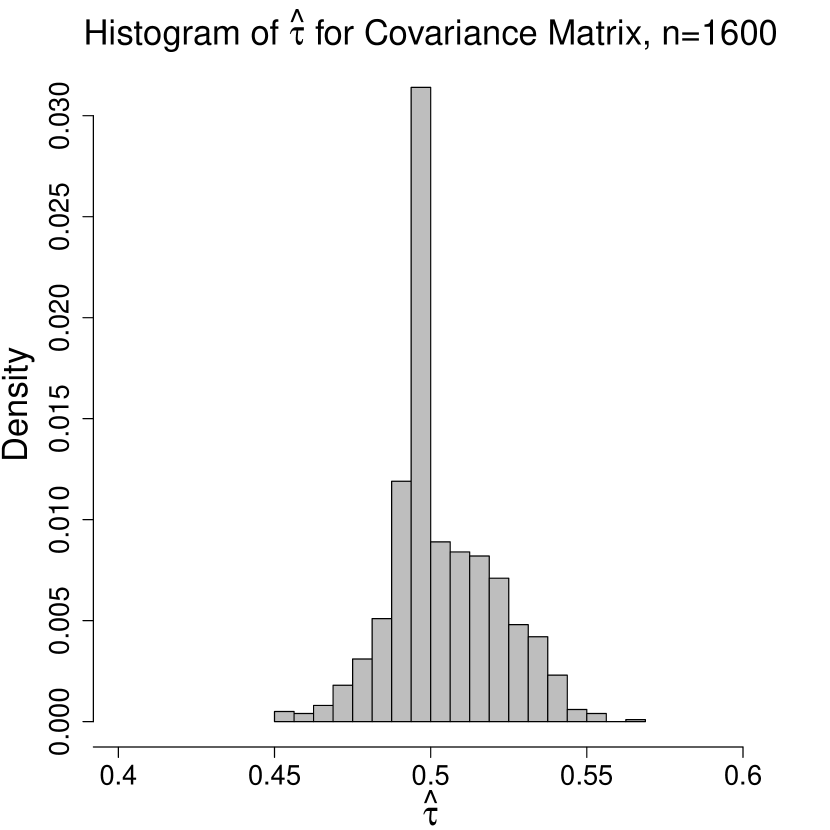
Figure 3: Histogram of Estimated Change-Point Locations for all three DGPs with $\delta_{1}=0.3,\delta_{2}=0.7$, $\tau=0.5$, $\rho=0.4$. Upper: $n=400$. Middle: $n=800$. Lower: $n=1600$.

5.3 Multiple Change Point Detection

For simulations of multiple change point estimation, we consider non-Euclidean time series of length $n=500$ generated from the following two models. These models are the same as before, but reformulated for better presentation purpose.

• Gaussian univariate probability distribution: $Y_{t}=\mathcal{N}(\arctan(U_{t})+\delta_{t,1},$ $\delta_{t,2}^{2}[\arctan(U_{t}^{2})+1]^{2})$.

• covariance matrix: $Y_{t}=(2I_{3}+Z_{t})(2I_{3}+Z_{t})^{\top}$ with $Z_{t}=\delta_{t,1}+\delta_{t,2}\arctan(U_{t}).$

Here, $U_{t}$ are generated according to the AR(1) process $U_{t}=\rho U_{t-1}+\epsilon_{t}$, $\epsilon_{t}\overset{i.i.d.}{\sim}\mathcal{N}(0,1).$ There are 3 change points at $t=110,250$ and $370$. The changes point locations are reflected in the definitions of $\{\delta_{t,1}\}$ and $\{\delta_{t,2}\}$, where

$$\delta_{t,1}=a_{1}\mathbb{I}_{\{n\leq 110\}}+a_{2}\mathbb{I}_{\{110<n\leq 250\}}+a_{3}\mathbb{I}_{\{250<n\leq 370\}}+a_{4}\mathbb{I}_{\{370<n\leq 500\}},$$

$$\delta_{t,2}=b_{1}\mathbb{I}_{\{n\leq 110\}}+b_{2}\mathbb{I}_{\{110<n\leq 250\}}+b_{3}\mathbb{I}_{\{250<n\leq 370\}}+b_{4}\mathbb{I}_{\{370<n\leq 500\}}.$$

For each model, we consider 3 cases that are differentiated by the magnitudes of $a_{i},b_{i},i=1,2,3,4$. For the data generating model of Gaussian distributions, we set

• [Case 1] $(a_{1},a_{2},a_{3},a_{4})=(0,0.7,0,0.8),(b_{1},b_{2},b_{3},b_{4})=(1,1.5,0.7,1.4)$;

• [Case 2] $(a_{1},a_{2},a_{3},a_{4})=(0,0.2,0,0.3),(b_{1},b_{2},b_{3},b_{4})=(0.5,1.5,0.4,1.4)$;

• [Case 3] $(a_{1},a_{2},a_{3},a_{4})=(0,0.5,1.5,3.3),(b_{1},b_{2},b_{3},b_{4})=(0.2,1.5,3.8,6.5)$.

As for the data generating model of covariance matrices, we set

• [Case 1] $(a_{1},a_{2},a_{3},a_{4})=(0,1.2,0,1.3),(b_{1},b_{2},b_{3},b_{4})=(0.8,1.5,0.7,1.6)$;

• [Case 2] $(a_{1},a_{2},a_{3},a_{4})=(0,1,0,1)$, $(b_{1},b_{2},b_{3},b_{4})=(0.5,2,0.4,1.9)$;

• [Case 3] $(a_{1},a_{2},a_{3},a_{4})=(0,2,3.9,5.7)$, $(b_{1},b_{2},b_{3},b_{4})=(0.2,0.7,1.3,2)$.

Cases 1 and 2 correspond to non-monotone changes and Case 3 considers the monotone change. Here, our method described in Section 4.3 is denoted as WBS-$SN_{2}$ (that is, a combination of WBS and our $SN_{2}$ test statistic). The method DM in conjunction with binary segmentation, referred as BS-DM, is proposed in Dubey & Müller (2019) and included in this simulation for comparison purpose. In addition, our statistic $SN_{2}$ in combination with binary segmentation, denoted as BS-$SN_{2}$, is implemented and included as well. The critical values for BS-DM and BS-$SN_{2}$ are obtained from their asymptotic distributions respectively.

The simulation results are shown in Table 5, where we present the ARI (adjusted rand index) and number of detected change points for two dependence levels $\rho=0.3,0.6$. Note that ARI $\in[0,1]$ measures the accuracy of change point estimation and larger ARI corresponds to more accurate estimation. We summarize the main findings as follows. (a) WBS-$SN_{2}$ is the best method in general as it can accommodate both monotonic and non-monotoic changes, and appears quite robust to temporal dependence. For Cases 1 and 2, we see that BS-$SN_{2}$ does not work for non-monotone changes, due to the use of binary segmentation procedure. (b) BS-DM tends to have more false discoveries comparing to the other methods. This is expected, as method DM is primarily proposed for i.i.d data sequence and exhibit serious oversize when there is temporal dependence in Section 5.2. (c) When we increase $\rho=0.3$ to $\rho=0.6$, the performance of WBS-$SN_{2}$ appears quite stable for both distributional time series and covariance matrix time series.

Table 5: Simulation results for multiple change point for sequential Gaussian distributions and covariance matrices based on 200 Monte Carlo repetitions.

Model	Case	$\rho$	Method	# of change points detected						ARI
				$0$	$1$	$2$	$3$	$4$	$\geq 5$
$\begin{array}[]{c}\text{Gaussian}\\ \text{Distribution}\end{array}$	1	0.3	$\text{WBS-}SN_{2}$	$0$	$0$	$0$	$178$	$22$	$0$	$0.971$
			$\text{BS-}SN_{2}$	$200$	$0$	$0$	$0$	$0$	$0$	$0$
			BS-DM	$0$	$0$	$0$	$23$	$15$	$162$	$0.836$
		0.6	$\text{WBS-}SN_{2}$	$0$	$0$	$7$	$116$	$54$	$23$	$0.907$
			$\text{BS-}SN_{2}$	$200$	$0$	$0$	$0$	$0$	$0$	$0$
			BS-DM	$0$	$0$	$0$	$2$	$0$	$198$	$0.516$
	2	0.3	$\text{WBS-}SN_{2}$	$0$	$0$	$0$	$169$	$28$	$3$	$0.980$
			$\text{BS-}SN_{2}$	$200$	$0$	$0$	$0$	$0$	$0$	$0$
			BS-DM	$0$	$0$	$0$	$20$	$14$	$166$	$0.834$
		0.6	$\text{WBS-}SN_{2}$	$0$	$0$	$0$	$101$	$60$	$39$	$0.943$
			$\text{BS-}SN_{2}$	$200$	$0$	$0$	$0$	$0$	$0$	$0$
			BS-DM	$0$	$0$	$0$	$1$	$1$	$198$	$0.526$
	3	0.3	$\text{WBS-}SN_{2}$	$0$	$0$	$0$	$172$	$27$	$1$	$0.981$
			$\text{BS-}SN_{2}$	$0$	$0$	$59$	$82$	$18$	$41$	$0.808$
			BS-DM	$0$	$0$	$0$	$39$	$25$	$136$	$0.893$
		0.6	$\text{WBS-}SN_{2}$	$0$	$0$	$0$	$112$	$65$	$23$	$0.955$
			$\text{BS-}SN_{2}$	$0$	$0$	$45$	$64$	$41$	$50$	$0.828$
			BS-DM	$0$	$0$	$0$	$2$	$4$	$194$	$0.666$
$\begin{array}[]{c}\text{Covariance}\\ \text{Matrix}\end{array}$	1	0.3	$\text{WBS-}SN_{2}$	$0$	$0$	$0$	$200$	$0$	$0$	$0.991$
			$\text{BS-}SN_{2}$	$200$	$0$	$0$	$0$	$0$	$0$	$0$
			BS-DM	$0$	$0$	$0$	$10$	$9$	$181$	$0.807$
		0.6	$\text{WBS-}SN_{2}$	$0$	$0$	$8$	$192$	$0$	$0$	$0.974$
			$\text{BS-}SN_{2}$	$199$	$1$	$0$	$0$	$0$	$0$	$0.002$
			BS-DM	$0$	$0$	$0$	$0$	$0$	$200$	$0.392$
	2	0.3	$\text{WBS-}SN_{2}$	$0$	$0$	$21$	$178$	$1$	$0$	$0.954$
			$\text{BS-}SN_{2}$	$200$	$0$	$0$	$0$	$0$	$0$	$0$
			BS-DM	$6$	$3$	$1$	$4$	$12$	$174$	$0.722$
		0.6	$\text{WBS-}SN_{2}$	$0$	$20$	$82$	$97$	$1$	$0$	$0.800$
			$\text{BS-}SN_{2}$	$200$	$0$	$0$	$0$	$0$	$0$	$0$
			BS-DM	$5$	$0$	$0$	$0$	$0$	$195$	$0.510$
	3	0.3	$\text{WBS-}SN_{2}$	$0$	$0$	$131$	$69$	$0$	$0$	$0.806$
			$\text{BS-}SN_{2}$	$24$	$0$	$124$	$3$	$46$	$3$	$0.468$
			BS-DM	$0$	$0$	$1$	$5$	$10$	$184$	$0.781$
		0.6	$\text{WBS-}SN_{2}$	$0$	$2$	$181$	$16$	$1$	$0$	$0.728$
			$\text{BS-}SN_{2}$	$93$	$1$	$71$	$18$	$17$	$0$	$0.310$
			BS-DM	$0$	$0$	$0$	$0$	$0$	$200$	$0.437$

6 Applications

In this section, we present two real data illustrations, one for two sample testing and the other for change-point detection. Both datasets are in the form of non-Euclidean time series and neither seems to be analyzed before by using techniques that take into account unknown temporal dependence.

6.1 Two sample tests

Mortality data. Here we are interested in comparing the longevity of people living in different countries of Europe. From the Human Mortality Database (https://www.mortality.org/Home/Index), we can obtain a time series that consists of yearly age-at-death distributions for each country. We shall focus on distributions for female from year 1960 to 2015 and there are 26 countries included in the analysis after exclusion of countries with missing data. Pair-wise two sample tests between the included countries are performed using our statistic $D_{2}$ to understand the similarity of age-at-death distributions between different countries. The resulting $p$-value matrix is plotted in Figure 4 (left).

To better present the testing results and gain more insights, we define the dissimilarity between two given countries by subtracting each $p$-value from 1. Treating these dissimilarities as “distances”, we apply multidimensional scaling to “project” each country onto two dimensional plane for visualization. See Figure 4 (right) for the plot of “projected” countries. It appears that several west European countries, including UK, Belgium, Luxembourg, Ireland, and Austria, and Denmark, form a cluster; whereas several central and eastern European countries, including Poland, Latvia, Russian, Bulgaria, Lithuania and Czechia share similar distributions. We suspect the similarity in Mortality distribution is much related to the similarity in their economic development and healthcare system, less dependent on the geographical locations.

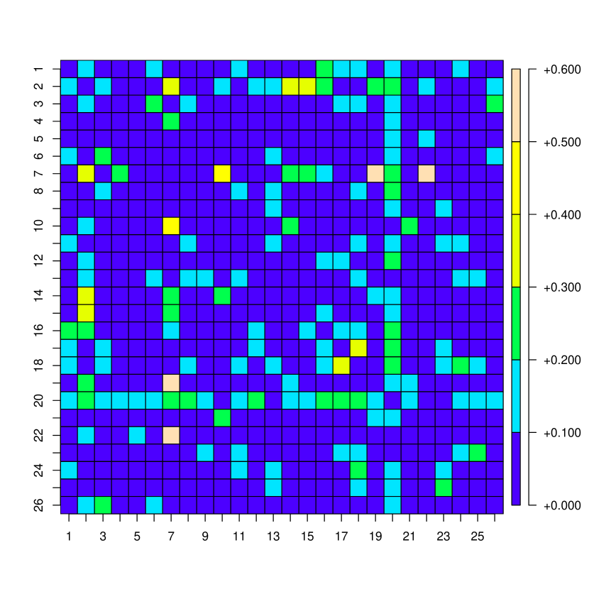
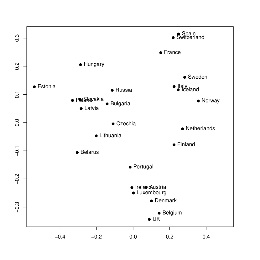
Figure 4: Application to Mortality data. The left figure is the plot of $p$-value matrix, where the 26 countries, Austria, Belarus, Belgium, Bulgaria, Czechia, Denmark, Estonia, Finland, France, Hungary, Iceland, Ireland, Italy, Latvia, Lithuania, Luxembourg, Netherlands, Norway, Poland, Portugal, Russia, Slovakia, Spain, Sweden, Switzerland, UK, are labeled by $1,2,\dots,26$ respectively. The right figure is the plot of points from multidimensional scaling with dissimilarity between any countries defined as subtracting the corresponding $p$-value from 1.

6.2 Change point detection

Cryptocurrency data. Detecting change points in the Pearson correlation matrices for a set of interested cryptocurrencies can uncover structural breaks in the correlation of these cryptocurrencies and can play an important role in the investors’ investment decisions. Here, we construct the daily Pearson correlation matrices from minute prices of Bitcoin, Doge coin, Cardano, Monero and Chainlink for year 2021. The cryptocurrency data can be downloaded at https://www.cryptodatadownload.com/analytics/correlation-heatmap/. See Figure 5 for the plot of time series of pairwise correlations. Three methods, namely, our $SN_{2}$ test combined with WBS (WBS-$SN_{2}$), $SN_{2}$ test combined with binary segmentation (BS-$SN_{2}$), and DM test of Dubey & Müller (2019) in conjunction with binary segmentation (BS-DM), are applied to detect potential change points for this time series,

Method WBS-$SN_{2}$ detects an abrupt change on day 2021-05-17 and method BS-$SN_{2}$ detects a change point on day 2021-04-29. By comparison, more than 10 change points are detected by BS-DM and we suspect that many of them are false discoveries (see Section 5.3 for simulation evidence of BS-DM’s tendency of over-detection). The change point in mid-May 2021 is well expected and corresponds to a major crush in crypto market that wiped out 1 trillion dollars. The major causes of this crush are the withdrawal of Tesla’s commitment to accept Bitcoin as payment and warnings regarding cryptocurrency sent by Chinese central bank to the financial institutes and business in China. Since this major crush, the market has been dominated by negative sentiments and fear for a recession. We refer the following CNN article for some discussions about this crush https://www.cnn.com/2021/05/22/investing/crypto-crash-bitcoin-regulation/index.html.

Figure 5: Plot of time series of pairwise correlations. Red vertical line indicates detected change point by WBS-$SN_{2}$.

7 Conclusion

Motivated by increasing availability of non-Euclidean time series data, this paper considers two-sample testing and change-point detection for temporally dependent random objects. Our inferential framework builds upon the nascent SN technique, which has been mainly developed for conventional Euclidean time series or functional time series in Hilbert space, and the extension of SN to the time series of objects residing in metric spaces is the first in the literature. The proposed tests are robust to weak temporal dependence, enjoy effortless tuning and are broadly applicable to many non-Euclidean data types with easily verified technical conditions. On the theory front, we derive the asymptotic distributions of our two sample and change-point tests under both null and local alternatives of order $O(n^{-1/2})$. Furthermore, for change-point problem, the consistency of the change-point estimator is established under mild conditions. Both simulation and real data illustrations demonstrate the robustness of our test with respect to temporal dependence and the effectiveness in testing and estimation problems.

To conclude, we mention several interesting but unsolved problems for analyzing non-Euclidean time series. For example, although powerful against Fréchet mean differences/changes, the testing statistics developed in this paper rely on the asymptotic behaviors of Fréchet (sub)sample variances. It is imperative to construct formal tests that can target directly at Fréchet mean differences/changes. For the change-point detection problem in non-Euclidean data, the existing literature, including this paper, only derives the consistency of the change-point estimator. It would be very useful to derive explicit convergence rate and the asymptotic distribution of the change-point estimator, which is needed for confidence interval construction. Also it would be interesting to study how to detect structural changes when the underlying distributions of random objects change smoothly. We leave these topics for future investigation.

Appendix A Technical Proofs

A.1 Auxiliary Lemmas

We first introduce some notations. We denote $o_{up}(\cdot)$ as the uniform $o_{p}(\cdot)$ w.r.t. the partial sum index $(a,b)\in\mathcal{I}_{\eta}$. Let $M_{n}(\omega,[a,b])=n^{-1}\sum_{t=\lfloor na\rfloor+1}^{\lfloor nb\rfloor}f_{\omega}(Y_{t})$, where $f_{\omega}(Y)=d^{2}(Y,\omega)-d^{2}(Y,\mu)$, then it is clear that

$$\hat{\mu}_{[a,b]}=\arg\min_{\omega\in\Omega}M_{n}(\omega,[a,b]).$$

Let $\tilde{V}_{[a,b]}=\frac{1}{\lfloor nb\rfloor-\lfloor na\rfloor}\sum_{t=\lfloor na\rfloor+1}^{\lfloor nb\rfloor}d^{2}\left(Y_{t},\mu\right)$.

The following three main lemmas are verified under Assumption 2.1-2.5, and they are used repeatedly throughout the proof for main theorems.

Lemma A.1.

$\sup_{(a,b)\in\mathcal{I}_{\eta}}\sqrt{n}d(\hat{\mu}_{[a,b]},\mu)=O_{p}(1)$.

Proof.

(1). We first show the uniform convergence, i.e. $\sup_{(a,b)\in\mathcal{I}_{\eta}}d(\hat{\mu}_{[a,b]},\mu)=o_{up}(1).$

For any $\epsilon>0$, define

$$\psi(\epsilon):=\inf_{d(\omega,\mu)>\epsilon}\mathbb{E}f_{\omega}(Y),$$ (8)

and we know by that $\psi(\epsilon)>0$ by the uniqueness of $\mu$ in Assumption 2.1.

Hence, let $M(\omega,[a,b])=(b-a)\mathbb{E}f_{\omega}(Y)$, we have

$$P\Bigg{(}\sup_{(a,b)\in\mathcal{I}_{\eta}}d(\hat{\mu}_{[a,b]},\mu)>\epsilon\Bigg{)}$$

$$= {P\Bigg{(}\bigcup_{(a,b)\in\mathcal{I}_{\eta}}\left\{d(\hat{\mu}_{[a,b]},\mu)>\epsilon\right\}\Bigg{)}}$$

$$\leq P\Bigg{(}\bigcup_{(a,b)\in\mathcal{I}_{\eta}}\left\{M(\hat{\mu}_{[a,b]},[a,b])-\inf_{d(\omega,\mu)>\epsilon}M(\omega,[a,b])\geq 0\right\}\Bigg{)}$$

$$\leq P\Bigg{(}\bigcup_{(a,b)\in\mathcal{I}_{\eta}}\left\{M(\hat{\mu}_{[a,b]},[a,b])\geq\eta\psi(\epsilon)/2\right\}\Bigg{)}$$

$$\leq P\Bigg{(}\bigcup_{(a,b)\in\mathcal{I}_{\eta}}\Bigg{\{}M(\hat{\mu}_{[a,b]},[a,b])-M_{n}(\hat{\mu}_{[a,b]},[a,b])$$

$$\hskip 113.81102pt+M_{n}(\mu,[a,b])-M(\mu,[a,b])\geq\eta\psi(\epsilon)/2\Bigg{\}}\Bigg{)}$$

$$\leq P\Bigg{(}\sup_{(a,b)\in\mathcal{I}_{\eta}}\sup_{\omega\in\Omega}\left|M_{n}(\omega,[a,b])-M(\omega,[a,b])\right|\geq\eta\psi(\epsilon)/4\Bigg{)}$$

where the first inequality holds because the event $\{d(\hat{\mu}_{[a,b]},\mu)>\epsilon\}$ implies that $\hat{\mu}_{[a,b]}\in\{\omega\in\Omega:d(\omega,\mu)>\epsilon\}$, and thus $M(\hat{\mu}_{[a,b]},[a,b])\geq\inf_{d(\omega,\mu)>\epsilon}M(\omega,[a,b])$; the second inequality holds by $b-a\geq\eta$ (hence $({\lfloor nb\rfloor-\lfloor na\rfloor})/{n}>\eta/2$ for large $n$) and the definition of (8) such that $\inf_{d(\omega,\mu)>\epsilon}M(\omega,[a,b])=(b-a)\psi(\epsilon)>\eta\psi(\epsilon)/2$; and the third holds by that $M(\mu,[a,b])=0$ and $M_{n}(\mu,[a,b])\geq M_{n}(\hat{\mu}_{[a,b]},[a,b])$.

Note $M_{n}(\omega,[a,b])-M(\omega,[a,b])=M_{n}(\omega,[0,b])-M(\omega,[0,b])-M_{n}(\omega,[0,a])+M(\omega,[0,a])$. Therefore, it suffices to show the weak convergence of the process $\{M_{n}(\omega,[0,u])-M(\omega,[0,u]),u\in[0,1],\omega\in\Omega\}$ to zero. Note the pointwise convergence holds easily by the boundedness of $f_{\omega}$ and Assumption 2.3, so we only need to show the stochastic equicontinuity, i.e.

$$\limsup_{n\to\infty}P\Bigg{(}\sup_{|u-v|<\delta_{1},d(\omega_{1},\omega_{2})<\delta_{2}}|M_{n}(\omega_{1},[0,u])-M(\omega_{1},[0,u])$$

$$\hskip 113.81102pt-M_{n}(\omega_{2},[0,v])+M(\omega_{2},[0,v])|>\epsilon\Bigg{)}\to 0$$

as $\max(\delta_{1},\delta_{2})\to 0$.

Then, by triangle inequality, we have

$$|M_{n}(\omega_{1},[0,u])-M(\omega_{1},[0,u])-M_{n}(\omega_{2},[0,v])+M(\omega_{2},[0,v])|$$

$$\leq |M_{n}(\omega_{1},[0,u])-M_{n}(\omega_{1},[0,v])|+|M_{n}(\omega_{1},[0,v])-M_{n}(\omega_{2},[0,v])|$$

$$+|M(\omega_{1},[0,u])-M(\omega_{1},[0,v])|+|M(\omega_{1},[0,v])-M(\omega_{2},[0,v])|$$

$$:= \sum_{i=1}^{4}R_{n,i}.$$

Without loss of generality, we assume $v>u$, and by the boundedness of the metric, we have for some $K>0$,

$$R_{n,1}\leq n^{-1}\sum_{t=\lfloor nu\rfloor+1}^{\lfloor nv\rfloor}d^{2}(Y_{t},\omega_{1})\leq K|u-v|\leq K\delta_{1}.$$

Similarly, $R_{n,3}\leq K$. Furthermore, we can see that $R_{n,2},R_{n,4}\leq 2\mathrm{diam}(\Omega)d(\omega_{1},\omega_{2})\leq K\delta_{2}.$ Hence, the result follows by letting $\delta_{1}$ and $\delta_{2}$ sufficiently small.

Thus, the uniform convergence holds.

(2). We then derive the convergence rate based on Assumption 2.5.

By the consistency, we have for any $\delta>0$, $P(\sup_{(a,b)\in\mathcal{I}_{\eta}}d(\hat{\mu}_{[a,b]},\mu)\leq\delta)\to 1$. Hence, on the event that $\sup_{(a,b)\in\mathcal{I}_{\eta}}d(\hat{\mu}_{a,b},\mu)\leq\delta$, and note that $M_{n}(\mu,[a,b])=n^{-1}\sum_{t=\lfloor na\rfloor+1}^{\lfloor nb\rfloor}[d^{2}(Y_{t},\mu)-d^{2}(Y_{t},\mu)]=0$, we have

$$0= M_{n}(\mu,[a,b])$$

$$\geq M_{n}(\hat{\mu}_{[a,b]},[a,b])$$

$$= K_{d}\frac{\lfloor nb\rfloor-\lfloor na\rfloor}{n}d^{2}(\hat{\mu}_{[a,b]},\mu)+n^{-1}\sum_{t=\lfloor na\rfloor+1}^{\lfloor nb\rfloor}\left[g(Y_{t},\hat{\mu}_{[a,b]},\mu)+R(Y_{t},\hat{\mu}_{[a,b]},\mu)\right]$$

$$\geq \frac{K_{d}\eta}{2}d^{2}(\hat{\mu}_{[a,b]},\mu)$$

$$\hskip 14.22636pt+d(\hat{\mu}_{[a,b]},\mu)\left[\frac{n^{-1}\sum_{t=\lfloor na\rfloor+1}^{\lfloor nb\rfloor}g(Y_{t},\hat{\mu}_{[a,b]},\mu)}{d(\hat{\mu}_{[a,b]},\mu)}+o_{up}(n^{-1/2}+d(\hat{\mu}_{[a,b]},\mu))\right],$$

where the last inequality holds by Assumption 2.5 and the fact $({\lfloor nb\rfloor-\lfloor na\rfloor})/{n}>\eta/2$ for large $n$.

Note the above analysis holds uniformly for $(a,b)\in\mathcal{I}_{\eta}$, this implies that

$$\sup_{(a,b)\in\mathcal{I}_{\eta}}\left[\frac{K_{d}\eta}{2}d(\hat{\mu}_{[a,b]},\mu)-o_{up}(d(\hat{\mu}_{[a,b]},\mu))\right]$$

$$\leq n^{-1/2}\sup_{(a,b)\in\mathcal{I}_{\eta}}\left|\frac{n^{-1/2}\sum_{t=\lfloor na\rfloor+1}^{\lfloor nb\rfloor}g(Y_{t},\hat{\mu}_{[a,b]},\mu)}{d(\hat{\mu}_{[a,b]},\mu)}\right|+o_{up}(n^{-1/2})=O_{p}(n^{-1/2}),$$

and hence $\sup_{(a,b)\in\mathcal{I}_{\eta}}d(\hat{\mu}_{[a,b]},\mu)=O_{p}(n^{-1/2})$. ∎

Lemma A.2.

$\sup_{(a,b)\in\mathcal{I}_{\eta}}\sqrt{n}|\hat{V}_{[a,b]}-\tilde{V}_{[a,b]}|=o_{p}(1)$.

Proof.

By Lemma A.1, and Assumption 2.5, we have

$$\sup_{(a,b)\in\mathcal{I}_{\eta}}\sqrt{n}M_{n}(\hat{\mu}_{[a,b]},[a,b])$$

$$\leq K_{d}\sup_{(a,b)\in\mathcal{I}_{\eta}}d(\hat{\mu}_{[a,b]},\mu)\sup_{(a,b)\in\mathcal{I}_{\eta}}\Bigg{|}\sqrt{n}d(\hat{\mu}_{[a,b]},\mu)$$

$$\hskip 28.45274pt+\frac{n^{-1/2}\sum_{t=\lfloor na\rfloor+1}^{\lfloor nb\rfloor}g(Y_{t},\hat{\mu}_{[a,b]},\mu)}{d(\hat{\mu}_{[a,b]},\mu)}+o_{up}(1+\sqrt{n}d(\hat{\mu}_{[a,b]},\mu))\Bigg{|}$$

$$= O_{p}(n^{-1/2}).$$

Hence, we have that

$$\sup_{(a,b)\in\mathcal{I}_{\eta}}\sqrt{n}|\hat{V}_{[a,b]}-\tilde{V}_{[a,b]}|\leq\eta^{-1}\sup_{(a,b)\in\mathcal{I}_{\eta}}\sqrt{n}M_{n}(\hat{\mu}_{[a,b]},[a,b]),$$

the result follows. ∎

Lemma A.3.

Let $\hat{V}^{C}_{[a,b]}(\tilde{\omega})=\frac{1}{\lfloor nb\rfloor-\lfloor na\rfloor}\sum_{t=\lfloor na\rfloor+1}^{\lfloor nb\rfloor}d^{2}(Y_{i},\tilde{\omega}),$ where $\tilde{\omega}\in\Omega$ is a random object such that

$$\sqrt{n}\sup_{(a,b)\in\mathcal{I}_{\eta}}d(\tilde{\omega},\hat{\mu}_{[a,b]})=O_{p}(1).$$

Then,

$$\sqrt{n}\sup_{(a,b)\in\mathcal{I}_{\eta}}|\hat{V}^{C}_{[a,b]}(\tilde{\omega})-\tilde{V}_{[a,b]}|=o_{p}(1).$$

Proof.

By triangle inequality and Lemma A.2,

$$\sqrt{n}\sup_{(a,b)\in\mathcal{I}_{\eta}}|\hat{V}^{C}_{[a,b]}(\tilde{\omega})-\tilde{V}_{[a,b]}|$$

$$= \sup_{(a,b)\in\mathcal{I}_{\eta}}\left|\frac{\sqrt{n}}{\lfloor nb\rfloor-\lfloor na\rfloor}\sum_{t=\lfloor na\rfloor+1}^{\lfloor nb\rfloor}d^{2}\left(Y_{t},\tilde{\omega}\right)-d^{2}(Y_{i},\mu)\right|$$

$$\leq (\eta/2)^{-1}\sup_{(a,b)\in\mathcal{I}_{\eta}}\sqrt{n}M_{n}(\tilde{\omega},[a,b]).$$

Note by triangle inequality for the metric, $d(\tilde{\omega},\mu)\leq d(\hat{\mu}_{[a,b]},\mu)+d(\tilde{\omega},\hat{\mu}_{[a,b]})=O_{p}(n^{-1/2})$, and we know that $d(\tilde{\omega},\mu)<\delta$ with probability tending to 1, and on this event, by Assumption 2.5,

$$\sqrt{n}M_{n}(\tilde{\omega},[a,b])\leq K_{d}d^{2}(\tilde{\omega},\mu)+n^{-1}\left|\sum_{t=\lfloor na\rfloor+1}^{\lfloor nb\rfloor}g(Y_{t},\tilde{\omega},\mu)\right|$$

$$\hskip 28.45274pt+n^{-1}\left|\sum_{t=\lfloor na\rfloor+1}^{\lfloor nb\rfloor}R(Y_{t},\tilde{\omega},\mu)\right|.$$

Similar to the proof of Lemma A.2, we get the result. ∎

A.2 Proof of Theorems in Section 3

Let $\tilde{V}^{(1)}_{r}=\frac{1}{\lfloor rn_{1}\rfloor}\sum_{t=1}^{\lfloor rn_{1}\rfloor}d^{2}(Y_{t}^{(1)},\mu^{(1)})$, and $\tilde{V}^{(2)}_{r}=\frac{1}{\lfloor rn_{2}\rfloor}\sum_{t=1}^{\lfloor rn_{2}\rfloor}d^{2}(Y_{t}^{(2)},\mu^{(2)})$.

For each $r\in[\eta,1]$, we consider the decomposition,

$$\begin{split}\sqrt{n}T_{n}(r)=&{\sqrt{n}}r(\hat{V}^{(1)}_{r}-\hat{V}^{(2)}_{r})\\ =&{\sqrt{n}}r(\hat{V}^{(1)}_{r}-\tilde{V}^{(1)}_{r}+\tilde{V}^{(1)}_{r}-V^{(1)})\\ &-{\sqrt{n}}r(\hat{V}^{(2)}_{r}-\tilde{V}^{(2)}_{r}+\tilde{V}^{(2)}_{r}-V^{(2)})\\ &+{\sqrt{n}}r(V^{(1)}-V^{(2)})\\ :=&R_{n,1}(r)+R_{n,2}(r)+R_{n,3}(r).\end{split}$$ (9)

and

$$\begin{split}\sqrt{n}T_{n}^{C}(r)=&\sqrt{n}r(\hat{V}^{C,(1)}_{r}-\tilde{V}^{(1)}_{r})-\sqrt{n}r(\hat{V}^{(1)}_{r}-\tilde{V}^{(1)}_{r})\\ &+\sqrt{n}r(\hat{V}^{C,(2)}_{r}-\tilde{V}^{(2)}_{r})-\sqrt{n}r(\hat{V}^{(2)}_{r}-\tilde{V}^{(2)}_{r})\\ :=&R^{C}_{n,1}(r)+R^{C}_{n,2}(r)+R^{C}_{n,3}(r)+R^{C}_{n,4}(r).\end{split}$$ (10)

By Lemma A.2,

$$\sup_{r\in[\eta,1]}\sqrt{n}r(\hat{V}^{(1)}_{r}-\tilde{V}^{(1)}_{r})=o_{p}(1),\quad\sup_{r\in[\eta,1]}\sqrt{n}r(\hat{V}^{(2)}_{r}-\tilde{V}^{(2)}_{r})=o_{p}(1),$$ (11)

i.e.

$$\left\{R^{C}_{n,2}(r)+R^{C}_{n,4}(r)\right\}_{r\in[\eta,1]}\Rightarrow 0.$$ (12)

Furthermore, by Assumption 3.1,

$$\sqrt{n}r(\hat{V}^{(1)}_{r}-V^{(1)})\Rightarrow\gamma_{1}^{-1}\sigma_{1}B^{(1)}(\gamma_{1}r),\quad\sqrt{n}r(\hat{V}^{(2)}_{r}-V^{(2)})\Rightarrow\gamma_{2}^{-1}\sigma_{2}B^{(2)}(\gamma_{2}r).$$

This implies that

$$\left\{R_{n,1}(r)+R_{n,2}(r)\right\}_{r\in[\eta,1]}\Rightarrow\{\xi_{\gamma_{1},\gamma_{2}}(r;\sigma_{1},\sigma_{2})\}_{r\in[\eta,1]}.$$ (13)

Proof of Theorem 3.1

Under $\mathbb{H}_{0}$, $R_{n,3}(r)\equiv 0$, and $\mu^{(1)}=\mu^{(2)}=\mu$. Hence, by (9) and (13), we obtain that

$$\{\sqrt{n}T_{n}(r)\}_{r\in[\eta,1]}\Rightarrow\{\xi_{\gamma_{1},\gamma_{2}}(r;\sigma_{1},\sigma_{2})\}_{r\in[\eta,1]}.$$

Next, by Lemma A.1, can obtain that

$$\sqrt{n}\sup_{r\in[\eta,1]}d(\hat{\mu}^{(1)}_{r},\mu)=o_{p}(1),\quad\sqrt{n}\sup_{r\in[\eta,1]}d(\hat{\mu}^{(2)}_{r},\mu)=o_{p}(1).$$

Hence, by Lemma A.3, we have

$$\left\{R^{C}_{n,1}(r)+R^{C}_{n,3}(r)\right\}_{r\in[\eta,1]}\Rightarrow 0.$$

Together with (12), we have

$$\{\sqrt{n}T^{C}_{n}(r)\}_{r\in[\eta,1]}\Rightarrow 0.$$

Hence, by continuous mapping theorem, for both $i=1,2$,

$$D_{n,i}\to_{d}\frac{\xi^{2}_{\gamma_{1},\gamma_{2}}(1;\sigma_{1},\sigma_{2})}{\int_{\eta}^{1}\left[\xi_{\gamma_{1},\gamma_{2}}(r;\sigma_{1},\sigma_{2})-r\xi_{\gamma_{1},\gamma_{2}}(1;\sigma_{1},\sigma_{2})\right]^{2}dr}.$$

∎

Proof of Theorem 3.2

In view of (9) and (13),

$$\left\{\sqrt{n}T_{n}(r)\right\}_{r\in[\eta,1]}\Rightarrow\left\{\xi_{\gamma_{1},\gamma_{2}}(r;\sigma_{1},\sigma_{2})+rn^{-\kappa_{V}+1/2}\Delta_{V}\right\}_{r\in[\eta,1]}.$$

Hence

• For $\kappa_{V}\in(1/2,\infty)$, $\left\{\sqrt{n}T_{n}(r)\right\}\Rightarrow\left\{\xi_{\gamma_{1},\gamma_{2}}(r;\sigma_{1},\sigma_{2})\right\}_{r\in[\eta,1]}.$

• For $\kappa_{V}=1/2$, $\left\{\sqrt{n}T_{n}(r)\right\}_{r\in[\eta,1]}\Rightarrow\left\{\xi_{\gamma_{1},\gamma_{2}}(r;\sigma_{1},\sigma_{2})+r\Delta_{V}\right\}_{r\in[\eta,1]}.$

• For $\kappa_{V}\in(0,1/2)$, $\sqrt{n}T_{n}(1)\to_{p}\infty$, and $\left\{\sqrt{n}T_{n}(r)-\sqrt{n}rT_{n}(1)\right\}_{r\in[\eta,1]}\Rightarrow\left\{\xi_{\gamma_{1},\gamma_{2}}(r;\sigma_{1},\sigma_{2})-r\xi_{\gamma_{1},\gamma_{2}}(1;\sigma_{1},\sigma_{2})\right\}_{r\in[\eta,1]}$.

Next, we focus on $\sqrt{n}T_{n}^{C}(r)$. When $\kappa_{M}\in(0,\infty)$, it holds that $d(\mu^{(1)},\mu^{(2)})=O(n^{-\kappa_{M}/2})=o(1)$, and by triangle inequality, for any $r\in[\eta,1]$,

$$|d(\mu^{(1)},\mu^{(2)})-d(\hat{\mu}^{(2)}_{r},\mu^{(2)})|\leq d(\hat{\mu}^{(2)}_{r},\mu^{(1)})\leq|d(\mu^{(1)},\mu^{(2)})+d(\hat{\mu}^{(2)}_{r},\mu^{(2)})|.$$ (14)

By Lemma A.1, we have $\sup_{r\in[\eta,1]}d(\hat{\mu}^{(2)}_{r},\mu^{(2)})=O_{p}(n^{-1/2})$. This and (14) imply that

• when $\kappa_{M}\in(1/2,\infty)$, $d^{2}(\hat{\mu}^{(2)}_{r},\mu^{(1)})=o_{up}(n^{-1/2})$;

• when $\kappa_{M}\in(0,1/2]$, $d^{2}(\hat{\mu}^{(2)}_{r},\mu^{(1)})=d^{2}(\mu^{(1)},\mu^{(2)})+o_{up}(n^{-1/2})=n^{-\kappa_{M}}\Delta_{M}+o_{up}(n^{-1/2})$.

Similarly,

• when $\kappa_{M}\in(1/2,\infty)$, $d^{2}(\hat{\mu}^{(1)}_{r},\mu^{(2)})=o_{up}(n^{-1/2})$;

• when $\kappa_{M}\in(0,1/2]$, $d^{2}(\hat{\mu}^{(1)}_{r},\mu^{(2)})=n^{-\kappa_{M}}\Delta_{M}+o_{up}(n^{-1/2})$.

Furthermore, by Assumption 2.5, equations (10) and (12), we obtain

$$\begin{split}&\sqrt{n}T_{n}^{C}(r)=R_{n,1}^{C}(r)+R_{n,3}^{C}(r)+o_{up}(1)\\ =&\sqrt{n}K_{d}rd^{2}(\hat{\mu}^{(2)}_{r},\mu^{(1)})+rd(\hat{\mu}^{(2)}_{r},\mu^{(1)})\left[\frac{n^{-1/2}\sum_{t=1}^{\lfloor\gamma_{1}nr\rfloor}g(Y_{t}^{(1)},\hat{\mu}^{(2)}_{r},\mu^{(1)})}{d(\hat{\mu}^{(2)}_{r},\mu^{(1)})}\right]\\ &\hskip 28.45274pt+o_{up}(d(\hat{\mu}^{(2)}_{r},\mu^{(1)})+\sqrt{n}d^{2}(\hat{\mu}^{(2)}_{r},\mu^{(1)}))\\ &+\sqrt{n}K_{d}rd^{2}(\hat{\mu}^{(1)}_{r},\mu^{(2)})+rd(\hat{\mu}^{(1)}_{r},\mu^{(2)})\left[\frac{n^{-1/2}\sum_{t=1}^{\lfloor\gamma_{2}nr\rfloor}g(Y_{t}^{(2)},\hat{\mu}^{(1)}_{r},\mu^{(2)})}{d(\hat{\mu}^{(1)}_{r},\mu^{(2)})}\right]\\ &\hskip 28.45274pt+o_{up}(d(\hat{\mu}^{(1)}_{r},\mu^{(2)})+\sqrt{n}d^{2}(\hat{\mu}^{(1)}_{r},\mu^{(2)}))\\ &+o_{up}(1).\end{split}$$ (15)

• For $\kappa_{M}\in(1/2,\infty)$, $d^{2}(\hat{\mu}^{(2)}_{r},\mu^{(1)})=o_{up}(n^{-1/2}),$ and $d^{2}(\hat{\mu}^{(1)}_{r},\mu^{(2)})=o_{up}(n^{-1/2}).$ Hence, $\{\sqrt{n}T_{n}^{C}(r)\}_{r\in[\eta,1]}\Rightarrow 0$.

• For $\kappa_{M}=1/2$, we note that $d^{2}(\hat{\mu}^{(2)}_{r},\mu^{(1)})=n^{-1/2}\Delta_{M}+o_{up}(1),$ and $d^{2}(\hat{\mu}^{(1)}_{n},\mu^{(2)})=n^{-1/2}\Delta_{M}+o_{up}(1).$ Hence, $\{\sqrt{n}T_{n}^{C}(r)\}_{r\in[\eta,1]}\Rightarrow\{2rK_{d}\Delta_{M}\}_{r\in[\eta,1]}$, and $\{\sqrt{n}[T_{n}^{C}(r)-rT_{n}^{C}(1)]\}_{r\in[\eta,1]}\Rightarrow 0$.

• For $\kappa_{M}\in(0,1/2)$, we multiply $n^{2\kappa_{M}-1}$ on both denominator and numerator of $D_{n,2}$, and obtain

  $$D_{n,2}=\frac{n^{2\kappa_{M}}\left\{\left[T_{n}(1)\right]^{2}+\left[T_{n}^{C}(1)\right]^{2}\right\}}{n^{-1}\sum_{k=\lfloor n\eta\rfloor}^{n}n^{2\kappa_{M}}\left\{\left[T_{n}(\frac{k}{n})-\frac{k}{n}T_{n}(1)\right]^{2}+\left[T_{n}^{C}(\frac{k}{n})-\frac{k}{n}T^{C}_{n}(1)\right]^{2}\right\}}.$$ (16)

  Note that $n^{\kappa_{M}-1/2}\to 0$, as $n\to\infty$, we obtain that

  $$\left\{n^{\kappa_{M}}[T_{n}(r)-rT_{n}(1)\right]\}_{r\in[\eta,1]}\Rightarrow 0.$$ (17)

  Furthermore, in view of (15), we obtain

  $$n^{\kappa_{M}}T^{C}_{n}(r)=n^{\kappa_{M}}r(K_{d}+o_{up}(1))\left[d^{2}(\hat{\mu}^{(2)}_{r},\mu^{(1)})+d^{2}(\hat{\mu}^{(1)}_{r},\mu^{(2)})\right]+o_{up}(1),$$

  By arguments below (14), we know that $n^{\kappa_{M}}d^{2}(\hat{\mu}^{(2)}_{r},\mu^{(1)})=\Delta_{M}+o_{up}(n^{\kappa_{M}-1/2})=\Delta_{M}+o_{up}(1).$ And similarly, $n^{\kappa_{M}}d^{2}(\hat{\mu}^{(1)}_{r},\mu^{(2)})=\Delta_{M}+o_{up}(1).$ We thus obtain that

  $$\left\{n^{\kappa_{M}}T^{C}_{n}(r)-rT^{C}_{n}(1)\right\}_{r\in[\eta,1]}\Rightarrow 0,$$ (18)

  and

  $$n^{\kappa_{M}}T_{n}^{C}(1)\to_{p}2K_{d}\Delta_{M}.$$ (19)

  Therefore, (17) and (18) implies that the denominator of (16) converges to 0 in probability, while (19) implies the numerator of (16) is larger than a positive constant in probability, we thus obtain $D_{n,2}\to_{p}\infty$.

Summarizing the cases of $\kappa_{V}$ and $\kappa_{M}$, and by continuous mapping theorem, we get the result. ∎

Proof of 3.1

When $\gamma_{1}=\gamma_{2}=1/2$, it can be shown that

$$\xi_{\gamma_{1},\gamma_{2}}(r;\sigma_{1},\sigma_{2})=2\sigma_{1}B^{(1)}(r/2)-2\sigma_{2}B^{(1)}(r/2)=_{d}\sqrt{2\sigma_{1}^{2}+2\sigma_{2}^{2}-4\rho\sigma_{1}\sigma_{2}}B(r);$$

and when $\rho=0$.

$$\xi_{\gamma_{1},\gamma_{2}}(r;\sigma_{1},\sigma_{2})=_{d}\sqrt{\frac{\sigma_{1}^{2}}{\gamma_{1}}+\frac{\sigma_{2}^{2}}{\gamma_{2}}}B(r).$$

The result follows by the continuous mapping theorem.

∎

A.3 Proof of Theorems in Section 4

With a bit abuse of notation, we define $\mathcal{I}_{\eta}=\{(a,b):0\leq a<b\leq 1,b-a\geq\eta_{2}\}$ and $\mathcal{J}_{\eta}=\{(r;a,b):0\leq a<r<b\leq 1,b-r\geq\eta_{2},r-a\geq\eta_{2}\}$.

Proof of Theorem 4.1

For $(r;a,b)\in\mathcal{J}_{\eta}$, we note that

$$\sqrt{n}T_{n}(r;a,b)$$

$$= \sqrt{n}\left\{\frac{(r-a)(b-r)}{(b-a)}\left(\hat{V}_{[a,r]}-\tilde{V}_{[a,r]}+\tilde{V}_{[a,r]}-V\right)\right\}$$

$$-\sqrt{n}\left\{\frac{(r-a)(b-r)}{(b-a)}\left(\hat{V}_{[r,b]}-\tilde{V}_{[r,b]}+\tilde{V}_{[r,b]}-V\right)\right\}.$$

By Lemma A.2 we know that $\sup_{(a,r)\in\mathcal{I}_{\eta}}\sqrt{n}|\hat{V}_{[a,r]}-\tilde{V}_{[a,r]}|=o_{p}(1)$, $\sup_{(r,b)\in\mathcal{I}_{\eta}}\sqrt{n}|\hat{V}_{[r,b]}-\tilde{V}_{[r,b]}|=o_{p}(1)$, and by Assumption 3.1,

$$\left\{\sqrt{n}(r-a)(\tilde{V}_{[a,r]}-V)\right\}_{(a,r)\in\mathcal{I}_{\eta}}\Rightarrow\left\{\sigma[B(r)-B(a)]\right\}_{(a,r)\in\mathcal{I}_{\eta}},$$

$$\left\{\sqrt{n}(b-r)(\tilde{V}_{[r,b]}-V)\right\}_{(r,b)\in\mathcal{I}_{\eta}}\Rightarrow\left\{\sigma[B(b)-B(r)]\right\}_{(r,b)\in\mathcal{I}_{\eta}}.$$

Hence,

$$\left\{\sqrt{n}T_{n}(r;a,b)\right\}_{(r;a,b)\in\mathcal{J}_{\eta}}$$

$$\Rightarrow \sigma\left\{\frac{(b-r)}{(b-a)}[B(r)-B(a)]-\frac{(r-a)}{(b-a)}[B(b)-B(r)]\right\}_{(r;a,b)\in\mathcal{J}_{\eta}}.$$

Furthermore, we note that

$$\sqrt{n}T_{n}^{C}(r;a,b)$$

$$= \frac{(b-r)}{(b-a)}n^{-1/2}\Bigg{\{}\sum_{i=\lfloor na\rfloor+1}^{\lfloor nr\rfloor}\left[d^{2}\left(Y_{i},\hat{\mu}_{[r,b]}\right)-d^{2}\left(Y_{i},\mu\right)\right]$$

$$\hskip 28.45274pt-\sum_{i=\lfloor na\rfloor+1}^{\lfloor nr\rfloor}\left[d^{2}\left(Y_{i},\hat{\mu}_{[a,r]}\right)-d^{2}\left(Y_{i},\mu\right)\right]\Bigg{\}}$$

$$+\frac{(r-a)}{(b-a)}n^{-1/2}\sum_{i=\lfloor nr\rfloor+1}^{\lfloor nb\rfloor}\Bigg{\{}\left[d^{2}\left(Y_{i},\hat{\mu}_{[a,r]}\right)-d^{2}\left(Y_{i},\mu\right)\right]$$

$$\hskip 28.45274pt-\sum_{i=\lfloor nr\rfloor+1}^{\lfloor nb\rfloor}\left[d^{2}\left(Y_{i},\hat{\mu}_{[r,b]}\right)-d^{2}\left(Y_{i},\mu\right)\right]\Bigg{\}}+o_{up}(1)$$

where $o_{up}(1)$ is the rounding error due to $[n(r-a)]^{-1}-[\lfloor nr\rfloor-\lfloor na\rfloor]^{-1}$ and $[n(b-r)]^{-1}-[\lfloor nb\rfloor-\lfloor nr\rfloor]^{-1}$. Note by Lemma A.1, we know that $\sup_{(a,r)\in\mathcal{I}_{\eta}}d(\hat{\mu}_{[a,r]},\mu)=O_{p}(n^{-1/2})$ and $\sup_{(r,b)\in\mathcal{I}_{\eta}}d(\hat{\mu}_{[r,b]},\mu)=O_{p}(n^{-1/2})$, hence by Lemma A.2 and A.3, we obtain

$$\sup_{(r;a,b)\in\mathcal{J}_{\eta}}|\sqrt{n}T_{n}^{C}(r;a,b)|=o_{p}(1).$$

The result follows by continuous mapping theorem.

Proof of Theorem 4.2

Note for any $k=\lfloor n\eta_{1}\rfloor,\cdots,n-\lfloor n\eta_{1}\rfloor$, and $i=1,2$,

$$\max_{\lfloor n\eta_{1}\rfloor\leq k\leq n-\lfloor n\eta_{1}\rfloor}D_{n,i}(k)\geq D_{n,i}(\lfloor n\tau\rfloor).$$

We focus on $k^{*}=\lfloor n\tau\rfloor$. In this case, the left and right part of the self-normalizer are both from stationary segments, hence by similar arguments as in $\mathbb{H}_{0}$,

$$\begin{split}&\{\sqrt{n}T_{n}\left(r;0,\tau\right)\}_{r\in[\eta_{2},\tau-\eta_{2}]}\Rightarrow\{\sigma_{1}\mathcal{G}_{1}(r;0,\tau)\}_{r\in[\eta_{2},\tau-\eta_{2}]},\\ &\{\sqrt{n}T^{C}_{n}\left(r;0,\tau\right)\}_{r\in[\eta_{2},\tau-\eta_{2}]}\Rightarrow 0;\end{split}$$ (20)

and

$$\begin{split}&\{\sqrt{n}T_{n}\left(r;\tau,1\right)\}_{r\in[\tau+\eta_{2},1-\eta_{2}]}\Rightarrow\{\sigma_{2}\mathcal{G}_{2}(r;\tau,1)\}_{r\in[\tau+\eta_{2},1-\eta_{2}]},\\ &\{\sqrt{n}T^{C}_{n}\left(r;\tau,1\right)\}_{r\in[\eta_{2},\tau-\eta_{2}]}\Rightarrow 0,\end{split}$$ (21)

where $\mathcal{G}_{i}(r;a,b)=\frac{(b-r)}{(b-a)}[B^{(i)}(r)-B^{(i)}(a)]-\frac{(r-a)}{(b-a)}[B^{(i)}(b)-B^{(i)}(r)]$ for $i=1,2.$

Hence, we only need to consider the numerator, where

$$\begin{split}&\sqrt{n}T_{n}(\tau;0,1)=\sqrt{n}{\tau(1-\tau)}\left(\hat{V}_{[0,\tau]}-\hat{V}_{[\tau,1]}\right),\\ &\sqrt{n}T_{n}^{C}(\tau;0,1)=\sqrt{n}{\tau(1-\tau)}\left(\hat{V}_{[\tau;0,1]}^{C}-\hat{V}_{[0,\tau]}-\hat{V}_{[\tau,1]}\right).\end{split}$$ (22)

For $\sqrt{n}T_{n}(\tau;0,1)$, we have

$$\sqrt{n}T_{n}(\tau;0,1)= \sqrt{n}\left\{{\tau(1-\tau)}\left(\hat{V}_{[0,\tau]}-\tilde{V}_{[0,\tau]}+\tilde{V}_{[0,\tau]}-V^{(1)}\right)\right\}$$

$$-\sqrt{n}\left\{{\tau(1-\tau)}\left(\hat{V}_{[\tau,1]}-\tilde{V}_{[\tau,1]}+\tilde{V}_{[\tau,1]}-V^{(2)}\right)\right\}$$

$$+\sqrt{n}\tau(1-\tau)(V^{(1)}-V^{(2)})$$

$$= T_{11}+T_{12}+T_{13}.$$

By Lemma A.2, we know that $\sqrt{n}(\hat{V}_{[0,\tau]}-\tilde{V}_{[0,\tau]})=o_{p}(1),$ and by Assumption 3.1, we have $\sqrt{n}\tau(\tilde{V}_{[0,\tau]}-V^{(1)})\to_{d}\sigma_{1}B^{(1)}(\tau).$ This implies that

$$T_{11}\to_{d}(1-\tau)\sigma_{1}B^{(1)}(\tau).$$

Similarly, we can obtain

$$T_{12}\to_{d}-\tau\sigma_{2}[B^{(2)}(1)-B^{(2)}(\tau)].$$

Hence, using the fact that $\sqrt{n}(V^{(1)}-V^{(2)})=\Delta_{V}$, we obtain

$$\sqrt{n}T_{n}(\tau;0,1)\to_{d}(1-\tau)\sigma_{1}B^{(1)}(\tau)-\tau\sigma_{2}[B^{(2)}(1)-B^{(2)}(\tau)]+\tau(1-\tau)\Delta_{V}.$$ (23)

For $\sqrt{n}T_{n}^{C}(\tau;0,1)$ we have

$$\sqrt{n}T_{n}^{C}(\tau;0,1)$$

$$= (1-\tau)n^{-1/2}\Bigg{\{}\sum_{i=1}^{\lfloor n\tau\rfloor}\left[d^{2}\left(Y_{i},\hat{\mu}_{[\tau,1]}\right)-d^{2}\left(Y_{i},\mu^{(1)}\right)\right]$$

$$\hskip 85.35826pt-\sum_{i=1}^{\lfloor n\tau\rfloor}\left[d^{2}\left(Y_{i},\hat{\mu}_{[0,\tau]}\right)-d^{2}\left(Y_{i},\mu^{(1)}\right)\right]\Bigg{\}}$$

$$+\tau n^{-1/2}\Bigg{\{}\sum_{i=\lfloor n\tau\rfloor+1}^{n}\left[d^{2}\left(Y_{i},\hat{\mu}_{[0,\tau]}\right)-d^{2}\left(Y_{i},\mu^{(2)}\right)\right]$$

$$\hskip 85.35826pt-\sum_{i=\lfloor n\tau\rfloor+1}^{n}\left[d^{2}\left(Y_{i},\hat{\mu}_{[\tau,1]}\right)-d^{2}\left(Y_{i},\mu^{(2)}\right)\right]\Bigg{\}}+o_{p}(1)$$

$$:= T_{21}+T_{22}+T_{23}+T_{24}+o_{p}(1),$$

where $o_{p}(1)$ is the rounding error due to $(n\tau)^{-1}-\lfloor n\tau\rfloor^{-1}$ and $[n(1-\tau)]^{-1}-(n-\lfloor n\tau\rfloor)^{-1}$.

Note by Lemma A.1, we have $d(\hat{\mu}_{[0,\tau]},\mu^{(1)})=O_{p}(n^{-1/2}),$ and by triangle inequality, we know that

$$d(\hat{\mu}_{[\tau,1]},\mu^{(1)})\leq d(\hat{\mu}_{[\tau,1]},\mu^{(2)})+d(\mu^{(1)},\mu^{(2)})=O_{p}(n^{-1/4}).$$

Then, by Assumption 2.5, we know

$$T_{21}= \sqrt{n}(1-\tau)\tau K_{d}d^{2}(\hat{\mu}_{[\tau,1]},\mu^{(1)})$$

$$+(1-\tau)d(\hat{\mu}_{[\tau,1]},\mu^{(1)})\left[\frac{n^{-1/2}\sum_{i=1}^{\lfloor n\tau\rfloor}g(Y_{i},\hat{\mu}_{[\tau,1]},\mu^{(1)})}{d(\hat{\mu}_{[\tau,1]},\mu^{(1)})}\right]$$

$$+o_{p}(d(\hat{\mu}_{[\tau,1]},\mu^{(1)})+\sqrt{n}d^{2}(\hat{\mu}_{[\tau,1]},\mu^{(1)}))$$

$$= \sqrt{n}(1-\tau)\tau K_{d}d^{2}(\hat{\mu}_{[\tau,1]},\mu^{(1)})+O_{p}(n^{-1/4})+o_{p}(1).$$

Now, by triangle inequality, we know

$$\sqrt{n}[d(\hat{\mu}_{[\tau,1]},\mu^{(2)})-d(\mu^{(1)},\mu^{(2)})]^{2}\leq\sqrt{n}d^{2}(\hat{\mu}_{[\tau,1]},\mu^{(1)})$$

$$\hskip 113.81102pt\leq\sqrt{n}[d(\hat{\mu}_{[\tau,1]},\mu^{(2)})+d(\mu^{(1)},\mu^{(2)})]^{2},$$

and note $d(\hat{\mu}_{[\tau,1]},\mu^{(2)})=O_{p}(n^{-1/2})$ by Lemma A.1, we obtain $\sqrt{n}d^{2}(\hat{\mu}_{[\tau,1]},\mu^{(1)})=\Delta_{M}+o_{p}(1)$, and

$$T_{21}=(1-\tau)\tau K_{d}\Delta_{M}+o_{p}(1).$$

By Lemma A.2, $T_{22}=o_{p}(1)$. Hence $T_{21}+T_{22}=(1-\tau)\tau K_{d}\Delta_{M}+o_{p}(1)$. Similarly, we obtain that $T_{23}+T_{24}=(1-\tau)\tau K_{d}\Delta_{M}+o_{p}(1)$. Therefore,

$$\sqrt{n}T_{n}^{C}(\tau;0,1)=2\tau(1-\tau)K_{d}\Delta_{M}+o_{p}(1).$$ (24)

Hence, combining results of (20)–(24), we have

$$D_{n,1}(\lfloor n\tau\rfloor) \to_{d}\frac{[(1-\tau)\sigma_{1}B^{(1)}(\tau)-\tau\sigma_{2}[B^{(2)}(1)-B^{(2)}(\tau)]+\tau(1-\tau)\Delta_{V}]^{2}}{[\int_{\eta_{2}}^{r-\eta_{2}}\sigma_{1}^{2}\mathcal{G}_{1}^{2}(u;0,r)du+\int_{r+\eta_{2}}^{1-\eta_{2}}\sigma_{2}^{2}\mathcal{G}_{2}^{2}(u;r,1)du]}$$

$$:=\mathcal{S}_{\eta,1}(\tau;\Delta),$$

and,

$$D_{n,2}(\lfloor n\tau\rfloor)$$

$$\to_{d} \frac{[(1-\tau)\sigma_{1}B^{(1)}(\tau)-\tau\sigma_{2}[B^{(2)}(1)-B^{(2)}(\tau)]+\tau(1-\tau)\Delta_{V}]^{2}+4[\tau(1-\tau)\Delta_{M}]^{2}}{[\int_{\eta_{2}}^{r-\eta_{2}}\sigma_{1}^{2}\mathcal{G}_{1}^{2}(u;0,r)du+\int_{r+\eta_{2}}^{1-\eta_{2}}\sigma_{2}^{2}\mathcal{G}_{2}^{2}(u;r,1)du]}$$

$$:= \mathcal{S}_{\eta,2}(\tau;\Delta).$$

Therefore, we know that for the $1-\alpha$ quantile of $\mathcal{S}_{\eta}$, denoted by $Q_{1-\alpha}(\mathcal{S}_{\eta})$, for $i=1,2$,

$$\lim_{n\to\infty}P\left(\max_{\lfloor n\eta_{1}\rfloor\leq k\leq n-\lfloor n\eta_{1}\rfloor}D_{n,i}(k)\geq Q_{1-\alpha}(\mathcal{S}_{\eta})\right)$$

$$\geq \lim_{n\to\infty}P\left(D_{n,i}(\lfloor n\tau\rfloor)\geq Q_{1-\alpha}(\mathcal{S}_{\eta})\right)$$

$$= P\left(\mathcal{S}_{\eta,i}(\tau;\Delta)\geq Q_{1-\alpha}(\mathcal{S}_{\eta})\right).$$

In particular,

$$\lim_{|\Delta_{V}|\to\infty}P\Big{(}\mathcal{S}_{\eta,1}(\tau;\Delta)\geq Q_{1-\alpha}(\mathcal{S}_{\eta})\Big{)}=1,$$

$$\lim_{\max\{|\Delta_{V}|,\Delta_{M}\}\to\infty}P\Big{(}\mathcal{S}_{\eta,2}(\tau;\Delta)\geq Q_{1-\alpha}(\mathcal{S}_{\eta})\Big{)}=1.$$

Proof of Theorem 4.3

Define the pointwise limit of $\hat{\mu}_{[a,b]}$ under $\mathbb{H}_{a}$ as

$$\mu_{[a,b]}=\begin{cases}\mu^{(1)},&b\leq\tau\\ \arg\min_{\omega\in\Omega}\left\{(\tau-a)\mathbb{E}d^{2}(Y_{t}^{(1)},\omega)+(b-\tau)\mathbb{E}d^{2}(Y_{t}^{(2)},\omega)\right\},&a<\tau<b\\ \mu^{(2)},&\tau\leq a\end{cases}$$

Define the Fréchet variance and pooled contaminated variance under $\mathbb{H}_{a}$ as

$$V_{[a,b]}=\begin{cases}V^{(1)}&b\leq\tau\\ \frac{\tau-a}{b-a}\mathbb{E}(d^{2}(Y_{t}^{(1)},\mu_{[a,b]}))+\frac{b-\tau}{b-a}\mathbb{E}(d^{2}(Y_{t}^{(2)},\mu_{[a,b]})),&a<\tau<b\\ V^{(2)},&\tau\leq a,\end{cases}$$

and

$$V^{C}_{[r;a,b]}=$$

$$\begin{cases}V^{(1)}&b\leq\tau\\ \frac{\tau-a}{r-a}\mathbb{E}(d^{2}(Y_{t}^{(1)},\mu_{[r,b]}))+\frac{r-\tau}{r-a}\mathbb{E}(d^{2}(Y_{t}^{(2)},\mu_{[r,b]}))+\mathbb{E}(d^{2}(Y_{t}^{(2)},\mu_{[a,r]})),&a<\tau\leq r\\ \mathbb{E}(d^{2}(Y_{t}^{(1)},\mu_{[r,b]}))+\frac{\tau-r}{b-r}\mathbb{E}(d^{2}(Y_{t}^{(1)},\mu_{[a,r]}))+\frac{b-\tau}{b-r}\mathbb{E}(d^{2}(Y_{t}^{(2)},\mu_{[a,r]})),&r<\tau<b\\ V^{(2)},&\tau\leq a.\end{cases}$$

We want to show that

$$\left\{T_{n}(r;a,b)\right\}_{(r;a,b)\in\mathcal{J}_{\eta}}\Rightarrow\left\{T(r;a,b)\right\}_{(r;a,b)\in\mathcal{J}_{\eta}},$$

$$\left\{T^{C}_{n}(r;a,b)\right\}_{(r;a,b)\in\mathcal{J}_{\eta}}\Rightarrow\left\{T^{C}(r;a,b)\right\}_{(r;a,b)\in\mathcal{J}_{\eta}},$$

where

$$T(r;a,b)=\frac{(r-a)(b-r)}{b-a}\left({V}_{[a,r]}-{V}_{[r,b]}\right),$$

$$T^{C}(r;a,b)=\frac{(r-a)(b-r)}{b-a}\left({V}_{[r;a,b]}^{C}-{V}_{[a,r]}-{V}_{[r,b]}\right).$$

To achieve this, we need to show (1). $\sup_{(a,b)\in\mathcal{I}_{\eta}}d(\hat{\mu}_{[a,b]},\mu_{[a,b]})=o_{p}(1)$; (2). $\sup_{(a,b)\in\mathcal{I}_{\eta}}|\hat{V}_{[a,b]}-V_{[a,b]}|=o_{p}(1)$; and (3). $\sup_{(r;a,b)\in\mathcal{J}_{\eta}}|\hat{V}^{C}_{[r;a,b]}-V^{C}_{[r;a,b]}|=o_{p}(1)$.

(1). The cases when $b\leq\tau$ and $a\geq\tau$ follow by Lemma A.1. For the case when $\tau\in(a,b)$, recall

$$\hat{\mu}_{[a,b]}= \arg\min_{\omega\in\Omega}\frac{1}{\lfloor nb\rfloor-\lfloor na\rfloor}\sum_{t=\lfloor na\rfloor+1}^{\lfloor nb\rfloor}d^{2}\left(Y_{t},\omega\right)$$

$$= \arg\min_{\omega\in\Omega}\Bigg{\{}\frac{n}{\lfloor nb\rfloor-\lfloor na\rfloor}\frac{1}{n}\sum_{t=\lfloor na\rfloor+1}^{\lfloor n\tau\rfloor}d^{2}\left(Y_{t}^{(1)},\omega\right)$$

$$\hskip 56.9055pt+\frac{n}{\lfloor nb\rfloor-\lfloor na\rfloor}\frac{1}{n}\sum_{t=\lfloor n\tau\rfloor+1}^{\lfloor nb\rfloor}d^{2}\left(Y_{t}^{(2)},\omega\right)\Bigg{\}}.$$

By the proof of (1) in Lemma A.1, for $i=1,2$, we have

$$\left\{\frac{1}{n}\sum_{t=1}^{\lfloor nu\rfloor}d^{2}\left(Y_{t}^{(i)},\omega\right)-u\mathbb{E}d^{2}\left(Y_{t}^{(i)},\omega\right)\right\}_{\omega\in\Omega,u\in[0,1]}\Rightarrow 0,$$

which implies that

$$\begin{split}&\Bigg{\{}\frac{n}{\lfloor nb\rfloor-\lfloor na\rfloor}\frac{1}{n}\sum_{t=\lfloor na\rfloor+1}^{\lfloor n\tau\rfloor}d^{2}\left(Y_{t}^{(1)},\omega\right)\\ &\hskip 28.45274pt+\frac{n}{\lfloor nb\rfloor-\lfloor na\rfloor}\frac{1}{n}\sum_{t=\lfloor n\tau\rfloor+1}^{\lfloor nb\rfloor}d^{2}\left(Y_{t}^{(2)},\omega\right)\Bigg{\}}_{\omega\in\Omega,(a,b)\in\mathcal{I}_{\eta}}\\ &\hskip 56.9055pt\Rightarrow\left\{\frac{\tau-a}{b-a}\mathbb{E}(d^{2}(Y_{t}^{(1)},\omega)+\frac{b-\tau}{b-a}\mathbb{E}(d^{2}(Y_{t}^{(2)},\omega))\right\}_{\omega\in\Omega,(a,b)\in\mathcal{I}_{\eta}}.\end{split}$$ (25)

By Assumption 2.2, and the argmax continuous mapping theorem (Theorem 3.2.2 in van der Vaart & Wellner (1996)), the result follows.

(2). The cases when $b\leq\tau$ and $a\geq\tau$ follows by Lemma A.2. For the case when $\tau\in(a,b)$, we have for some constant $K>0$

$$\sup_{(a,b)\in\mathcal{I}_{\eta}}|\hat{V}_{[a,b]}-V_{[a,b]}|$$

$$\leq \sup_{(a,b)\in\mathcal{I}_{\eta}}\left(\frac{1}{\lfloor nb\rfloor-\lfloor na\rfloor}\sum_{t=\lfloor na\rfloor+1}^{\lfloor nb\rfloor}\left|d^{2}\left(Y_{t},\hat{\mu}_{[a,b]}\right)-d^{2}\left(Y_{t},\mu_{[a,b]}\right)\right|\right)$$

$$+\sup_{(a,b)\in\mathcal{I}_{\eta}}\left|\frac{1}{\lfloor nb\rfloor-\lfloor na\rfloor}\sum_{t=\lfloor na\rfloor+1}^{\lfloor nb\rfloor}d^{2}\left(Y_{t},\mu_{[a,b]}\right)-V_{[a,b]}\right|$$

$$\leq \sup_{(a,b)\in\mathcal{I}_{\eta}}\left(\frac{1}{\lfloor nb\rfloor-\lfloor na\rfloor}\sum_{t=\lfloor na\rfloor+1}^{\lfloor nb\rfloor}K\left|d\left(Y_{t},\hat{\mu}_{[a,b]}\right)-d\left(Y_{t},\mu_{[a,b]}\right)\right|\right)+o_{p}(1)$$

$$\leq \sup_{(a,b)\in\mathcal{I}_{\eta}}Kd(\hat{\mu}_{[a,b]},\mu_{[a,b]})+o_{p}(1)=o_{p}(1)$$

where the second inequality holds by the boundedness of the metric and (25), and the third inequality holds by the triangle inequality of the metric.

(3). The proof is similar to (2).

By continuous mapping theorem, we obtain that for $i=1,2$,

$$\left\{D_{n,i}(\lfloor nr\rfloor)\right\}_{r\in[\eta_{1},1-\eta_{1}]}\Rightarrow\left\{D_{i}(r)\right\}_{r\in[\eta_{1},1-\eta_{1}]},$$

where

$$D_{1}(r)= \frac{[T(r;0,1)]^{2}}{\int_{\eta_{2}}^{r-\eta_{2}}[T(u;0,r)]^{2}du+\int_{r+\eta_{2}}^{1-\eta_{2}}[T(u;r,1)]^{2}du},$$

$$D_{2}(r)= \frac{[T(r;0,1)]^{2}+[T^{C}(r;0,1)]^{2}}{\int_{\eta_{2}}^{r-\eta_{2}}[T(u;0,r)]^{2}+[T^{C}(u;0,r)]^{2}du+\int_{r+\eta_{2}}^{1-\eta_{2}}[T(u;r,1)]^{2}+[T^{C}(u;r,1)]^{2}du}.$$

In particular, at $r=\tau$, we obtain $D_{i}(\tau)=\infty$. Hence, to show the consistency of $\hat{\tau}$, it suffices to show that for any small $\epsilon>0$, if $|r-\tau|>\epsilon$,

$$D_{i}(r)<\infty.$$

By symmetry, we consider the case of $r-\tau>\epsilon$.

For $r-\tau>\epsilon$, we note that for both $i=1,2,$

$$\sup_{r-\tau>\epsilon}D_{i}(r)\leq\frac{\sup_{r}\left\{[T(r;0,1)]^{2}+[T^{C}(r;0,1)]^{2}\right\}}{\inf_{r-\tau>\epsilon}\int_{\eta_{2}}^{r-\eta_{2}}[T(u;0,r)]^{2}du}.$$

By proof of Proposition 1 in Dubey & Müller (2020a), we obtain that for some universal constant $K>0$,

$$\sup_{r}\left\{[T(r;0,1)]^{2}+[T^{C}(r;0,1)]^{2}\right\}\leq K(\Delta^{2}_{M}+\Delta^{2}_{V})<\infty.$$

Therefore, it suffices to show that there exists a function $\zeta(\epsilon)>0$, such that for any $r-\tau>\epsilon$,

$$\int_{\eta_{2}}^{\tau-\eta_{2}}[T(u;0,r)]^{2}du>\zeta(\epsilon).$$

For $r>\tau$, and for any $u\in[\eta_{2},\tau-\eta_{2}]$,

$$T(u;0,r)$$

$$= \frac{u(r-u)}{r}(V^{(1)}-V_{[u,r]})$$

$$= \frac{u(r-u)}{r}\left[V^{(1)}-\frac{\tau-u}{r-u}\mathbb{E}(d^{2}(Y_{t}^{(1)},\mu_{[u,r]}))-\frac{r-\tau}{r-u}\mathbb{E}(d^{2}(Y_{t}^{(2)},\mu_{[u,r]}))\right]$$

$$= \frac{u(r-u)}{r}[V^{(1)}-V(\frac{\tau-u}{r-u})].$$

By Assumption 4.1, we can obtain that

$$|T(u;0,r)|>\frac{u(r-u)}{r}\varphi(\frac{\epsilon}{r-u})\geq\eta_{2}^{2}\varphi(\epsilon).$$

Hence, we can choose $\zeta(\epsilon)=\eta_{2}^{6}\varphi^{2}(\epsilon)$.

Appendix B Examples

As we have mentioned in the main context, since $d^{2}(Y_{t},\omega)$ takes value in $\mathbb{R}$ for any fixed $\omega\in\Omega$, both Assumption 2.3 and 2.4 could be implied by high-level weak temporal dependence conditions in conventional Euclidean space. Therefore, we only discuss the verification of Assumption 2.1, 2.2 and 2.5 in what follows.

B.1 Example 1: $L_{2}$ metric $d_{L}$ for square integrable functions defined on $[0,1]$

Let $\Omega$ be the Hilbert space of all square integrable functions defined on $I=[0,1]$ with inner product $\langle f,g\rangle=\int_{I}f(t)g(t)dt$ for two functions $f,g\in\Omega$. Then, for the corresponding norm $\|f\|=\langle f,f\rangle^{1/2}$, $L_{2}$ metric is defined by

$$d_{L}^{2}(f,g)=\int_{I}[f(t)-g(t)]^{2}dt.$$

Assumptions 2.1 and 2.2 follows easily by the Riesz representation theorem and convexity of $\Omega$. We only consider Assumption 2.5.

Note that

$$d_{L}^{2}(Y,\omega)-d_{L}^{2}(Y,\mu)= \int_{0}^{1}[{\omega}(t)-{\mu}(t)][{\omega}(t)+{\mu}(t)-2Y(t)]dt$$

$$= d_{L}^{2}({\omega},{\mu})+2\int_{0}^{1}[{\omega}(t)-{\mu}(t)][{\mu}(t)-Y(t)]dt$$

$$:= d_{L}^{2}({\omega},{\mu})+g(Y,\omega,\mu),$$

and $R(Y,\omega,\mu)\equiv 0$. Furthermore,

$$\left|n^{-1/2}\sum_{i=\lfloor na\rfloor+1}^{\lfloor nb\rfloor}g(Y_{i},\omega,\mu)\right|$$

$$= \left|2\int_{0}^{1}[{\omega}(t)-{\mu}(t)]n^{-1/2}\sum_{i=\lfloor na\rfloor+1}^{\lfloor nb\rfloor}[{Y_{i}}(t)-{\mu}(t)]dt\right|$$

$$\leq 2d_{L}({\omega},{\mu})\left\{\int_{0}^{1}\left|n^{-1/2}\sum_{i=\lfloor na\rfloor+1}^{\lfloor nb\rfloor}[{Y_{i}}(t)-{\mu}(t)]\right|^{2}dt\right\}^{1/2},$$

where the inequality holds by Cauchy-Schwarz inequality.

By the boundedness of $d_{L}({\omega},{\mu})$, Assumption 2.5 then follows if

$$\sup_{t\in[0,1]}\sup_{(a,b)\in\mathcal{I}_{\eta}}\left|n^{-1/2}\sum_{i=\lfloor na\rfloor+1}^{\lfloor nb\rfloor}[{Y_{i}}(t)-{\mu}(t)]\right|=O_{p}(1),$$

which holds under general weak temporal dependence for functional observations, see, e.g. Berkes et al. (2013).

B.2 Example 2: 2-Wasserstein metric $d_{W}$ of univariate CDFs

Let $\Omega$ be the set of univariate CDF function on $\mathbb{R}$, consider the 2-Wasserstein metric defined by

$$d_{W}^{2}(G_{1},G_{2})=\int_{0}^{1}(G_{1}(t)-G_{2}(t))^{2}dt,$$

where $G_{1}$ and $G_{2}$ are two inverse CDFs or quantile functions.

The verification of Assumption 2.1 and 2.2 can be found in Proposition C.1 in Dubey & Müller (2020a). Furthermore, by similar arguments as Example 1, Assumption 2.5 holds under weak temporal dependence conditions, see Berkes et al. (2013).

B.3 Example 3: Frobenius metric $d_{F}$ for graph Laplacians or covariance matrices

Let $\Omega$ be the set of graph Laplacians or covariance matrices of a fixed dimension $r$, with uniformly bounded diagonals, and equipped with the Frobenius metric $d_{F}$, i.e.

$$d_{F}^{2}(\Sigma_{1},\Sigma_{2})=\mathrm{tr}[(\Sigma_{1}-\Sigma_{2})^{\top}(\Sigma_{1}-\Sigma_{2})].$$

for two $r\times r$ matrices $\Sigma_{1}$ and $\Sigma_{2}$.

The verification of Assumption 2.1 and 2.2 can be found in Proposition C.2 in Dubey & Müller (2020a). We only consider Assumption 2.5.

Note that

$$d_{F}^{2}(Y,\omega)-d_{F}^{2}(Y,\mu)= \mathrm{tr}({\omega}-{\mu})^{\top}({\omega}+{\mu}-2Y)$$

$$= d_{F}^{2}({\omega},{\mu})+2\mathrm{tr}({\omega}-{\mu})^{\top}({\mu}-Y)$$

$$:= d_{F}^{2}({\omega},{\mu})+g(Y,\omega,\mu),$$

and $R(Y,\omega,\mu)\equiv 0$. Furthermore, by Cauchy-Schwarz inequality,

$$\left|n^{-1/2}\sum_{i=\lfloor na\rfloor+1}^{\lfloor nb\rfloor}g(Y_{i},\omega,\mu)\right|= 2\left|\mathrm{tr}[({\omega}-{\mu})^{\top}n^{-1/2}\sum_{i=\lfloor na\rfloor+1}^{\lfloor nb\rfloor}({Y_{i}}-{\mu})]\right|$$

$$\leq 2d_{F}({\omega},{\mu})d_{F}\left(n^{-1/2}\sum_{i=\lfloor na\rfloor+1}^{\lfloor nb\rfloor}[{Y_{i}}-{\mu}],0\right).$$

By the boundedness of $d_{F}({\omega},{\mu})$, Assumption 2.5 then follows if

$$\sup_{(a,b)\in\mathcal{I}_{\eta}}\left\|n^{-1/2}\sum_{i=\lfloor na\rfloor+1}^{\lfloor nb\rfloor}\mathrm{vec}(Y_{i}-\mu)\right\|=O_{p}(1),$$

which holds under common weak dependence conditions in conventional Euclidean space.

B.4 Example 4: Log-Euclidean metric $d_{E}$ for covariance matrices

Let $\Omega$ be the set of all positive-definite covariance matrices of dimension $r$, with uniformly both upper and lower bounded eigenvalues, i.e. for any $\Sigma\in\Omega$, $c\leq\lambda_{min}(\Sigma)\leq\lambda_{\max}(\Sigma)\leq C$ for some constant $0<c<C<\infty$. The log-Euclidean metric is defined by $d_{E}^{2}(\Sigma_{1},\Sigma_{2})=d_{F}^{2}(\log_{m}\Sigma_{1},\log_{m}\Sigma_{2})$, where $\log_{m}$ is the matrix-log function.

Note that $\log_{m}\Sigma$ has the same dimension as $\Sigma$, hence the verification of Assumptions 2.1, 2.2 and 2.5 follows directly from Example 3.

Appendix C Functional Data in Hilbert Space

Our proposed tests and DM test are also applicable to the inference of functional data in Hilbert space, such as $L_{2}[0,1]$, since the norm in Hilbert space naturally corresponds to the distance metric $d$. In a sense, our methods can be regarded as fully functional (Aue et al., 2018) since no dimension reduction procedure is required. In this section, we further compare them with SN-based testing procedure by Zhang & Shao (2015) for comparing two sequences of temporally dependent functional data, i.e. $\{Y_{t}^{(i)}\}_{t=1}^{n_{i}}$ $i=1,2,$ defined on $[0,1]$. The general idea is to first apply FPCA, and then compare score functions (for mean) or covariance operators (for covariance) between two samples in the space spanned by leading $K$ eigenfunctions. SN technique is also invoked to account for unknown temporal dependence.

Although the test statistic in Zhang & Shao (2015) targets at the difference in covariance operators of $\{Y_{t}^{(1)}\}$ and $\{Y_{t}^{(2)}\},$ their test can be readily modified to testing the mean difference. To be specific, denote $\mu^{(i)}$ as the mean function of $Y_{t}^{(i)}$, $t=1,\cdots,n_{i}$, $i=1,2$, we are interested in testing

$$\mathbb{H}_{0}:\mu^{(1)}(x)=\mu^{(2)}(x),\quad\forall x\in[0,1].$$

We assume the covariance operator is common for both samples, which is denoted by $C_{p}$.

By Mercer’s Lemma, we have

$$C_{p}=\sum_{j=1}^{\infty}\lambda_{p}^{j}\phi_{p}^{j}\otimes\phi_{p}^{j},$$

where $\{{\lambda}^{j}_{p}\}_{j=1}^{\infty}$ and $\{{\phi}^{j}_{p}\}_{j=1}^{\infty}$ are the eigenvalues and eigenfunctions respectively.

By the Karhunen-Loève expansion,

$$Y_{t}^{(i)}=\mu^{(i)}+\sum_{j=1}^{\infty}\eta_{t,j}^{(i)}\phi^{j}_{p},\quad t=1,\cdots,n_{i};~{}~{}i=1,2,$$

where $\{\eta_{t,j}^{(i)}\}$ are the principal components (scores) defined by $\eta_{t,j}^{(i)}=\int_{[0,1]}\{Y_{t}^{(i)}-\mu^{(i)}\}\phi^{j}_{p}(x)dx=\int_{[0,1]}\{Y_{t}^{(i)}-\mu_{p}+\mu_{p}-\mu^{(i)}\}\phi^{j}_{p}(x)dx$ with $\mu_{p}=\gamma_{1}\mu^{(1)}+\gamma_{2}\mu^{(2)}$.

Under $\mathbb{H}_{0}$, $\mu^{(1)}=\mu^{(2)}=\mu_{p}$, and $\eta_{t,j}^{(i)}$ should have mean zero. We thus build the SN based test by comparing empirical estimates of score functions. Specifically, define the empirical covariance operator based on the pooled samples as

$$\hat{C}_{p}=\frac{1}{n_{1}+n_{2}}(\sum_{t=1}^{n_{1}}\mathcal{Y}^{(1)}_{t}+\sum_{t=1}^{n_{2}}\mathcal{Y}^{(2)}_{t}),$$

where $\mathcal{Y}^{(i)}_{t}=Y_{t}^{(i)}\otimes Y_{t}^{(i)},$ $i=1,2.$ Denote by $\{\hat{\lambda}^{j}_{p}\}_{j=1}^{\infty}$ and $\{\hat{\phi}^{j}_{p}\}_{j=1}^{\infty}$ the corresponding eigenvalues and eigenfunctions. We define the empirical scores (projected onto the eigenfunctions of pooled covariance operator) for each functional observation as

$$\hat{\eta}^{(i)}_{t,j}=\int_{[0,1]}\{Y_{t}^{(i)}(x)-\hat{\mu}_{p}(x)\}\hat{\phi}^{j}_{p}(x)dx,\quad t=1,\cdots,n_{i};~{}~{}i=1,2;~{}~{}j=1,\cdots,K,$$

where $\hat{\mu}_{p}=(\sum_{t=1}^{n_{1}}Y_{t}^{(1)}+\sum_{t=1}^{n_{2}}Y_{t}^{(2)})/n$ is the pooled sample mean function.

Let $\hat{\eta}^{(i,K)}_{t,(K)}=(\hat{\eta}^{(i)}_{t,1},\cdots,\hat{\eta}^{(i)}_{t,K})^{\top}$, and $\hat{\alpha}^{(K)}(r)=(\lfloor rn_{1}\rfloor)^{-1}\sum_{t=1}^{\lfloor rn_{1}\rfloor}\hat{\eta}^{(1,K)}_{t}-(\lfloor rn_{2}\rfloor)^{-1}\sum_{t=1}^{\lfloor rn_{2}\rfloor}\hat{\eta}^{(2,K)}_{t}$ as the difference of recursive subsample mean of empirical scores, we consider the test statistic as

$$ZSM=$$

$$n[\hat{\alpha}^{(K)}(1)]^{\top}\Bigg{\{}\sum_{k=1}^{n}\frac{k^{2}}{n^{2}}[\hat{\alpha}^{(K)}(k/n)-\hat{\alpha}^{(K)}(1)][\hat{\alpha}^{(K)}(k/n)-\hat{\alpha}^{(K)}(1)]^{\top}\Bigg{\}}^{-1}[\hat{\alpha}^{(K)}(1)],$$

and under $\mathbb{H}_{0}$ with suitable conditions, it is expected that

$$ZSM\to_{d}B_{K}(1)^{\top}\left\{\int_{0}^{1}\left(B_{K}(r)-rB_{K}(1)\right)\left(B_{K}(r)-rB_{K}(1)\right)^{\top}\mathrm{d}r\right\}^{-1}B_{K}(1),$$

where $B_{K}(\cdot)$ is a $K$-dimensional vector of independent Brownian motions.

Consider the following model taken from Panaretos et al. (2010),

$$Y_{t}(x)= \sum_{j=1}^{3}\left\{\xi^{j,1}_{t}\sqrt{2}\sin(2\pi jx)+\xi^{j,2}_{t}\sqrt{2}\cos(2\pi jx)\right\},\quad t=1,2,\ldots,n_{1}$$

where the coefficients $\xi_{t}=\left(\xi^{1,1}_{t},\xi^{2,1}_{t},\xi^{3,1}_{t},\xi^{1,2}_{t},\xi^{2,2}_{t},\xi^{3,2}_{t}\right)^{\prime}$ are generated from a VAR process,

$$\xi_{t}= \rho\xi_{t-1}+\sqrt{1-\rho^{2}}e_{t},\quad e_{t}\overset{i.i.d.}{\sim}\mathcal{N}\left(0,\frac{1}{2}\operatorname{diag}(\mathbf{v})+\frac{1}{2}\mathbf{1}_{6}\right)\in\mathbb{R}^{6}$$

with $v=(12,7,0.5,9,5,0.3)^{\top}$.

To compare the size and power performance, we generate independent functional time series $\{Y_{t}^{(1)}\}$ and $\{Y_{t}^{(2)}\}$ from the above model, and modify $\{Y_{t}^{(2)}\}$ according to the following settings:

• [Case 1m] $Y_{t}^{(2)}(x)=Y_{t}(x)+20\delta_{1}\sin(2\pi x)$, $x\in[0,1]$;

• [Case 1v] $Y_{t}^{(2)}(x)=Y_{t}(x)+20\delta_{2}\eta_{t}\sin(2\pi x)$, $x\in[0,1]$;

• [Case 2m] $Y_{t}^{(2)}(x)=Y_{t}(x)+20\delta_{1}x$, $x\in[0,1]$;

• [Case 2v] $Y_{t}^{(2)}(x)=Y_{t}(x)+20\delta_{2}\eta_{t}x$, $x\in[0,1]$;

• [Case 3m] $Y_{t}^{(2)}(x)=Y_{t}(x)+20\delta_{1}\mathbf{1}(x\in[0,1])$;

• [Case 3v] $Y_{t}^{(2)}(x)=Y_{t}(x)+20\delta_{2}\eta_{t}\mathbf{1}(x\in[0,1])$;

where $\eta_{t}\overset{i.i.d.}{\sim}\mathcal{N}(0,1)$ and $\delta_{1},\delta_{2}\in[0,0.3]$.

The size performance of all tests are evaluated by setting $\delta_{1}=\delta_{2}=0$. As for the power performance, Cases 1m-3m with $\delta_{1}\in(0,0.3]$ correspond to alternatives caused by mean differences and Cases 1v-3v with $\delta_{2}\in(0,0.3]$ correspond to covariance operator differences. In particular, we note the alternative of Cases 1m and 1v depends on the signal function $f(x)=\sin(2\pi x),x\in[0,1]$, which is in the space spanned by the eigenfunctions of $Y_{t}(x)$, while for Cases 3m and 3v, the signal function $f(x)=\mathbf{1}(x\in[0,1])$ is orthogonal to these eigenfunctions.

We denote the two-sample mean test and covariance operator test based on Zhang & Shao (2015) as ZSM and ZSV respectively. The empirical size of all tests are outlined in Table 6 at nominal level $\alpha=5\%$. From this table, we see that (a) $D_{1}$ has accurate size across all model settings and $D_{2}$ is generally reliable for moderate dependence level, albeit oversize phenomenon for small $n$ when $\rho=0.7$; (b) DM suffers from severe size distortion when temporal dependence is exhibited even for large $n$; (c) although both ZSM and ZSV utilize SN to robustify the tests due to temporal dependence, we find their performances depend on the user-chosen parameter $K$ a lot, and still suffer from size distortion when $n$ is small. In particular, the size distortion when $K=4$ is considerably larger than that for $K=2$ in the presence of temporal dependence.

Table 6: Size Performance $(100\%)$ at $\alpha=5\%$

Functional Data based on $d_{L}$
$\rho$	$n_{i}$	$D_{1}$	$D_{2}$	DM	ZSM		ZSV
					$K=2$	$K=4$	$K=2$	$K=4$
-0.4	50	5.4	5.6	11.5	3.7	2.3	5.8	10.1
	100	5.3	5.3	9.5	3.1	2.5	4.4	7.6
	200	6.7	6.6	11.5	3.3	4.2	5.8	5.7
	400	5.6	5.6	8.7	4.4	4.2	4.2	7.3
0	50	4.9	5.6	5.7	6.3	6.3	5.3	5.1
	100	3.8	3.8	4.3	5.0	4.4	4.0	5.0
	200	5.8	6.0	5.5	3.8	5.7	5.4	5.7
	400	4.3	4.6	4.1	5.4	4.7	4.5	6.1
0.4	50	5.9	8.9	10.6	8.3	13.6	5.3	10.9
	100	4.9	4.7	9.5	6.7	8.4	5.4	7.1
	200	5.5	5.8	8.9	4.7	7.4	5.8	6.9
	400	5.3	4.9	9.6	5.9	5.8	6.0	5.3
0.7	50	7.2	20.4	36.9	17.1	31.4	7.3	34.8
	100	6.5	12.1	29.5	10.1	16.4	5.7	18.9
	200	6.5	8.2	29.6	6.8	11.7	5.9	10.3
	400	4.9	5.8	25.0	7.0	8.4	6.1	6.8

Figure 6 further compares their size-adjusted powers when $n_{1}=n_{2}=400$ and $\rho=0.4$. As can be seen, $D_{1}$ possesses trivial power against mean differences while $D_{2}$ is rather stable in all settings with evident advantages in Cases 2m and 3m. In contrast, the power performances of DM, ZSM and ZSV vary among different settings. For example, when the alternative signal function is in the span of leading eigenfunctions, i.e. Cases 1m and 1v, ZSM and ZSV with $K=2$ can deliver (second) best power performances as expected, while they are dominated by other tests when the alternative signal function is orthogonal to eigenfunctions in Cases 3m and 3v. As for DM, it is largely dominated by $D_{2}$ in terms of mean differences, although it exhibits moderate advantage over $D_{2}$ for covariance operator differences.

In general, whether the difference in mean/covariance operator is orthogonal to the leading eigenfunctions, or lack thereof, is unknown to the user. Our test $D_{2}$ is robust to unknown temporal dependence, exhibits quite accurate size and delivers comparable powers in all settings, and thus should be preferred in practice.

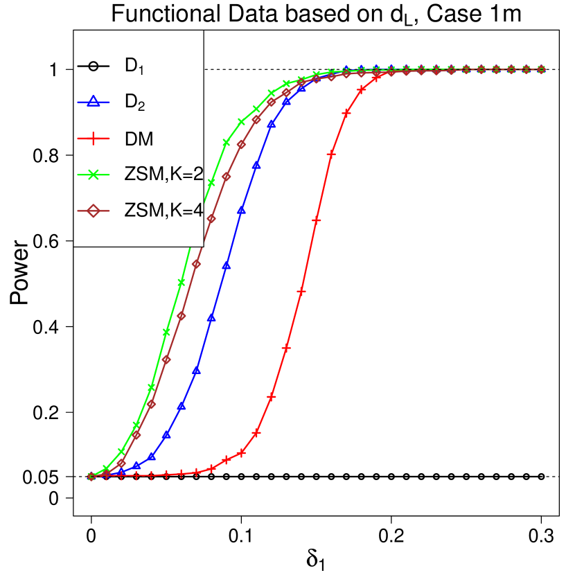
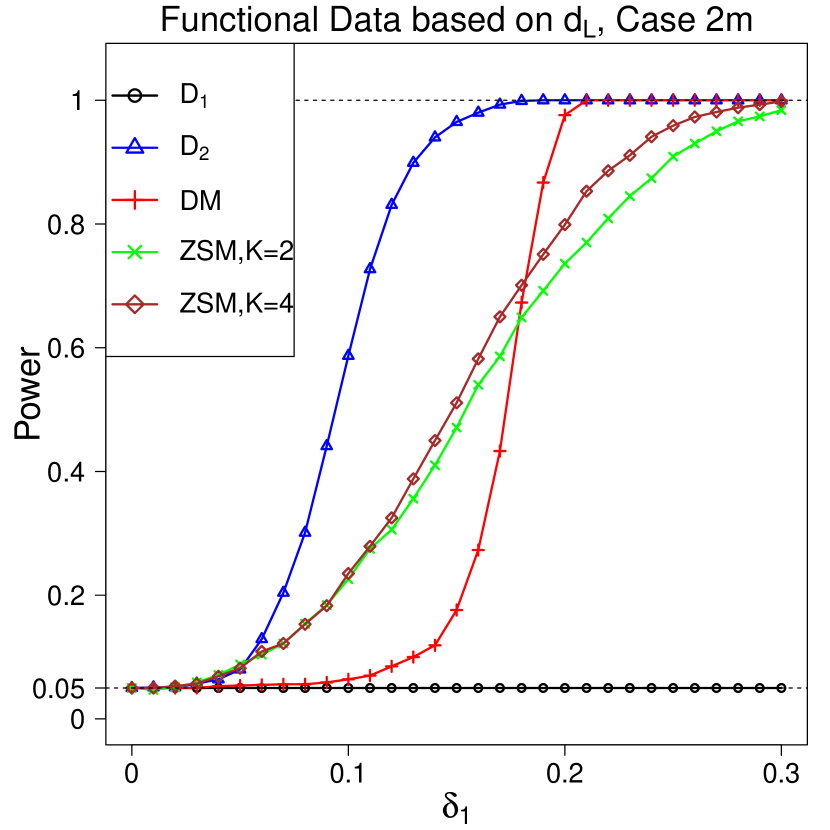
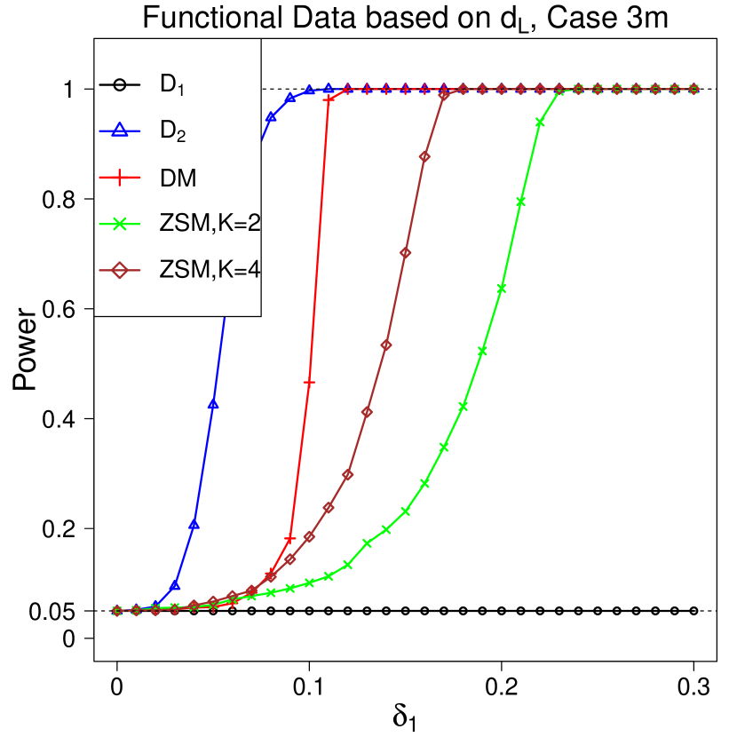
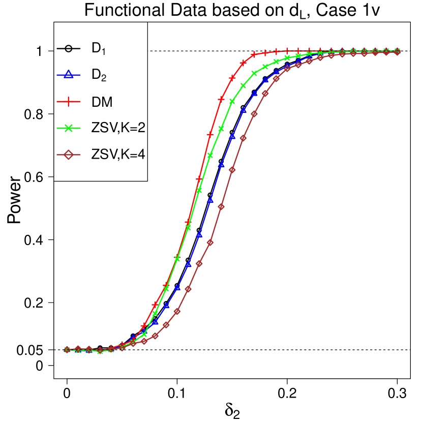
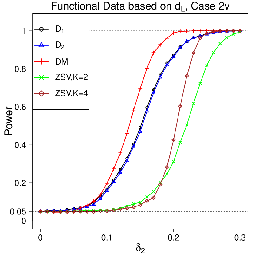
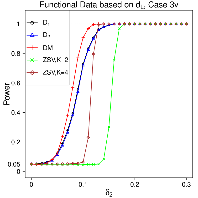
Figure 6: Size-Adjusted Power $(\times 100\%)$ at $\alpha=5\%$, $n_{i}=400$ and $\rho=0.4$. Upper panel: mean difference; bottom panel: covariance operator difference.

References

- (1)
- Andrews (1991) Andrews, D. W. (1991), ‘Heteroskedasticity and autocorrelation consistent covariance matrix estimation’, Econometrica: Journal of the Econometric Society pp. 817–858.
- Aue et al. (2018) Aue, A., Rice, G. & Sönmez, O. (2018), ‘Detecting and dating structural breaks in functional data without dimension reduction’, Journal of the Royal Statistical Society: Series B (Statistical Methodology) 80(3), 509–529.
- Berkes et al. (2013) Berkes, I., Horváth, L. & Rice, G. (2013), ‘Weak invariance principles for sums of dependent random functions’, Stochastic Processes and their Applications 123(2), 385–403.
- Billingsley (1968) Billingsley, P. (1968), Convergence of Probability Measures, John Wiley & Sons.
- Domínguez & Lobato (2000) Domínguez, M. A. & Lobato, I. N. (2000), ‘Size corrected power for bootstrap tests’, Instituto Technologico Autonomo de Mexico, Technical Notes .
- Dryden et al. (2009) Dryden, I. L., Koloydenko, A. & Zhou, D. (2009), ‘Non-Euclidean statistics for covariance matrices, with applications to diffusion tensor imaging’, The Annals of Applied Statistics 3(3), 1102–1123.
- Dubey & Müller (2019) Dubey, P. & Müller, H.-G. (2019), ‘Fréchet analysis of variance for random objects’, Biometrika 106(4), 803–821.
- Dubey & Müller (2020a) Dubey, P. & Müller, H.-G. (2020a), ‘Fréchet change-point detection’, The Annals of Statistics 48(6), 3312–3335.
- Dubey & Müller (2020b) Dubey, P. & Müller, H.-G. (2020b), ‘Functional models for time-varying random objects’, Journal of the Royal Statistical Society: Series B (Statistical Methodology) 82(2), 275–327.
- Dubey & Müller (2021) Dubey, P. & Müller, H.-G. (2021), ‘Modeling time-varying random objects and dynamic networks’, Journal of the American Statistical Association, to appear .
- Fréchet (1948) Fréchet, M. (1948), ‘Les éléments aléatoires de nature quelconque dans un espace distancié’, Annales de l’institut Henri Poincaré 10(4), 215–310.
- Fryzlewicz (2014) Fryzlewicz, P. (2014), ‘Wild binary segmentation for multiple change-point detection’, The Annals of Statistics 42(6), 2243–2281.
- Ginestet et al. (2017) Ginestet, C. E., Jun, L., Prakash, B., Steven, R. & Kolaczyk, E. D. (2017), ‘Hypothesis testing for network data in functional neuroimaging’, The Annals of Applied Statistics 11(2), 725–750.
- Hjort & Pollard (2011) Hjort, N. L. & Pollard, D. (2011), ‘Asymptotics for minimisers of convex processes’, arXiv preprint arXiv:1107.3806 .
- Jiang et al. (2022) Jiang, F., Zhao, Z. & Shao, X. (2022), ‘Modelling the COVID-19 infection trajectory: A piecewise linear quantile trend model’, Journal of the Royal Statistical Society: Series B (Statistical Methodology), in press .
- Mazzuco & Scarpa (2015) Mazzuco, S. & Scarpa, B. (2015), ‘Fitting age-specific fertility rates by a flexible generalized skew normal probability density function’, Journal of the Royal Statistical Society: Series A (Statistics in Society) 178(1), 187–203.
- Newey & West (1987) Newey, W. K. & West, K. D. (1987), ‘A simple, positive semi-definite, heteroskedasticity and autocorrelation consistent covariance matrix’, Econometrica 55(3), 703–708.
- Panaretos et al. (2010) Panaretos, V. M., Kraus, D. & Maddocks, J. H. (2010), ‘Second-order comparison of Gaussian random functions and the geometry of DNA minicircles’, Journal of the American Statistical Association 105(490), 670–682.
- Petersen & Müller (2019) Petersen, A. & Müller, H.-G. (2019), ‘Fréchet regression for random objects with Euclidean predictors’, The Annals of Statistics 47(2), 691–719.
- Pollard (1985) Pollard, D. (1985), ‘New ways to prove central limit theorems’, Econometric Theory 1(3), 295–313.
- Shang & Hyndman (2017) Shang, H. L. & Hyndman, R. J. (2017), ‘Grouped functional time series forecasting: An application to age-specific mortality rates’, Journal of Computational and Graphical Statistics 26(2), 330–343.
- Shao (2010) Shao, X. (2010), ‘A self-normalized approach to confidence interval construction in time series’, Journal of the Royal Statistical Society: Series B (Statistical Methodology) 72(3), 343–366.
- Shao (2015) Shao, X. (2015), ‘Self-normalization for time series: A review of recent developments’, Journal of the American Statistical Association 110(512), 1797–1817.
- Shao & Zhang (2010) Shao, X. & Zhang, X. (2010), ‘Testing for change points in time series’, Journal of the American Statistical Association 105(491), 1228–1240.
- Tucker et al. (2022) Tucker, D. C., Wu, Y. & Müller, H.-G. (2022), ‘Variable selection for global Fréchet regression’, Journal of the American Statistical Association, to appear .
- van der Vaart & Wellner (1996) van der Vaart, A. W. & Wellner, J. A. (1996), Weak convergence, in ‘Weak convergence and empirical processes’, Springer, pp. 16–28.
- Wang & Shao (2020) Wang, R. & Shao, X. (2020), ‘Hypothesis testing for high-dimensional time series via self-normalization’, The Annals of Statistics 48(5), 2728–2758.
- Wang et al. (2022) Wang, R., Zhu, C., Vogulshev, S. & Shao, X. (2022), ‘Inference for change points in high dimensional data via self-normalization’, The Annals of Statistics 50(2), 781–806.
- Zhang et al. (2022) Zhang, C., Kokoszka, P., & Petersen, A. (2022), ‘Wasserstein autoregressive models for density time series’, Journal of Time Series Analysis 43, 30–52.
- Zhang et al. (2021) Zhang, Q., Xue, L. & Li, B. (2021), ‘Dimension reduction and data visualization for Fréchet regression’, arXiv preprint arXiv:2110.00467 .
- Zhang & Lavitas (2018) Zhang, T. & Lavitas, L. (2018), ‘Unsupervised self-normalized change-point testing for time series’, Journal of the American Statistical Association 113(522), 637–648.
- Zhang & Shao (2015) Zhang, X. & Shao, X. (2015), ‘Two sample inference for the second-order property of temporally dependent functional data’, Bernoulli 21(2), 909–929.
- Zhang et al. (2011) Zhang, X., Shao, X., Hayhoe, K. & Wuebbles, D. (2011), ‘Testing the structural stability of temporally dependent functional observations and application to climate projections’, Electronic Journal of Statistics 5, 1765–1796.
- Zhou & Shao (2013) Zhou, Z. & Shao, X. (2013), ‘Inference for linear models with dependent errors’, Journal of the Royal Statistical Society: Series B (Statistical Methodology) 75(2), 323–343.
- Zhu & Müller (2021) Zhu, C. & Müller, H.-G. (2021), ‘Autoregressive optimal transport models’, arXiv preprint arXiv:2105.05439 .
- Zhu & Müller (2022) Zhu, C. & Müller, H.-G. (2022), ‘Spherical autoregressive models, with application to distributional and compositional time series’, arXiv preprint arXiv:2203.12783 .