Schiff moments of deformed nuclei.

Abstract

Stimulated by recent suggestion of Cosmic Axion Spin Precession Experiment with Eu contained compound we develop a new method for accurate calculation of Schiff moments of even-odd deformed nuclei. The method is essentially based on experimental data on magnetic moments and E1,E3-amplitudes in the given even-odd nucleus and in adjacent even-even nuclei. Unfortunately such sets of data are not known yet for most of interesting nuclei. Fortunately the full set of data is available for ¹⁵³Eu. Hence, we perform the calculation for ¹⁵³Eu and find value of the Schiff moment. The value is about 30 times larger than a typical Schiff moment of a spherical heavy nucleus. The enhancement of the Schiff moment in ¹⁵³Eu is related to the low energy octupole mode. On the other hand the value of Schiff moment we find is 30 times smaller than that obtained in the assumption of static octupole deformation.

I Introduction

Electric dipole moment (EDM) of an isolated quantum object in a nondegenerate quantum state is a manifestation of violation of time reversal (T) and parity (P) fundamental symmetries. Searches of EDM of neutron is a long quest for fundamental P,T-violation [1, 2, 3]. EDM of a nucleus can be significantly larger than that of a neutron [4]. However a nucleus has nonzero electric charge and therefore in a charge neutral system (atom, molecule, solid) EDM of nucleus cannot be measured [5]. The quantity that can be measured is the so called Schiff Moment (SM) which is nonzero due to the finite nuclear size [4]. Like EDM the SM is a vector directed along the angular momentum.

Renewal of my interest to this problem is related to Cosmic Axion Spin Precession Experiment (CASPEr) on searches of the QCD axion dark matter. The current CASPEr experiment is based on Lead Titanate ferroelectric [6], see also Ref. [7]. The experiment is probing the Schiff moment of ${}^{207}Pb$ nucleus. There is a recent suggestion [8] to use for CASPEr experiment the crystal of EuCl${}_{3}\cdot$ 6H₂O instead of Lead Titanate. The major advantage is experimental: a possibility to polarise Eu nuclei via optical pumping in this crystal allows to improve sensitivity by orders of magnitude. Expected effect in EuCl${}_{3}\cdot$ 6H₂O has been calculated in Ref. [9]. The observable effect in a solid is built like a Russian doll Matreshka, it has four different spatial and energy scales inside each other. (i) Quark-gluon scale, $r<1$fm, (ii) Nuclear scale, $1fm\lesssim r\lesssim 10fm$, (iii) Atomic scale, $10fm<r\lesssim 1\AA$, (iv) Solid state scale, $r>1\AA$. The calculation [9] is pretty accurate at the scale (iii), it has an uncertainty at most by factor 2 at the scales (i) and (iv). However, the uncertainty at the scale (ii), the nuclear scale, is two orders of magnitude, this is the uncertainty in ¹⁵³Eu Schiff moment. Such an uncertainty is more or less typical for deformed even-odd nuclei. The aim of the present work is twofold (i) development of the accurate method for SM calculation, (ii) performamce of the calculation for ¹⁵³Eu. A reliable purely theoretical calculation is hardly possible. Therefore, our appoach is to use available experimental data as much as posible.

¹⁵³Eu is a deformed nucleus. A simplistic estimate of SM of a nucleus with quadrupolar deformation based on Nilsson model performed in Ref. [4] gave a result by an order of magnitude larger than SM of a spherical heavy nucleus, say SM of ${}^{207}Pb$. It has been found later in Ref. [10] that if the nucleus has a static octupolar deformation the SM is dramatically enhanced. Based on analysis of rotational spectra of ¹⁵³Eu authors of Ref. [11] argued that ¹⁵³Eu has a static octupolar deformation and hence, using the idea [10] arrived to the estimate of SM that is $10^{3}$ times larger than that of a heavy spherical nucleus.

To elucidate structure of wave functions of ¹⁵³Eu in the present work we analyse available experimental data on magnetic moments and amplitudes of E1,E3-transitions. In the result of this analysis we confidently claim that the model of static octupolar deformation is too simplistic. Nilsson wave functions of quadrupolar deformed nucleus are almost correct. However, this does not imply that the octupolar mode is irrelevant. There is an admixture of the octupole vibration to the Nilsson states and we determine the amplitude of the admixture. All in all this allows us to perform a pretty reliable and accurate calculation of SM.

To avoid misundertanding, our statement about the magnitude of the SM is based on analysis of a broad set of data, therefore, the statement is nuclear specific, it is valid for ¹⁵³Eu and it is valid for ²³⁷Np. Unfortunately such sets of data are not known yet for many interesting nuclei.

Structure of the paper is the following. In Section II we analyse lifetimes of relevant levels in ¹⁵²Sm and ${}^{153}Eu$ and hence find the relevant E1-amplitudes. The Section III is the central one, here we discuss the structure of wave functions of the parity doublet $|5/2^{\pm}\rangle$ in ¹⁵³Eu. Section IV determines the quadrupolar deformation of ¹⁵³Eu. In Section V we explain the parametrisation we use for the octupolar deformation. Section VI describes the structure of octupole excitations. Section VII extracts the value of octupole deformation from experimental data. In section VIII we calculate the T- and P-odd mixing of $5/2^{+}$ and $5/2^{-}$ states in ¹⁵³Eu. EDM of ${}^{153}Eu$ nucleus is calculated in Section IX and SM of ${}^{153}Eu$ nucleus is calculated in Section X. Section XI presents our conclusions.

II Experimental E1-amplitudes in ${}^{152}Sm$ and ${}^{153}Eu$

All data in this Section are taken from Ref. [12]. Even-even nuclei in vicinity of ¹⁵³Eu have low energy $\approx 1$MeV collective octupole excitation. There is the quadrupolar ground state rotational band and the octupolar rotational band starting at energy of the octupole excitation. As a reference even-even nucleus we take ¹⁵²Sm. In principle ¹⁵⁴Sm also would do the job, but the data for ¹⁵⁴Sm are much less detailed, especially on electron scattering that we discuss in Section VII. Energies of the relevant states of the octupolar band in ¹⁵²Sm are: $E(1^{-})=963$keV, $E(3^{-})=1041$keV. The halftime of the $1^{-}$ state is $t_{1/2}=28.2$fs, hence the lifetime is $\tau=28.2/\ln(2)=40.7$fs. The state decays via the E1-transition to the ground state, $0^{+}$, and to the $2^{+}$ state of the ground state rotational band. The decay branching ratio is $W(0^{+})/W(2^{+})=0.823$. Therefore, the partial lifetime for $1^{-}\to 0^{+}$ transition is $\tau_{partial}=90$fs. The $1^{-}\to 0^{+}$ E1-transition decay rate is [13]

$$\frac{1}{\tau_{partial}}=\frac{4\omega^{3}}{3(2j+1)}|\langle j^{\prime}||d||j\rangle|^{2}\ ,$$ (1)

For $1^{-}\to 0^{+}$ transition $j=1$ and $j^{\prime}=0$. The reduced matrix element of the dipole moment can be expressed in terms of $d_{z}$ in the proper reference frame of the deformed nucleus [14]

$$|\langle j^{\prime}||d||j\rangle|^{2} = \left|\sqrt{(2j+1)(2j^{\prime}+1)}\left(\begin{array}[]{ccc}j^{\prime}&1&j\\ -m&0&m\end{array}\right)\right|^{2}$$ (4)

$$\times |\langle 0|d_{z}|1\rangle|^{2}$$ (5)

For $1^{-}\to 0^{+}$ transition $j=1$, $j^{\prime}=0$, $m=0$. Hence

$$\langle 0|d_{z}|1\rangle=+e\times 0.31fm$$ (6)

Here $e=|e|$ is the elementary charge.

${}^{153}Eu$ is a deformed nucleus with the ground state $|5/2^{+}\rangle$. The nearest opposite parity state $|5/2^{-}\rangle$ has energy $E=97.4$keV. The halftime of the $|5/2^{-}\rangle$ state is $t_{1/2}=0.20$ns, hence the lifetime is $\tau=0.29$ns. The lifetime is due to the E1-decay $|5/2^{-}\rangle\to|5/2^{+}\rangle$. Using Eqs.(1),(4) with $j=j^{\prime}=m=5/2$ and comparing with experiments we find the corresponding $d_{z}$ in the proper reference frame.

$$\langle 5/2^{+}|d_{z}|5/2^{-}\rangle=-e\times 0.12fm$$ (7)

Of course lifetimes do not allow to determine signs in Eqs. (6) and (7). We explain in Section VI how the signs are determined.

III Wave functions of the ground state parity doublet $|\frac{5}{2}^{\pm})$ in ${}^{153}Eu$.

The standard theoretical description of low energy states in ${}^{153}Eu$ is based on the Nilsson model of a quadrupolar-deformed nucleus. In agreement with experimental data, the model predicts the spin and parity of the ground state, $5/2^{+}$. It also predicts the existence of the low-energy excited state with opposite parity, $5/2^{-}$. The wave functions of the odd proton in the Nilsson scheme are $|5/2^{+}\rangle=|413\frac{5}{2}\rangle$, $|5/2^{-}\rangle=|532\frac{5}{2}\rangle$. Explicit form of these wave functions is presented in Appendix. There are two rotational towers built on these states.

An alternative to Nilsson approach is the model of static collective octupolar deformation [11]. In this model the odd proton moves in the pear shape potential forming the $\Omega=5/2$ single particle state. A single rotational tower built on this odd proton state is consistent with observed spectra and this is why the paper [11] argues in favour of static octupole deformation. However, two different parity rotational towers in Nilsson scheme are equally consistent with observed spectra. Therefore, based on spectra one can conclude only that both the Nilsson model and the static octupolar deformation model are consistent with spectra. One needs additional data to distinguish these two models.

The Nilsson model explains the value $\Omega=5/2$ while in the “static octupole” model this value pops up from nowhere. However, in principle it is possible that accidentally the single particle state in the pear shape potential has $\Omega=5/2$.

To resolve the issue “Nilsson vs octupole” we look at magnetic moments. The magnetic moment of the ground state is $\mu_{5/2^{+}}=1.53\mu_{N}$, see Ref. [12]. This value is consistent with prediction on the Nilsson model [15]. The magnetic moment of the $5/2^{-}$ state has some ambiguity, the measurement led to two possible interpretations, “the recommended value” $\mu_{5/2^{-}}=3.22\mu_{N}$, and another value consistent with measurement $\mu_{5/2^{-}}=-0.52\mu_{N}$, see Ref. [12]. The recommended value is consistent with the prediction of the Nilsson model [16]. Thus the magnetic moments are consistent with the Nilsson model and inconsistent with the octupole model which implies $\mu_{5/2^{-}}\approx\mu_{5/2^{+}}$.

While the arguments presented above rule out the static octupole model, they do not imply that the octupole is irrelevant, actually it is relevant. We will show now that while the Nilsson model explains magnetic moments it cannot explain E1-amplitudes.

Within the Nilsson model one can calculate the E1 matrix element $\langle 5/2^{+}|d_{z}|5/2^{-}\rangle$. A straightforward calculation with wave functions (51) gives the dipole matrix element

$$d_{z} = e(1-Z/A)\langle 532\frac{5}{2}|z|413\frac{5}{2}\rangle$$ (8)

$$= e(1-Z/A)\frac{z_{0}}{\sqrt{2}}(0.527-0.510+0.017)$$

$$= e\times 0.036fm\ .$$

Here we account the effective proton charge $(1-Z/A)=0.59$. The calculated matrix element (8) is 3 times smaller than the experimental one (7). The first impression is that the disagreement is not bad having in mind the dramatic compensations in Eq.(8). However, there are two following observations.
(i) It has been pointed out in Ref.[4] that the compensation in (8) is not accidental: the compensation is due to the structure of Nilsson states, and the matrix element $\langle 532\frac{5}{2}|z|413\frac{5}{2}\rangle$ is proportional to the energy splitting $\Delta E=E_{5/2^{-}}-E_{5/2^{+}}$. The matrix element is small because $\Delta E$ is small compared to the shell model energy $\omega_{0}\approx 7.7$MeV. The value (8) is calculated with wave functions from Ref. [17] that correspond to $\Delta E\approx 450$keV. On the other hand in reality $\Delta E\approx 97$keV. Therefore, the true matrix element must be even smaller than the value (8).
(ii) The electric dipole operator is T-even. Therefore, there is a suppression of the matrix element due to pairing of protons, $d_{z}\to d_{z}(u_{1}u_{2}-v_{1}v_{2})$, where $u$ and $v$ are pairing BCS factors. This further reduces the matrix element, see Ref.[18].

The arguments in the previous paragraph lead to the conclusion that while the Nilsson model correctly predicts quantum numbers and explains magnetic moments, the model does not explain the electric dipole transition amplitude. The experimental amplitude is by an order of magnitude larger than the Nilsson one. This observation has been made already in Ref.[4].

Admixture of the collective octupole to Nilsson states resolves the dipole moment issue. So, we take the wave functions as

$$|+\rangle=|\frac{5}{2}^{+}\rangle = \sqrt{1-\alpha^{2}}|413\frac{5}{2}\rangle|0\rangle-\alpha|532\frac{5}{2}\rangle|1\rangle$$

$$|-\rangle=|\frac{5}{2}^{-}\rangle = \sqrt{1-\alpha^{2}}|532\frac{5}{2}\rangle|0\rangle-\alpha|413\frac{5}{2}\rangle|1\rangle$$ (9)

Here the states $|0\rangle$ and $|1\rangle$ describe collective octupole mode, $|0\rangle$ is the symmetric octupole vibration and $|1\rangle$ is antisymmetric octupole vibration. For intuition: $|0\rangle$ corresponds to the ground state of ¹⁵²Sm and $|1\rangle$ corresponds to the octupole excitation at energy $\approx 1$MeV. We will discuss in Section VI the specific structure of the states $|0\rangle$, $|1\rangle$, explain why the mixing coefficient in both states in (III) is the same, and explain why $\alpha>0$.

Using (III) and neglecting the small single particle contribution the transition electric dipole moment is

$$\langle\frac{5}{2}^{+}|d_{z}|\frac{5}{2}^{-}\rangle=-2\alpha\sqrt{1-\alpha^{2}}\langle 0|d_{z}|1\rangle$$ (10)

Hence, using the experimental values (6) and (7) we find

$$\alpha\approx\frac{0.12}{2\times 0.31}=0.20$$ (11)

Thus, the weight of the admixture of the collective vibration to the simple Nilsson state is just $\alpha^{2}=4\%$. This weight is sufficiently small to make the Nilsson scheme calculation of magnetic moments correct. On the other hand the weight is sufficiently large to influence electric properties.

Note that the octupole vibration itself does not have an electric dipole transition matrix element. The E1 matrix element is zero due to elimination of zero mode, $\langle 1|d_{z}|0\rangle=0$. The nonzero value of the dipole matrix element, $\langle 1|d_{z}|0\rangle\neq 0$, arises due to a small shift of the neutron distribution with respect to the proton distribution in combination with the octupole deformation, see e.g. Refs. [19, 20, 21]. While this issue is important theoretically, pragmatically it is not important to us since we take both values of matrix elements (6) and (7) from experiment.

It is worth noting also that in the static octupole model one expects $\langle 5/2^{+}|d_{z}|5/2^{-}\rangle=\langle 0|d_{z}|1\rangle=+e\times 0.31fm$ that is like magnetic moments inconsistent with data.

IV Quadrupolar deformation of ${}^{153}Eu$.

The standard way to describe nuclear deformation is to use parameters $\beta_{l}$. In the co-rotating reference frame for the quadrupolar deformation the surface of the nucleus is given by equation (we neglect $\beta_{2}^{2}$ compared to 1)

$$R(\theta)=R_{0}(1+\beta_{2}Y_{2,0})$$

$$R_{0}=r_{0}A^{1/3}$$

$$r_{0}\approx 1.2fm$$ (12)

Here A is the number of nucleons.

Let us determine $\beta_{2}$ using the known electric quadrupole moment Q in the ground state of ¹⁵³Eu. There are two contributions in Q, (i) collective contribution due to the collective deformation, (ii) single particle contribution of the odd proton. Using Nilsson wave functions it is easy to check that the single particle contribution is about 3-4% of the experimental one, so it can be neglected. Collective electric quadrupole moment is given by density of protons $\rho_{p}$,

$$Q_{0}=Q_{zz} = \int\rho_{p}(3z^{2}-r^{2})dV=4\sqrt{\frac{\pi}{5}}\int\rho_{p}r^{2}Y_{20}dV$$ (13)

$$= \frac{3ZR_{0}^{2}}{\sqrt{5\pi}}\beta_{2}\left[1+\frac{2\sqrt{5}}{7\sqrt{\pi}}\beta_{2}+\frac{12}{7\sqrt{\pi}}\beta_{4}\right]$$

Here we also account $\beta_{4}$. Z is the nuclear charge. Eq.(13) gives the quadrupole moment in the proper reference frame. In the laboratory frame for the ground state, $J=\Omega=5/2$, the quadrupole moment is $Q=\frac{5}{14}Q_{0}$, see problem to $\S 119$ in Ref.[14]. The ground state quadrupole moment of ¹⁵³Eu is $Q=2.412$ barn [12]. From here, assuming $\beta_{4}=0.07$, we find the quadrupole deformation of ¹⁵³Eu nucleus in the ground state,

$$\beta_{2}\approx 0.29\ .$$ (14)

The values $\beta_{2}\approx 0.29$, $\beta_{4}=0.07$ perfectly agree with that in ¹⁵²Sm determined from electron scattering [22].

The electric quadrupole moment of ¹⁵¹Eu nucleus in the ground state is $Q=0.903$barn [12]. Therefore, in ¹⁵¹Eu the quadrupolar deformation, $\beta_{2}\approx 0.12$, is significantly smaller than that in ¹⁵³Eu.

V Nuclear density variation due to the octupole deformation

The standard way to describe the static octupole deformation $\beta_{3}$ is to use parametrisation (IV)

$$R(\theta)=R_{0}(1+\beta_{1}Y_{10}+\beta_{2}Y_{2,0}+\beta_{3}Y_{3,0}+...)$$ (15)

This Eq. describes the surface of nucleus in the proper reference frame. The dipole harmonic $Y_{10}$ is necessary to eliminate the zero mode, i.e. to satisfy the condition

$$\langle z\rangle=\int\rho(r)rY_{10}dV=0$$ (16)

where $\rho(r)$ is the number density of nucleons. From (16) we find

$$\beta_{1}=-x\beta_{2}\beta_{3}\ ,\ \ \ x=\sqrt{\frac{243}{140\pi}}\approx 0.743\ .$$ (17)

For our purposes it is more convenient to use parametrisation different from (15), the parametrisation we use is

$$\delta\rho=\beta_{3}\frac{3A}{4\pi R_{0}^{2}}\delta[r-R_{0}(1+\beta_{2}Y_{20})](Y_{30}-x\beta_{2}Y_{10})\ .$$ (18)

Here $\delta\rho$ is the octupolar component of the nuclear density. Due to the $\delta$-function, $\delta[...]$, the component is nonzero only at the surface of the nucleus. Parametrisations (15) and (18) are equivalent, both satisfy the constraint (16) and both give the same octupole moment

$$Q_{30}=\sqrt{\frac{4\pi}{7}}\int\rho r^{3}Y_{30}dV=\beta_{3}\frac{3A}{\sqrt{28\pi}}R_{0}^{3}\ .$$ (19)

VI Structure of the vibrational states $|0\rangle$, $|1\rangle$

The deformation picture described in the previous section is purely classical. Quantum mechanics makes some difference. We work in the proper reference frame where the nuclear axis direction, the z-axis, is fixed.

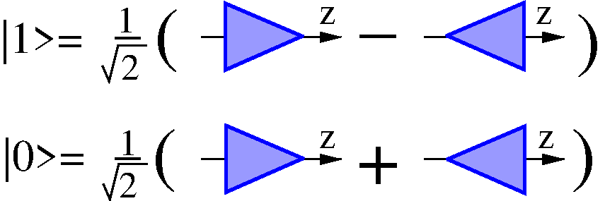
Figure 1: The states $|0\rangle$ and $|1\rangle$.

Hence, there are two possible orientations of the pear, as it is shown in Fig.1. There is tunnelling between these two orientations, the tunnelling leads to the energy splitting and to formations of symmetric and antisymmetric states $|0\rangle$, $|1\rangle$. This picture is valid when the tunnelling energy splitting, $\Delta E_{tun}$, is larger than the rotational energy splitting, $\Delta E_{rot}$. Experimentally $\Delta E_{tun}\sim 1$MeV, $\Delta E_{rot}\approx 20$keV, so the description is well justified. The description of Fig. 1 implies that the octupole deformation is quasistatic. The quasistatic description is justified by the existence of well defined rotational towers in ¹⁵²Sm built on $|0\rangle$ and $|1\rangle$ states, see Ref. [12]. Note that even if the pear tunneling amplitude is comparable with the rotatinal energy, $\Delta E_{tun}\sim\Delta E_{rot}$, the octupole deformation is not static. To have a trully static octupole one needs $\Delta E_{tun}\ll\Delta E_{rot}$.

The Hamiltonian for the odd proton reads

$$H=\frac{p^{2}}{2m}+U(r)\ .$$ (20)

Here $U(r)$ is the selfconsistent potential of the even-even core. It is well known that the nuclear density $\rho(r)$ has approximately the same shape as the potential

$$U(r)\approx\frac{U_{0}}{\rho(0)}\rho(r)\ ,$$ (21)

where $U_{0}\approx-50$MeV and $\rho(0)=3/(4\pi r_{0}^{3})$. Hence the variation of the potential related to the octupole deformation is

$$\delta U = \frac{U_{0}}{\rho(0)}\delta\rho$$

$$= \beta_{3}U_{0}R_{0}\delta[r-R_{0}(1+\beta_{2}Y_{20})](Y_{30}-x\beta_{2}Y_{10})\ .$$

This is the perturbation that mixes single particle Nilssen states with simultaneous mixing of $|0\rangle$ and $|1\rangle$. The mixing matrix element is

$$M=\langle 1|\langle 532\frac{5}{2}|\delta U|413\frac{5}{2}\rangle|0\rangle=\int\rho_{sp}(r)\delta U(r)dV$$

$$\rho_{sp}(r)=\langle\psi^{*}_{532}(r)\psi_{413}(r)\rangle\ .$$ (23)

Here $\rho_{sp}$ is offdiagonal single particle density of Nilsson wave functions (51), the density depends on $r$, the brackets $\langle..\rangle$ in $\rho_{sp}$ denote averaging over spin only. Numerical evaluation of the mixing matrix element is straightforward, the answer at $\beta_{2}=0.29$ is $M\approx 5\beta_{3}$MeV. The value slightly depends on $\beta_{2}$, at $\beta_{2}=0$ the value of M is 10% smaller. The coefficient $\alpha$ in Eqs.(III) is

$$\alpha=\frac{M}{\Delta E_{tun}}\ ,$$ (24)

where $\Delta E_{tun}\approx 1$MeV. Eqs.(24),(VI) together with positive value of M explain why the coefficient $\alpha$ is the same in both Eqs.(III) and why $\alpha>0$.

Moreover, comparing (24) with value of $\alpha$ extracted from experimental data, Eq.(11), we determine the octupole deformation, $\beta_{3}=0.04$. While the value is reasonable, unfortunately one cannot say that this is the accurate value. The shape approximation (21) is not very accurate. Even more important, it is not clear how the BCS factor influences $\rho_{sp}$. The BCS factor can easily reduce $\rho_{sp}$ by factor $\sim 2-3$, hence increasing $\beta_{3}$ by the same factor. Theoretical calculations of $\beta_{3}$ give values from 0.05 [21], to 0.075 [24], and even 0.15 [25].

VII The value of the octupole deformation parameter $\beta_{3}$

With wave functions shown in Fig.1 one immediately finds the electric octupole matrix element between states $|0\rangle$ and $|1\rangle$

$$\langle 1|Q_{30}^{(e)}|0\rangle=e\frac{Z}{A}Q_{30}\ ,$$ (25)

where $Q_{30}$ is given by Eq.(19). We are not aware of direct measurements of $Q_{30}^{(e)}$ in ${}^{152}Sm$. The book [17] presents the “oscillator strengths” for corresponding E3 transitions in ¹⁵²Sm and ²³⁸U, ${}^{152}Sm:\ B_{3}=1.2\times 10^{5}e^{2}fm^{6}$, ${}^{238}U:\ B_{3}=5\times 10^{5}e^{2}fm^{6}$ (table 6.14 in the book). However, these values have been determined not from direct electromagnetic measurements, the “oscillator strengths” have been indirectly extracted from deuteron scattering from the nuclei. Fortunately for ²³⁸U there is a more recent value determined from the electron scattering [23]: $B_{3}=(6.4\pm 0.6)\times 10^{5}e^{2}fm^{6}$. All in all this data give $\beta_{3}\approx 0.08$ for both ¹⁵²Sm and ²³⁸U.

Fortunately, the electron scattering data [22] allow to determine $\beta_{3}$ in ¹⁵²Sm pretty accurately. The Ref. [22] was aimed to determine $\beta_{2}$ and $\beta_{4}$, their results, $\beta_{2}=0.287\pm 0.003$, $\beta_{4}=0.070\pm 0.003$ are remarkably close to that we get for ¹⁵³Eu in Section IV. The inelastic scattering spectrum copied from Ref. [22] is shown in Fig.2.

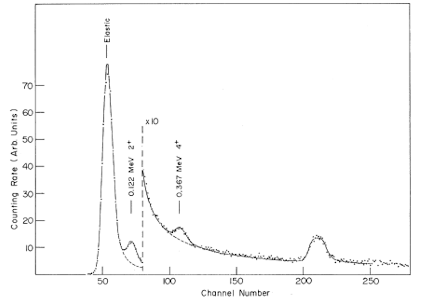
Figure 2: Spectrum of scattered electrons from ¹⁵²Sm at $93.5^{o}$. Incident electron energy, 76 MeV. Besides the ground-state rotational band, the $3^{-}$ level at 1. 041 MeV and the $2^{+}$ level at 1.086 MeV are seen (channel 210). The plot is taken from Ref. [22]

Here we reanalyse the spectrum. The first inelastic peak at E=122keV ($\approx$ channel 73) corresponds to the $2^{+}$ excitation of the rotational ground state band. The peak after subtraction of the background is shown in panel a of Fig.3.

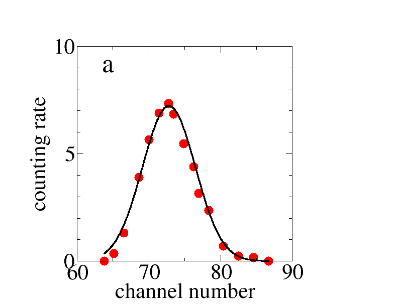
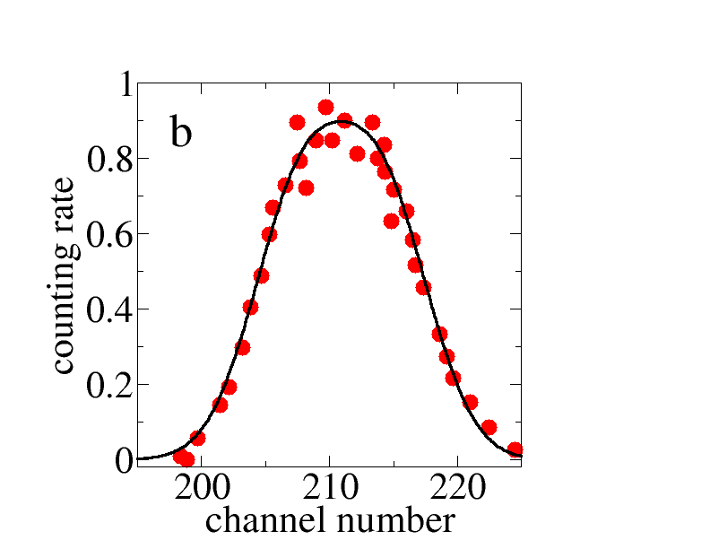
Figure 3: Excitation peaks with subtracted background. Red dots are experimental data and black curves are Gaussian (double Gaussian) fits. Panel a: The $2^{+}$ excitation of the ground state rotational band. Panel b: The combined peak of the $3^{-}$ octupole and the $\gamma 2^{+}$ state of the rotational $\gamma$-band.

Red dots are experimental points and the solid curve is the Gaussian fit

$$I=Ae^{-(x-x_{0})^{2}/\sigma^{2}}$$

$$A=7.23,\ x_{0}=72.9,\ \sigma=5.21\ .$$ (26)

Hence, the halfwidth is $\Gamma=2\ln(2)\sigma=49.3$keV. Here we account that one channel step is 6.82keV. This energy resolution is 0.065% of electron energy 76MeV. This is slightly smaller than the “typical value” 0.08% mentioned in Ref. [22]. The peak at Fig.2 near the channel 210 is a combination of the $3^{-}$ octupole (E=1041keV) and of the $\gamma 2^{+}$ state of the $\gamma$-band (E=1086keV). The peak after subtraction of the background is shown in panel b of Fig.3. We fit the double peak by the double Gaussian

$$I=B\left[e^{-(x-x_{1})^{2}/\sigma^{2}}+e^{-(x-x_{2})^{2}/\sigma^{2}}\right]$$

$$B=0.670,\ x_{1}=207.6,\ x_{2}=214.2,\ \sigma=5.21.$$ (27)

The value of $x_{1}$ corresponds to E=1041keV, the value of $x_{2}$ corresponds to E=1086keV, $\sigma$ is known from (VII). The fitting shows that intensities of $3^{-}$ and $\gamma 2^{+}$ lines cannot differ by more than 5%, so we take them equal. Therefore in the end there is only one fitting parameter B.

Based on Eqs.(VII) and (VII) we find the ratio of spectral weights

$$\frac{S(3^{-})}{S(2^{+})}=\frac{B}{A}=0.093$$ (28)

Here $2^{+}$ is the ground state rotational state. Interestingly, the analysis gives also the spectral weight of the $\gamma 2^{+}$ state. This allows to determine the magnituide of the $\gamma$-deformation. However, this issue is irrelevant to the Schiff moment and therefore we do not analyse it further.

Coulomb potential or Eu nucleus at $r\approx R_{0}$ is 15MeV. This is significantly smaller than the electron energy 76MeV. Therefore, the electron wavefunction can be considered as a plane wave. The momentum transfer is

$$q=2p\sin(93.5^{o}/2)\approx 111MeV\approx 0.562fm^{-1}\ .$$ (29)

Using expansion of the plane wave in spherical harmonics together with Wigner-Eckart theorem the spectral weights can be expressed as integrals in the co-rotating reference frame

$$S(2^{+}) \propto \left|\int Y_{20}j_{2}(qr)\rho(r)dV\right|^{2}$$

$$S(3^{-}) \propto \left|\int Y_{30}j_{3}(qr)\delta\rho(r)dV\right|^{2}$$ (30)

Here $j_{l}(qr)$ is the spherical Bessel function [14], $\rho(r)$ is the density with quadrupolar deformation, and $\delta\rho$ is given by Eq.(18). The coefficient of proportionality in both equations (VII) is the same and therefore we skip it. Evaluation of integrals in (VII) is straightforward, it gives

$$\int Y_{20}j_{2}(qr)\rho(r)dV\propto\beta_{2}j_{2}(qR_{0})=0.302\beta_{2}$$

$$\int Y_{30}j_{3}(qr)\delta\rho(r)dV\propto\beta_{3}j_{3}(qR_{0})=0.205\beta_{3}$$ (31)

Comparing the theoretical ratio with it’s experimental value (28) and using the known quadrupolar deformation we find the octupolar deformation $\beta_{3}=0.45\beta_{2}=0.130$.

In the previous paragraph we used the plane wave approximation for the electron wave function neglecting the Coulomb potential $\approx 15$MeV compared to the electron energy 76MeV. A simple way to estimate the Coulomb correction is to change $q\to q^{\prime}\approx q(1+15/76)=0.673fm^{-1}$. This results in $\beta_{3}=0.090$. Probably this simplistic way overestimates the effect of the Coulomb potential. An accurate calculation of distorted electron wave functions would allow to determine $\beta_{3}$ very accurately. For now we take

$$\beta_{3}=0.10$$ (32)

VIII T- and P-odd mixing of $5/2^{+}$ and $5/2^{-}$ states in ${}^{153}Eu$

The operator of the T, P-odd interaction reads [4]

$$H_{TP}=\eta\frac{G}{2\sqrt{2}m}{\vec{\sigma}}\cdot{\vec{\nabla}}\rho$$ (33)

Here $G\approx 1.03/m^{2}$ is the Fermi constant, $\eta$ is a dimensionless constant characterising the interaction, ${\vec{\sigma}}$ is the Pauli matrix corresponding to the spin of unpaired nucleon, and $\rho$ is the nuclear number density. The single particle matrix element of $H_{TP}$ between the Nilsson states can be estimated as, see Ref. [4],

$$\langle 532|H_{TP}|413\rangle\propto\langle 532|\nabla\rho|413\rangle\propto\langle 532|\nabla U|413\rangle$$

$$\propto\langle 532|[p,H]|413\rangle\propto(E_{532}-E_{413})\langle 532|p|413\rangle$$

$$\propto(E_{532}-E_{413})\langle 532|[r,H]|413\rangle$$

$$\propto(E_{532}-E_{412})^{2}\langle 532|r|413\rangle$$

Thus, the matrix element is suppressed by the small parameter $(\Delta E/\omega_{0})^{2}$, with $\Delta E\approx 100$keV and $\omega_{0}\approx 8$MeV. Hence, the single particle matrix element can be neglected.

The matrix element between the physical states (III) contains also the collective octupole contribution

$$\langle-|H_{TP}|+\rangle= -\alpha\langle 532\frac{5}{2}|\langle 1|H_{TP}|0\rangle|532\frac{5}{2}\rangle$$ (34)

$$-\alpha\langle 413\frac{5}{2}|\langle 0|H_{TP}|1\rangle|413\frac{5}{2}\rangle$$

Integrating by parts we transform this to

$$\langle-|H_{TP}|+\rangle = \frac{\alpha\eta G}{2\sqrt{2}m}\int\left[\rho_{532}(r)+\rho_{413}\right]\delta\rho(r)dV$$

$$\rho_{532}(r) = \partial_{z}\langle 532|\sigma_{z}|532\rangle$$

$$\rho_{413}(r) = \partial_{z}\langle 413|\sigma_{z}|413\rangle$$ (35)

Here $\delta\rho$ is the octupole density (18). Note that the “spin densities” $\rho_{532}$ and $\rho_{413}$ depend on $r$, the brackets $\langle..\rangle$ in definition of the densities in (VIII) denote averaging over spin only. Note also that the “spin densities” are T-odd. Therefore, the BCS factor practically does not influence them. Numerical evaluation of integrals in (VIII) with Nilsson wave functions (51) is straightforward, the result is

$$\langle-|H_{TP}|+\rangle = \alpha\eta\beta_{3}\frac{G}{2\sqrt{2}m}\frac{3A}{4\pi R_{0}^{4}}[I_{413}+I_{532}]$$ (36)

Dimensionless $I_{413}$ and $I_{532}$ are plotted in Fig.4 versus $\beta_{2}$.

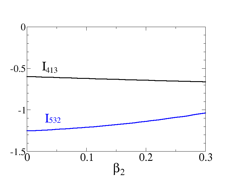
Figure 4: Dimensionless matrix elements $I_{413}$ and $I_{532}$ vs quadrupolar deformation.

At the physical deformation, $\beta_{2}=0.29$, Eq.(14), the values are $I_{413}=-0.66$ and $I_{532}=-1.05$. Hence we arrive to the following mixing matrix element

$$\langle-|H_{TP}|+\rangle=-0.24\alpha\eta\beta_{3}\ eV\ .$$ (37)

IX Electric dipole moment of ${}^{153}Eu$ nucleus

We need to determine signs in Eq.(6) and Eq.(7). In our notations $\beta_{3}>0$ corresponds to the pear orientation with respect to the z-axis shown in Fig.5.

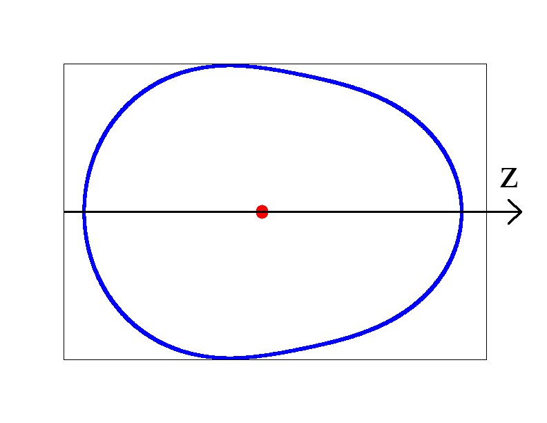
Figure 5: Pear shape with $\beta_{2}=0.29$, $\beta_{3}=0.10$

According to Refs. [19, 20, 21] protons are shifted in the positive z-direction. Hence, $d_{z}$ in Eq.(6) is positive. Hence, using Eqs.(III), we conclude that the sign in Eq.(7) is negative.

With Eqs.(37) and (7) we find the T,P-odd electric dipole moment in the ground state.

$$d^{TP}_{z} = 2\frac{\langle+|d_{z}|-\rangle\langle-|H_{TP}|+\rangle}{E_{+}-E_{-}}$$ (38)

$$= -0.59\times 10^{-6}\alpha\beta_{3}\eta[e\cdot fm]$$

$$= -1.18\times 10^{-8}\eta[e\cdot fm]\ .$$

For the numerical value we take $\alpha=0.20$, see Eq.(11), and $\beta_{3}=0.10$, see Eq.(32). Eq. (38) gives the EDM in the co-rotating reference frame. The EDM in the laboratory reference frame is

$$d^{TP}=\frac{5}{7}d^{TP}_{z}=-0.84\times 10^{-8}\eta[e\cdot fm]$$ (39)

This EDM is comparable with that of a heavy spherical nucleus, see Ref. [4]

X Schiff moment of ${}^{153}Eu$ nucleus

The operator of the Schiff moment (SM) reads [4]

$${\hat{S}}_{z}=\frac{1}{10}\left[\int\rho_{q}r^{2}zdV-\frac{5}{3}r_{q}^{2}d_{z}\right]$$ (40)

It is a vector. Here $\rho_{q}$ is the charge density and

$$r_{q}^{2}\approx\frac{3}{5}R_{0}^{2}$$ (41)

is the rms electric charge radius squared. With the static octupole deformation (18) the 1st term in (40) is

$$S_{intr}=\frac{1}{10}\int\rho_{q}r^{2}zdV=\frac{9}{20\sqrt{35}\pi}eZR_{0}^{3}\beta_{2}\beta_{3}$$ (42)

Here we use the same notation $S_{intr}$ as that in Refs.[26, 11]. The matrix element of the first term in (40) between the states (III) is

$$\langle+|{\hat{S}}_{1z}|-\rangle = -2\alpha S_{intr}$$ (43)

$$= -\alpha\frac{9}{10\pi\sqrt{35}}eZR_{0}^{3}\beta_{2}\beta_{3}$$

Combining this with Eq.(37) we find the expectation value over the ground state

$$\langle+|{\hat{S}}_{1z}|+\rangle = 2\frac{\langle+|{\hat{S}}_{1z}|-\rangle\langle-|H_{TP}|+\rangle}{E_{+}-E_{-}}$$ (44)

$$= -0.24\times 10^{-6}eZR_{0}^{3}\alpha^{2}\beta_{2}\beta_{3}^{2}\eta$$

Hence, the Schiff moment is

$$S_{z} = \langle+|{\hat{S}}_{z}|+\rangle=\langle+|{\hat{S}}_{1z}|+\rangle-\frac{1}{10}R_{0}^{2}d_{z}^{TP}$$ (45)

$$= \left[-4.0\times 10^{-3}\alpha^{2}\beta_{2}\beta_{3}^{2}+2.4\times 10^{-6}\alpha\beta_{3}\right]\eta[e\cdot fm^{3}]$$

$$= -4.16\times 10^{-7}\eta[e\cdot fm^{3}]$$

For the final numerical value we take $\alpha=0.20$, see Eq.(11), $\beta_{2}=0.29$, see Eq.(14) and $\beta_{3}=0.10$, see Eq.(32). Note that the first term in the middle line of Eq.(45) is proportional to $\alpha^{2}\beta_{3}^{2}$ and at the same time the second term is proportional to $\alpha\beta_{3}$. This is because one power of $\alpha\beta_{3}$ is “hidden” in the experimental dipole matrix element (7). The second term is just about 10% of the first one. Eq. (45) gives the Schiff moment in the co-rotating reference frame. The Schiff moment in the laboratory reference frame is

$$S=\frac{5}{7}S_{z}=-2.97\times 10^{-7}\eta[e\cdot fm^{3}]$$ (46)

This result is pretty reliable, the major uncertainty about factor 2 is due to uncertainty in the value of $\beta_{3}$. A more accurate analysis of inelastic electron scattering data [22], see Section V, can reduce the uncertainty.

In ¹⁵¹Eu the energy splitting $E_{-}-E_{+}$ is 3.5 times larger than that in ¹⁵³Eu, and the quadrupolar deformation is 2.5 times smaller. Therefore, the Schiff moment is at least an order of magnitude smaller than that of ¹⁵³Eu. Unfortunately, there is no enough data for an accurate calculation for ¹⁵¹Eu.

Another interesting deformed nucleus is ²³⁷Np. Performing a simple rescaling from our result for ¹⁵³Eu we get the following estimate of ²³⁷Np Schiff Moment, $S\sim-1.5\times 10^{-6}\eta[e\cdot fm^{3}]$. This is 40 times larger than the single particle estimate [4]. Of course following our method and using ²³⁸U as a reference nucleus (like the pair ¹⁵³Eu, ¹⁵²Sm in the present work) one can perform an accurate calculations of ²³⁷Np Schiff moment. Data for ²³⁸U are available in Ref. [23].

XI Conclusions

The Hamiltonian of nuclear time and parity violating interaction is defined by Eq.(33). For connection of the dimensionless interaction constant $\eta$ with the QCD axion $\theta$-parameter see Ref. [9]. The Hamiltonian (33) leads to the Schiff moment of a nucleus. In the present work we have dveloped a new method to calculate Schiff moment of an even-odd deformed nucleus. The method is essentially based on experimental data on magnetic moments and E1,E3-amplitudes in the given even-odd nucleus and in adjacent even-even nuclei. Unfortunately such sets of data are not known yet for most of interesting nuclei. Fortunately the full set of necessary data exists for ¹⁵³Eu. Hence, using the new method, we perform the calculation for ¹⁵³Eu. The result is given by Eq.(46). The theoretical uncertainty of this result, about factor 2, is mainly due to the uncertainty in the value of the octupole deformation. A more sophisticated analysis of available electron scattering data can further reduce the uncertainty.

The Schiff Moment (46) is about 20-50 times larger than that in heavy spherical nuclei [4] and it is 3 times larger than what paper [9] calls “conservative estimate”. On the other hand it is by factor 30 smaller than the result of Ref. [11] based on the model of static octupole deformation.

Using the calculated value of the Schiff Moment we rescale results of Ref. [9] for the energy shift of ¹⁵³Eu nuclear spin and for the effective electric field in EuCl${}_{3}\cdot$ 6H₂O compound. The result of the rescaling is

$$\delta{\cal E}_{o}=0.9\times 10^{-9}\theta[eV]$$

$$E_{o}^{*}=0.3MV/cm$$ (47)

These are figures of merit for the proposed [8] Cosmic Axion Spin Precession Experiment with EuCl${}_{3}\cdot$ 6H₂O.

Appendix A Nilsson wave functions

Parameters of the deformed oscillator potential used in Nilsson model are

$$\omega_{z}=\omega_{0}\left(1-\frac{2}{3}\delta\right),\ \ \ \ z_{0}=\frac{1}{\sqrt{m\omega_{z}}}$$

$$\omega_{\rho}=\omega_{0}\left(1+\frac{1}{3}\delta\right),\ \ \ \ \rho_{0}=\frac{1}{\sqrt{m\omega_{\rho}}}$$

$$\omega_{0}=\frac{41MeV}{A^{1/3}}$$ (48)

where $m\approx 940$MeV is the nucleon mass. The parameter $\delta$ is related $\beta_{2}$ used in the main text as

$$\delta=\frac{3\sqrt{5}}{4\sqrt{\pi}}\beta_{2}\approx 0.946\beta_{2}\ .$$ (49)

The oscillator wave functions defined in Ref. [17] are

$${\overline{z}} = z/z_{0}$$

$$|0\rangle_{z} = \frac{1}{(\sqrt{\pi}z_{0})^{1/2}}e^{-{\overline{z}}^{2}/2}$$

$$|1\rangle_{z} = \frac{\sqrt{2}}{(\sqrt{\pi}z_{0})^{1/2}}{\overline{z}}e^{-{\overline{z}}^{2}/2}$$

$$|2\rangle_{z} = \frac{1}{(2\sqrt{\pi}z_{0})^{1/2}}[2{\overline{z}}^{2}-1]e^{-{\overline{z}}^{2}/2}$$

$$|3\rangle_{z} = \frac{1}{(3\sqrt{\pi}z_{0})^{1/2}}{\overline{z}}[2{\overline{z}}^{2}-3]e^{-{\overline{z}}^{2}/2}$$

$${\overline{\rho}} = \rho/\rho_{0}$$

$$|2,2\rangle_{\rho} = \frac{1}{\sqrt{2\pi}\rho_{0}}{\overline{\rho}}^{2}e^{-{\overline{\rho}}^{2}/2}e^{2i\varphi}$$

$$|3,3\rangle_{\rho} = \frac{1}{\sqrt{6\pi}\rho_{0}}{\overline{\rho}}^{3}e^{-{\overline{\rho}}^{2}/2}e^{3i\varphi}$$

$$|4,2\rangle_{\rho} = \frac{1}{\sqrt{6\pi}\rho_{0}}{\overline{\rho}}^{2}({\overline{\rho}}^{2}-3)e^{-{\overline{\rho}}^{2}/2}e^{2i\varphi}$$

$$|5,3\rangle_{\rho} = \frac{1}{\sqrt{24\pi}\rho_{0}}{\overline{\rho}}^{3}({\overline{\rho}}^{2}-4)e^{-{\overline{\rho}}^{2}/2}e^{3i\varphi}$$ (50)

The Nilsson wave functions for the quadrupolar deformation $\delta=0.3$ written the oscillator basis (A) are [17]

$$|413\frac{5}{2}\rangle = 0.938|1\rangle_{z}|3,3\rangle_{\rho}|\downarrow\rangle-0.342|2\rangle_{z}|2,2\rangle_{\rho}|\uparrow\rangle$$ (51)

$$+ 0.054|0\rangle_{z}|4,2\rangle_{\rho}|\uparrow\rangle$$

$$|532\frac{5}{2}\rangle = 0.861|3\rangle_{z}|2,2\rangle_{\rho}|\uparrow\rangle+0.397|2\rangle_{z}|3,3\rangle_{\rho}|\downarrow\rangle$$

$$+ 0.310|1\rangle_{z}|4,2\rangle_{\rho}|\uparrow\rangle+0.075|0\rangle_{z}|5,3\rangle_{\rho}|\downarrow\rangle$$

References

- [1] N. F. Ramsey, Ann. Rev. Nucl. Part. Sci. 32, 211 (1982).
- [2] A. P. Serebrov et al, Physics of Particles and Nuclei Letters 12, 286 (2015).
- [3] C. Abel et al., Physical Review Letters 124, 081803 (2020), arXiv:2001.11966.
- [4] O. P. Sushkov, V V Flambaum, and I B Khriplovich. Sov. Phys. JETP 60,873 (1984).
- [5] L. I. Schiff, Physical Review 132, 2194 (1963).
- [6] D. Budker, P. W. Graham, M. Ledbetter, S. Rajendran, and A. O. Sushkov, Phys. Rev. X 4, 21030 (2014).
- [7] T. N. Mukhamedjanov and O. P. Sushkov, Physical Review A 72, 34501 (2005).
- [8] A. O. Sushkov, arXiv:2304.12105.
- [9] A. O. Sushkov, O. P. Sushkov, A. Yaresko, Phys. Rev. A 107, 062823 (2023); arxiv 2304.08461.
- [10] N. Auerbach, V. V. Flambaum, and V. Spevak, Physical Review Letters, 76, 4316 (1996).
- [11] V. V. Flambaum and H. Feldmeier. Phys. Rev. C 101, 015502 (2020).
- [12] Richard B Firestone. Table of Isotopes. Ed. by S Y Frank Chu and Coral M Baglin. 1999.
- [13] Quantum Electrodynamics: Volume 4 (Course of Theoretical Physics) 2nd Edition by V B Berestetskii, E.M. Lifshitz, and L. P. Pitaevskii.
- [14] Quantum Mechanics: Non-Relativistic Theory 3rd Edition by L. D. Landau, E. M. Lifshitz.
- [15] I. L. Lamm, Nuclear Physics A 125, 504 (1969).
- [16] E. Kemah, E. Tabar, H. Yakut, G. Hosgor https://dergipark.org.tr/en/pub/saufenbilder/article/1123474
- [17] Aage Bohr and Ben R. Mottelson. Nuclear Structure. World Scientific, 1998
- [18] O. P. Sushkov and V. B. Telitsin, Phys. Rev. C 48, 1069 (1993).
- [19] G. A. Leander, W. Nazarewicz, G. F. Bertsch, and J. Dudek, Nucl. Phys. A 453, 58 (1986).
- [20] C. O. Dorso, W. D. Myers, and W. J. Swiatecki, Nucl. Phys. A 451, 189 (1986).
- [21] P. A. Butler and W. Nazarewicz, Nucl. Phys. A 533, 249 (1991).
- [22] W. Bertozzi, T. Cooper, N. Ensslin, J. Heisenberg, S. Kowalski, M. Mills, W. Turchinetz, C. Williamson, S. P. Fivozinsky, J. W. Lightbody, Jr., and S. Penner, Phys. Rev. Lett. 28, 1711 (1972).
- [23] A. Hirsch, C. Creswell, W. Bertozzi, J. Heisenberg, M. V. Hynes, S. Kowalski, H. Miska, B. Norum, F. N. Had, C. P. Sargent, T. Sasanuma, and W. Turchinetz, Rev. Lett. 40, 632 (1978).
- [24] S. Ebata and T. Nakatsukasa Physica Scripta 92, 064005 (2017).
- [25] W. Zhang, Z. P. Li, S. Q. Zhang, and J. Meng, Phys. Rev. C 81, 034302 (2010).
- [26] V. Spevak, N. Auerbach, and V. V. Flambaum. Phys. Rev. C 56, 1357 (1997).