Mx2M: Masked Cross-Modality Modeling in Domain Adaptation for 3D Semantic Segmentation

Abstract

Existing methods of cross-modal domain adaptation for 3D semantic segmentation predict results only via 2D-3D complementarity that is obtained by cross-modal feature matching. However, as lacking supervision in the target domain, the complementarity is not always reliable. The results are not ideal when the domain gap is large. To solve the problem of lacking supervision, we introduce masked modeling into this task and propose a method Mx2M, which utilizes masked cross-modality modeling to reduce the large domain gap. Our Mx2M contains two components. One is the core solution, cross-modal removal and prediction (xMRP), which makes the Mx2M adapt to various scenarios and provides cross-modal self-supervision. The other is a new way of cross-modal feature matching, the dynamic cross-modal filter (DxMF) that ensures the whole method dynamically uses more suitable 2D-3D complementarity. Evaluation of the Mx2M on three DA scenarios, including Day/Night, USA/Singapore, and A2D2/SemanticKITTI, brings large improvements over previous methods on many metrics.

1 Introduction

3D semantic segmentation methods (Graham, Engelcke, and Van Der Maaten 2018; Wang et al. 2019; Hu et al. 2021) often encounter the problem of shift or gap between different but related domains (e.g. day and night). The task of cross-modal domain adaptation (DA) for 3D segmentation (Jaritz et al. 2020) is designed to address the problem, which is inspired by 3D datasets usually containing 2D and 3D modalities. Like most DA tasks, labels here are only available in the source domain, whereas the target domain has no segmentation labels. Existing methods, i.e. xMUDA (Jaritz et al. 2020) and its heirs (Liu et al. 2021a; Peng et al. 2021), extract 2D and 3D features through two networks and exploit the cross-modal complementarity by feature matching to predict results. However, as lacking supervision in the target domain, the robustness of this complementarity is not good. As shown in the left part of Fig.1, if the domain gap is large and both networks underperform on the target domain, these methods appear weak.

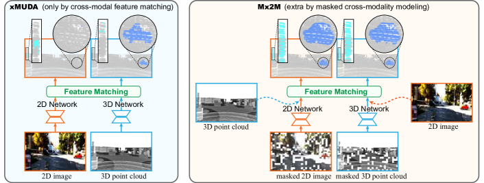
Figure 1: Left: the pipeline of xMUDA and its heirs (the segmentation results are from xMUDA). Right: the pipeline of our Mx2M. Thanks to masked cross-modality modeling, our method reduces the large domain gap and then achieves better segmentation results with the same backbone.

The problem of lacking supervision once constricted the visual pre-training task and has been solved by methods with masked modeling (He et al. 2022; Bao, Dong, and Wei 2022; Yu et al. 2022), which has been proved to belong to data augmentation (Xu et al. 2022). Its core solution is simple: removing a portion of inputs and learning to predict the removed contents. Models are fitted with sufficient data in this way, so that learn more inner semantic correspondences and realize self-supervision (He et al. 2022). For this DA task, this way of data augmentation and then the self-supervision can enrich the robustness and reduce the gap. Hence the idea is natural: if we introduce masked modeling into the task, the lacking supervision on the target domain and then the large gap are solved. Nevertheless, two problems are the key to introducing masked modeling. a) The core solution ought to be re-designed to fit for this task, where there are two modalities. b) For the cross-modal feature matching, we should explore a new way to suit the joining of masked modeling.

Given these observations, we propose a new method Mx2M utilizing masked cross-modality modeling to solve the problem of lacking supervision for the DA of 3D segmentation. Our Mx2M can reduce the large domain gap by adding two new components to the common backbone for this task, which correspond to the above two problems. For the first one, we design the core solution in the Mx2M, cross-modal removal and prediction (xMRP). As the name implies, we inherit the ’removal-and-prediction’ proceeding in the core solution of masked single-modality modeling and improve it with the cross-modal working manner for this task. During removal, the xMRP has two changes. i) Our CNN backbone cannot perform well with highly destroyed object shapes (Geirhos, Meding, and Wichmann 2020), so the masked portion is less. ii) To guarantee the existence of full semantics in this segmentation task, we do not mask all inputs and ensure at least one modality complete in each input. We can obtain the different xMRP by controlling the removal proceeding, which makes the Mx2M adapt to various DA scenarios. During prediction, to learn more 2D-3D correspondences beneficial to networks (Jaritz et al. 2020), we mask images/points and predict the full content in points/images by two new branches. In this way, cross-modal self-supervision can be provided for the whole method.

As for the second problem, we propose the dynamic cross-modal filter (DxMF) to dynamically construct the cross-modal feature matching by locations, which is inspired by impressive gains when dynamically establishing kernel-feature correspondences in SOLO V2 (Wang et al. 2020b). Similarly, in our DxMF, we structure the 2D-3D kernel-feature correspondences. Kernels for one modality are generated by features from the other, which then act on features for this modality and generate the segmentation results by locations. With the joining of the DxMF, the Mx2M can dynamically exploit the complementarity between modalities. As is shown in the right part of Fig.1, with these two components, our Mx2M gains good results even in the scenario with a large domain gap.

To verify the performance of the proposed Mx2M, we test it on three DA scenarios in (Jaritz et al. 2020), including USA/Singapore, Day/Night, and A2D2/SemanticKITTI. Our Mx2M attains better results compared with most state-of-the-art methods, which indicates its effectiveness. In summary, our main contributions are as follows:

• We innovatively propose a new method Mx2M, which utilizes masked cross-modality modeling to reduce the large domain gap for DA of 3D segmentation. To our knowledge, it is the first time that masked modeling is introduced into a cross-modal DA task.

• Two components are specially designed for this task, including xMRP and DxMF, which ensures the Mx2M effectively works and deals with various scenarios.

• We achieve high-quality results on three real-to-real DA scenarios, which makes the Mx2M the new state-of-the-art method. The good results demonstrate its practicality.

2 Related Work

Domain Adaptation for 3D Segmentation.

Most works pay attention to DA for 2D segmentation (Zhang et al. 2021, 2020; Li, Yuan, and Vasconcelos 2019), which are hard to be applied to unstructured and unordered 3D point clouds. The DA methods for 3D segmentation (Qin et al. 2019; Luo et al. 2020; Morerio, Cavazza, and Murino 2018) are relatively few, but they also do not fully use the datasets that often contain both images and points. Hence, xMUDA (Jaritz et al. 2020) and its heirs (Liu et al. 2021a; Peng et al. 2021) with cross-modal networks are proposed, which achieve better adaptation. Our Mx2M also adopts cross-modal networks, which has the same backbone as xMUDA.

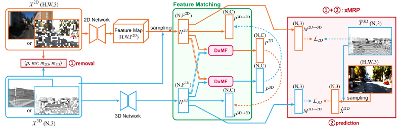
Figure 2: The architecture of the Mx2M. We introduce masked modeling into the task of DA in 3D segmentation mainly by xMRP and DxMF. The former is the core solution where we remove (mask) images/points and predict the full content in points/images. The latter is for 2D-3D feature matching.

Masked Modeling.

The masked modeling was first applied as masked language modeling (Kenton and Toutanova 2019), which essentially belongs to data augmentation (Xu et al. 2022). Nowadays, it has been the core operation in self-supervised learning for many modalities, such as masked image modeling (Bao, Dong, and Wei 2022; Xie et al. 2022), masked point modeling (Yu et al. 2022), and masked speech modeling (Baevski et al. 2020). Their solutions are the same: removing a portion of the data and learning to predict the removed content. The models are fitted with sufficient data in this way so that the lacking of supervision is satisfied. Our Mx2M designs the masked cross-modality modeling for DA in 3D segmentation that uses point and image.

Cross-modal Learning.

Cross-modal learning aims at taking advantage of data from multiple modalities. For visual tasks, the most common scene using it is learning the 3D task from images and point clouds (Jing, Zhang, and Tian 2021; Hu et al. 2021; Genova et al. 2021; Liu et al. 2021b; Xu et al. 2021; Dai and Nießner 2018; Liu, Qi, and Fu 2021). The detailed learning means are various, including 2D-3D feature matching (Jing, Zhang, and Tian 2021; Dai and Nießner 2018; Liu, Qi, and Fu 2021; Xu et al. 2021), 2D-3D feature fusion (Hu et al. 2021), 2D-3D cross-modal supervision (Genova et al. 2021; Liu et al. 2021b), etc. Besides, there are also some works conducting cross-modal learning on other modalities, such as video and medical image (Carreira and Zisserman 2017; Shan et al. 2018), image and language (Lu et al. 2021; Radford et al. 2021; Fu et al. 2021), as well as video and speech (Gao and Grauman 2021; Lee et al. 2021; Wu et al. 2022). Cross-modal learning is also exploited in our M2xM: the core procedure xMRP leverages the cross-modal supervision, while the DxMF works in the way of 2D-3D feature matching.

3 Method

Our Mx2M is designed for DA in 3D segmentation assuming the presence of 2D images and 3D point clouds, which is the same as xMUDA (Jaritz et al. 2020). For each DA scenario, we define a source dataset $\mathcal{S}$, each sample of which contains a 2D image $X^{\rm{2D,S}}$, a 3D point cloud $X^{\rm{3D,S}}$, and a corresponding 3D segmentation label $Y^{\rm{3D,S}}$. There also exists a target dataset $\mathcal{T}$ lacking annotations, where each sample only consists of image $X^{\rm{2D,T}}$ and point cloud $X^{\rm{3D,T}}$. The images and point clouds in $\mathcal{S}$ and $\mathcal{T}$ are in the same spatial sizes, i.e. $X^{\rm{2D}}\in\mathbb{R}^{\rm{H}\times\rm{W}\times 3}$ and $X^{\rm{3D}}\in\mathbb{R}^{\rm{N}\times 3}$. Based on these definitions, we will showcase our Mx2M.

3.1 Network Architecture

The architecture of the Mx2M is shown in Fig.2. For a fair comparison with previous methods (Jaritz et al. 2020; Liu et al. 2021a; Peng et al. 2021), we also use the same backbone to extract features: a SparseConvNet (Graham, Engelcke, and Van Der Maaten 2018) for the 3D network and a modified version of U-Net (Ronneberger, Fischer, and Brox 2015) with ResNet-34 (He et al. 2016) pre-trained on ImageNet (Deng et al. 2009) for the 2D one. Their output features, $H^{\rm{2D}}$ and $H^{\rm{3D}}$, have the same length N equaling the number of 3D points, where $H^{\rm{2D}}$ is gained by projecting the points into the image and sampling the 2D features at corresponding pixels. $H^{\rm{2D}}$ and $H^{\rm{3D}}$ are then sent into two groups of the same three heads, each group of which is for one modality. During these heads, the ones that predict masked 2D/3D contents $M^{\rm{2D\rightarrow 3D}}$ and $M^{\rm{3D\rightarrow 2D}}$ belong to xMRP. We will introduce them and the proceeding of masking inputs in Sec.3.2. Besides them, the other heads all participate in feature matching. The heads that predict final segmentation results $P^{\rm{2D}}$ and $P^{\rm{3D}}$ are our DxMFs (detailed in Sec.3.3). The heads that mimick the outputs from cross-modality are the linear layers inherited from xMUDA (Jaritz et al. 2020), where the outputs are $P^{\rm{2D\rightarrow 3D}}$ and $P^{\rm{3D\rightarrow 2D}}$.

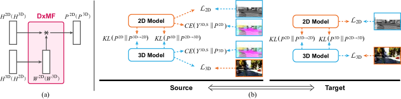
Figure 3: (a) The details of our DxMF. The thick arrow corresponds to the modality in which the features generate dynamic weights. (b) The supervision of the source and the target domain. Mx2M introduces the cross-modal self-supervision on the target domain, which non-exists in previous methods.

As for the information flow, we illustrate it in Fig.3(b). The whole network is alternately trained on the source and the target domain. When the models are trained on the source domain, all six heads work. The heads for xMRP are respectively self-supervised by the origin image/point. The two DxMF heads that predict the segmentation results are both supervised by $Y^{\rm{3D,S}}$. The two mimicking heads are internally supervised by the outputs from the cross-modal DxMF heads (e.g. $P^{\rm{3D\rightarrow 2D}}$ supervised by $P^{\rm{2D}}$). When the models are trained on the target domain, the DxMFs heads cannot be supervised because of lacking annotations. The other heads normally work as above. The loss functions of segmentation and mimicking heads are the same as previous methods (Jaritz et al. 2020; Peng et al. 2021; Liu et al. 2021a) for convenience, where the positions are like in Fig.3(b). The $CE(\cdot)$ and $KL(\cdot)$ are loss functions of cross-entropy and KL divergence, respectively.

3.2 xMRP

The core solution of the Mx2M, xMRP, removes a portion of the data in one modality and learns to predict the full content in the other one, which is related but different from the core solution in masked single-modality modeling. As the name implies, this procedure is divided into two steps. For the step of removal, we randomly select some patches of the image/points and mask them inspired by the way in MAE (He et al. 2022). Considering that 3D points are hard to mask by patches, we first project them into the image. We use two hyper-parameters to control the masking proceeding: the $p$ indicating the size of each patch, and the $mr$ representing the masking ratio of the whole image/points (i.e. masking $mr$ of all patches). The $mr$ cannot be as high as that in (Bao, Dong, and Wei 2022; He et al. 2022) because the CNN backbone in our method cannot perform well if the shape of objects is highly destroyed (Geirhos, Meding, and Wichmann 2020). Besides, due to our segmentation task, the inputs cannot always be masked and at least one modality is complete to guarantee the existence of full semantics. Thus we use another two hyper-parameters to define the ratio when masking each modality: $m_{\rm{2D}}$ meaning the ratio when masking 2D and $m_{\rm{3D}}$ indicating when masking 3D (i.e. masking images at times of $m_{\rm{2D}}$, masking points on times of $m_{\rm{3D}}$, and no masking when (1-$m_{\rm{2D}}$-$m_{\rm{3D}}$)). We can control the inputs by ($p,mr,m_{\rm{2D}},m_{\rm{3D}}$) to make the model adapt to different DA scenarios. As is shown in Fig.2, $X^{\rm{2D}}$ and $X^{\rm{3D}}$ processed by these hyper-parameters (denoted as the new $X^{\rm{2D}}$ and $X^{\rm{3D}}$) are sent into the networks as inputs.

The next step is the cross-modal prediction that provides self-supervision. Inspired by the conclusion in (Wang et al. 2021) about the good effect of MLP on unsupervised tasks, we use the same MLP heads with middle channels of 4096 for both 2D and 3D to generate the results $M^{\rm{2D}\rightarrow{3D}}$ and $M^{\rm{3D}\rightarrow{2D}}$ for 3D and 2D, respectively. Motivated by (He et al. 2022), the losses are correspondingly calculated as follows:

$$\mathcal{L}_{2D}=L_{2}(\widehat{X}^{\rm{3D}}||M^{\rm{2D}\rightarrow{3D}}),\ \ {\rm and}\ \mathcal{L}_{3D}=L_{2}(\widehat{X}^{\rm{2D}}||M^{\rm{3D}\rightarrow{2D}}).$$ (1)

The $\widehat{X}^{\rm{3D}}$ means the original 3D point clouds. The $\widehat{X}^{\rm{2D}}$ indicates the sampled pixels when $\widehat{X}^{\rm{3D}}$ projects into the original image. $L_{2}(\cdot)$ signs the mean squared error. It is noteworthy that we predict the full contents rather than the removed ones in masked single-modality modeling. The model can learn more 2D-3D correspondences from non-masked parts because the masked modality is different from the predicted one, which is not available in methods of masked single-modality modeling.

Herein we finish the core proceeding of our Mx2M. The ($p,mr,m_{\rm{2D}},m_{\rm{3D}}$) are set as (16, 0.15, 0.2, 0.2), (4, 0.3, 0.1, 0.3), and (4, 0.25, 0.3, 0.1) for scenarios of USA/Singapore, Day/Night, and A2D2/SemanticKITTI, respectively. The experiments for USA/Singapore are reported in Sec.4.2 and the other two are in Appendix.A. Our network can learn sufficient 2D-3D correspondences on different DA scenarios in this way, which fixes the lacking of supervision and then reduces the domain gap.

3.3 DxMF

The whole network can learn more complementarity between modalities by feature matching, so it is still important for our Mx2M. Inspired by SOLO V2 (Wang et al. 2020b) which gains great progress compared with SOLO (Wang et al. 2020a) via kernel-feature correspondences by locations, our DxMF constructs cross-modal kernel-feature correspondences for feature matching. The pipeline is shown in Fig.3(a). Compared with simple final linear layers in xMUDA (Jaritz et al. 2020), we use dynamic filters to segment the results. We make the procedure of segmenting the 2D results as an example to illustrate our DxMF and so do on 3D. The kernel weights $W^{\rm{2D}}\in\mathbb{R}^{\rm{N}\times F^{\rm{2D}}\times\rm{C}}$ of the filter for 2D segmentation are generated from 3D features $H^{\rm{3D}}$ by a linear layer (similarly, $W^{\rm{3D}}\in\mathbb{R}^{\rm{N}\times F^{\rm{3D}}\times\rm{C}}$ from $H^{\rm{2D}}$). As the 2D features $H^{\rm{2D}}$ have a spatial size of ($\rm{N},F^{\rm{2D}}$), the result of one point is got:

$$P^{\rm{2D}}_{i}=W^{\rm{2D}}_{i}\ast H^{\rm{2D}}_{i},\ \ {\rm where}\ \ i\in\rm{N}.$$ (2)

The $\ast$ indicates the dynamic convolution. We can get the segmentation results $P^{\rm{2D}}$ after all the $P^{\rm{2D}}_{i}$ joined together. As we dynamically construct the 2D-3D correspondences for feature matching, by which the model learns more suitable complementarity compared with the ways in previous methods (Jaritz et al. 2020; Peng et al. 2021). We provide experiments on this comparison and ones on the scheme of the dynamic feature matching about other heads, where the results are shown in Sec.4.2.

$p$	4	8	16	32
2D	60.0	60.3	60.4	60.1
3D	53.4	53.6	53.8	53.2

(a) $mr$, $m_{\rm{2D}}$, and $m_{\rm{3D}}$ are fixed.

$mr$	0.15	0.20	0.25	0.10
2D	60.4	60.1	60.3	60.0
3D	53.8	53.8	53.0	53.2

(b) $p$=16, $m_{\rm{2D}}$ and $m_{\rm{3D}}$ are fixed.

Head	Linear	MLP	2 MLPs
2D	61.4	62.0	61.5
3D	56.5	57.6	57.4

(c) ($p$, $mr$, $m_{\rm{2D}}$, $m_{\rm{3D}}$)=(16, 0.15, 0.2, 0.2).

Table 1: Ablation studies for $p$, $mr$, and different heads for prediction correspondingly in (a), (b) and (c).

	0.1	0.2	0.3	0.4	0.5	0.6	0.7
0.1	(60.4, 53.8)	(60.9, 54.1)	(61.2, 52.4)	(61.5, 52.1)	(60.5, 52.3)	(59.8, 51.6)	(59.7, 51.1)
0.2	(60.5, 55.1)	(61.4, 56.5)	(59.4, 54.3)	(59.0, 53.9)	(58.9, 54.1)	(58.2, 52.9)	-
0.3	(60.2, 54.2)	(60.0, 57.6)	(59.0, 52.7)	(58.5, 52.6)	(57.7, 51.8)	-	-
0.4	(59.5, 53.5)	(58.6, 54.1)	(57.9, 52.8)	(56.7, 51.7)	-	-	-
0.5	(58.6, 52.0)	(57.3, 51.9)	(57.2, 50.6)	-	-	-	-
0.6	(58.0, 51.2)	(57.5, 51.0)	-	-	-	-	-
0.7	(57.4, 50.1)	-	-	-	-	-	-

Table 2: Ablation for $m_{\rm{2D}}$ and $m_{\rm{3D}}$ with $p$=16 and $mr$=0.15. (mIoU 2D, mIoU 3D) correspondingly denote results for 2D and 3D networks, which are balance when $m_{\rm{2D}}$=0.2 and $m_{\rm{3D}}$=0.2.

4 Experiments

4.1 Implementation Details

Datasets.

We follow three real-to-real adaptation scenarios in xMUDA (Jaritz et al. 2020) to implement our method, the settings of which include country-to-country, day-to-night, and dataset-to-dataset. The gaps between them raise. Three autonomous driving datasets are chosen, including nuScenes (Caesar et al. 2020), A2D2 (Geyer et al. 2019), and SemanticKITTI (Behley et al. 2019), where LiDAR and camera are synchronized and calibrated. In this way, we can compute the projection between a 3D point and the corresponding 2D pixel. We only utilize the 3D annotations for segmentation. In nuScenes, a point falling into a 3D bounding box is assigned the label corresponding to the object, as the dataset only contains labels for the 3D box rather than the segmentation. The nuScenes is leveraged to generate splits Day/Night and USA/Singapore, which correspond to day-to-night and country-to-country adaptation. The other two datasets are used for A2D2/SemanticKITTI ( i.e. dataset-to-dataset adaptation), where the classes are modified as 10 according to the alignments in (Jaritz et al. 2020).

Metrics.

Like other segmentation works, the mean intersection over union (mIoU) is adopted as the metric for evaluating the performance of the models (both 2D and 3D) for all datasets. In addition, we follow the new mIoU calculating way in (Jaritz et al. 2020), which jointly considers both modalities and is obtained by taking the mean of the predicted 2D and 3D probabilities after softmax (denoted as ’Avg mIoU’).

Inputs & Labels.

For easily conducting masked modeling, we resize images into the sizes that could be divisible by $p$. The images in nuScenes (i.e. Day/Night and USA/Singapore) are resized as 400$\times$224, whereas the ones in A2D2 and SemanticKITTI are reshaped as 480$\times$304. All images are normalized and then become the inputs/labels of the 2D/3D network. As for points, a voxel size of 5cm is adopted for the 3D network, which is small enough and ensures that only one 3D point lies in a voxel. The coordinates of these voxels are adopted as the labels for the 2D network.

Training.

We use the PyTorch 1.7.1 framework on an NVIDIA Tesla V100 GPU card with 32GB RAM under CUDA 11.0 and cuDNN 8.0.5. For nuScenes, the mini-batch Adam (Kingma and Ba 2015) is configured as the batch size of 8, $\beta_{1}$ of 0.9, and $\beta_{2}$ of 0.999. All models are trained for 100k iterations with the initial learning rate of 1e-3, which is then divided by 10 at the 80k and again at the 90k iteration. For the A2D2/SemanticKITTI, the batch size is set as 4, while related models are trained for 200k and so do on other configurations, which is caused by the limited memory. The models with ’+PL’ share the above proceeding, where segmentation heads are extra supervised with pseudo labels for the target dataset. As for these pseudo labels, we strictly follow the ways in (Jaritz et al. 2020) to prevent manual supervision, i.e. using the last checkpoints of models without PL to generate them offline.

4.2 Ablation Studies

To define the effectiveness of each component, we conduct ablation studies on them, respectively. As xMUDA (Jaritz et al. 2020) is the first method of cross-modal DA in 3D segmentation and is the baseline of all related methods (Liu et al. 2021a; Peng et al. 2021), we continue this habit and choose xMUDA as our baseline. By default, all results are reported based on the USA/Singapore scenario. For a fair comparison, we train models with each setting for 100k iterations with a batch size of 8. We also provide experiments on other scenarios, which are reported in Sec.6.

Strategy	2D	3D
xMRP	62.0	57.6
2D+3D	59.4	53.3
only 3D	58.9	52.6
only 2D	57.9	51.9

(a) Strategies of removal-prediction.

Setting	2D	3D
-	62.0	57.6
+DxMF	64.1	64.2
+DsCML (Peng et al. 2021)	58.0	50.6
DsCML† (Peng et al. 2021)	57.8	50.2
DsCML (Peng et al. 2021)	61.3	53.3

(b) Settings of cross-modal feature matching.

Setting	2D	3D
DxMF on Prediction	64.1	64.2
DxMF on Prediction (w/o xMRP)	61.1	53.9
DxMF on Mimicking	59.4	52.4
DxMF on xMRP	55.4	50.8

(c) DxMF on three output heads.

Table 3: Ablation for removal-prediction and DxMF in (a), (b) and (c). Three heads in (c) are mentioned in Sec.3.1.

Modality	Method	USA/Singapore			Day/Night			A2D2/SemanticKITTI
		2D	3D	Avg	2D	3D	Avg	2D	3D	Avg
	Backbones(source only)	53.4	46.5	61.3	42.2	41.2	47.8	36.0	36.6	41.8
	Backbones(on target)	66.4	63.8	71.6	48.6	47.1	55.2	58.3	71.0	73.7
Uni-modal	MinEnt (Vu et al. 2019)	53.4	47.0	59.7	44.9	43.5	51.3	38.8	38.0	42.7
	Deep logCORAL (Morerio, Cavazza, and Murino 2018)	52.6	47.1	59.1	41.4	42.8	51.8	35.8	39.3	40.3
	PL (Li, Yuan, and Vasconcelos 2019)	55.5	51.8	61.5	43.7	45.1	48.6	37.4	44.8	47.7
	FCNs in the Wild (Hoffman et al. 2016)	53.7	46.8	61.0	42.6	42.3	47.9	37.1	43.5	43.6
	CyCADA (Hoffman et al. 2018)	54.9	48.7	61.4	45.7	45.2	49.7	38.2	43.9	43.9
	AdaptSegNet (Tsai et al. 2018)	56.3	47.7	61.8	45.3	44.6	49.6	38.8	44.3	44.2
	CLAN (Luo et al. 2019)	57.8	51.2	62.5	45.6	43.7	49.2	39.2	44.7	44.5
Cross-modal	xMUDA (Jaritz et al. 2020)	59.3	52.0	62.7	46.2	44.2	50.0	36.8	43.3	42.9
	xMUDA+PL (Jaritz et al. 2020)	61.1	54.1	63.2	47.1	46.7	50.8	43.7	48.5	49.1
	AUDA (Liu et al. 2021a)	59.8	52.0	63.1	49.0	47.6	54.2	43.0	43.6	46.8
	AUDA+PL (Liu et al. 2021a)	61.9	54.8	65.6	50.3	49.7	52.6	46.8	48.1	50.6
	DsCML (Peng et al. 2021)	61.3	53.3	63.6	48.0	45.7	51.0	39.6	45.1	44.5
	DsCML+CMAL (Peng et al. 2021)	63.4	55.6	64.8	49.5	48.2	52.7	46.3	50.7	51.0
	DsCML+CMAL+PL (Peng et al. 2021)	63.9	56.3	65.1	50.1	48.7	53.0	46.8	51.8	52.4
	Mx2M	64.1	64.2	64.2	49.7	49.9	49.8	44.6	48.2	47.1
	Mx2M+PL	67.4	67.5	67.4	52.4	56.3	54.6	48.6	53.0	51.3

Table 4: Comparison results with both uni-modal and multi-modal adaptation methods for 3D semantic segmentation. Our Mx2M achieves state-of-the-art performance on most metrics.

Ablation on xMRP

As mentioned in Sec.3.2, in xMRP, we use four hyper-parameters ($p,mr,m_{\rm{2D}},m_{\rm{3D}}$) to control the proceeding of masking inputs and two heads of MLP to predict the cross-modality. To validate the effectiveness of the masked cross-modality modeling strategy, we insert simple xMRPs into xMUDA. The (4, 0.15, 0.1, 0.1) are selected as the start point because of the low mask ratio and the low masking 2D/3D ratio, which are suitable for the task of segmentation. As for heads, we start from the simplest linear layers. The mIoU for (2D, 3D) in this setting are (60.0, 53.4), which are better than the segmentation results of (59.3, 52.0) in xMUDA. The good results demonstrate the significance of masked cross-modality modeling. We next explore the effectiveness of detailed settings.

Ablation on Hyper-parameters.

To determine the suitable input settings for the current scenario, we conduct ablation studies on ($p,mr,m_{\rm{2D}},m_{\rm{3D}}$), respectively. We start from (4, 0.15, 0.1, 0.1) and first confirm $p$ with fixed other numbers, where the mIoU of 2D and 3D are shown in Tab.1(a). The networks gain the best metrics at $p=16$. The next job is to define $mr$, the results of which are illustrated in Tab.1(b). Both metrics decrease with the raising of $mr$, but when $mr=0.10$ so do results. Hence the models have the best results when $mr=0.15$. Finally, we determine the $m_{\rm{2D}}$ and $m_{\rm{3D}}$. As mentioned in Sec.3.2, $(1-m_{\rm{2D}}$-$m_{\rm{3D}})>0$ because of keeping the full semantics. We design plenty of combinations for these two hyper-parameters, where the details are shown in Tab.2. The metrics are not good when $m_{\rm{2D}}$ and $m_{\rm{3D}}$ are too large, which matches the fact that our CNN backbones cannot integrate a high mask ratio like (He et al. 2022). We get results of (61.4, 56.5) with suitable $m_{\rm{2D}}=0.2$ and $m_{\rm{3D}}=0.2$, and then appropriate hyper-parameters (16, 0.15, 0.2, 0.2) for the scenario.

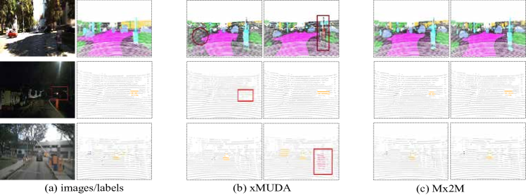
Figure 4: Comparison of visual results on three scenarios. The images/points from the top row to the bottom come from the A2D2/SemanticKITTI, Day/Night, and USA/Singapore scenarios, respectively. With the joining of masked cross-modality modeling, errors caused by the domain gap are reduced. Best view it on screen.

Ablation for Removal and Prediction.

We obtain the results of (61.4, 56.5) with the simple linear layer. According to the conclusion in (Wang et al. 2021), the network performs well when having an MLP layer. Therefore we compare the schemes of linear layer, a single MLP with mid channels of 4096, and two same MLPs with the 4096 mid channels. They are used to predict both modalities, where the results are shown in Tab.1(c). A single MLP also does for our DA task. Besides, some other removal-prediction strategies are also attempted besides the cross-modal one. We illustrate the segmentation metrics in Tab.3(a). We have tried respectively removing and predicting the content in single-modality (denoted as ’2D+3D’), only in 3D point clouds, and only in 2D images. Here only removed portions are set as labels. We can see ’2D+3D’ has similar results as xMUDA (Jaritz et al. 2020), because only rare patches work and bring about seldom information in this scheme. Similarly, the cross-modal scheme performs well thanks to 2D-3D correspondences from all contents, which is beneficial to this task (Peng et al. 2021; Li, Yuan, and Vasconcelos 2019). Finally, we gain the (+2.0, +4.2) increase with our xMRP for 2D and 3D performance, respectively.

Ablation on DxMF

All above experiments are based on the same way of feature matching as xMUDA (Jaritz et al. 2020), where the segmentation results are got based on two linear layers. We also conduct experiments on our DxMF, which achieves cross-modal feature matching and then the segmentation by dynamically constructing kernel-feature correspondences. The comparison is shown in the first two rows of Tab.3(b), our DxMF performs the better 2D-3D complementarity and especially increases the 3D performance. We also try to combine the means of sparse-to-dense cross-modal feature matching, DsCML (Peng et al. 2021), with the masked cross-modality modeling, where the metrics are illustrated in the last three rows in Tab.3(c). The results with ’${\dagger}$’ or not denote that they are from the implementation of the official source code or from the paper. As our experiments are based on the official source code, we still gain the increase with the join of xMRP. In all, the good metrics prove the effectiveness of our DxMF.

We also validate the results for only using DxMF, which is reported in the first two rows of Tab.3(c). Besides, our Mx2M has three output heads for each modality according to Sec.3.1. We also conduct experiments on DxMF on them besides the above experiments on prediction heads. Like adding DxMF to prediction heads, we add DxMF to other ones on both modalities. The results are reported in Tab.3(c). Both mimicking heads and ones for xMRP do not match the DxMF. We may infer that the former is not involved in segmentation and the latter is like respective single-modal prediction in Tab.3(a). Both situations are not suitable for our DxMF. After all experiments, our Mx2M outperforms the Baseline xMUDA (+4.8, +12.2) for 2D and 3D in total, which shows that the Mx2M does work.

4.3 Limitations

Considering previous works (Liu et al. 2021a; Peng et al. 2021) attempt to introduce the adversarial learning (AL) into the DA in 3D semantic segmentation, we also add the extra heads for AL in both 2D and 3D. We use the simple AL in AUDA (Liu et al. 2021a) and the CMAL in DsCML (Peng et al. 2021). The results for 2D and 3D are not ideal, which are correspondingly (56.26, 51.76) and (49.75, 41.94) for AL in AUDA and CMAL. Compared with the metrics of (64.1, 64.2) in the scheme without AL, they decrease so much. We think it is the limitation in our Mx2M that our method does not match AL.

4.4 Comparison with The State-of-the-art

We evaluate our Mx2M on the above three real-to-real DA scenarios and compare the results with some methods. First, we train the backbones on source only and on target only (except on the Day/Night, where the batches of 50%/50% Day/Night are used to prevent overfitting). The two results can be seen as the upper and the lower limit of the DA effectiveness. Next, some representative uni-modal DA methods are compared. These uni-modal methods are correspondingly evaluated on U-Net with ResNet-34 for 2D and SparseConvNet for 3D, which are the same as our backbones. We use the results from (Peng et al. 2021) for convenience. Finally, We also compare our method with some cross-modal methods, including xMUDA (Jaritz et al. 2020), AUDA (Liu et al. 2021a), and DsCML (Peng et al. 2021). These cross-modal methods and our Mx2M are also trained with the data with pseudo labels on the target domain, where the proceeding can be seen in Sec.4.1.

All comparison results for 3D segmentation are reported in Tab.4. We can see that the Mx2M gains the (2D mIoU, 3D mIoU) on average of (+5.4, +7.6) compared with the baseline xMUDA, which proves the DA performance of our method. Specifically, for the USA/Singapore scenario, the bare Mx2M even surpasses xMUDA with PL. In Day/Night, though the metric without PL looks normal, the result with PL shows a surprising increase that is close to the upper limit. As for the A2D2/SemanticKITTI, the Mx2M outperforms all methods on 2D and 3D metrics with a 0.9 less Avg mIoU compared to the DsCML. In total, our Mx2M gains state-of-the-art performance on most metrics. We also provide some visual results, which are shown in Fig.4. More visual results can be seen in Sec.7.

5 Conclusion

In this paper, we propose a method named Mx2M for domain adaptation in 3D semantic segmentation, which utilizes masked cross-modality modeling to solve the problem of lacking supervision on the target domain and then reduce the large gap. The Mx2M includes two components. The core solution xMRP makes the Mx2M adapts to various scenarios and provides cross-modal self-supervision. A new way of cross-modal feature matching named DxMF ensures that the whole method exploits more suitable 2D-3D complementarity and then segments results. We achieve state-of-the-art performance on three DA scenarios for 3D segmentation, including USA/Singapore, Day/Night, and A2D2/SemanticKITTI. Specifically, the Mx2M with pseudo labels achieves the (2D mIoU, 3D mIoU, Avg mIoU) of (67.4, 67.5, 67.4), (52.4, 56.3, 54.6), and (48.6, 53.0, 51.3) for the three scenarios. All the above results demonstrate the effectiveness of our method.

6 Ablation Studies on Scenarios of Day/Night and A2D2/SemanticKITTI

We also conduct ablation studies on the scenarios of Day/Night and A2D2/SemanticKITTI. Similarly, the xMUDA (Jaritz et al. 2020) is also selected as the backbone. We train the models with each Day/Night setting for 100k iterations with a batch size of 8 and with each A2D2/SemanticKITTI setting for 200k iterations with a batch size of 4 because of limited resources. The proceedings are basically as those in USA/Singapore and as follows.

6.1 Ablations on Day/Night

We first validate the effectiveness of the masked cross-modality modeling strategy. The four hyper-parameters ($p,mr,m_{\rm{2D}},m_{\rm{3D}}$) are set as (4, 0.15, 0.1, 0.1), which is the same as what we do for the USA/Singapore and for the same reason in Sec.4.2.1 of the body. As for the heads for predicting segmentation, we start from the simplest linear layers. The mIoU results for (2D, 3D) are (47.3, 45.9), which are better than the segmentation indexes of (46.2, 44.2) in our baseline xMUDA. The good results demonstrate the significance of the strategy for masked cross-modality modeling. We next explore the effectiveness of detailed settings.

To determine the suitable input settings for the current scenario, we conduct ablation studies on ($p,mr,m_{\rm{2D}},m_{\rm{3D}}$), respectively. We start from (4, 0.15, 0.1, 0.1) and first confirm $p$ with fixed other numbers, where the mIoU of 2D and 3D are shown in Tab.5(a). The start point is the most suitable one for this scenario, i.e. $p=4$. The next job is to define $mr$, the results of which are illustrated in Tab.5(b). The models have the best results when $mr=0.3$. Finally, we determine the $m_{\rm{2D}}$ and $m_{\rm{3D}}$. We design plenty of combinations for these two hyper-parameters, where the details are shown in Tab.6. We get results of (48.9, 48.5) with suitable numbers, where $m_{\rm{2D}}=0.1$ and $m_{\rm{3D}}=0.3$, and then appropriate hyper-parameters (4, 0.3, 0.1, 0.3) for the scenario.

We obtain the results of (48.9, 48.5) with the simple linear layer. According to the conclusion in (Wang et al. 2021), the network performs well when having an MLP layer. Therefore we compare the schemes of linear layer, a single MLP with mid channels of 4096, and two same MLPs with the 4096 mid channels. They are used to predict both modalities, where the results are shown in Tab.5(c). A single MLP also does for our DA task. Finally, the DxMF is added to the Mx2M, the results of which are illustrated in Tab.5(d). With the join of the DxMF, we gain the mIoU of (49.7, 49.9) for the scenario of Day/Night.

6.2 Ablations on A2D2/SemanticKITTI

The proceeding of ablation studies on A2D2/SemanticKITTI is the same as what in Day/Night. First, the effectiveness of the masked cross-modality modeling strategy is validated. Our results are (37.9, 44.3) v.s. (36.8, 43.3) of the ones in xMUDA (Jaritz et al. 2020). Next, we determine four hyper-parameters ($p,mr,m_{\rm{2D}},m_{\rm{3D}}$), where the procedure is the same as the above. We report them in Tab.7(a), Tab.7(b), and Tab.8, respectively. They are set as (4, 0.25, 0.3, 0.1) for the A2D2/SemanticKITTI scenario. We then define the prediction heads with results (41.5, 46.2), which is shown in Tab.7(c). The MLP works again. Finally, we validate the effectiveness of the DxMF, the results of which are illustrated in Tab.7(d). We gain the mIoU of (44.6, 48.2) for the A2D2/SemanticKITTI.

7 More Visual Results on the Mx2M

As is mentioned in Sec.4.4 of the main body, we offer more visual results in Fig.5. The images/points from the top row to the bottom correspondingly come from the A2D2/SemanticKITTI, USA/Singapore, and Day/Night scenarios, where every three rows belong to the same scenario. Our Mx2M has a balanced performance in all three scenarios.

$p$	4	8	2
2D	47.3	47.2	46.6
3D	45.9	45.2	45.8

(a) $mr$, $m_{\rm{2D}}$, and $m_{\rm{3D}}$ are fixed.

$mr$	0.15	0.20	0.25	0.30	0.35
2D	47.3	47.2	47.6	47.9	47.2
3D	45.9	46.1	46.2	46.5	46.3

(b) $p=4$, $m_{\rm{2D}}$ and $m_{\rm{3D}}$ are fixed.

Head	Linear	MLP	2 MLPs
2D	48.9	49.5	49.3
3D	48.5	49.3	48.9

(c) ($p$, $mr$, $m_{\rm{2D}}$, $m_{\rm{3D}}$)=(4, 0.3, 0.1, 0.3).

Setting	2D	3D
-	49.5	49.3
+DxMF	49.7	49.9

(d) Ablation for DxMF.

Table 5: Ablation studies for $p$, $mr$, different heads, and DxMF about Day/Night for prediction correspondingly in (a), (b), (c) and (d).

	0.1	0.2	0.3	0.4	0.5	0.6	0.7
0.1	(47.9, 46.5)	(48.0, 46.6)	(48.6, 47.1)	(48.3, 47.5)	(47.8, 47.9)	(47.2, 46.9)	(47.6, 46.7)
0.2	(48.5, 47.9)	(48.8, 48.0)	(48.8, 48.4)	(48.4, 46.7)	(47.7, 47.5)	(46.8, 46.6)	-
0.3	(48.9, 48.5)	(48.6, 47.9)	(48.3, 46.7)	(47.6, 47.9)	(48.3, 45.2)	-	-
0.4	(48.8, 48.1)	(47.5, 46.8)	(47.8, 45.2)	(47.9, 47.0)	-	-	-
0.5	(47.1, 48.4)	(47.0, 46.5)	(48.0, 43.9)	-	-	-	-
0.6	(47.2, 48.5)	(46.0, 46.7)	-	-	-	-	-
0.7	(46.6, 48.3)	-	-	-	-	-	-

Table 6: Ablation for $m_{\rm{2D}}$ and $m_{\rm{3D}}$ with $p=4$ and $mr=0.3$ in the Day/Night. (mIoU 2D, mIoU 3D) denote results of corresponding networks, which are better when $m_{\rm{2D}}=0.1$ and $m_{\rm{3D}}=0.3$.

$p$	4	8	2
2D	37.9	37.1	37.4
3D	44.3	43.6	43.2

(a) Ablation for $p$ with fixed $mr$, $m_{\rm{2D}}$.

$mr$	0.15	0.20	0.25	0.30
2D	37.9	38.3	39.1	38.0
3D	44.3	44.4	45.0	44.0

(b) Ablation for $mr$ with $p=4$ and fixed $m_{\rm{2D}}$ as well as $m_{\rm{3D}}$.

Head	Linear	MLP	2 MLPs
2D	41.5	43.6	43.0
3D	46.2	47.8	46.8

(c) Ablation on different heads for prediction.

Setting	2D	3D
-	43.6	47.8
+DxMF	44.6	48.2

(d) Ablation for DxMF.

Table 7: Ablation studies for $p$, $mr$, different heads, and DxMF about A2D2/SemanticKITTI for prediction correspondingly in (a), (b), (c) and (d)..

	0.1	0.2	0.3	0.4	0.5	0.6	0.7
0.1	(39.1, 45.0)	(40.2, 45.5)	(41.5, 46.2)	(40.9, 45.5)	(40.4, 45.3)	(40.3, 44.9)	(39.2, 45.4)
0.2	(35.6, 42.8)	(40.3, 44.1)	(40.8, 44.9)	(39.8, 45.1)	(39.6, 45.0)	(40.4, 40.3)	-
0.3	(35.3, 45.6)	(40.8, 43.4)	(39.9, 44.4)	(39.1, 43.4)	(39.7, 41.6)	-	-
0.4	(37.0, 41.8)	(39.9, 44.3)	(38.1, 43.0)	(37.4, 44.9)	-	-	-
0.5	(40.3, 45.5)	(39.1, 45.2)	(39.0, 42.9)	-	-	-	-
0.6	(37.1, 45.5)	(37.3, 44.4)	-	-	-	-	-
0.7	(36.7, 44.8)	-	-	-	-	-	-

Table 8: Ablation for $m_{\rm{2D}}$ and $m_{\rm{3D}}$ with $p=4$ and $mr=0.25$ in the A2D2/SemanticKITTI. (mIoU 2D, mIoU 3D) denote results of corresponding networks, which are better when $m_{\rm{2D}}=0.3$ and $m_{\rm{3D}}=0.1$.

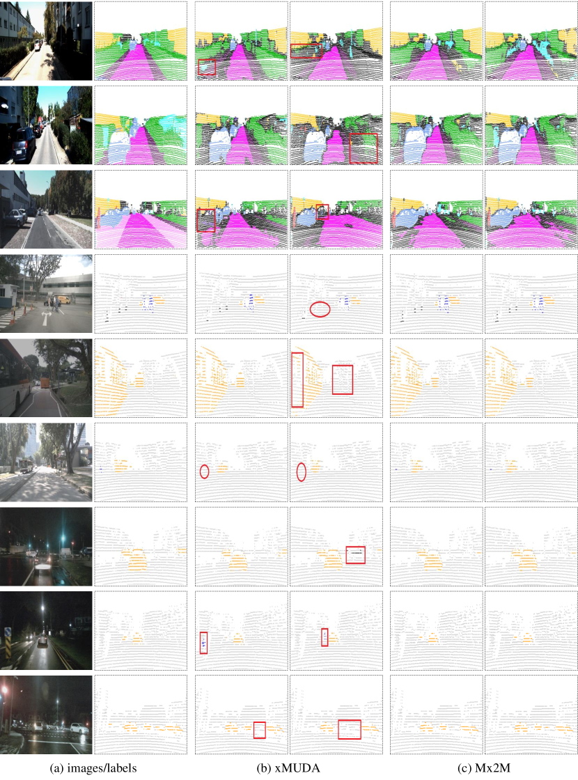
Figure 5: Comparison of visual results on three scenarios. Our Mx2M achieves better domain adaptation and more precise segmentation.

References

- Baevski et al. (2020) Baevski, A.; Zhou, Y.; Mohamed, A.; and Auli, M. 2020. wav2vec 2.0: A framework for self-supervised learning of speech representations. NeurIPS, 33: 12449–12460.
- Bao, Dong, and Wei (2022) Bao, H.; Dong, L.; and Wei, F. 2022. Beit: Bert pre-training of image transformers. In ICLR.
- Behley et al. (2019) Behley, J.; Garbade, M.; Milioto, A.; Quenzel, J.; Behnke, S.; Stachniss, C.; and Gall, J. 2019. Semantickitti: A dataset for semantic scene understanding of lidar sequences. In ICCV, 9297–9307.
- Caesar et al. (2020) Caesar, H.; Bankiti, V.; Lang, A. H.; Vora, S.; Liong, V. E.; Xu, Q.; Krishnan, A.; Pan, Y.; Baldan, G.; and Beijbom, O. 2020. nuscenes: A multimodal dataset for autonomous driving. In CVPR, 11621–11631.
- Carreira and Zisserman (2017) Carreira, J.; and Zisserman, A. 2017. Quo vadis, action recognition? a new model and the kinetics dataset. In CVPR, 6299–6308.
- Dai and Nießner (2018) Dai, A.; and Nießner, M. 2018. 3dmv: Joint 3d-multi-view prediction for 3d semantic scene segmentation. In ECCV, 452–468.
- Deng et al. (2009) Deng, J.; Dong, W.; Socher, R.; Li, L.-J.; Li, K.; and Fei-Fei, L. 2009. Imagenet: A large-scale hierarchical image database. In CVPR, 248–255.
- Fu et al. (2021) Fu, T.-J.; Li, L.; Gan, Z.; Lin, K.; Wang, W. Y.; Wang, L.; and Liu, Z. 2021. VIOLET: End-to-End Video-Language Transformers with Masked Visual-token Modeling. arXiv preprint arXiv:2111.12681.
- Gao and Grauman (2021) Gao, R.; and Grauman, K. 2021. Visualvoice: Audio-visual speech separation with cross-modal consistency. In CVPR, 15490–15500. IEEE.
- Geirhos, Meding, and Wichmann (2020) Geirhos, R.; Meding, K.; and Wichmann, F. A. 2020. Beyond accuracy: quantifying trial-by-trial behaviour of CNNs and humans by measuring error consistency. NeurIPS, 33: 13890–13902.
- Genova et al. (2021) Genova, K.; Yin, X.; Kundu, A.; Pantofaru, C.; Cole, F.; Sud, A.; Brewington, B.; Shucker, B.; and Funkhouser, T. 2021. Learning 3D Semantic Segmentation with only 2D Image Supervision. In 3DV, 361–372. IEEE.
- Geyer et al. (2019) Geyer, J.; Kassahun, Y.; Mahmudi, M.; Ricou, X.; Durgesh, R.; S. Chung, A.; Hauswald, L.; Hoang Pham, V.; Mühlegg, M.; Dorn, S.; Fernandez, T.; Jänicke, M.; Mirashi, S.; Savani, C.; Sturm, M.; Vorobiov, O.; and Schuberth, P. 2019. A2D2: AEV autonomous driving dataset. http://www.a2d2.audi/.
- Graham, Engelcke, and Van Der Maaten (2018) Graham, B.; Engelcke, M.; and Van Der Maaten, L. 2018. 3d semantic segmentation with submanifold sparse convolutional networks. In CVPR, 9224–9232.
- He et al. (2022) He, K.; Chen, X.; Xie, S.; Li, Y.; Dollár, P.; and Girshick, R. 2022. Masked Autoencoders Are Scalable Vision Learners. CVPR.
- He et al. (2016) He, K.; Zhang, X.; Ren, S.; and Sun, J. 2016. Deep Residual Learning for Image Recognition. In CVPR, 770–778.
- Hoffman et al. (2018) Hoffman, J.; Tzeng, E.; Park, T.; Zhu, J.-Y.; Isola, P.; Saenko, K.; Efros, A.; and Darrell, T. 2018. Cycada: Cycle-consistent adversarial domain adaptation. In ICML, 1989–1998. PMLR.
- Hoffman et al. (2016) Hoffman, J.; Wang, D.; Yu, F.; and Darrell, T. 2016. Fcns in the wild: Pixel-level adversarial and constraint-based adaptation. arXiv preprint arXiv:1612.02649.
- Hu et al. (2021) Hu, W.; Zhao, H.; Jiang, L.; Jia, J.; and Wong, T.-T. 2021. Bidirectional projection network for cross dimension scene understanding. In CVPR, 14373–14382.
- Jaritz et al. (2020) Jaritz, M.; Vu, T.-H.; Charette, R. d.; Wirbel, E.; and Pérez, P. 2020. xmuda: Cross-modal Unsupervised Domain Adaptation for 3d Semantic Segmentation. In CVPR, 12605–12614.
- Jing, Zhang, and Tian (2021) Jing, L.; Zhang, L.; and Tian, Y. 2021. Self-supervised feature learning by cross-modality and cross-view correspondences. In CVPRW, 1581–1591.
- Kenton and Toutanova (2019) Kenton, J. D. M.-W. C.; and Toutanova, L. K. 2019. BERT: Pre-training of Deep Bidirectional Transformers for Language Understanding. In NAACL-HLT, 4171–4186.
- Kingma and Ba (2015) Kingma, D. P.; and Ba, J. 2015. Adam: A Method for Stochastic Optimization. In ICLR.
- Lee et al. (2021) Lee, J.; Chung, S.-W.; Kim, S.; Kang, H.-G.; and Sohn, K. 2021. Looking into your speech: Learning cross-modal affinity for audio-visual speech separation. In CVPR, 1336–1345.
- Li, Yuan, and Vasconcelos (2019) Li, Y.; Yuan, L.; and Vasconcelos, N. 2019. Bidirectional learning for domain adaptation of semantic segmentation. In CVPR, 6936–6945.
- Liu et al. (2021a) Liu, W.; Luo, Z.; Cai, Y.; Yu, Y.; Ke, Y.; Junior, J. M.; Gonçalves, W. N.; and Li, J. 2021a. Adversarial Unsupervised Domain Adaptation for 3D semantic Segmentation with Multi-modal Learning. ISPRS Journal of Photogrammetry and Remote Sensing, 176: 211–221.
- Liu et al. (2021b) Liu, Y.-C.; Huang, Y.-K.; Chiang, H.-Y.; Su, H.-T.; Liu, Z.-Y.; Chen, C.-T.; Tseng, C.-Y.; and Hsu, W. H. 2021b. Learning from 2D: Contrastive Pixel-to-Point Knowledge Transfer for 3D Pretraining. arXiv preprint arXiv:2104.04687.
- Liu, Qi, and Fu (2021) Liu, Z.; Qi, X.; and Fu, C.-W. 2021. 3D-to-2D distillation for indoor scene parsing. In CVPR, 4464–4474.
- Lu et al. (2021) Lu, K.; Grover, A.; Abbeel, P.; and Mordatch, I. 2021. Pretrained transformers as universal computation engines. arXiv preprint arXiv:2103.05247.
- Luo et al. (2020) Luo, H.; Khoshelham, K.; Fang, L.; and Chen, C. 2020. Unsupervised scene adaptation for semantic segmentation of urban mobile laser scanning point clouds. ISPRS Journal of Photogrammetry and Remote Sensing, 169: 253–267.
- Luo et al. (2019) Luo, Y.; Zheng, L.; Guan, T.; Yu, J.; and Yang, Y. 2019. Taking a closer look at domain shift: Category-level adversaries for semantics consistent domain adaptation. In CVPR, 2507–2516.
- Morerio, Cavazza, and Murino (2018) Morerio, P.; Cavazza, J.; and Murino, V. 2018. Minimal-Entropy Correlation Alignment for Unsupervised Deep Domain Adaptation. In ICLR.
- Peng et al. (2021) Peng, D.; Lei, Y.; Li, W.; Zhang, P.; and Guo, Y. 2021. Sparse-to-dense Feature Matching: Intra and Inter Domain Cross-modal Learning in Domain Adaptation for 3d Semantic Segmentation. In ICCV, 7108–7117.
- Qin et al. (2019) Qin, C.; You, H.; Wang, L.; Kuo, C.-C. J.; and Fu, Y. 2019. Pointdan: A multi-scale 3d domain adaption network for point cloud representation. NeurIPS, 32.
- Radford et al. (2021) Radford, A.; Kim, J. W.; Hallacy, C.; Ramesh, A.; Goh, G.; Agarwal, S.; Sastry, G.; Askell, A.; Mishkin, P.; Clark, J.; et al. 2021. Learning transferable visual models from natural language supervision. In ICML, 8748–8763. PMLR.
- Ronneberger, Fischer, and Brox (2015) Ronneberger, O.; Fischer, P.; and Brox, T. 2015. U-Net: Convolutional Networks for Biomedical Image Segmentation. In MICCAI, 234–241. Springer.
- Shan et al. (2018) Shan, H.; Zhang, Y.; Yang, Q.; Kruger, U.; Kalra, M. K.; Sun, L.; Cong, W.; and Wang, G. 2018. 3-D convolutional encoder-decoder network for low-dose CT via transfer learning from a 2-D trained network. IEEE transactions on medical imaging, 37(6): 1522–1534.
- Tsai et al. (2018) Tsai, Y.-H.; Hung, W.-C.; Schulter, S.; Sohn, K.; Yang, M.-H.; and Chandraker, M. 2018. Learning to adapt structured output space for semantic segmentation. In CVPR, 7472–7481.
- Vu et al. (2019) Vu, T.-H.; Jain, H.; Bucher, M.; Cord, M.; and Pérez, P. 2019. Advent: Adversarial entropy minimization for domain adaptation in semantic segmentation. In CVPR, 2517–2526.
- Wang et al. (2019) Wang, L.; Huang, Y.; Hou, Y.; Zhang, S.; and Shan, J. 2019. Graph attention convolution for point cloud semantic segmentation. In CVPR, 10296–10305.
- Wang et al. (2020a) Wang, X.; Kong, T.; Shen, C.; Jiang, Y.; and Li, L. 2020a. SOLO: Segmenting Objects by Locations. In ECCV.
- Wang et al. (2020b) Wang, X.; Zhang, R.; Kong, T.; Li, L.; and Shen, C. 2020b. SOLOv2: Dynamic and Fast Instance Segmentation. In NeurIPS.
- Wang et al. (2021) Wang, Y.; Tang, S.; Zhu, F.; Bai, L.; Zhao, R.; Qi, D.; and Ouyang, W. 2021. Revisiting the Transferability of Supervised Pretraining: an MLP Perspective. CVPR.
- Wu et al. (2022) Wu, Y.; Li, C.; Bai, J.; Wu, Z.; and Qian, Y. 2022. Time-Domain Audio-Visual Speech Separation on Low Quality Videos. In ICASSP, 256–260. IEEE.
- Xie et al. (2022) Xie, Z.; Zhang, Z.; Cao, Y.; Lin, Y.; Bao, J.; Yao, Z.; Dai, Q.; and Hu, H. 2022. SimMIM: A Simple Framework for Masked Image Modeling. In CVPR.
- Xu et al. (2021) Xu, C.; Yang, S.; Zhai, B.; Wu, B.; Yue, X.; Zhan, W.; Vajda, P.; Keutzer, K.; and Tomizuka, M. 2021. Image2point: 3d point-cloud understanding with pretrained 2d convnets. arXiv preprint arXiv:2106.04180.
- Xu et al. (2022) Xu, H.; Ding, S.; Zhang, X.; Xiong, H.; and Tian, Q. 2022. Masked Autoencoders are Robust Data Augmentors. arXiv preprint arXiv:2206.04846.
- Yu et al. (2022) Yu, X.; Tang, L.; Rao, Y.; Huang, T.; Zhou, J.; and Lu, J. 2022. Point-BERT: Pre-Training 3D Point Cloud Transformers with Masked Point Modeling. In CVPR.
- Zhang et al. (2021) Zhang, B.; Guan, Y.; Liu, H.; Li, W.; and Wang, Y. 2021. DOBNET: Dynamic Object Boundary-Refinement Network for Real-Time Instance Segmentation. In ICME, 1–6.
- Zhang et al. (2020) Zhang, B.; Li, W.; Hui, Y.; Liu, J.; and Guan, Y. 2020. MFENet: Multi-level feature enhancement network for real-time semantic segmentation. Neurocomputing, 393: 54–65.