A threshold model of plastic waste fragmentation: New insights into the distribution of microplastics in the ocean and its evolution over time

Abstract

Plastic pollution in the aquatic environment has been assessed for many years by ocean waste collection expeditions around the globe or by river sampling. While the total amount of plastic produced worldwide is well documented, the amount of plastic found in the ocean, the distribution of particles on its surface and its evolution over time are still the subject of much debate. In this article, we propose a general fragmentation model, postulating the existence of a critical size below which particle fragmentation becomes extremely unlikely. In the frame of this model, an abundance peak appears for sizes around 1mm, in agreement with real environmental data. Using, in addition, a realistic exponential waste feed to the ocean, we discuss the relative impact of fragmentation and feed rates, and the temporal evolution of microplastics (MP) distribution. New conclusions on the temporal trend of MP pollution are drawn.

I Introduction

Plastic waste has been dumped into the environment for nearly 70 years, and more and more data are being collected in order to quantify the extent of this pollution. Under the action of degradation agents (UV, water, stress), plastic breaks down into smaller pieces that gradually invade all marine compartments. If the plastic pollution awareness initially stemmed from the ubiquitous presence of macro-waste, it has now become clear that the most problematic pollution is “invisible” i.e. due to smaller size debris, and the literature exploring microplastics (MP, size between 1 $\mu$m and 5 mm) and nanoplastics (NP, size below 1 $\mu$m) quantities and effects is rapidly increasing. The toxicity of plastic particles being dependent on their sizes and concentrations, it is crucial to know these two parameters in the natural environment to better predict their impacts. While the total amount of plastic produced worldwide is well-documented [1], the total amount of plastic found in the ocean and its time evolution are still under debate: while many repeated surveys and monitoring efforts have failed to demonstrate any convincing temporal trend [2], increasing amounts of plastic are found in some regions, especially in remote areas, and a global increase from ca. 2005 has been suggested [3]. In terms of particle sizes, a lot of efforts have been devoted to collect and accurately identify smaller and smaller MP, leading to the conclusion that MP smaller than ca. 300 $\mu$m were more numerous than larger MP [4, 5, 6].

The purpose and originality of this paper is to explain in a global manner the observed size distribution of particles floating in the oceans. Indeed, this distribution exhibits, in our opinion, some very specific features that were pointed out in a previous paper [7]. It is important to note that these features are common to all papers reporting particle size data [4, 8, 9, 10, 11, 12, 13, 14, 15, 16, 5, 17, 6]: when browsing the sizes from the largest to the smallest the particle abundance increases, first following closely a power-law, but the increase in the number of particles then slows down and an abundance (broad) peak is observed around 1 mm [8, 11, 12]. Between 1 mm and approximately 150 $\mu$m, the number of particles is reported to decrease. The abundance increases again from approximately 150 $\mu$m down to 10 $\mu$m, with an amount of small MP which is about two orders of magnitude larger than what is found around 1 mm [4, 5]. While such a description of the available data may appear as qualitative only, owing to the difficulty of comparing data for large and small MP collected over the years in different places and with different methods, we give in Section III below arguments supporting our analysis in quantitative terms.

To the best of our knowledge, the physical reason [18, 7] for the existence of two rather different size distributions for microplastics (small MP $<150$ $\mu$m, large MP between 1 and 5 mm) is that there are two rather different fragmentation pathways: i) bulk fragmentation with iterative splitting of one piece into two daughters for large MP, and ii) delamination and disintegration of a thin surface layer (around 100 $\mu$m depth) into many smaller particles for small MP. This description does however not explain the deficit of microplastics in the size range extending from $\approx 150$ $\mu$m to 1 mm. Early authors attempted to describe the large MP distribution by invoking a simple iterative fragmentation of plastic pieces into smaller objects, conserving the total plastic mass [8, 10, 19, 20, 21, 11, 13, 17], in accordance to pathway i). These models lead to a time-invariant power-law dependence of the MP abundance with size (refer to Supplementary Information A.1 for an elementary version of such models), which is in fair agreement with experimental observations for large MP. However, they fail to describe the occurrence of an abundance peak and the subsequent decrease of the number of MP when going to smaller sizes. Various mechanisms such as sinking to the ocean floor, ingestion by marine organisms, mesh size of the collecting devices, etc. have been invoked to qualitatively explain the absence of particles smaller than 1 mm. Very recently, two papers have addressed this issue using arguments related to the fragmentation process itself. Considering the mechanical properties of a one-dimensional material (flexible and brittle fibers) submitted to controlled stresses in laboratory mimicking ocean turbulent flow, Brouzet et al [22] have shown both theoretically and experimentally in the one-dimensional case that smaller pieces are less likely to break. Aoki and Furue [23] reached theoretically the same conclusion in a two-dimensional case using a statistical mechanics model. Note that both approaches are based on the classical theory of rupture, insofar as plastics fragmenting at sea have generally been made brittle by a long exposure to UVs.

In this paper, we only explore the fragmentation pathway i), and ignore the delamination pathway ii), since the delamination process produces directly very small plastic pieces (below typically $150$ $\mu$m  [18, 7]). Regardless of the fracture mechanics details i.e. the specific characteristics of the plastic waste (shape, elastic moduli, aging behavior) and the exerted stresses, we postulate the existence of a critical size below which bulk fragmentation becomes extremely unlikely. Since many of the microplastics recovered from the surface of the ocean are film-like objects (two dimensions exceeding by a large margin the third one) like those coming from packaging, we construct the particle size distribution over time based on the very idea of a universal failure threshold for breaking two-dimensional objects. A very simple hand-waving argument from every day’s life that illustrates this breaking threshold, is that the smaller a parallelepipedic piece of sugar is, the harder it is to break it, hence the nickname sugar lump model used in this paper. Unlike many previous models, which made the implicit assumption of a stationary distribution, we explicitly described the temporal evolution of the large MP quantity (see Sections II and A). Moreover, injecting a realistic waste feed into the model, we discussed the synergistic effect of feeding and fragmentation rates on the large MP distribution, in particular in terms of evolution with time, and compared to the field data in Section III.

II Fragmentation model with threshold

The sugar lump iterative model implemented the two following essential features: a size-biased probability of fragmentation on the one hand, and a controlled waste feed rate on the other hand. Initially, a constant feeding rate was used in the model. In a second step, the more realistic assumption of an exponentially growing feeding rate was introduced and discussed in comparison with field data (See Section III.3).

At each iteration, we assumed that the ocean was fed with a given amount of large parallelepipedic fragments of length $L_{\mathrm{init}}$, width $\ell_{\mathrm{init}}$ and thickness $h$, where $h$ is much smaller than the other two dimensions and length $L_{\mathrm{init}}$ is, by convention, larger than width $\ell_{\mathrm{init}}$. At each time step, every fragment potentially broke into two parallelepipedic pieces of unchanged thickness $h$. The total volume (or mass) was kept invariant during the process. In addition, we assumed that, if the fragment ever broke during a given step, it always broke perpendicular to its largest dimension $L$: A fragment of dimensions ($L$, $\ell$, $h$) thus produced two fragments of respective dimensions ($\rho L,\ell,h$) and ($\left[1-\rho\right]L,\ell,h$), $\rho$ being in our model a random number between 0 and 0.5. Note that, depending on the initial values of $L,\ell$ and $\rho$, one or both of the new dimensions $\rho L$ and $\left[1-\rho\right]L$ might become smaller than the previous intermediate size $\ell$: the fragmentation of a film-like object, at contrast to the case of a fiber-like object, is not conservative in terms of its largest dimension [11, 22]. Furthermore, in order to ensure that the fragment thickness $h$ remained (nearly) constant all along the fragmentation process, $\rho$ values leading to $\rho L$ or $\left(1-\rho\right)L$ significantly less than $h$ were rejected in the simulation. This obviously introduced a short length scale cutoff, in the order of $h$, and a limiting, nearly cubic, shape for the smaller fragments (an “atomic limit”, according to the ancient Greek meaning).

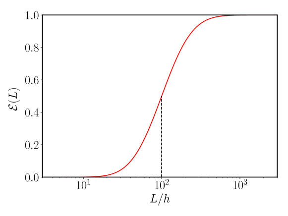
Figure 1: Breaking probability of a fragment as a function of the largest dimension $L$. The vertical dashed line indicates the threshold, here chosen as $L_{c}=100h$

A second length scale, $L_{c}$, also entered the present model, originating in the mechanical sugar lump approach, described heuristically by means of a breaking efficiency ${\cal E}(L)$ sigmoidal in $L$. For the sake of convenience, this efficiency was built here from the classical Gauss error function. It was therefore close to 1 above a threshold value $L_{c}$ (chosen large enough compared to $h$) and close to 0 below $L_{c}$. A representative example is shown in Fig. 1, with $L_{c}/h=100$. Note that throughout this paper, all lengths involved in the numerical model are scaled by the thickness $h$.

Qualitatively speaking, this feature of the model means that when the larger dimension $L$ is below the threshold value $L_{c}$, fragments will “almost never” break, even if they have not reached yet the limiting (approximately) cubic shape of fragments of size $\approx h$. For the sake of simplicity, the threshold value was assumed not to depend on plastic type or on residence time in the ocean, considering that weathering occurred from the moment the waste was thrown in the environment and quickly rendered all common plastics brittle. A unique $L_{c}$ was thus used for all fragments.

Technical details about the model are given in supplementary information A.

III Results and comparison with field data

In this whole section, we discuss the results obtained with the sugar lump model and systematically compare with what we called the standard model  [8, 11, 10], that is to say the case where fragments always break into two (identical) pieces at each generation, whatever their size.

Whenever possible and meaningful, we also compare our results with available field data. Therefore, one needs to assign a numerical correspondence between the physical time scale and the duration of a step in the iterative models. The fragmentation rate of plastic pieces can be assessed using accelerated aging experiments [24, 25, 26]. The half-life time, corresponding to the time when the average particle size is divided by 2, has been found around 1000 hours, which roughly corresponds to one year of solar exposition [26]. Hence, the iterative step $t$ used in all following sections can be considered to be in the order of one year. For typical plastic film dimensions, it is reasonable to assume that the thickness $h$ is between 10 and 50 $\mu$m, and the initial largest lateral dimension $L_{\mathrm{init}}$ is in the range of 1 to 5 cm. These characteristic lengths, together with the other length scales involved in this paper are positioned relative to each other in Fig. 2.

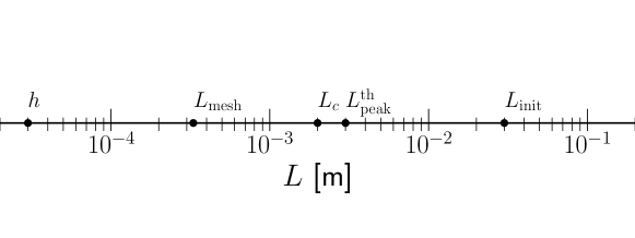
Figure 2: Characteristic length scales: film thickness $h$, mesh size $L_{\mathrm{mesh}}$, breaking threshold $L_{c}$, predicted peak position in the size distribution of fragments $L_{\mathrm{peak}}^{\mathrm{th}}$, and largest lateral initial dimension of fragments $L_{\mathrm{init}}$. Values $h=30~{}\mu$m and $L_{\mathrm{init}}=3$ cm have been chosen for being typical values. A mesh size $L_{\mathrm{mesh}}=330$ $\mu$m is representative of neuston or manta nets used for collecting plastics debris. The peak position $L_{\mathrm{peak}}^{\mathrm{th}}$ actually depends on time, and may become smaller than the threshold length $L_{c}$ as fragmentation proceeds.

III.1 Evolution of the size distribution and of the total abundance of fragments with time

The size distribution of plastic fragments over time is represented in Fig. 3 for the sugar lump and confronted to the standard model size distribution. The origin of time corresponds to the date when the very first plastic waste was dumped into the ocean.

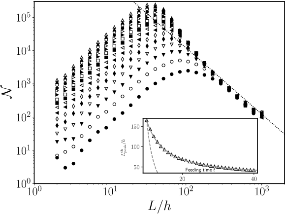
Figure 3: Evolution of the size distribution of fragments over time for a chosen threshold value $L_{c}/h=100$. For clarity, the number of fragments $\cal N$ as a function of fragment size $L/h$ is shown from $t=10$ ($\bullet$) to $t=40$ ($\triangle$), every two time steps. The dotted line represents–in the standard model–the expected size distribution. Inset: Variation of the peak position $L_{\mathrm{peak}}^{\mathrm{th}}$ with time, the continuous line being merely a guide to the eyes. The dashed line is the exponentially-decaying evolution of the smallest size reached at a given time $t$ in the standard model.

According to the standard model (see Eq. (7), Section A.1), the amount of particles as a function of their size follows a power law of exponent $-2$ which leads to a divergence of the number of particles at very small size (dotted line in Fig  3). For large MP, the prediction of the sugar lump model was broadly similar, i.e. following the same power law. By contrast, the existence of a mechanism inhibiting the break of smaller objects, as introduced in the sugar lump model, did lead to the progressive built of an abundance peak for intermediate size fragments due to the accumulation of fragments with size around $L_{c}$ (see Section A.3 for details). Moreover, the particle abundance at the peak increased with time while the peak position shifted towards smaller size classes. This shift was fast for the first generations, and then slowed down when time passes: The inset in Fig. 3 showed how the existence of a breaking threshold significantly slowed down the production of very small particles compared to the standard model. As can be observed from the inset in Fig. 3, the peak position $L_{\mathrm{peak}}^{\mathrm{th}}$, around $L_{c}$, decreased in a small range typically between 1.5$L_{c}$ and 0.5$L_{c}$ for time periods up to a few tens of years.

Let us now discuss the comparison to the experimental data. A sample of various field data from different authors  [8, 11, 10, 17, 27, 4] is displayed in Fig. 4. In order to obtain a collapse of the data points for large MPs, a vertical scaling factor has been applied, since abundance values from different sources can not be directly compared in absolute units. The two main features of these curves are: A maximum abundance at a value of a few millimeters (indicated by a gray arrow), and the collapse of the data points onto a single $1/L^{2}$ master curve (indicated by a dashed line). Note that data from Ref. [4] (black triangles) which is, to the best of our knowledge, the only data allowing a direct comparison of the amount of MP over the whole range of sizes from $10$ to $10^{4}~{}\mu$m, also demonstrates these features: After a small abundance peak followed by a decrease, one observes another increase when going to smaller sizes, as described in the introduction. This high population of small MP is most probably the result of delamination processes, which are not addressed here.

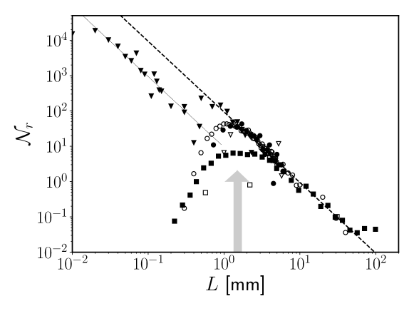
Figure 4: Re-scaled size distribution of fragments ${\cal N}_{r}$ as a function of their largest dimension $L$ from various field data: $\blacktriangledown$–Poulain, Mercier et al. [4]; $\square$–Eriksen, Lebreton et al. [10]; $\blacksquare$–Cozár, Etchevarría et al. [8]; $\triangledown$–ter Halle, Ladirat et al. [11]; $\bullet$–Tokai, Uchida et al. [17]; $\circ$–Isobe, Uchida et al. [27]. The two straight lines, dotted and dashed, are guides for the eye describing a $1/L^{2}$ scaling law.

The threshold value $L_{c}$ is presumably defined by the energy balance between the bending energy required for breaking a film and the available turbulent energy of the ocean. The bending energy depends on the film geometry and on the mechanical properties of the weathered polymer. As shown for a fiber by Brouzet et al [28, 22], the threshold $L_{c}$ is proportional to the fiber diameter $d$ and varies as

$$L_{c}=k\frac{E^{1/4}}{(\rho\eta\epsilon)^{1/8}}d$$ (1)

where $E$ is the Young modulus of the brittle polymer fiber, $\rho$ and $\eta$ are the mass density and viscosity of water, $\epsilon$ is the mean turbulent dissipation rate and $k$ is a prefactor in the order of 1. In two dimensions, the expression for the threshold $L_{c}$ is more complex, since it depends both on the width $\ell$ and thickness $h$ of the film. However, based on 2D mechanics, one can show that the order of magnitude and $h$-dependency for $L_{c}$ remain the same as in 1D, while the prefactor slightly varies with $\ell$. Reasonable assumptions on film geometry, mechanical properties of weathered brittle plastic and highly turbulent ocean events, such as made by Brouzet et al. [22] allowed us to evaluate that $L_{c}/h\approx 100$. For films of typical thicknesses lying between 10 and 50 $\mu$m, this gave a position of the peak between 1 and 5 mm in good agreement with the field data represented in Fig. 4. It would be delicate to refine more since plastic waste in the environment exhibits a large range of mechanical properties due to their various chemical nature (including oxidation state), macromolecular architecture, the presence of inorganic fillers, etc.

It is also interesting to discuss the power law exponent value exhibited by both standard and sugar-lump models at large MP sizes. In time-invariant models, the theoretical exponent actually varies with the dimensionality of the considered objects (fibers, films, lumps) ranging from $-1$ (fibers) to $-3$ (lumps). As expected, when the objects dimensionality is fixed, the value $-2$ observed in Fig. 3 for the sugar-lump model is due to the hypothesis of film-like pieces breaking along their larger dimension only, keeping their thickness constant. In the same way, regarding the laboratory experiments performed on glass fibers [22], the large MP distribution is compatible in the long-time limit with the expected $-1$ power law . Coming back to the field data as displayed in Fig. 4, one can note that for large MP all data points collapsed onto a single $1/L^{2}$ master curve. This suggests that either most collected waste comprises film-like objects breaking along their larger dimension only, or, perhaps more likely, that one collects a mixture of all three types of objects leading to an “average” exponent, obviously lying somewhere between $-1$ and $-3$, that turns out to be close to $-2$.

The total abundance ${\cal N}_{\mathrm{tot}}$ of fragments (all sizes included) as a function of time was represented in Fig. 5 for both the sugar lump and standard models. In the latter case, the abundance was simply described by an exponential law: ${\cal N}_{\mathrm{tot}}=[2^{t+1}-1]{\cal N}_{0}$ when the ocean was fed by a constant number ${\cal N}_{0}$ of (nearly identical) large fragments per iteration (Eq. 4, Section A.1). The sugar lump model predicted a time evolution which deviates from the standard model prediction: The increase of total abundance slowed down with time, due to the hindering of smaller fragments production, and the effect was all the more pronounced for larger threshold parameters $L_{c}$, as could have been expected. In the realistic case where $L_{c}/h\approx 100$, the increasing rate of fragments production became very small for the largest feeding times, as can be observed in Fig. 5 which showed that the number of MP would be multiplied every ten years by only a factor 2, compared to a factor of 1000 in the standard model. These theoretical results might explain why no clear temporal trend is observed in the field data [2].

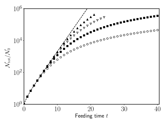
Figure 5: Total amount of fragments in the ocean (reduced units) as a function of time $t$ (i.e. number of iterative steps. One step approximately corresponds to one year), for different values of the size threshold $L_{c}$: $L_{c}=100h$–$\circ$; $L_{c}=30h$–$\blacksquare$; $L_{c}=10h$–$\triangledown$; $L_{c}=3h$–$\blacktriangle$. Dashed line: standard model. A value ${\cal N}_{0}=30$ has been chosen here

III.2 Role of the mesh size on the size distribution and on its temporal evolution

If one wants to go further in confronting models to field data, one needs to take into account that the experimental collection of particles in the environment always involves an observation window, and in particular a lower size limit $L_{\mathrm{mesh}}$, e.g. due to the mesh size of the net used during ocean campaigns. The very existence of a lower limit leads to the appearance of transitory and steady-state regimes for the temporal evolution of the number of collected particles, as will be shown below.

In the standard model case, when the feeding and breaking process started, larger size classes were first filled, while smaller size classes were still empty (Fig. 11, Section A.1). As long as the smaller fragments produced by the breaking process were larger than the lower size limit $L_{\mathrm{mesh}}$ of the collection tool, the number of collected fragments increased with time, de facto producing a transitory regime in the observed total abundance. The size of the smaller fragments reached $L_{\mathrm{mesh}}$ after a given number of fragmentation steps corresponding to the duration of the transitory regime:

$$t_{c}\approx 2\ln(L_{\mathrm{init}}/L_{\mathrm{mesh}})/\ln 2$$ (2)

where $L_{\mathrm{init}}$ is the initial largest dimension of the plastic fragments released into the ocean. From this time onward, both the size distribution and total number of collected fragments in the observation window no longer changed. Even though the production of fragments smaller than $L_{\mathrm{mesh}}$ continued to occur, as well as the continuous feeding of large-scale objects, one therefore observed a steady-state regime. This was illustrated in Fig. 6 for two different values of the mesh size $L_{\mathrm{mesh}}$ (full symbols $\bullet$ and $\blacksquare$).

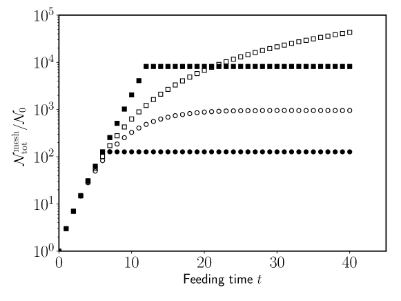
Figure 6: Time dependence of the total number of collected fragments ${\cal N}_{\mathrm{mesh}}$ (reduced units) for two different values of the mesh size in the case of the standard model (full symbols) and of the sugar lump model (empty symbols) with threshold $L_{c}/h=100$. Mesh size values for different symbol keys are, for the standard model, $L_{\mathrm{mesh}}/h$: $\bullet$, 93; $\blacksquare$, 6 and for the sugar lump model $L_{\mathrm{mesh}}/h$: $\circ$, 92; $\square$, 7

For the sugar lump model case, one needed to also consider the size threshold length scale $L_{c}$, below which fragmentation is inhibited. When $L_{c}$ was much smaller than $L_{\mathrm{mesh}}$, the threshold length $L_{c}$ was not in the observation window, hence the analysis was the same as in the standard case. At contrast, when $L_{c}$ was close to $L_{\mathrm{mesh}}$ or larger, the transitory regime was expected to exhibit two successive time dependencies. This behavior was displayed in Fig. 6 (empty symbols $\circ$ and $\square$) for the same mesh size values as in the standard model for comparison. At short times, since the smaller fragment size had not reached yet the breaking threshold $L_{c}$, the number of collected fragments followed the same law as in the standard case. When the smaller fragments got close to the size $L_{c}$, however, the inhibition of their breaking created an accumulation of fragments around $L_{c}$, hence the abundance peak. As a consequence, the increase in the total number of fragments slowed down. Since the abundance peak position shifted towards smaller values with time (Fig. 3, inset) albeit slowly, a final stationary state should be observed when the abundance peak position became significantly smaller than $L_{\mathrm{mesh}}$. As shown in Fig. 6, this occurred within the explored time window for large $L_{\mathrm{mesh}}$ ($\circ$), but the stationary state was not observed for small $L_{\mathrm{mesh}}$ ($\square$), presumably because our simulation had not explored times large enough. When the steady-state regime was reached, the number of fragments above $L_{\mathrm{mesh}}$, i.e. likely to be collected, remained constant with a value larger than that of the standard model, due to the overshoot induced by the accumulation on the right-hand side of the peak.

Let us recall that the characteristic fragmentation time, defined as the typical duration for a piece to break into two, has been evaluated at one year. In the case of the standard model, this meant that the size of each fragment was reduced by a factor 30 in about 10 years. Therefore, starting with debris size of the order of a centimeter, small MPs of typical size the mesh size (330 $\mu$m in Fig. 2) would be obtained within 10 years only. Thus, 10 years correspond to the duration of the transitory regime $t_{c}$ established in Eq. (2) and the oceans should be by far in the steady-state regime since the pollution started in the 1950’s. It is however no longer controversial nowadays that the standard (steady-state) model fails to describe the size distribution of the field data. On the contrary, the sugar lump model predicted the existence of an abundance peak, in agreement with what was observed during collection campaigns. This peak is due to the accumulation of fragments whose size is in the order of the breaking threshold $L_{c}$. As discussed in subsection III.1, the failure threshold $L_{c}$ could be soundly estimated to lie between $1$ and $5$ mm. Comparison with field data then corresponded to the case where $L_{c}$ was about ten times larger than the mesh size $L_{\mathrm{mesh}}$. As just shown in Fig. 6, this implied a drastic increase of duration of the transitory regime, that could be estimated to be above 100 years. These considerations lead us to the important conclusion that one is still nowadays in the transitory regime. Moreover, the sugar lump model also implies that the total abundance is correctly estimated through field data collection, i.e. that it is not biased by the mesh size. Because the peak position slowly shifted towards smaller sizes, the mesh size would eventually play a role, but at some much later point in time. Finally, let us recall that this paper did not take into account delamination processes, so the previous statement is only true for millimetric debris, that is to say debris produced through fragmentation, and that micrometric size debris might exhibit a completely different behavior, being in addition much more numerous.

III.3 Constant versus exponential feeding

In the results discussed in Section III.1, it was assumed that the rate of waste feeding in the ocean is constant with time. However, it is common knowledge that the production of plastics has increased significantly since the 1950’s. Geyer et al [30] show that the discarded waste follows the same trend. Data from the above-quoted article has been extracted and fitted in Fig. 7 and Fig. 8 with exponential laws ${\cal N}={\cal N}_{0}(1+\tau)^{t}$, where $\tau$ represents an annual growth rate, of plastic production and discarded waste respectively. For plastic production, the annual growth rate is found about 16$\%$ until 1974, the year of the oil crisis, and close to 6$\%$ after 1974 with, perhaps, an even further decrease of the rate in the recent years. Not unexpectedly, the same trends are found when considering the discarded waste, with growth rates, respectively, 17% and 5%. In order to discuss now the effects of an increasing waste feeding in the ocean, we injected for simplicity a single exponential with an intermediate rate of 7$\%$ in the two models.

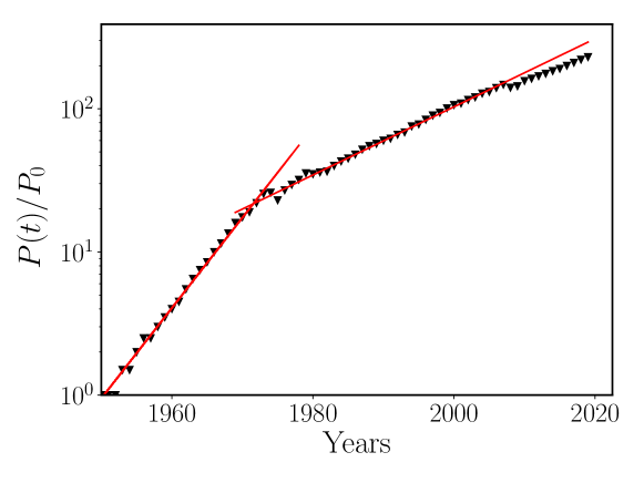
Figure 7: Global plastics production per year from 1950 onward, relative to $P_{0}=2\times 10^{6}$ t produced in 1950. A significant break in plastics production is observed in 1974. Solid lines: annual growth rates, about 16% or 6% per year before or after 1974, respectively

Figure 8: Estimated discarded plastic wastes, in relative units. A significant break in discarded waste is observed in 1974. Solid lines: annual growth rates, about 17% or 5% per year before or after 1974, respectively

When comparing this feeding law and the standard fragmentation law $[2^{t+1}-1]{\cal N}_{0}$, one easily concluded that the total number of plastics items in the ocean was mainly determined by the fragmentation rate, regardless of the feeding rate. In order to verify what happens in the case of the sugar lump model, where the fragmentation process was hindered, the size distributions for both feeding hypotheses were numerically compared in Figs. 9a and 9b, respectively after 14 and 40 years.

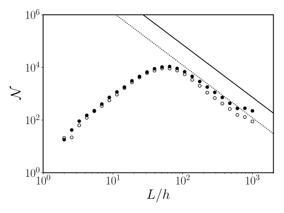
(a)

(b)

Figure 9: Comparison of the size distributions of fragments $\cal N$ for the two feeding modes : $\bullet$ exponential feeding, $\circ$ constant feeding, for (a) a small number of fragmentation steps and (b) a large number of fragmentation steps. Continuous and dotted straight lines are guides for the eyes for the –$L^{-2}$ scaling law

It could be observed that at short times, the size distribution was very little altered by the change in feeding. At longer times, a significant increase of the amount of the largest particles could be observed, while the amount of small particles was increasing much less. Besides, the size position of the abundance peak was almost not shifted.

The total amount of fragments was represented in Fig. 10 for the standard and sugar lump models for the two feeding cases considered. For exponential feeding, the sugar lump model still predicted a significant decrease in the rate of fragment generation over time, whereas one could have thought that exponential feeding could cancel out this slowdown.

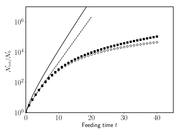
Figure 10: Total amount of fragments in the ocean (reduced units) as a function of time $t$ (arbitrary units), for standard (lines) and sugar lump (symbols) models and two feeding hypothesis, namely constant or exponential feedings. The inflation rate is 0 (empty symbols $\circ$ or dashed line) or $7$% (full symbols $\blacksquare$ or solid line). For the sugar lump model, the size threshold is $L_{c}=100h$

The conclusions drawn above, Section III.2 therefore remained valid in the more realistic case of an exponential feeding.

Finally, one should keep in mind that, if the feeding rate is a reasonable indicator of plastic pollution, since it describes the evolution over time of the total mass of plastics present in the ocean, it is not enough to properly describe plastic pollution. For a given mass, the number–hence size–of particles produced is the major factor in assessing potential impacts. Indeed, the smaller the size the larger the particles number concentration, the larger their specific area hence their adsorption ability and the larger the ensuing eco-toxicity. It was shown here that the mass of waste roughly doubles every 10 years, whereas the number of particles doubles every year, making fragmentation the main factor driving plastic pollution and impacts. A lot of studies are devoted to making a mass balance and understanding the fluxes of plastic waste  [30, 13, 31, 32] but, even in the case of a drastic immediate reduction of waste production, plastic pollution and impacts will affect the ocean life for still many years to come, due to fragmentation.

IV Conclusion

The generalist model presented here was based on a few sound physical assumptions and shed new light on global temporal trends in the distribution of microplastics at the surface of the oceans. The model showed that the existence of a physical size threshold below which fragmentation is strongly inhibited, lead to the accumulation of fragments at a given size, in line with what is observed in the field data. In other words, if one does collect much fewer particles in the range $150$ $\mu$m–$1$ mm  [4], it is because only a few of them is actually generated by fragmentation at this scale. One would not necessarily need to invoke any other mechanism or bias such as ingestion by living organisms [33] or the mesh size of collection nets [14, 16], to explain the field data for floating debris. As a consequence, the observed distribution does reflect, in our opinion, the real distribution of MPs at the surface of the ocean, down to 100 $\mu$m. Besides, the sugar lump model implied a slowdown in the rate of MPs production by fragmentation, due to the fact that fragmentation is inhibited when particles approach the threshold size. This may explain the absence of a clear increase in the MP numbers in different geographical areas [2].

Two other general facts have been pointed out in this paper:

• For large MP, the predicted size distribution followed a power law, whose exponent depends on the dimensionality of the object (-1 for a fiber, -2 for a film and -3 for a lump). It is therefore worth sorting out collected objects according to their geometry, as it is done for instance when fibers are separated from 2D objects [16]. It is however interesting to note that, when the objects are not sorted in this way, an “average value” -2 is found for the exponent.

• The model took into account an exponentially-increasing waste feeding rate. We have fitted the plastic production since the 1950’s and found that there is not one but two exponential laws, the second one, slower than the first one, being visible after the oil crisis in 1974. Comparing this feeding to the exponential fragmentation ratio, we showed that the number of fragments was mainly predicted by the fragmentation process, regardless of the feeding details.

To go further and estimate absolute values of MP concentrations in the whole range of sizes, it would be necessary, on one hand, to take into account delamination in order to get small particles distribution. On the other hand, one should also be aware of the spatial heterogeneity of particles concentration and therefore an interesting development could be to combine fragmentation with flow models developed for instance in Refs. [32, 34].

CRediT author statement

Matthieu George:  Conceptualization, Validation, Writing – Review & Editing, Project administration
Frédéric Nallet:  Methodology, Software, Writing – Review & Editing
Pascale Fabre:  Conceptualization, Validation, Writing – Review & Editing, Funding acquisition

Declaration of interests

The authors declare that they have no known competing financial interests or personal relationships that could have appeared to influence the work reported in this paper

Appendix A Supporting information

A.1 Standard model

In this model, as pictorially represented in Fig. 11, the ocean is fed at each iteration $n$ with a fixed number $a_{0}$ of large 2D-like objects, mimicking plastic films.

Figure 11: Schematics of iterative size classes filling by the standard model. Horizontal axis, rightwards: size (or generation) index $p$; Vertical axis, downwards: time index $n$. Short horizontal arrows stand for the feeding process. Wavy arrows stand for the fragmentation process. The shade of gray represents the weathering of a given object, that is to say the time spent in the ocean

Neglecting size and shape dispersity for convenience, all 0^th-generation objects are assumed to be large square platelets of lateral size $L_{\mathrm{init}}$ and thickness $h$, with $L_{\mathrm{init}}\gg h$. Between consecutive iteration steps, fragmentation produces $p^{th}$-generation objects, by splitting in two equal parts $(p-1)^{th}$-generation objects, thus generating square platelets when $p$ is even, but rectangular platelets with aspect ratio 2:1 for odd $p$. If size is measured by the diagonal, a $p^{th}$-generation object has size $\sqrt{2}L_{\mathrm{init}}/2^{p/2}$ (even $p$) or $\sqrt{5}L_{\mathrm{init}}/2^{(p+1)/2}$ (odd $p$). With size classes described by the number of $p^{th}$-generation objects at iteration step $n$, $C(n,p)$, the filling law of size classes is:

$$\begin{array}[]{rcll}C(n,0)&=&a_{0}&\\ C(n,p)&=&0&\mathrm{~{}if~{}}p>n\\ C(n,p)&=&2C(n-1,p-1)&\mathrm{~{}if~{}}1\leq p\leq n\end{array}$$ (3)

The set of equations (3) is readily solved: $C(n,p)=2^{p}a_{0}$ for $0\leq p\leq n$, and $C(n,p)=0$ for $p>n$. Since size $L$ scales with generation index $p$ as $2^{-p/2}$, the steady-sate scaling for the filling of size classes is $C\propto L^{-2}$.

The cumulative abundance $S_{n}\equiv\sum_{p}C(n,p)$ at iteration step $n$ is also easily obtained:

$$S_{n}=\left[2^{n+1}-1\right]a_{0}$$ (4)

and displayed as a dashed line in Figs. 5 and 10.

As noticed in Ref. [11] where experimental data and model predictions are matched together, the standard model fails for small objects, and this occurs when a (nearly) cubic shape is reached. Since the typical (lateral) size of $p^{th}$-generation objects is $\approx L_{\mathrm{init}}/2^{p/2}$, the limit is reached for

$$p_{\mathrm{max}}\approx 2\frac{\log\frac{L_{\mathrm{init}}}{h}}{\log 2}$$ (5)

that is to say in about 20 generations with the rough estimate $L_{\mathrm{init}}/h=10^{3}$. The set of equations describing the size-class filling law has to be altered to take into account this limit. Assuming for simplicity that $p_{\mathrm{max}}$-generation objects cannot be fragmented anymore (“atomic” fragments), this set of equations becomes:

$$\begin{array}[]{rcll}C(n,0)&=&a_{0}&\\ C(n,p)&=&0&\mathrm{~{}if~{}}p>n\mathrm{~{}or~{}}p>p_{\mathrm{max}}\\ C(n,p)&=&2C(n-1,p-1)&\mathrm{~{}if~{}}1\leq p<p_{\mathrm{max}}\mathrm{~{}and~{}}p\leq n\\ C(n,p_{\mathrm{max}})&=&C(n-1,p_{\mathrm{max}})+2C(n-1,p_{\mathrm{max}}-1)&\mathrm{~{}if~{}}n>p_{\mathrm{max}}\end{array}$$ (6)

As shown by the explicit solution, Eq. (7) below, the last line in this set of equations leads to an accumulation of “atomic” fragments (see also Fig. 12 for a pictorial representation of this feature)

$$\begin{array}[]{rcll}C(n,p)&=&2^{p}a_{0}&\mathrm{~{}if~{}}0\leq p\leq n<p_{\mathrm{max}}\\ C(n,p_{\mathrm{max}})&=&\left(n+1-p_{\mathrm{max}}\right)2^{p_{\mathrm{max}}}a_{0}&\mathrm{~{}if~{}}n\geq p_{\mathrm{max}}\\ C(n,p)&=&0&\mathrm{~{}for~{}other~{}cases}\end{array}$$ (7)

associated to a significant (exponential to linear) slowing down of the cumulative abundance:

$$S_{n}=\left[2^{p_{\mathrm{max}}}\left(2+n-p_{\mathrm{max}}\right)-1\right]a_{0}$$ (8)

for iteration steps $n\geq p_{\mathrm{max}}$.

Figure 12: Time-invariant features of the standard model, as long as the “atomic limit” has not been reached yet. Symbol keys and time indices: $\bullet$, $n=10$; $\circ$, $n=20$; $\blacktriangledown$, $n=40$; $\triangledown$, $n=80$. “Atomic” limit reached for generation index $p_{\mathrm{max}}$ chosen equal to $18$

A.2 Standard model with inflation

As a first extension of the standard model, inflation in the feeding of the ocean with large 2D-like objects is now considered. Taking simultaneously into account the “atomic” nature of small fragments beyond $p_{\mathrm{max}}$ generations, the size-class filling set of equations (3) has to be replaced by:

$$\begin{array}[]{rcll}C(n,0)&=&a_{0}\left(1+\tau\right)^{n}&\\ C(n,p)&=&0&\mathrm{~{}if~{}}p>n\mathrm{~{}or~{}}p>p_{\mathrm{max}}\\ C(n,p)&=&2C(n-1,p-1)&\mathrm{~{}if~{}}1\leq p<p_{\mathrm{max}}\mathrm{~{}and~{}}p\leq n\\ C(n,p_{\mathrm{max}})&=&C(n-1,p_{\mathrm{max}})+2C(n-1,p_{\mathrm{max}}-1)&\mathrm{~{}if~{}}n>p_{\mathrm{max}}\end{array}$$ (9)

Size classes are now described by $C(n,p)=2^{p}\left(1+\tau\right)^{n-p}a_{0}$ for $0\leq p\leq n$ as long as the generation index $p$ remains smaller than $p_{\mathrm{max}}$ and $C(n,p_{\mathrm{max}})=2^{p_{\mathrm{max}}}\left[\left(1+\tau\right)^{n-p_{\mathrm{max}}+1}-1\right]a_{0}/\tau$ for $n\geq p_{\mathrm{max}}$. Whereas the filling of the size class associated to “atomic” fragments was linear in $n$ without inflation, it becomes here exponential. Consequently, the cumulative abundance, definitely slowed down, remains exponential in $n$ for $n>p_{\mathrm{max}}$:

$$S_{n}=\left\{\left(1+\tau\right)^{n}\left[\frac{\left(\frac{2}{1+\tau}\right)^{p_{\mathrm{max}}}-1}{1-\tau}\right]+2^{p_{\mathrm{max}}}\frac{\left(1+\tau\right)^{n-p_{\mathrm{max}}+1}-1}{\tau}\right\}a_{0}$$ (10)

As long as the “atomic limit” is not reached, the cumulative abundance exhibits a simpler form, namely:

$$S_{n}=\left[2^{n+1}-\left(1+\tau\right)^{n+1}\right]\frac{a_{0}}{1-\tau}$$ (11)

that does not significantly differ from Eq. (4). The time-invariant features of the size distribution are nevertheless modified in two respects (see Fig. 13):

Figure 13: Time-invariant features of the standard model, taking into account inflation at a 7% yearly rate. Symbol keys and time indices: $\bullet$, $n=10$; $\circ$, $n=20$; $\blacktriangledown$, $n=40$; $\triangledown$, $n=80$. Superimposed dashed lines: fits to scaling law ${\cal N}\propto 1/L^{\nu}$ with $\nu\approx 1.8$

1. Inflation spoils the strict time-invariant feature previously observed for the size distribution ${\cal N}(L)$;

2. A (nearly) time-invariant behavior remains as far as scaling is concerned, since ${\cal N}\propto 1/L^{\nu}$, but $\nu$ does depend, albeit rather weakly, on the time index $n$, while being significantly smaller than $2$. Fitting data to a power law, an exponent $\nu$ close to $1.8$ is obtained for inflation $\tau=7\%$.

A.3 Sugar lump model

Taking inspiration from the standard model, Section A.1, at each iteration the ocean is fed with large parallelepipedic fragments of length $L$, width $\ell$ and thickness $h$, where $h$ is much smaller than the other two dimensions and length $L$ is, by convention, larger than width $\ell$. Some size dispersity is introduced when populating the largest size class, by randomly distributing $L$ in the interval $[0.9L_{\mathrm{init}},L_{\mathrm{init}}]$, and $\ell$ in $[0.7L_{\mathrm{init}},0.9L_{\mathrm{init}}]$, but $h$ is kept fixed. The number of objects feeding the system can be controlled at each iteration step, and two simple limits have been investigated: Constant, or exponentially-growing feeding rates, mimicking two variants of the Standard model, Sections A.1 and A.2, respectively. Size-classes evenly sampling (in logarithmic scale) the full range of $L/h$, $[1,L_{\mathrm{init}}/h]$ are populated by sorting into the proper size class the fragments present in the system. Except for the $0^{\mathrm{th}}$, initialization step, these fragments are either $0^{\mathrm{th}}$-generation fragments just introduced into the system, obviously belonging to the largest size class, or $g$-generation fragments ($g\geq 1$) that have been “weathered” during the time step from step $n$ to step $n+1$ and then split, with a $L$-dependent efficiency, into two smaller fragments. As explained in Section II, the splitting process, albeit random, explicitly ensures the existence of an “atomic” limit: Fragments belonging to the smallest size class cannot be fragmented any further. As tentatively illustrated in Fig. 14, a special feature of the model is that generations ($g$) and size-class ($p$) indices have to be distinguished because, at contrast with the standard model, although for a given fragment a “weathering” event ($n\rightarrow n+1$) is always associated to an “aging” event ($g$ increased by one), it is not always associated to populating one or two lower-size classes (and simultaneously decreasing by 1 the abundance of the considered size-class) because the splitting process is not $100$% efficient.

Figure 14: Schematics of iterative size classes filling for the sugar lump model. Horizontal axis, rightwards: size index $p$; Vertical axis, downwards: time index $n$. Short horizontal arrows stand for the feeding process. Full or dotted wavy arrows stand for a 100%, or partially efficient fragmentation process. The shade of gray represents the weathering (time spent in the ocean) of a given object. Note that the size threshold for fragmentation (vertical thick line between size classes 3 and 4) leads to a decoupling between size and age

Keeping track of abundances in terms of time ($n$), age ($g$) and size ($p$) being computationally demanding for exponentially-growing populations, our simulations have been limited to, at most, $n=g=40$. The number of distinct size classes has also been limited to 28, as this corresponds to the number of size-classes reported in Ref. [8].

References

- Ritchie and Roser [2018] H. Ritchie and M. Roser, Plastic pollution, Our World in Data (2018), https://ourworldindata.org/plastic-pollution.
- Galgani et al. [2021] F. Galgani, A. S.-o. Brien, J. Weis, C. Ioakeimidis, Q. Schuyler, I. Makarenko, H. Griffiths, J. Bondareff, D. Vethaak, A. Deidun, P. Sobral, K. Topouzelis, P. Vlahos, F. Lana, M. Hassellov, O. Gerigny, B. Arsonina, A. Ambulkar, M. Azzaro, and M. J. Bebianno, Are litter, plastic and microplastic quantities increasing in the ocean?, Microplastics and Nanoplastics 1, 2 (2021).
- Eriksen et al. [2023] M. Eriksen, W. Cowger, L. M. Erdle, S. Coffin, P. Villarrubia-Gómez, C. J. Moore, E. J. Carpenter, R. H. Day, M. Thiel, and C. Wilcox, A growing plastic smog, now estimated to be over 170 trillion plastic particles afloat in the world’s oceans—urgent solutions required, PLOS ONE 18, 1 (2023).
- Poulain et al. [2019] M. Poulain, M. J. Mercier, L. Brach, M. Martignac, C. Routaboul, E. Perez, M. C. Desjean, and A. ter Halle, Small microplastics as a main contributor to plastic mass balance in the North Atlantic Subtropical Gyre, Environmental Science & Technology 53, 1157 (2019), https://doi.org/10.1021/acs.est.8b05458 .
- Pabortsava and Lampitt [2020] K. Pabortsava and R. S. Lampitt, High concentrations of plastic hidden beneath the surface of the Atlantic Ocean, Nature Communications 11, 10.1038/s41467-020-17932-9 (2020).
- Weiss et al. [2021] L. Weiss, W. Ludwig, S. Heussner, M. Canals, J.-F. Ghiglione, C. Estournel, M. Constant, and P. Kerhervé, The missing ocean plastic sink: Gone with the rivers, Science 373, 107 (2021), https://www.science.org/doi/pdf/10.1126/science.abe0290 .
- George and Fabre [2021] M. George and P. Fabre, Floating plastics in oceans: A matter of size, Current Opinion in Green and Sustainable Chemistry 32, 100543 (2021).
- Cózar et al. [2014] A. Cózar, F. Echevarría, J. I. González-Gordillo, X. Irigoien, B. Úbeda, S. Hernández-León, Á. T. Palma, S. Navarro, J. García-de Lomas, and A. Ruiz, Plastic debris in the open Ocean, Proceedings of the National Academy of Sciences 111, 10239 (2014).
- Isobe et al. [2014] A. Isobe, K. Kubo, Y. Tamura, S. Kako, E. Nakashima, and N. Fujii, Selective transport of microplastics and mesoplastics by drifting in coastal waters, Marine Pollution Bulletin 89, 324 (2014).
- Eriksen et al. [2014] M. Eriksen, L. C. M. Lebreton, H. S. Carson, M. Thiel, C. J. Moore, J. C. Borerro, F. Galgani, P. G. Ryan, and J. Reisser, Plastic pollution in the world’s oceans: More than 5 trillion plastic pieces weighing over 250,000 tons afloat at sea, PLOS ONE 9, 1 (2014).
- ter Halle et al. [2016] A. ter Halle, L. Ladirat, X. Gendre, D. Goudouneche, C. Pusineri, C. Routaboul, C. Tenailleau, B. Duployer, and E. Perez, Understanding the fragmentation pattern of marine plastic debris, Environmental science & technology 50, 5668 (2016).
- Lebreton et al. [2018] L. Lebreton, B. Slat, F. Ferrari, B. Sainte-Rose, J. Aitken, R. Marthouse, S. Hajbane, S. Cunsolo, A. Schwarz, A. Levivier, K. Noble, P. Debeljak, H. Maral, R. Schoeneich-Argent, R. Brambini, and J. Reisser, Evidence that the Great Pacific Garbage Patch is rapidly accumulating plastic, Scientific Reports 8, 4666 (2018).
- Lebreton et al. [2019] L. Lebreton, M. Egger, and B. Slat, A global mass budget for positively buoyant macroplastic debris in the ocean, Scientific Reports 9, 12922 (2019).
- Isobe et al. [2019] A. Isobe, S. Iwasaki, K. Uchida, and T. Tokai, Abundance of non-conservative microplastics in the upper ocean from 1957 to 2066, Nature Communications 10, 417 (2019).
- Kataoka et al. [2019] T. Kataoka, Y. Nihei, K. Kudou, and H. Hinata, Assessment of the sources and inflow processes of microplastics in the river environments of Japan, Environmental Pollution 244, 958 (2019).
- Lindeque et al. [2020] P. K. Lindeque, M. Cole, R. L. Coppock, C. N. Lewis, R. Z. Miller, A. J. Watts, A. Wilson-McNeal, S. L. Wright, and T. S. Galloway, Are we underestimating microplastic abundance in the marine environment? A comparison of microplastic capture with nets of different mesh-size, Environmental Pollution 265, 114721 (2020).
- Tokai et al. [2021] T. Tokai, K. Uchida, M. Kuroda, and A. Isobe, Mesh selectivity of neuston nets for microplastics, Marine Pollution Bulletin 165, 112111 (2021).
- Andrady [2017] A. L. Andrady, The plastic in microplastics: A review, Marine Pollution Bulletin 119, 12 (2017).
- Cózar et al. [2015] A. Cózar, M. Sanz-Martín, E. Martí, J. I. González-Gordillo, B. Ubeda, J. Á. Gálvez, X. Irigoien, and C. M. Duarte, Plastic accumulation in the mediterranean sea, PLOS ONE 10, 1 (2015).
- Enders et al. [2015] K. Enders, R. Lenz, C. A. Stedmon, and T. G. Nielsen, Abundance, size and polymer composition of marine microplastics m in the Atlantic Ocean and their modelled vertical distribution, Marine pollution bulletin 100, 70 (2015).
- Van Sebille et al. [2015] E. Van Sebille, C. Wilcox, L. Lebreton, N. Maximenko, B. D. Hardesty, J. A. Van Franeker, M. Eriksen, D. Siegel, F. Galgani, and K. L. Law, A global inventory of small floating plastic debris, Environmental Research Letters 10, 124006 (2015).
- Brouzet et al. [2021] C. Brouzet, R. Guiné, M.-J. Dalbe, B. Favier, N. Vandenberghe, E. Villermaux, and G. Verhille, Laboratory model for plastic fragmentation in the turbulent ocean, Phys. Rev. Fluids 6, 024601 (2021).
- Aoki and Furue [2021] K. Aoki and R. Furue, A model for the size distribution of marine microplastics: A statistical mechanics approach, PLOS ONE 16, 1 (2021).
- Julienne et al. [2019] F. Julienne, F. Lagarde, and N. Delorme, Influence of the crystalline structure on the fragmentation of weathered polyolefines, Polymer Degradation and Stability 170, 109012 (2019).
- Julienne et al. [2022] F. Julienne, F. Lagarde, J.-F. Bardeau, and N. Delorme, Thin polyethylene (LDPE) films with controlled crystalline morphology for studying plastic weathering and microplastic generation, Polymer Degradation and Stability 195, 109791 (2022).
- Menzel et al. [2022] T. Menzel, N. Meides, A. Mauel, U. Mansfeld, W. Kretschmer, M. Kuhn, E. M. Herzig, V. Altstädt, P. Strohriegl, J. Senker, and H. Ruckdäschel, Degradation of low-density polyethylene to nanoplastic particles by accelerated weathering, Science of the Total Environment 826, 154035 (2022).
- Isobe et al. [2015] A. Isobe, K. Uchida, T. Tokai, and S. Iwasaki, East asian seas: A hot spot of pelagic microplastics, Marine Pollution Bulletin 101, 618 (2015).
- Brouzet et al. [2014] C. Brouzet, G. Verhille, and P. Le Gal, Flexible fiber in a turbulent flow: A macroscopic polymer, Phys. Rev. Lett. 112, 074501 (2014).
- [29] Provided that, of course, the depletion of very large objects that originates from the absence of feeding is disregarded.
- Geyer et al. [2017] R. Geyer, J. R. Jambeck, and K. L. Law, Production, use, and fate of all plastics ever made, Science Advances 3, e1700782 (2017), https://www.science.org/doi/pdf/10.1126/sciadv.1700782 .
- Cordier and Uehara [2019] M. Cordier and T. Uehara, How much innovation is needed to protect the ocean from plastic contamination?, Science of The Total Environment 670, 789 (2019).
- Sonke et al. [2022] J. E. Sonke, A. M. Koenig, N. Yakovenko, O. Hagelskjær, H. Margenat, S. V. Hansson, F. De Vleeschouwer, O. Magand, G. Le Roux, and J. L. Thomas, A mass budget and box model of global plastics cycling, degradation and dispersal in the land-ocean-atmosphere system, Microplastics and Nanoplastics 2, 28 (2022).
- Dawson et al. [2018] A. L. Dawson, S. Kawaguchi, C. K. King, K. A. Townsend, R. King, W. M. Huston, and S. M. Bengtson Nash, Turning microplastics into nanoplastics through digestive fragmentation by Antarctic krill, Nature Communications 9, 1001 (2018).
- van Sebille et al. [2020] E. van Sebille, S. Aliani, K. L. Law, N. Maximenko, J. M. Alsina, A. Bagaev, M. Bergmann, B. Chapron, I. Chubarenko, A. Cózar, P. Delandmeter, M. Egger, B. Fox-Kemper, S. P. Garaba, L. Goddijn-Murphy, B. D. Hardesty, M. J. Hoffman, A. Isobe, C. E. Jongedijk, M. L. A. Kaandorp, L. Khatmullina, A. A. Koelmans, T. Kukulka, C. Laufkötter, L. Lebreton, D. Lobelle, C. Maes, V. Martinez-Vicente, M. A. M. Maqueda, M. Poulain-Zarcos, E. Rodríguez, P. G. Ryan, A. L. Shanks, W. J. Shim, G. Suaria, M. Thiel, T. S. van den Bremer, and D. Wichmann, The physical oceanography of the transport of floating marine debris, Environmental Research Letters 15, 023003 (2020).