Reducing False Alarms in Video Surveillance by Deep Feature Statistical Modeling

Abstract

Detecting relevant changes is a fundamental problem of video surveillance. Because of the high variability of data and the difficulty of properly annotating changes, unsupervised methods dominate the field. Arguably one of the most critical issues to make them practical is to reduce their false alarm rate. In this work, we develop a method-agnostic weakly supervised a-contrario validation process, based on high dimensional statistical modeling of deep features, to reduce the number of false alarms of any change detection algorithm. We also raise the insufficiency of the conventionally used pixel-wise evaluation, as it fails to precisely capture the performance needs of most real applications. For this reason, we complement pixel-wise metrics with object-wise metrics and evaluate the impact of our approach at both pixel and object levels, on six methods and several sequences from different datasets. Experimental results reveal that the proposed a-contrario validation is able to largely reduce the number of false alarms at both pixel and object levels.

1 Introduction

Video change detection is a fundamental problem in computer vision and the first step of many applications. While it is an easy task for humans in many contexts, it turns out to be very difficult to automate due to the wide range of possible scenarios.

In the domains of security and surveillance, change detection can be used for spotting temporal anomalies such as suspicious individuals or stolen objects [23, 28]. In urban scenarios, it can be exploited to analyze common activities such as monitoring illegal parking of vehicles [29]. Change detection may also serve climate and humanitarian causes. Satellite image time series can be used to monitor urban development [20] of specific regions and the variability of gas concentrations in the atmosphere across time [32, 33].

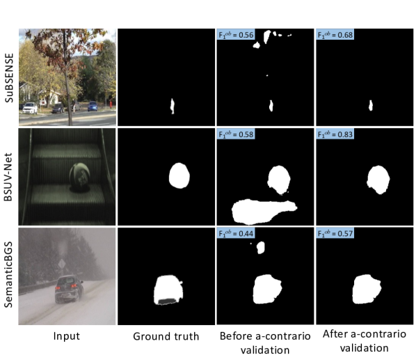
Figure 1: Sample results of the proposed a-contrario validation process for three different background subtraction algorithms. As shown, the proposed a-contrario validation is able to remove false positives of large and small sizes, while keeping true detections. The object-wise F-1 score of the corresponding sequence is highlighted in each case.

Traditional change detection methods work by learning a statistical model of a scene under normal conditions. This so-called background model is based on past samples [4, 41]. When a new frame is provided, it is compared to the background reference model, which can lead to a detection and/or to an update of this background model. Traditional pixel-wise methods are convenient because only a short local training is required, and the computational complexity remains low. Nevertheless, these techniques are limited by the locality of the features, such as RGB pixels, which makes them prone to false alarms. To overcome this problem, deep learning has been used to leverage the ability of deep neural networks (DNNs) to learn suitable, high-level descriptors of a scene. Despite having shown improvements over traditional video change detection methods [7, 2, 37], such approaches are constrained by their supervised nature and experience a substantial decrease of performance when tested on out of distribution data. Recently, some works have focused on exploiting the semantic information provided by DNNs in an unsupervised manner [6, 31]. These methods are more robust than classical approaches and do not require labeled examples. However, they are still sensitive to false positives in complex environments such as dynamic backgrounds or adverse weather conditions.

Decreasing the number of false positives in unsupervised methods is a high priority goal. Indeed, a significant number of false alarms may saturate a detection system or require human intervention, which is expensive and time consuming. Change detection methods are conventionally evaluated on pixel-wise metrics, regardless of the spatial organization of faulty pixels: multiple small false detections are counted on par with a single false detection with equivalent area. As a result, pixel-wise scores may not realistically represent the performance of target applications. The number of false alarms is better evaluated at the object level than at the pixel level, because the cost of a false alarm is generally independent of its size. Hence, we shall favor object-wise performance metrics, where by object we understand a connected component.

In this work, we present a weakly supervised a-contrario validation process, based on high-dimensional modeling of deep features, to largely reduce the number of false positives at both the pixel and object levels. The contributions of our work are as follows:

• We propose a method agnostic, weakly supervised a-contrario validation process that can significantly reduce false alarms in video change detection. To the best of our knowledge, this is the first work to use the a-contrario framework at the DNN feature level for a detection problem.

• We evaluate our work on six methods at both pixel and object levels. Furthermore, we test them on a set of sequences from different datasets, namely CDNet [19, 45], LASIESTA [10] and J. Zhong and S. Sclaroff [47].

• Our results show a considerable increase in object-wise performance metrics, while also improving or maintaining the pixel-wise results. Figure 1 illustrates this improvement.

2 Related works

The detection of temporal anomalies in a video sequence or an image time series is known as change detection. It is difficult to find a definition of temporal anomalies that suits all cases. The methods in the literature look for changes with respect to previously observed examples that are semantically meaningful for the desired downstream task. Change detection algorithms in the literature can be categorized into traditional and neural network-based methods.

Traditional change detection Traditional change detection methods use statistical computer vision techniques to model the background of a scene and update it online [40]. These approaches commonly follow a three-step workflow consisting in 1) building a background model of the scene, 2) comparing the new observed frames to the background model, and 3) updating the model accordingly. Background modeling consists in building a faithful probabilistic representation of the past, which is used as a reference for further observed examples. The seminal example of this approach is the adaptive Gaussian Mixture Model (GMM), first introduced by Stauffer and Grimson [42], which modeled each pixel with a mixture of $K$ Gaussian functions. Several modifications of their method have been proposed [48, 21, 30] to improve performance and efficiency. Later methods proposed to model the background using a buffer of past samples, which can alleviate computational complexity. New samples are compared against the stored examples based on a consensus. The popular unsupervised methods ViBE [4] and SuBSENSE [41] use such consensus-based algorithms. During inference, a new unseen frame is compared to the generated background model using an error metric that maps pixels to either background or foreground clusters, producing a binary mask with this two-level information.

Deep learning-based change detection methods More recent works have exploited current deep learning algorithms to replace one or more steps of the traditional flow. Braham and Van Droogenbroeck [7] show that the complex background modeling task can be simplified by training a CNN with scene-specific examples. An autoencoder-based architecture called FgSegNet is proposed in [25], which adapts a VGG-16 [39] architecture into a triplet framework, processing images at three different scales. Tezcan et al. [43] proposed BSUV-Net, which trains a scene agnostic network so that it can be tested on new, unseen scenes without individually fine-tuning the network. A newer version of their approach, BSUV-Net 2.0 [44], was later proposed. The ability of DNNs to learn suitable, high-level descriptors of a scene has proved to yield better results than traditional approaches [7, 2, 37]. Nevertheless, supervised methods require large amounts of annotated data, a tedious and time consuming task. Furthermore, the performance of supervised methods often declines on out of domain examples. Consequently, unsupervised methods are often chosen over recent supervised methods [15, 5]. For this reason, several recent works have focused on leveraging DNN high-level representations without supervision. Braham et al. [6] proposed SemanticBGS, where a classic method is complemented with semantic information provided by a pre-trained network. Moreover, a real-time version of the same approach named RT-SemanticBGS [9] was later introduced. G-LBM, introduced by Rezaei et al. [34], models the background of a scene with a generative adversarial network (GAN) in the presence of noise and sparse outliers.

Unsupervised DNN-based methods achieve a better performance than traditional approaches. Nonetheless, they still fall behind supervised methods in popular benchmarks. Similarly to classic methods, these techniques may detect a substantial number of false alarms, which can critically saturate detection systems.

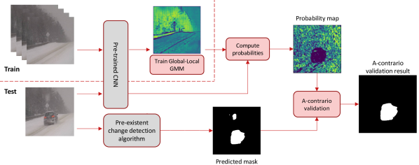
Figure 2: The proposed deep feature a-contrario validation extracts the representations given by a pre-trained network and models them with a global-to-local mixture of Gaussians. For a new, unseen frame, it computes the probability map of observing a temporal anomaly using the trained GMM. Given a change mask predicted by any algorithm in the literature, a validation process based on a-contrario theory addresses all detected regions and removes false alarms.

Statistical modeling for video scene understanding Surveillance applications need to distinguish foreground from background elements so that target instances can be further processed. Early methods attempted to statistically model appearance information with parametric models such as GMMs [42, 48, 21, 30]. However, background modeling in complex scenarios (e.g. dynamic backgrounds or adverse weather conditions) has proved to be challenging for those approaches. Other works introduce optical flow to understand the motion patterns of a scene. For example, Saleemi et al. [38] proposed to model the motion patterns with a mixture of Gaussians using optical flow. Similarly, Ghahremannezhad et al. [16] proposed a method for real-time foreground segmentation modeling optical flow with a GMM. Some recent works have propsoed to model the feature space of deep neural networks for image anomaly detection. PaDiM, proposed by Defard et al. [11], is a framework that models patches of a DNN feature map with a Gaussian model for anomaly detection and localization. Artola et al. [1] generalized this attempt with GLAD, a method that learns a robust GMM globally, and then localizes the learned Gaussians with a spatial weight map. Modeling spatial features in a high-dimensional space has shown promising results at recognizing complex patterns.

A-contrario detection theory The a-contrario detection theory is a mathematical formulation of the non-accidentalness principle, which states that an observed structure is meaningful only when the relation between its parts is too regular to be the result of an accidental arrangement of independent parts [46, 27]. The a-contrario methodology [14, 12] allows one to control the number of false alarms by considering an observed structure only when the expectation of its occurrences is small in a stochastic background model. The Number of False Alarms (NFA) of an event $e$ observed up to a precision $z(e)$ in the background model $\mathcal{H}_{0}$ is defined by

$$\mathrm{NFA}(e)=N_{T}\cdot\text{I\kern-1.49994ptP}[Z_{\mathcal{H}_{0}}(e)\geq z(e)],$$ (1)

where $\text{I\kern-1.49994ptP}[Z_{\mathcal{H}_{0}}(e)\geq z(e)]$ is the probability of obtaining a precision $Z_{\mathcal{H}_{0}}(e)$ better or equal to the observed one $z(e)$ in the background model $\mathcal{H}_{0}$. The term $N_{T}$ corresponds to the number of tests, following the statistical multiple hypothesis testing framework [18]. A small NFA indicates that the event $e$ is unlikely to be randomly observed in the background model $\mathcal{H}_{0}$. Hence, the lower the NFA the more meaningful the event. A value $\epsilon$ is specified and candidates with $\mathrm{NFA}<\epsilon$ are accepted as valid detections. It can be shown [14] that in these conditions $\epsilon$ is an upper-bound to the expected number of false detections under $\mathcal{H}_{0}$.

A-contrario methods have been previously proposed to address computer vision problems. Lisani and Ramis developed a method in [26] that applied an a-contrario methodology on a normal distribution for the detection of faces in images. In surveillance, a-contrario methods have been used mainly in the remote sensing field, [20, 35], where the temporal difference between images is large, and no tracking of temporal objects is feasible. Grompone et al. [20] proposed an a-contrario method based on a uniform distribution and a greedy algorithm to compute candidate regions, detecting visible ground areas in satellite imagery.

3 Pixel and object-wise evaluation

Change detection algorithms tend to be evaluated on pixel-wise metrics. Whilst this approach allows one to assess how well methods classify pixels into foreground or background clusters, it often fails to represent the performance needs of real applications. Detection systems today tend to consider detections as sets of connected components instead of independent pixels. Then, they process each detection separately for further analysis. An algorithm with high pixel-wise evaluation scores might still predict a considerable amount of false alarms at the object level, which can lead to bottlenecks in the system. Focusing on the performance at the object level will provide a more accurate account of the usability of methods for surveillance applications. Hence, reducing false positives at the object level is one of the most important elements to minimize in order to increase speed and avoid system saturation.

Consequently, we consider both pixel-wise and object-wise evaluation metrics to analyze the performance of our work and existing algorithms. We emphasize our evaluation on the reduction of false alarms and the accuracy of the detections. Let tn, tp, fn, fp be the usual pixel-wise number of true negatives, true positives, false negatives and false positives, respectively. Our experiments consider the following pixel-wise metrics:

• Precision: $\textsc{pr}^{pi}=\textsc{tp}/(\textsc{tp}+\textsc{fp})$

• Recall: $\textsc{re}^{pi}=\textsc{tp}/(\textsc{tp}+\textsc{fn})$

• False Positive Rate: $\textsc{fpr}^{pi}=\textsc{fp}/(\textsc{fp}+\textsc{tn})$

• Percentage of Wrong Classifications:
  $\textsc{pwc}^{pi}=100\times(\textsc{fn}+\textsc{fp})/(\textsc{tp}+\textsc{fn}+\textsc{fp}+\textsc{tn})$

• F-measure: $\textsc{f${}_{1}$}^{pi}=2(\textsc{pr}^{pi}\times\textsc{re}^{pi})/(\textsc{pr}^{pi}+\textsc{re}^{pi})$.

We also evaluate the results at the object level, where $\textsc{tp}^{ob}$, $\textsc{fn}^{ob}$ and $\textsc{fp}^{ob}$ now correspond to true positives, false negatives and false positives for sets of connected components. To define those, we take the approach of Chan et al. [8] and use a variation of the traditional intersection over union (IoU) first introduced by Rottman et al. [36]. Unlike the conventional IoU, which penalizes cases where a ground truth region is fragmented into multiple predictions by assigning each prediction a moderate IoU score, the adapted metric, named sIoU, does not penalize predictions of a segment when the remaining ground truth is sufficiently covered by other predicted segments.

More formally, let $\mathcal{K}$ be the set of anomalous components in the ground truth, and $\hat{\mathcal{K}}$ the set of anomalous components predicted by a change detection algorithm. hen, the sIoU metric consists in a mapping $sIoU:\mathcal{K}\rightarrow[0,1]$ defined for $k\in\mathcal{K}$ by

$$\begin{split}sIoU(k):=\frac{|k\cap\hat{\mathcal{K}}(k)|}{|(k\cup\hat{\mathcal{K}}(k))\backslash\mathcal{A}(k)|}\\ \text{with}\quad\hat{\mathcal{K}}(k)=\bigcup_{\hat{k}\in\hat{\mathcal{K}},\hat{k}\cap k\neq\varnothing}\hat{k},\end{split}$$ (2)

where $\mathcal{A}(k)=\{z\in k^{\prime}:k^{\prime}\in\mathcal{K}\backslash\{k\}\}$. The introduction of $\mathcal{A}(k)$ excludes all pixels from the union if and only if they correctly intersect with another ground-truth component. Hence, given a threshold $\tau\in[0,1)$, we define a target $k\in\mathcal{K}$ as $\textsc{tp}^{ob}$ if $sIoU>\tau$, and as $\textsc{fn}^{ob}$ otherwise. Then, $\textsc{fp}^{ob}$ is computed as the positive predictive value (PPV) for $\hat{k}\in\hat{\mathcal{K}}$, defined as:

$$PPV(\hat{k}):=\frac{|\hat{k}\cap\mathcal{K}(\hat{k})|}{|\hat{k}|}.$$ (3)

Thus, $\hat{k}\in\hat{\mathcal{K}}$ is $\textsc{fp}^{ob}$ if $PPV(\hat{k})\leq\tau$. Lastly, the sIoU-based F-measure is computed as follows:

• F-measure: $\textsc{f${}_{1}$}^{sIoU}(\tau)=\frac{\textsc{tp}^{ob}(\tau)}{\textsc{tp}^{ob}(\tau)+\textsc{fn}^{ob}(\tau)+\textsc{fp}^{ob}(\tau)}$

We follow the approach of Chan et al. and average the results for different thresholds $\tau=\{0.25,0.5,0.75\}$.

4 Our approach

We propose to supplement any change detection method from the literature with a final a-contrario validation step applied on connected components. Such validation is based on a statistical model of the DNN representations of the scene and requires no annotation. Given a set of input frames of a sequence, we obtain its feature representations at stages 1 and 2 of a pre-trained ResNet-50 [22] architecture. We use a backbone pre-trained on ImageNet [13] with self-supervision using the VicReg method [3]. Figure 2 shows a high-level diagram of the proposed approach, and the next subsections describe its different parts in detail.

4.1 Background feature modeling

We model the extracted deep representations with a mixture of Gaussians to assess the likelihood of an image patch to be a part of the background. For that we extend the GLAD [1] framework to the background modeling of videos. This requires no dense annotations but just a selection of training frames with none or few anomalies present, thus we coin our approach as weakly supervised. A mixture is first learned globally, i.e. without taking into consideration the spatial location of the data points. This yields a first Gaussian mixture model $\theta=(\phi_{i},\mu_{i},\Sigma_{i})_{i\in\{1,\dots,K\}}$, where $\mu_{i}$ and $\Sigma_{i}$ are the mean and variance components, while $\phi_{i}$ are the mixture weights. Then, a local model is derived by assigning position-dependent weights for each Gaussian, so that an image position is represented by a local mixture of the most relevant Gaussian distributions. This gives a localized model that depends on the pixel position $(x,y)$ such that $\theta(x,y)=(\phi_{i}(x,y),\mu_{i},\Sigma_{i})_{i\in\{1,\dots,K\}}$, where $\mu_{i}$ and $\Sigma_{i}$ do not depend on the position $(x,y)$. This global to local approach enables one to exploit information from other similar pixels, to build a good representation of each observed pixel. The probability of observing p at position $(x,y)$ is

$$\mathbb{P}\big{(}\textbf{p}~{}|~{}\theta(x,y)\big{)}=\sum_{i=1}^{K}\phi_{i}(x,y)\mathbb{P}(\textbf{p}~{}|~{}\mu_{i},\Sigma_{i}),$$ (4)

where only the weights $\phi_{i}(x,y)$ depend on the position. Then, the $p\mbox{-}\mathrm{value}$ of a given pixel p at position $(x,y)$ is

$$p\mbox{-}\mathrm{value}\big{(}\textbf{p}~{}|~{}\theta(x,y)\big{)}=\int\limits_{\hskip 34.1433pt\mathcal{D}(\textbf{p}|\theta(x,y))}\mathbb{P}\big{(}\textbf{q}~{}|~{}\theta(x,y)\big{)}\,d\textbf{q},$$ (5)

where $\mathcal{D}(\textbf{p}|\theta(x,y))=\big{\{}\textbf{q}~{}|~{}\mathbb{P}(\textbf{q}|\theta(x,y))\leq\mathbb{P}(\textbf{p}|\theta(x,y))\big{\}}$. This quantity cannot be easily computed, but an upper-bound can be derived. We can invert the sum of the GMM and the integral of the $p$-value to get $K$ Gaussian integrals. However the set $\mathcal{D}$ cannot be computed, so we introduce $\mathcal{D}_{i}(\textbf{p}|\theta(x,y))=\big{\{}\textbf{q}~{}|~{}\phi_{i}(x,y)\mathbb{P}(\textbf{q}~{}|~{}\mu_{i},\Sigma_{i})\leq\mathbb{P}(\textbf{p}|\theta(x,y))\big{\}}$ which contains it ($\mathcal{D}\subseteq\mathcal{D}_{i}$). So we find ourselves with the upper bound

$$p\mbox{-}\mathrm{value}\big{(}\textbf{p}~{}|~{}\theta(x,y)\big{)}\leq\sum_{i=1}^{K}\int\limits_{\hskip 36.98857pt\mathcal{D}_{i}(\textbf{p}|\theta(x,y))}\mathbb{P}(\textbf{q}~{}|~{}\mu_{i},\Sigma_{i})\,d\textbf{q}.$$ (6)

These integrals are equivalent to the $\chi^{2}$ survival function; in the case where the features are of even dimension they are equal to a finite sum that can be computed exactly (see the supplementary material).

4.2 A-contrario validation

We propose an a-contrario method designed to control the number of false alarms on any change detection method. A change candidate will only be meaningful when the expectation of all its independent parts is low. In our case, we define the background model $\mathcal{H}_{0}$ as the local Gaussian mixture $\theta$ learned during training. Thus, we define the number of false alarms $\mathrm{NFA}(R)$ over a region $R$, as:

$$\mathrm{NFA}(R)=N_{T}\cdot\text{I\kern-1.49994ptP}[Z_{\theta}(R)\geq z(R)],$$ (7)

where $z(R)$ measures how anomalous the observed values in region $R$ are. The corresponding random variable $Z_{\theta}$ is a random vector with the same dimension as the number of pixels of $R$. Then, assuming pixel independence (see below), we propose to measure anomaly relative to a Gaussian mixture $\theta$ by defining the probability term of (7) as:

$$\text{I\kern-1.49994ptP}[Z_{\theta}(R)\geq z(R)]=\prod_{\textbf{p}\in R}p\mbox{-}\mathrm{value}\big{(}\textbf{p}~{}|~{}\theta(x,y)\big{)},$$ (8)

where $p\mbox{-}\mathrm{value}\big{(}\textbf{p}~{}|~{}\theta(x,y)\big{)}$, given by Equation (5), is evaluated on each pixel p of the region $R$.

We need to define the number of tests $N_{T}$ to complete the NFA formulation (7). $N_{T}$ is related to the total number of candidate regions that can, in theory, be considered for evaluation. Inspired by the approach in [20], we will consider regions of any shape formed by 4-connected pixels. Regions of pixels with 4-connectivity are known as polyominoes [17, 18]. The exact number $b_{n}$ of different polyomino configurations of a given size $n$ is not known in general; however, a good estimate [24] is given by $b_{n}\approx\alpha\frac{\beta^{n}}{n}$ where $\alpha\approx 0.317$ and $\beta\approx 4.06$. Additionally, we need to consider that any pixel in the image can be the center of a region and that a region can be of size from 1 to $XY$, where $X$ and $Y$ are the width and height of the image, respectively. Thus, we can define the number of tests $N_{T}$ as

$$N_{T}=X^{2}Y^{2}\alpha\frac{\beta^{n}}{n},$$ (9)

where $n=|R|$ is the size of the region $R$. Notice that this is not exact, as Equation (9) allows for some potential polyominoes extending outside of the image boundaries, but it is an approximation of the same magnitude.

Deep feature representations are computed via spatial convolutions. Hence, assuming pixel independence over an entire region is inaccurate. To compensate for this, we introduce a correcting exponent $\frac{1}{c_{f}}$ where $c_{f}$ corresponds to the area of the receptive field of a given stage, i.e. $c_{f}=35$ for stage 1 and $c_{f}=91$ for stage 2. We then compute a geometric mean of the probability term on the receptive field. All in all, Equation (7) can be expressed as

$$\mathrm{NFA}(R)=X^{2}Y^{2}\alpha\frac{\beta^{n}}{n}\left(\prod_{\textbf{p}\in R}p\mbox{-}\mathrm{value}\big{(}\textbf{p}~{}|~{}\theta(x,y)\big{)}\right)^{\frac{1}{c_{f}}}$$ (10)

A region $R$ with $\mathrm{NFA}(R)<\epsilon$ is declared a change detection. Since the $\mathrm{NFA}$ can take very extreme values, $\log(\mathrm{NFA})$ is often easier to handle.

5 Experiments

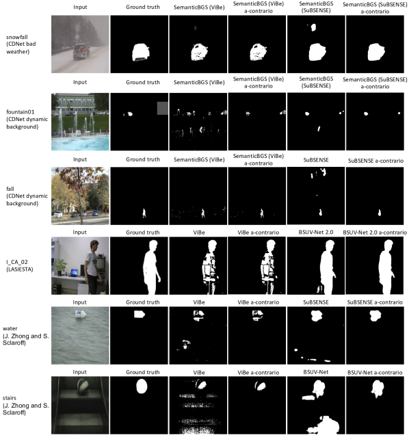
Figure 3: Detection results before and after the a-contrario validation, on sequences taken in different datasets. For each sequence, results are shown for two of the evaluated change detection algorithms.

Implementation details We trained a GMM on each sequence setting $K=1000$ initial Gaussian distributions and we let GLAD remove unnecessary Gaussians, as addressed by its authors as the best option. For training, we selected the first few hundred subsequent frames of each scene without any obvious anomalies. For the sequences where anomalies are continuously present (e.g. cars driving by a road), a temporal median filter is applied to filter them out. For the scenes where first frames contain only a few outliers, we kept them in the training set. The a-contrario validation was applied with a threshold $\epsilon=1$, and we computed the geometric mean of the NFA scores of each stage. For simplicity, the sequences and their ground truths were resized to 256$\times$256.

Results on the CDNet benchmark CDNet [19, 45] is a benchmark for video change detection consisting of 53 videos divided into 11 categories. Each category corresponds to a specific challenge such as shadow or lowFramerate. It provides pixel-wise annotations for all frames except the first few hundred, which can be used for initialization and we use to train our models. We compute the proposed approach on all categories of the dataset except for categories cameraJitter and PTZ, since we assume the camera is static. We evaluated the impact of our approach on a range of methods for the pixel and object-wise metrics introduced in Section 3. The selected methods were ViBe [4], SuBSENSE [41], SemanticBGS [6], BSUV-Net [43], BSUVFPM-Net [43] and BSUV-Net 2.0 [44]. The classic ViBe and SuBSENSE are still popular and remain on the state of the art. SemanticBGS is the best performing unsupervised method in CDNet, and the BSUV family of methods are supervised, scene agnostic approaches. Table 1 shows the relative change percentage when applying the proposed a-contrario validation compared to the methods alone on all the CDNet dataset (except cameraJitter and PTZ). Furthermore, we selected two categories that are substantially prone to false alarms: dynamic background and bad weather, and show their results separately on Table 2 and Table 3. For the tables containing the exact metric scores, refer to the supplementary material. Formally, we denote by $S_{b}$ and $S_{a}$ the metric scores before and after the a-contrario validation, respectively. We then compute the percentage improvement as

$$\text{ {relative change percentage} }=\frac{S_{a}-S_{b}}{S_{b}}\times 100.$$ (11)

As observed, our approach is able to largely improve the object-wise metrics in all methods, while maintaining or improving their pixel-wise counterparts. Notice that in some cases, such as for ViBe, the percentage improvement is surprisingly large. This occurs as a consequence of removing all FPs that correspond to isolated pixels, as the method commonly yields significant segmentation noise in complex scenes. Figure 3 shows examples of the achieved qualitative results for different sequences and methods. Lastly, the proposed method proved to be robust to anomalies in the training data, yielding weak clusters and low probabilities for such occurrences, as per the cases where a few anomalies were present in the training set.

Method	pixel-wise			object-wise
	$\textsc{fpr}^{pi}\downarrow$	$\textsc{pwc}^{pi}\downarrow$	$\textsc{f${}_{1}$}^{pi}\uparrow$	$\textsc{sIoU}\uparrow$	$\textsc{f${}_{1}$}^{sIoU}\uparrow$
ViBe [4]	-64.45 %	-22.81 %	13.40 %	204.00 %	36.12 %
SuBSENSE [41]	-20.36 %	-3.06 %	-1.20 %	14.96 %	8.69 %
SemanticBGS (with ViBe) [6]	-41.10 %	-6.70 %	3.93 %	119.07 %	95.50 %
SemanticBGS (with SuBSENSE) [6]	-19.05 %	-0.15 %	-1.73 %	31.13 %	19.78 %
BSUV-Net 2.0 [44]	-11.61 %	3.88 %	-1.74 %	24.86 %	9.45 %
BSUV-Net FPM [43]	0.02 %	2.02 %	-0.78 %	9.75 %	3.06 %
BSUV-Net [43]	-3.13 %	1.21 %	-1.19 %	16.60 %	7.13 %

Table 1: Results on the CDNet benchmark, which includes all categories with the exception of cameraJitter and PTZ, since we assume the camera is static. Both pixel-wise and obejct-wise metrics are provided.

Method	pixel-wise			object-wise
	$\textsc{fpr}^{pi}\downarrow$	$\textsc{pwc}^{pi}\downarrow$	$\textsc{f${}_{1}$}^{pi}\uparrow$	$\textsc{sIoU}\uparrow$	$\textsc{f${}_{1}$}^{sIoU}\uparrow$
ViBe [4]	-88.97 %	-93.07 %	158.96 %	5159.21 %	5350.29 %
SuBSENSE [41]	-27.25 %	-3.00 %	1.21 %	37.99 %	28.28 %
SemanticBGS (with ViBe) [6]	-82.42 %	-77.27 %	31.40 %	1583.91 %	1472.55 %
SemanticBGS (with SuBSENSE) [6]	-1.60 %	-0.03 %	0.01 %	30.09 %	21.92 %
BSUV-Net 2.0 [44]	-6.36 %	-0.55 %	-0.02 %	49.20 %	32.77 %
BSUV-Net FPM [43]	27.41 %	18.07 %	-0.63 %	8.46 %	2.76 %
BSUV-Net [43]	-3.29 %	0.11 %	-0.22 %	30.26 %	16.44 %

Table 2: Results on the dynamic background category of the CDNet benchmark. Both pixel-wise and obejct-wise metrics are provided.

Method	pixel-wise			object-wise
	$\textsc{fpr}^{pi}\downarrow$	$\textsc{pwc}^{pi}\downarrow$	$\textsc{f${}_{1}$}^{pi}\uparrow$	$\textsc{sIoU}\uparrow$	$\textsc{f${}_{1}$}^{sIoU}\uparrow$
ViBe [4]	-85.43 %	-13.38 %	21.98 %	301.73 %	331.69 %
SuBSENSE [41]	-11.02 %	-1.04 %	0.38 %	22.20 %	15.65 %
SemanticBGS (with ViBe) [6]	-50.35 %	-0.58 %	-0.48 %	234.33 %	227.09 %
SemanticBGS (with SuBSENSE) [6]	-9.68 %	-0.57 %	0.09 %	61.75 %	57.21 %
BSUV-Net 2.0 [44]	-1.36 %	0.51 %	-0.17 %	33.77 %	13.00 %
BSUV-Net FPM [43]	-0.72 %	0.14 %	-0.10 %	12.21 %	5.50 %
BSUV-Net [43]	-3.24 %	0.38 %	-0.17 %	28.06 %	12.79 %

Table 3: Results on the bad weather category of the CDNet benchmark. Both pixel-wise and obejct-wise metrics are provided.

Results on LASIESTA sequences The LASIESTA (Labeled and Annotated Sequences for Integral Evaluation of SegmenTation Algorithms) dataset [10] is a fully annotated benchmark for change detection and foreground segmentation proposed by Cuevas et al. It is composed of different indoor and outdoor scenes organized in categories, such as camouflage, shadows or dynamic background. Consequently, we evaluate all sequences with the exception of the ones with camera motion and simulated motion, as we assume the camera is stable. We train on the first 50 frames, without checking whether they contain desired detections. The impact of our approach is evaluated in Table 4. In this case, SemanticGBS is not considered because the required semantic segmentation pre-computed maps are only provided for CDNet sequences. We can observe that most methods alone already reach good pixel-wise scores and that the a-contrario validation does not decrease them. Furthermore, object-wise metrics improve in all cases. This demonstrates the efficacy of our approach in scenarios with both indoor and outdoor scenes.

Method	pixel-wise			object-wise
	$\textsc{fpr}^{pi}\downarrow$	$\textsc{pwc}^{pi}\downarrow$	$\textsc{f${}_{1}$}^{pi}\uparrow$	$\textsc{sIoU}\uparrow$	$\textsc{f${}_{1}$}^{sIoU}\uparrow$
ViBe [4]	-2.07 %	-0.82 %	0.26 %	58.67 %	44.75 %
SuBSENSE [41]	-0.02 %	0.02 %	-0.02 %	1.00 %	0.38 %
BSUV-Net 2.0 [44]	-0.14 %	0.00 %	-0.01 %	10.16 %	3.38 %
BSUV-Net FPM [43]	-0.14 %	-0.01 %	0.00 %	5.30 %	1.82 %
BSUV-Net [43]	-0.16 %	0.02 %	-0.01 %	7.65 %	2.79 %

Table 4: Results of the impact of our approach in a set of change detection methods on the selected sequences of LASIESTA dataset. Both pixel-wise and obejct-wise metrics are provided.

Results on sequences from J. Zhong and S. Sclaroff [47] Lastly, we evaluated our method on two sequences from J. Zhong and S. Sclaroff [47] containing challenging dynamic backgrounds. One of them shows an escalator moving continuously, while the other displays a floating plastic bottle. In each case, sequences with and without the target objects are provided; we used the latter for training and tested on the former. We evaluated our approach on the same methods as for LASIESTA sequences. The results, reported in Table 5, show a clear improvement of both pixel-wise and object-wise scores in all methods with the exception of BSUV 2.0, where the pixel-wise F-score drops slightly.

Method	pixel-wise			object-wise
	$\textsc{fpr}^{pi}\downarrow$	$\textsc{pwc}^{pi}\downarrow$	$\textsc{f${}_{1}$}^{pi}\uparrow$	$\textsc{sIoU}\uparrow$	$\textsc{f${}_{1}$}^{sIoU}\uparrow$
ViBe [4]	-96.44 %	-83.28 %	83.28 %	2312.40 %	3365.97 %
SuBSENSE [41]	-87.99 %	-70.06 %	30.50 %	379.91 %	205.67 %
BSUV-Net 2.0 [44]	-54.04 %	0.32 %	-4.85 %	70.46 %	15.02 %
BSUV-Net FPM [43]	-88.02 %	-80.95 %	39.17 %	99.97 %	40.90 %
BSUV-Net [43]	-80.93 %	-77.95 %	30.04 %	81.93 %	30.49 %

Table 5: Results of the impact of our approach in a set of change detection methods on the two sequences from J. Zhong and S. Sclaroff [47]. Both pixel-wise and obejct-wise metrics are provided.

Could the obtained drastic reduction of false alarms be achieved by a simpler method than the a-contrario test? An obvious argument that comes to mind is that eliminating small sized objects might lead to similar performance. It could indeed be argued that most datasets contain large true positives, compared to the size of predicted false positives. Therefore, we checked if simply removing all small detections could lead to significant improvement of the false alarm rate. To study the capability of our approach in discriminating FPs from TPs regardless of the size of the detections, we analyzed their separability in relation to the size and the proposed $\log(\mathrm{NFA})$ score. Doing so also leads to find an optimal value of the threshold $\epsilon$. Figure 4 compares the separability of FPs and TPs based on the region size against the $\log(\mathrm{NFA})$ score, for the results predicted by SuBSENSE for the sequence escalator. This particular example shows how FPs and TPs are not separable by region size, but the a-contrario assessment provides a clear separation instead. Additional examples are provided in the supplementary material, for other sequences and methods. The value of $\log(\epsilon)$ is then set to 0 (thus $\epsilon$=1), which provides a reasonable separation of FPs and TPs without discarding a high number of true detections. Moreover, the selection of $\epsilon$=1 holds a strong significance as it corresponds to an expected number of false alarms equal to one.

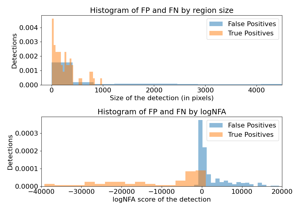
Figure 4: Comparison of the histograms of TP and FP computed by the SuBSENSE algorithm for the sequence escalator, by size of the detection (top) and by the $\log(\mathrm{NFA})$ score (bottom). As shown, filtering out small detections is not efficient. The $\log(\mathrm{NFA})$ provides a more suitable separation.

6 Conclusion

In this work, we introduced statistical modeling approach of deep features for the reduction of false alarms in video surveillance applications. In Section 5 a series of experiments were conducted to measure the impact of the proposed a-contrario validation on several change detection algorithms. The results indicate that substantial improvement is achieved in object-wise measures in virtually all cases, without decreasing the pixel-wise results. The ability to reduce the number of false alarms by such large margins without hampering detection accuracy is an important step towards real automation of surveillance systems. Moreover, we showed the capability of our approach to discard FPs regardless of their size. To the best of our knowledge, this is the first work that uses statistical modeling in the deep feature space for video surveillance applications.

Limitations and future work While our work successfully decreases the number of false alarms and improves several algorithms on short and mid size sequences, each sequence needs to be trained offline. This compromises the method in long, evolving sequences. Hence, future work will focus on the an online version to adapt to such cases.

Reducing false alarms in video surveillance by deep feature statistical modeling - Supplementary material

This supplementary section complements the description, analysis and claims of the main text. Firstly, Section A explains in detail the computation of the p-value, introduced in Section 4, for a mixture of Gaussians of features of even dimension. Secondly, the complete quantitative results obtained for all datasets, with and without the a-contrario validation, are provided in Section B. Lastly, complementary examples of the separability of TP and FP by region size versus by $logNFA$ score are provided in Section C.

Appendix A Computation of p-value for features of even dimension

We seek to calculate a p-value for a mixture of Gaussians. For simplicity, we will consider a mixture of classical Gaussian distributions without location information

$$\mathbb{P}\big{(}\textbf{p}~{}|~{}\theta\big{)}=\sum_{i=1}^{K}\phi_{i}\mathbb{P}(\textbf{p}~{}|~{}\mu_{i},\Sigma_{i}).$$ (12)

We then define the p-value as the integral of the density where the probability is lower than the probability density $\mathbb{P}(\textbf{p}|\theta)$:

$$\begin{array}[]{r c l}p\mbox{-}\mathrm{value}\big{(}\textbf{p}~{}|~{}\theta\big{)}&=&\int\limits_{\hskip 34.1433pt\mathcal{D}(\textbf{p}|\theta)}\mathbb{P}\big{(}\textbf{q}~{}|~{}\theta\big{)}\,d\textbf{q}\\ &=&\sum_{i=1}^{K}\phi_{i}\int\limits_{\hskip 17.07164pt\mathcal{D}(\textbf{p}|\theta)}\mathbb{P}(\textbf{q}~{}|~{}\mu_{i},\Sigma_{i})\,d\textbf{q},\end{array}$$ (13)

where $\mathcal{D}(\textbf{p}|\theta)=\big{\{}\textbf{q}~{}|~{}\mathbb{P}(\textbf{q}|\theta)\leq\mathbb{P}(\textbf{p}|\theta)\big{\}}$. This yields a weighted sum of Gaussian integrals. Nevertheless, the domain $\mathcal{D}$ is impossible to compute due to the interactions between the components. In this situation we introduce $\mathcal{D}_{i}(\textbf{p}|\theta)=\big{\{}\textbf{q}~{}|~{}\phi_{i}\mathbb{P}(\textbf{q}~{}|~{}\mu_{i},\Sigma_{i})\leq\mathbb{P}(\textbf{p}|\theta)\big{\}}$, which contains it ($\mathcal{D}\subseteq\mathcal{D}_{i}$) because if $\textbf{q}\in\mathcal{D}$ then $\forall i$ we have $\phi_{i}\mathbb{P}(\textbf{q}~{}|~{}\mu_{i},\Sigma_{i})\leq\mathbb{P}(\textbf{q}|\theta)\leq\mathbb{P}(\textbf{p}|\theta)$, hence $q\in\mathcal{D}_{i}$. We thus find an upper bound of the p-value by replacing $\mathcal{D}$ by the corresponding $\mathcal{D}_{i}$ in the integrals, i.e.

$$p\mbox{-}\mathrm{value}\big{(}\textbf{p}~{}|~{}\theta\big{)}\leq\sum_{i=1}^{K}\phi_{i}\int\limits_{\hskip 17.07164pt\mathcal{D}_{i}(\textbf{p}|\theta)}\mathbb{P}(\textbf{q}~{}|~{}\mu_{i},\Sigma_{i})\,d\textbf{q}.$$

To solve this, we first rewrite the condition for a feature to be included in $D_{i}$, showing that this is the outside area of an ellipsoid characterized by $R_{i}^{2}$ as defined below:

$${rclm}\phi_{i}\mathbb{P}(\textbf{q}~{}|~{}\mu_{i},\Sigma_{i}) \leq \mathbb{P}(\textbf{p}|\theta) \Leftrightarrow$$ (14)

$$\frac{\phi_{i}}{\sqrt{(2\pi)^{d}|\Sigma_{i}|}}\exp-\frac{1}{2}(q-\mu_{i})^{T}\Sigma_{i}^{-1}(q-\mu_{i}) \leq \mathbb{P}(\textbf{p}|\theta) \Leftrightarrow$$

$$(q-\mu_{i})^{T}\Sigma_{i}^{-1}(q-\mu_{i}) \geq R_{i}^{2}$$    where

$$\max(0,-2\log\mathbb{P}(\textbf{p}|\theta)+2\log\phi_{i}-\log|\Sigma_{i}|-d\log 2\pi) = R_{i}^{2}.$$

We then introduce two changes of variables to facilitate the integral. The first one is a normalization of the Gaussian, $u=\Sigma_{i}^{-1/2}(p-\mu_{i})$ with the determinant of the Jacobian $|J|=\sqrt{|\Sigma_{i}|}$, so that

$$\begin{array}[]{r c l}\int\limits_{\hskip 17.07164pt\mathcal{D}_{i}(\textbf{p}|\theta)}\mathbb{P}(\textbf{q}~{}|~{}\mu_{i},\Sigma_{i})\,d\textbf{q}&=&(2\pi)^{-d/2}\int\limits_{\hskip 17.07164ptu^{T}u\geq R_{i}^{2}}e^{-\frac{1}{2}u^{T}u}\,du.\end{array}$$ (15)

Subsequently, we shift to hyper spherical coordinates through another change of variable:

$$\begin{array}[]{r l}u_{1}&=r\cos{\theta_{1}}\\ u_{2}&=r\sin{\theta_{1}}\cos{\theta_{2}}\\ \vdots&=\vdots\\ u_{d-2}&=r\sin{\theta_{1}}\ldots\sin{\theta_{d-2}}\cos{\theta_{d-1}}\\ u_{d-1}&=r\sin{\theta_{1}}\ldots\sin{\theta_{d-2}}\sin{\theta_{d-1}}.\end{array}$$ (16)

The determinant of the Jacobian of this change is $|J|=r^{d-1}\prod_{k=1}^{d-2}\sin^{d-k-1}\theta_{k}$. Thus, we have the integral

$$\begin{array}[]{r c l}(2\pi)^{-d/2}\int\limits_{\hskip 17.07164ptu^{T}u\geq R_{i}^{2}}e^{-\frac{1}{2}u^{T}u}\,du&=&(2\pi)^{-d/2}\int_{0}^{2\pi}d\theta_{d}\prod_{k=1}^{d-2}\int_{0}^{\pi}\sin^{d-k-1}\theta_{k}d\theta_{k}\int_{R_{i}}^{+\infty}r^{d-1}\exp-\frac{1}{2}r^{2}\,dr.\end{array}$$ (17)

We first integrate the angles

$$\begin{array}[]{r c l}\prod_{k=1}^{d-2}\int_{0}^{\pi}\sin^{d-k-1}\theta_{k}d\theta_{k}&=&2\frac{\pi^{d/2}}{\Gamma(d/2)}.\end{array}$$ (18)

Then, we recognize the probability density of $\chi^{2}$ in the integral and therefore the whole is the survival function of $\chi^{2}$, such that

$$\begin{array}[]{r c l}\int\limits_{\hskip 17.07164pt\mathcal{D}_{i}(\textbf{p}|\theta)}\mathbb{P}(\textbf{q}~{}|~{}\mu_{i},\Sigma_{i})\,d\textbf{q}&=&\int_{R_{i}}^{+\infty}\frac{1}{2^{d/2-1}\Gamma(d/2)}r^{d-1}e^{-\frac{1}{2}r^{2}}\,dr\\ &=&\int_{R_{i}^{2}}^{+\infty}\frac{1}{2^{d/2}\Gamma(d/2)}x^{d/2-1}e^{-\frac{1}{2}x}\,dx\\ &=&\textbf{SF}_{\chi^{2}}(R_{i}^{2}).\end{array}$$ (19)

The $r$ integral can be computed via integration by parts, and the result depends on whether the dimension $d$ of the features is even or odd. We will first see the even case $d=2m$:

$$\begin{array}[]{r c l}\int_{R_{i}}^{+\infty}r^{2m-1}e^{-\frac{1}{2}r^{2}}\,dr&=&R_{i}^{2m-2}e^{-\frac{1}{2}R_{i}^{2}}+(2m-2)\int_{R_{i}}^{+\infty}r^{2m-3}e^{-\frac{1}{2}r^{2}}\,dr\\ &=&R_{i}^{2m-2}e^{-\frac{1}{2}R_{i}^{2}}+(2m-2)\left[R_{i}^{2m-4}e^{-\frac{1}{2}R_{i}^{2}}+(2m-4)\int_{R_{i}}^{+\infty}r^{2m-5}e^{-\frac{1}{2}r^{2}}\,dr\right]\\ &\vdots&\\ &=&\sum_{j=1}^{m-1}\frac{(m-1)!}{j!}2^{m-1-j}R_{i}^{2j}e^{-\frac{1}{2}R_{i}^{2}}+2^{m-1}(m-1)!\int_{R_{i}}^{+\infty}re^{-\frac{1}{2}r^{2}}\\ &=&\sum_{j=1}^{m-1}\frac{(m-1)!}{j!}2^{m-1-j}R_{i}^{2j}e^{-\frac{1}{2}R_{i}^{2}}+2^{m-1}(m-1)!e^{-\frac{1}{2}R_{i}^{2}}\\ &=&\sum_{j=0}^{m-1}\frac{(m-1)!}{j!}2^{m-1-j}R_{i}^{2j}e^{-\frac{1}{2}R_{i}^{2}}.\end{array}$$ (20)

We proceed in the same way for the odd case $d=2m+1$:

$$\begin{array}[]{r c l}\int_{R_{i}}^{+\infty}r^{2m}e^{-\frac{1}{2}r^{2}}\,dr&=&R_{i}^{2m-1}e^{-\frac{1}{2}R_{i}^{2}}+(2m-1)\int_{R_{i}}^{+\infty}r^{2m-2}e^{-\frac{1}{2}r^{2}}\,dr\\ &=&R_{i}^{2m-1}e^{-\frac{1}{2}R_{i}^{2}}+(2m-1)\left[R_{i}^{2m-3}e^{-\frac{1}{2}R_{i}^{2}}+(2m-3)\int_{R_{i}}^{+\infty}r^{2m-4}e^{-\frac{1}{2}r^{2}}\,dr\right]\\ &\vdots&\\ &=&\sum_{j=1}^{m}\frac{(2m)!j!}{m!(2j!)}R_{i}^{2j-1}e^{-\frac{1}{2}R_{i}^{2}}+\frac{(2m)!}{2(m!)}\int_{R_{i}}^{+\infty}e^{-\frac{1}{2}r^{2}}\,dr\\ &=&\sum_{j=1}^{m}\frac{(2m)!j!}{m!(2j!)}R_{i}^{2j-1}e^{-\frac{1}{2}R_{i}^{2}}+\frac{(2m)!}{2(m!)}\sqrt{\frac{\pi}{2}}\left[1-\textbf{erf}(R_{i}/\sqrt{2}))\right].\\ \end{array}$$ (21)

The advantage of the even case is that it takes the form of a finite sum that is simple to compute, whereas the odd case requires estimating the error function. We get the complete formula of the even case by combining 17 and 16

$$p\mbox{-}\mathrm{value}\big{(}\textbf{p}~{}|~{}\theta\big{)}\leq\sum_{i=1}^{K}\phi_{i}\sum_{j=0}^{m-1}\frac{2^{-j}}{j!}R_{i}^{2j}e^{-\frac{1}{2}R_{i}^{2}}.$$ (22)

We get the complete formula of the odd case by combining 18 and 16

$$p\mbox{-}\mathrm{value}\big{(}\textbf{p}~{}|~{}\theta\big{)}\leq\sum_{i=1}^{K}\phi_{i}\left(\sum_{j=1}^{m}2^{m}\sqrt{\frac{2}{\pi}}\frac{j!}{(2j)!}R_{i}^{2j-1}e^{-\frac{1}{2}R_{i}^{2}}+2^{m-1}\left[1-\textbf{erf}(R_{i}/\sqrt{2}))\right]\right).$$ (23)

Appendix B Quantitative results

This section provides the results with the raw metric values obtained in our experiments. In addition to the object-wise metrics defined in the main text, we provide a complementary set of object-level metrics analogous to the pixel-level ones. The sIoU and $\textsc{f${}_{1}$}^{sIoU}$ metrics address the case of fragmented detections. Nevertheless, they are based on a measurement that might consider as faulty detections those that do not spatially align with the ground truth to a degree. While this can be considered valid for most cases, sometimes the nature of the target application might not allow us to miss any detections, even if the precision of the blob is quite dissimilar from the ground truth. Hence, we adapt the pixel-level metrics to the object level where any detection which overlaps by at least one pixel with the ground truth will be considered as a good detection.

We thus define $\textsc{tp}^{ob}$, $\textsc{fn}^{ob}$ and $\textsc{fp}^{ob}$ as true positives, false negatives and false positives for sets of connected components. The true negatives, however, lack a clear meaning. Alternatively, we propose to compute the fpr relative to the number of frames $n_{f}$. Instead of selecting $\textsc{tp}^{ob}$, $\textsc{fn}^{ob}$ and $\textsc{fp}^{ob}$ by IoU thresholding, we define $\textsc{tp}^{ob}$ as detected regions containing at least one real positive pixel. Then, $\textsc{fp}^{ob}$ are detections that do not overlap with any real positive pixels and $\textsc{fn}^{ob}$ are regions that should have been detected but no change was computed by the method. To avoid the fragmentation issue, we carefully mark the entire ground truth region for each true positive detection as already checked. Thus, we define the object-wise metrics as follows:

• $\textsc{pr}^{ob}=\textsc{tp}^{ob}/(\textsc{tp}^{ob}+\textsc{fp}^{ob})$

• $\textsc{re}^{ob}=\textsc{tp}^{ob}/(\textsc{tp}^{ob}+\textsc{fn}^{ob})$

• $\textsc{fpr}^{ob}=\textsc{fp}^{ob}/n_{f}$

• $\textsc{pwc}^{ob}=100\times(\textsc{fn}^{ob}+\textsc{fp}^{ob})/(\textsc{tp}^{ob}+\textsc{fn}^{ob}+\textsc{fp}^{ob})$

• $\textsc{f${}_{1}$}^{ob}=2(\textsc{pr}^{ob}\times\textsc{re}^{ob})/(\textsc{pr}^{ob}+\textsc{re}^{ob})$.

These object-wise metrics are included in the raw tables provided in this section.

B.1 CDNet dataset

Table 6 shows the overall results obtained for each evaluation metric, before and after the a-contrario validation, considering all sequences and all categories of the CDNet benchmark. Notice that, since we assume the camera is static, the categories cameraJitter and PTZ have not been considered. Additionally, the results for each category are provided separately. Each category is linked to its corresponding table in the list down below:

• baseline: Table 7

• dynamicBackground: Table 8

• badWeather: Table 9

• intermittentObjectMotion: Table 10

• lowFramerate: Table 11

• nightVideos: Table 12

• thermal: Table 13

• shadow: Table 14

• turbulence: Table 15

Method	a contrario validation		pixel-wise					object-wise
		re ${}^{pi}\uparrow$	fpr ${}^{pi}\downarrow$	pwc ${}^{pi}\downarrow$	pr ${}^{pi}\uparrow$	f1 ${}^{pi}\uparrow$	re ${}^{ob}\uparrow$	fpr ${}^{ob}\downarrow$	pwc ${}^{ob}\downarrow$	pr ${}^{ob}\uparrow$	f1 ${}^{ob}\uparrow$	$sIoU\uparrow$	f1 ${}^{sIoU}\uparrow$
ViBe [4]	✗	0.542	0.01032	2.7937	0.717	0.538	0.879	49.296	93.452	0.068	0.116	0.019	0.182
	✓	0.519	0.00367	2.1565	0.829	0.610	0.801	2.980	77.457	0.255	0.342	0.056	0.248
SuBSENSE [41]	✗	0.775	0.00593	1.4354	0.803	0.760	0.810	0.633	52.826	0.550	0.607	0.243	0.348
	✓	0.735	0.00472	1.3915	0.818	0.751	0.761	0.407	48.903	0.622	0.642	0.280	0.378
SemanticBGS (with ViBe) [6]	✗	0.624	0.00360	1.6006	0.806	0.658	0.859	17.703	89.510	0.109	0.172	0.053	0.109
	✓	0.602	0.00212	1.4934	0.889	0.684	0.783	2.024	70.724	0.323	0.408	0.116	0.212
SemanticBGS (with SuBSENSE) [6]	✗	0.776	0.00406	1.1590	0.848	0.787	0.794	1.778	54.892	0.528	0.578	0.228	0.330
	✓	0.738	0.00329	1.1573	0.861	0.773	0.746	0.360	47.472	0.649	0.652	0.298	0.395
BSUV-Net [43]	✗	0.784	0.00238	0.6373	0.880	0.801	0.745	0.471	49.858	0.600	0.625	0.317	0.438
	✓	0.761	0.00210	0.6620	0.909	0.788	0.712	0.279	45.999	0.694	0.659	0.369	0.469
BSUV-Net 2.0 [44]	✗	0.683	0.00124	0.7886	0.945	0.755	0.641	0.279	52.992	0.637	0.603	0.312	0.417
	✓	0.676	0.00127	0.8045	0.949	0.749	0.625	0.150	47.985	0.772	0.644	0.390	0.456
BSUV-Net FPM [43]	✗	0.665	0.00155	0.8659	0.911	0.724	0.671	0.246	49.390	0.691	0.634	0.357	0.444
	✓	0.654	0.00150	0.8764	0.913	0.715	0.650	0.162	46.671	0.771	0.655	0.391	0.458

Table 6: Average pixel-wise and object-wise metrics for all evaluated categories of the CDNet dataset. The categories cameraJitter and PTZ have been left out as they do not involve a static camera.

Method	a contrario validation		pixel-wise					object-wise
		re ${}^{pi}\uparrow$	fpr ${}^{pi}\downarrow$	pwc ${}^{pi}\downarrow$	pr ${}^{pi}\uparrow$	f1 ${}^{pi}\uparrow$	re ${}^{ob}\uparrow$	fpr ${}^{ob}\downarrow$	pwc ${}^{ob}\downarrow$	pr ${}^{ob}\uparrow$	f1 ${}^{ob}\uparrow$	$sIoU\uparrow$	f1 ${}^{sIoU}\uparrow$
ViBe [4]	✗	0.675	0.0005	1.413	0.968	0.790	0.913	10.915	83.091	0.173	0.280	0.069	0.148
	✓	0.669	0.0004	1.416	0.970	0.787	0.906	2.612	56.979	0.465	0.580	0.117	0.256
SuBSENSE [41]	✗	0.946	0.0017	0.344	0.940	0.942	0.846	0.101	21.209	0.915	0.877	0.530	0.684
	✓	0.946	0.0017	0.344	0.941	0.942	0.844	0.083	20.650	0.927	0.881	0.537	0.687
SemanticBGS (with ViBe) [6]	✗	0.908	0.0012	0.395	0.967	0.936	0.911	4.130	68.666	0.329	0.463	0.162	0.344
	✓	0.906	0.0011	0.392	0.968	0.936	0.904	1.239	43.840	0.610	0.711	0.270	0.504
SemanticBGS (with SuBSENSE) [6]	✗	0.963	0.0024	0.328	0.935	0.948	0.850	0.150	22.802	0.896	0.870	0.542	0.684
	✓	0.963	0.0023	0.325	0.935	0.948	0.846	0.019	16.845	0.980	0.907	0.594	0.716
BSUV-Net [43]	✗	0.963	0.0008	0.176	0.962	0.963	0.868	0.079	16.930	0.951	0.907	0.647	0.782
	✓	0.963	0.0008	0.176	0.962	0.962	0.864	0.033	15.015	0.983	0.919	0.673	0.792
BSUV-Net 2.0 [44]	✗	0.924	0.0004	0.247	0.980	0.951	0.777	0.077	26.040	0.943	0.848	0.623	0.765
	✓	0.923	0.0004	0.247	0.980	0.950	0.768	0.017	24.187	0.985	0.860	0.656	0.770
BSUV-Net FPM [43]	✗	0.934	0.0006	0.198	0.976	0.954	0.812	0.020	19.990	0.983	0.886	0.658	0.796
	✓	0.934	0.0006	0.198	0.976	0.954	0.809	0.005	19.391	0.996	0.890	0.670	0.797

Table 7: Average pixel-wise and object-wise metrics for the baseline category of the CDNet dataset.

Method	a contrario validation		pixel-wise					object-wise
		re ${}^{pi}\uparrow$	fpr ${}^{pi}\downarrow$	pwc ${}^{pi}\downarrow$	pr ${}^{pi}\uparrow$	f1 ${}^{pi}\uparrow$	re ${}^{ob}\uparrow$	fpr ${}^{ob}\downarrow$	pwc ${}^{ob}\downarrow$	pr ${}^{ob}\uparrow$	f1 ${}^{ob}\uparrow$	$sIoU\uparrow$	f1 ${}^{sIoU}\uparrow$
ViBe [4]	✗	0.876	0.054	5.354	0.173	0.273	0.895	302.477	99.833	0.002	0.003	0.000	0.001
	✓	0.863	0.006	0.371	0.624	0.707	0.850	4.696	92.703	0.075	0.132	0.018	0.038
SuBSENSE [41]	✗	0.825	0.000	0.265	0.914	0.859	0.766	0.183	49.715	0.614	0.654	0.224	0.348
	✓	0.816	0.000	0.257	0.942	0.869	0.742	0.051	35.901	0.826	0.774	0.309	0.447
SemanticBGS (with ViBe) [6]	✗	0.919	0.007	0.739	0.578	0.668	0.889	50.017	98.828	0.012	0.023	0.003	0.006
	✓	0.910	0.001	0.168	0.850	0.878	0.847	1.550	72.911	0.177	0.279	0.048	0.096
SemanticBGS (with SuBSENSE) [6]	✗	0.935	0.001	0.114	0.947	0.941	0.773	0.061	34.886	0.816	0.781	0.325	0.457
	✓	0.931	0.001	0.114	0.952	0.941	0.751	0.021	30.075	0.906	0.817	0.422	0.557
BSUV-Net [43]	✗	0.639	0.000	0.236	0.959	0.720	0.546	0.114	55.167	0.718	0.601	0.206	0.337
	✓	0.639	0.000	0.234	0.967	0.719	0.534	0.009	47.751	0.958	0.669	0.269	0.393
BSUV-Net 2.0 [44]	✗	0.738	0.002	0.256	0.897	0.771	0.599	0.064	48.351	0.786	0.661	0.260	0.366
	✓	0.740	0.002	0.302	0.921	0.766	0.610	0.006	39.987	0.976	0.726	0.389	0.487
BSUV-Net FPM [43]	✗	0.549	0.001	0.561	0.925	0.646	0.562	0.088	53.823	0.737	0.611	0.415	0.500
	✓	0.546	0.001	0.562	0.927	0.644	0.550	0.015	47.132	0.935	0.668	0.450	0.514

Table 8: Average pixel-wise and object-wise metrics for the dynamicBackground category of the CDNet dataset.

Method	a contrario validation		pixel-wise					object-wise
		re ${}^{pi}\uparrow$	fpr ${}^{pi}\downarrow$	pwc ${}^{pi}\downarrow$	pr ${}^{pi}\uparrow$	f1 ${}^{pi}\uparrow$	re ${}^{ob}\uparrow$	fpr ${}^{ob}\downarrow$	pwc ${}^{ob}\downarrow$	pr ${}^{ob}\uparrow$	f1 ${}^{ob}\uparrow$	$sIoU\uparrow$	f1 ${}^{sIoU}\uparrow$
ViBe [4]	✗	0.494	0.002	1.000	0.897	0.622	0.879	10.514	94.330	0.057	0.104	0.012	0.024
	✓	0.483	0.000	0.866	0.917	0.759	0.801	1.501	80.507	0.212	0.319	0.047	0.102
SuBSENSE [41]	✗	0.783	0.001	0.507	0.929	0.846	0.772	0.426	59.518	0.468	0.559	0.260	0.392
	✓	0.781	0.001	0.501	0.941	0.849	0.765	0.300	53.159	0.550	0.628	0.318	0.453
SemanticBGS (with ViBe) [6]	✗	0.561	0.000	0.809	0.962	0.693	0.839	6.863	93.027	0.071	0.127	0.019	0.041
	✓	0.554	0.000	0.804	0.983	0.690	0.765	1.240	78.923	0.233	0.344	0.063	0.135
SemanticBGS (with SuBSENSE) [6]	✗	0.764	0.001	0.561	0.947	0.839	0.762	2.596	71.185	0.343	0.414	0.184	0.274
	✓	0.762	0.001	0.558	0.952	0.840	0.754	0.300	54.231	0.540	0.619	0.298	0.431
BSUV-Net [43]	✗	0.659	0.000	0.574	0.973	0.771	0.449	0.317	75.486	0.380	0.386	0.282	0.430
	✓	0.658	0.000	0.577	0.974	0.770	0.436	0.188	71.281	0.497	0.434	0.361	0.485
BSUV-Net 2.0 [44]	✗	0.667	0.001	0.631	0.956	0.757	0.545	0.228	64.654	0.495	0.504	0.236	0.319
	✓	0.666	0.001	0.632	0.956	0.756	0.536	0.173	62.841	0.540	0.521	0.315	0.360
BSUV-Net FPM [43]	✗	0.793	0.001	0.417	0.965	0.867	0.685	0.334	61.731	0.477	0.552	0.287	0.387
	✓	0.790	0.001	0.418	0.966	0.866	0.672	0.200	55.300	0.590	0.615	0.322	0.409

Table 9: Average pixel-wise and object-wise metrics for the badWeather category of the CDNet dataset.

Method	a contrario validation		pixel-wise					object-wise
		re ${}^{pi}\uparrow$	fpr ${}^{pi}\downarrow$	pwc ${}^{pi}\downarrow$	pr ${}^{pi}\uparrow$	f1 ${}^{pi}\uparrow$	re ${}^{ob}\uparrow$	fpr ${}^{ob}\downarrow$	pwc ${}^{ob}\downarrow$	pr ${}^{ob}\uparrow$	f1 ${}^{ob}\uparrow$	$sIoU\uparrow$	f1 ${}^{sIoU}\uparrow$
ViBe [4]	✗	0.354	0.020	6.686	0.693	0.412	0.761	6.246	88.585	0.123	0.200	0.012	1.272
	✓	0.343	0.019	6.716	0.711	0.398	0.743	2.315	74.249	0.294	0.392	0.023	1.243
SuBSENSE [41]	✗	0.592	0.008	4.476	0.773	0.613	0.735	0.297	42.834	0.726	0.696	0.135	0.180
	✓	0.588	0.008	4.499	0.775	0.610	0.720	0.248	42.453	0.750	0.700	0.144	0.189
SemanticBGS (with ViBe) [6]	✗	0.486	0.009	4.855	0.838	0.612	0.781	3.639	84.991	0.161	0.257	0.141	0.212
	✓	0.476	0.009	4.900	0.846	0.605	0.763	1.308	67.380	0.368	0.472	0.178	0.242
SemanticBGS (with SuBSENSE) [6]	✗	0.651	0.005	3.670	0.857	0.721	0.739	0.433	47.370	0.648	0.661	0.024	0.057
	✓	0.647	0.005	3.703	0.858	0.718	0.723	0.237	42.061	0.747	0.704	0.048	0.096
BSUV-Net [43]	✗	0.866	0.003	1.186	0.968	0.911	0.886	0.055	17.878	0.916	0.900	0.317	0.430
	✓	0.866	0.003	1.187	0.968	0.911	0.884	0.037	15.968	0.942	0.912	0.338	0.448
BSUV-Net 2.0 [44]	✗	0.725	0.003	1.786	0.975	0.823	0.831	0.182	29.605	0.825	0.825	0.217	0.346
	✓	0.723	0.003	1.801	0.975	0.821	0.822	0.057	22.762	0.932	0.871	0.264	0.381
BSUV-Net FPM [43]	✗	0.762	0.003	1.562	0.978	0.854	0.861	0.050	18.578	0.938	0.896	0.331	0.461
	✓	0.762	0.003	1.565	0.978	0.854	0.857	0.031	17.756	0.953	0.901	0.347	0.469

Table 10: Average pixel-wise and object-wise metrics for the intermittentObjectMotion category of the CDNet dataset.

Method	a contrario validation		pixel-wise					object-wise
		re ${}^{pi}\uparrow$	fpr ${}^{pi}\downarrow$	pwc ${}^{pi}\downarrow$	pr ${}^{pi}\uparrow$	f1 ${}^{pi}\uparrow$	re ${}^{ob}\uparrow$	fpr ${}^{ob}\downarrow$	pwc ${}^{ob}\downarrow$	pr ${}^{ob}\uparrow$	f1 ${}^{ob}\uparrow$	$sIoU\uparrow$	f1 ${}^{sIoU}\uparrow$
ViBe [4]	✗	0.392	0.006	2.405	0.587	0.379	0.885	36.375	97.026	0.030	0.057	0.008	0.013
	✓	0.361	0.001	1.938	0.764	0.456	0.755	6.724	92.355	0.078	0.139	0.020	0.031
SuBSENSE [41]	✗	0.801	0.007	1.397	0.642	0.646	0.853	1.192	70.970	0.302	0.417	0.151	0.258
	✓	0.633	0.006	1.675	0.607	0.579	0.742	0.893	70.631	0.319	0.427	0.155	0.253
SemanticBGS (with ViBe) [6]	✗	0.428	0.006	2.193	0.617	0.427	0.916	38.068	97.504	0.025	0.048	0.008	0.015
	✓	0.377	0.001	1.829	0.772	0.471	0.755	6.408	91.837	0.084	0.148	0.023	0.039
SemanticBGS (with SuBSENSE) [6]	✗	0.802	0.005	1.142	0.675	0.672	0.856	1.502	75.903	0.248	0.370	0.121	0.240
	✓	0.634	0.003	1.430	0.647	0.597	0.744	0.911	70.832	0.317	0.426	0.150	0.256
BSUV-Net [43]	✗	0.706	0.003	0.499	0.702	0.697	0.722	0.987	70.101	0.307	0.414	0.185	0.297
	✓	0.580	0.001	0.668	0.939	0.630	0.644	0.710	68.925	0.343	0.430	0.206	0.305
BSUV-Net 2.0 [44]	✗	0.539	0.001	0.848	0.887	0.611	0.565	0.553	70.336	0.385	0.422	0.215	0.287
	✓	0.537	0.001	0.852	0.892	0.609	0.559	0.447	67.164	0.598	0.465	0.300	0.310
BSUV-Net FPM [43]	✗	0.535	0.002	0.840	0.843	0.569	0.605	0.580	68.871	0.469	0.430	0.208	0.269
	✓	0.534	0.002	0.839	0.830	0.568	0.595	0.512	67.800	0.530	0.441	0.231	0.282

Table 11: Average pixel-wise and object-wise metrics for the lowFramerate category of the CDNet dataset.

Method	a contrario validation		pixel-wise					object-wise
		re ${}^{pi}\uparrow$	fpr ${}^{pi}\downarrow$	pwc ${}^{pi}\downarrow$	pr ${}^{pi}\uparrow$	f1 ${}^{pi}\uparrow$	re ${}^{ob}\uparrow$	fpr ${}^{ob}\downarrow$	pwc ${}^{ob}\downarrow$	pr ${}^{ob}\uparrow$	f1 ${}^{ob}\uparrow$	$sIoU\uparrow$	f1 ${}^{sIoU}\uparrow$
ViBe [4]	✗	0.365	0.008	2.169	0.481	0.388	0.919	26.915	97.482	0.025	0.049	0.006	0.006
	✓	0.290	0.006	2.028	0.574	0.338	0.668	3.790	89.097	0.151	0.193	0.027	0.024
SuBSENSE [41]	✗	0.625	0.018	2.625	0.439	0.490	0.873	1.804	76.394	0.243	0.376	0.062	0.077
	✓	0.477	0.011	2.131	0.506	0.446	0.643	0.880	76.328	0.316	0.368	0.097	0.092
SemanticBGS (with ViBe) [6]	✗	0.246	0.004	1.930	0.582	0.323	0.774	18.354	96.705	0.034	0.063	0.006	0.007
	✓	0.181	0.002	1.881	0.660	0.264	0.542	3.020	89.400	0.156	0.189	0.026	0.021
SemanticBGS (with SuBSENSE) [6]	✗	0.458	0.011	2.172	0.532	0.433	0.741	1.843	80.308	0.215	0.325	0.053	0.067
	✓	0.322	0.006	1.869	0.601	0.377	0.529	0.836	79.811	0.298	0.327	0.089	0.080
BSUV-Net [43]	✗	0.631	0.006	1.404	0.736	0.627	0.693	1.076	73.490	0.297	0.410	0.112	0.165
	✓	0.571	0.005	1.459	0.749	0.584	0.576	0.608	72.465	0.418	0.422	0.181	0.190
BSUV-Net 2.0 [44]	✗	0.464	0.001	1.208	0.934	0.558	0.394	0.601	80.007	0.359	0.325	0.163	0.199
	✓	0.437	0.001	1.263	0.936	0.535	0.337	0.375	79.779	0.444	0.324	0.234	0.218
BSUV-Net FPM [43]	✗	0.517	0.002	1.252	0.860	0.607	0.529	0.674	73.162	0.391	0.421	0.173	0.222
	✓	0.450	0.001	1.338	0.878	0.545	0.437	0.454	74.976	0.456	0.391	0.219	0.219

Table 12: Average pixel-wise and object-wise metrics for the nightVideos category of the CDNet dataset.

Method	a contrario validation		pixel-wise					object-wise
		re ${}^{pi}\uparrow$	fpr ${}^{pi}\downarrow$	pwc ${}^{pi}\downarrow$	pr ${}^{pi}\uparrow$	f1 ${}^{pi}\uparrow$	re ${}^{ob}\uparrow$	fpr ${}^{ob}\downarrow$	pwc ${}^{ob}\downarrow$	pr ${}^{ob}\uparrow$	f1 ${}^{ob}\uparrow$	$sIoU\uparrow$	f1 ${}^{sIoU}\uparrow$
ViBe [4]	✗	0.368	0.001	4.259	0.978	0.515	0.722	12.493	90.416	0.103	0.168	0.019	0.059
	✓	0.360	0.000	4.283	0.982	0.506	0.705	1.361	68.358	0.389	0.475	0.042	0.122
SuBSENSE [41]	✗	0.740	0.009	1.907	0.869	0.783	0.755	0.836	49.920	0.608	0.646	0.221	0.323
	✓	0.739	0.008	1.881	0.871	0.783	0.754	0.650	46.719	0.652	0.678	0.243	0.345
SemanticBGS (with ViBe) [6]	✗	0.469	0.004	2.789	0.968	0.607	0.721	7.818	88.086	0.129	0.208	0.032	0.115
	✓	0.462	0.004	2.808	0.970	0.600	0.709	0.768	59.856	0.524	0.572	0.082	0.242
SemanticBGS (with SuBSENSE) [6]	✗	0.694	0.009	1.904	0.891	0.764	0.730	0.697	49.361	0.665	0.655	0.231	0.336
	✓	0.693	0.009	1.886	0.892	0.764	0.728	0.366	42.011	0.765	0.723	0.282	0.386
BSUV-Net [43]	✗	0.907	0.004	0.993	0.913	0.906	0.783	0.510	41.519	0.705	0.724	0.412	0.530
	✓	0.907	0.004	0.989	0.914	0.907	0.780	0.231	33.768	0.829	0.787	0.493	0.565
BSUV-Net 2.0 [44]	✗	0.568	0.001	1.376	0.950	0.657	0.498	0.214	59.187	0.693	0.531	0.332	0.416
	✓	0.567	0.001	1.378	0.950	0.656	0.495	0.014	51.269	0.964	0.598	0.420	0.440
BSUV-Net FPM [43]	✗	0.411	0.002	2.327	0.917	0.507	0.471	0.089	58.129	0.848	0.560	0.323	0.339
	✓	0.410	0.002	2.327	0.918	0.506	0.462	0.018	55.032	0.960	0.581	0.373	0.352

Table 13: Average pixel-wise and object-wise metrics for the thermal category of the CDNet dataset.

Method	a contrario validation		pixel-wise					object-wise
		re ${}^{pi}\uparrow$	fpr ${}^{pi}\downarrow$	pwc ${}^{pi}\downarrow$	pr ${}^{pi}\uparrow$	f1 ${}^{pi}\uparrow$	re ${}^{ob}\uparrow$	fpr ${}^{ob}\downarrow$	pwc ${}^{ob}\downarrow$	pr ${}^{ob}\uparrow$	f1 ${}^{ob}\uparrow$	$sIoU\uparrow$	f1 ${}^{sIoU}\uparrow$
ViBe [4]	✗	0.652	0.001	1.571	0.960	0.773	0.951	15.416	93.534	0.065	0.119	0.022	0.079
	✓	0.646	0.001	1.572	0.975	0.773	0.941	2.511	67.621	0.328	0.458	0.060	0.178
SuBSENSE [41]	✗	0.903	0.008	1.233	0.857	0.879	0.913	0.282	35.656	0.683	0.773	0.368	0.519
	✓	0.902	0.006	1.081	0.877	0.889	0.909	0.153	26.006	0.794	0.846	0.416	0.562
SemanticBGS (with ViBe) [6]	✗	0.909	0.000	0.421	0.988	0.946	0.947	6.041	80.790	0.194	0.303	0.089	0.202
	✓	0.905	0.000	0.433	0.990	0.945	0.935	1.491	57.201	0.444	0.572	0.199	0.394
SemanticBGS (with SuBSENSE) [6]	✗	0.967	0.003	0.379	0.948	0.958	0.922	0.317	35.489	0.685	0.775	0.419	0.584
	✓	0.965	0.002	0.381	0.950	0.957	0.917	0.147	23.100	0.828	0.867	0.512	0.662
BSUV-Net [43]	✗	0.954	0.002	0.323	0.954	0.954	0.922	0.293	30.888	0.729	0.803	0.463	0.639
	✓	0.952	0.002	0.328	0.955	0.953	0.914	0.146	22.167	0.831	0.864	0.535	0.689
BSUV-Net 2.0 [44]	✗	0.933	0.002	0.497	0.968	0.950	0.862	0.307	36.776	0.737	0.768	0.492	0.683
	✓	0.930	0.002	0.516	0.968	0.948	0.854	0.099	24.055	0.890	0.863	0.585	0.743
BSUV-Net FPM [43]	✗	0.953	0.001	0.340	0.973	0.963	0.888	0.102	22.995	0.862	0.867	0.571	0.725
	✓	0.952	0.001	0.345	0.973	0.962	0.883	0.051	17.967	0.926	0.899	0.617	0.751

Table 14: Average pixel-wise and object-wise metrics for the shadow category of the CDNet dataset.

Method	a contrario validation		pixel-wise					object-wise
		re ${}^{pi}\uparrow$	fpr ${}^{pi}\downarrow$	pwc ${}^{pi}\downarrow$	pr ${}^{pi}\uparrow$	f1 ${}^{pi}\uparrow$	re ${}^{ob}\uparrow$	fpr ${}^{ob}\downarrow$	pwc ${}^{ob}\downarrow$	pr ${}^{ob}\uparrow$	f1 ${}^{ob}\uparrow$	$sIoU\uparrow$	f1 ${}^{sIoU}\uparrow$
ViBe [4]	✗	0.698	0.001	0.286	0.720	0.691	0.981	22.312	96.774	0.032	0.062	0.018	0.038
	✓	0.660	0.000	0.219	0.942	0.767	0.843	1.314	75.241	0.301	0.386	0.155	0.238
SuBSENSE [41]	✗	0.756	0.000	0.165	0.863	0.785	0.779	0.577	69.219	0.391	0.464	0.238	0.350
	✓	0.733	0.000	0.154	0.900	0.793	0.729	0.410	68.278	0.466	0.477	0.298	0.374
SemanticBGS (with ViBe) [6]	✗	0.687	0.001	0.274	0.757	0.710	0.955	24.393	96.991	0.030	0.058	0.018	0.037
	✓	0.651	0.000	0.226	0.957	0.766	0.827	1.192	75.164	0.309	0.389	0.158	0.238
SemanticBGS (with SuBSENSE) [6]	✗	0.967	0.749	0.000	0.160	0.899	0.806	0.774	8.405	76.720	0.240	0.352	0.150	0.270
	✓	0.726	0.000	0.150	0.958	0.817	0.725	0.400	68.278	0.458	0.477	0.291	0.372
BSUV-Net [43]	✗	0.735	0.002	0.346	0.753	0.665	0.838	0.805	67.266	0.395	0.479	0.224	0.332
	✓	0.713	0.002	0.340	0.756	0.652	0.777	0.552	66.654	0.449	0.492	0.266	0.357
BSUV-Net 2.0 [44]	✗	0.588	0.000	0.248	0.959	0.720	0.700	0.282	61.968	0.507	0.543	0.270	0.371
	✓	0.566	0.000	0.250	0.961	0.703	0.640	0.158	59.825	0.620	0.566	0.344	0.398
BSUV-Net FPM [43]	✗	0.527	0.001	0.297	0.766	0.550	0.626	0.278	67.232	0.516	0.483	0.244	0.299
	✓	0.512	0.001	0.296	0.766	0.539	0.583	0.174	64.682	0.596	0.511	0.293	0.329

Table 15: Average pixel-wise and object-wise metrics for the turbulence category of the CDNet dataset.

B.2 LASIESTA dataset

The full quantitative results for both pixel and object metrics are provided in Table 16.

B.3 Sequences from from Zhong and S. Sclaroff

Table 5 shows the full quantitative results for both pixel and object metrics, for the sequences from Zhong and S. Sclaroff.

Method	a contrario validation		pixel-wise					object-wise
		re ${}^{pi}\uparrow$	fpr ${}^{pi}\downarrow$	pwc ${}^{pi}\downarrow$	pr ${}^{pi}\uparrow$	f1 ${}^{pi}\uparrow$	re ${}^{ob}\uparrow$	fpr ${}^{ob}\downarrow$	pwc ${}^{ob}\downarrow$	pr ${}^{ob}\uparrow$	f1 ${}^{ob}\uparrow$	$sIoU\uparrow$	f1 ${}^{sIoU}\uparrow$
ViBe [4]	✗	0.659	0.009	1.656	0.714	0.655	0.893	11.320	77.503	0.178	0.270	0.0757	0.2256
	✓	0.656	0.009	1.643	0.721	0.657	0.889	4.163	51.370	0.451	0.552	0.1202	0.3266
SuBSENSE [41]	✗	0.826	0.012	1.360	0.762	0.763	0.799	0.231	28.136	0.779	0.767	0.4761	0.6284
	✓	0.826	0.012	1.361	0.762	0.763	0.768	0.213	27.795	0.786	0.770	0.4809	0.6307
BSUV-Net 2.0 [44]	✗	0.823	0.001	0.377	0.901	0.853	0.701	0.110	35.241	0.790	0.725	0.5996	0.7716
	✓	0.823	0.001	0.377	0.901	0.853	0.699	0.054	30.580	0.866	0.758	0.6455	0.7925
BSUV-Net FPM [43]	✗	0.840	0.002	0.378	0.885	0.854	0.735	0.079	28.864	0.837	0.769	0.6124	0.7608
	✓	0.840	0.002	0.378	0.885	0.885	0.733	0.041	26.250	0.884	0.787	0.6448	0.7747
BSUV-Net [43]	✗	0.871	0.002	0.301	0.870	0.865	0.820	0.137	25.275	0.796	0.796	0.5896	0.7470
	✓	0.871	0.002	0.301	0.870	0.865	0.820	0.067	20.436	0.853	0.829	0.6494	0.7722

Table 16: Average pixel-wise and object-wise metrics for all evaluated sequences in LASIESTA dataset.

Method	a contrario validation		pixel-wise					object-wise
		re ${}^{pi}\uparrow$	fpr ${}^{pi}\downarrow$	pwc ${}^{pi}\downarrow$	pr ${}^{pi}\uparrow$	f1 ${}^{pi}\uparrow$	re ${}^{ob}\uparrow$	fpr ${}^{ob}\downarrow$	pwc ${}^{ob}\downarrow$	pr ${}^{ob}\uparrow$	f1 ${}^{ob}\uparrow$	$sIoU\uparrow$	f1 ${}^{sIoU}\uparrow$
ViBe [4]	✗	0.401	0.048	5.461	0.192	0.240	0.543	74.323	99.093	0.009	0.02	0.004	0.004
	✓	0.347	0.002	0.913	0.743	0.440	0.860	0.156	36.152	0.681	0.75	0.088	0.134
SuBSENSE [41]	✗	0.488	0.024	2.911	0.289	0.359	0.890	0.728	67.240	0.352	0.49	0.059	0.089
	✓	0.483	0.003	0.871	0.778	0.469	0.830	0.035	23.173	0.878	0.85	0.285	0.272
BSUV-Net 2.0 [44]	✗	0.438	0.001	0.693	0.883	0.569	0.655	0.203	52.954	0.604	0.612 v0.295	0.442
	✓	0.411	0.0002	0.695	0.960	0.541	0.585	0.000	41.500	1.000	0.724	0.536	0.577
BSUV-Net FPM [43]	✗	0.847	0.030	3.115	0.513	0.545	0.918	0.228	38.999	0.658	0.738	0.331	0.509
	✓	0.787	0.004	0.593	0.742	0.758	0.787	0.000	21.292	1.000	0.879	0.662	0.717
BSUV-Net [43]	✗	0.908	0.048	4.877	0.470	0.528	0.929	1.290	49.913	0.520	0.565	0.274	0.420
	✓	0.855	0.009	1.075	0.601	0.686	0.839	0.006	17.548	0.974	0.900	0.467	0.484

Table 17: Average pixel-wise and object-wise metrics for the sequences in Zhong and S. Sclaroff [47], namely water and escalator.

Appendix C Complementary examples on the separability of FP and TP by NFA score

During the analysis of the impact of the a-contrario validation, we evaluate the separability of true and false positives by the computed $logNFA$ score. Moreover, we compare it with the naive approach of filtering small detections and visualize both the region size and $logNFA$ score histograms of FP and TP. The shown example in Figure 4 corresponds to the results for SuBSENSE on the escalator sequence. In order to support our analysis, we provide additional examples of sequences where the separability by merely filtering out small detections is not efficient, while the $logNFA$ provides a more suitable metric. Figure 5 shows the example for the BSUVFPM algorithm and the sequence escalator. Figure 6 corresponds to the results of the SemanticBGS algorithm with SuBSENSE for the sequence blizzard. Figure 7 displays the example for the SuBSENSE algorithm and the sequence fall, and lastly Figure 8 shows the case for the ViBe method and the sequence water.

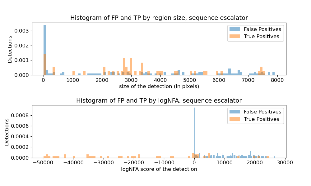
Figure 5: Comparison of the histograms of TP and FP computed by the BSUVFPM algorithm for the sequence escalator, by size of the detection (top) and by the $\log(\mathrm{NFA})$ score (bottom).

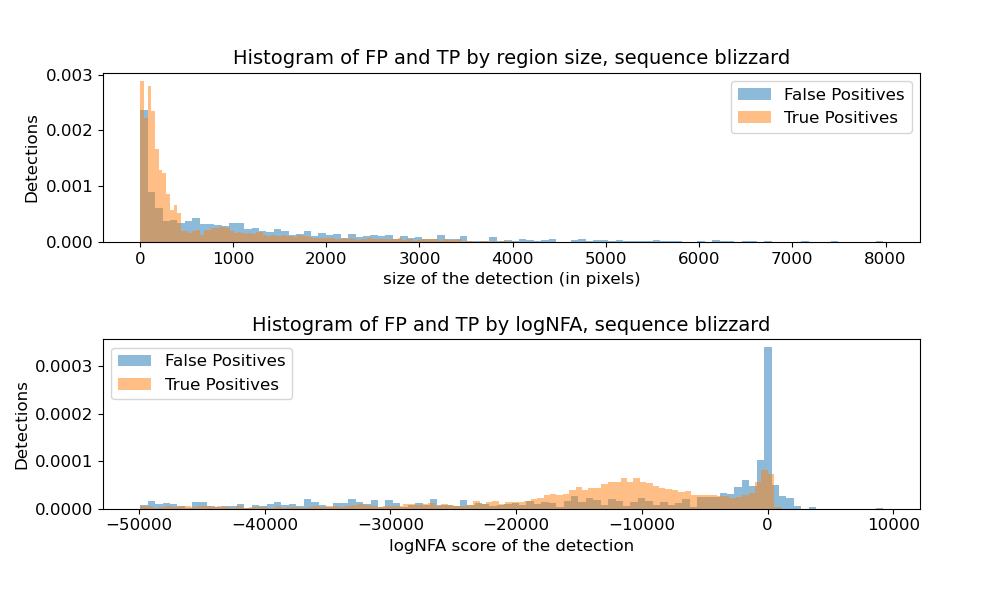
Figure 6: Comparison of the histograms of TP and FP computed by the SemanticBGS algorithm (with SuBSENSE) for the sequence blizzard, by size of the detection (top) and by the $\log(\mathrm{NFA})$ score (bottom).

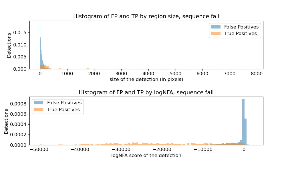
Figure 7: Comparison of the histograms of TP and FP computed by the SuBSENSE algorithm for the sequence fall, by size of the detection (top) and by the $\log(\mathrm{NFA})$ score (bottom).

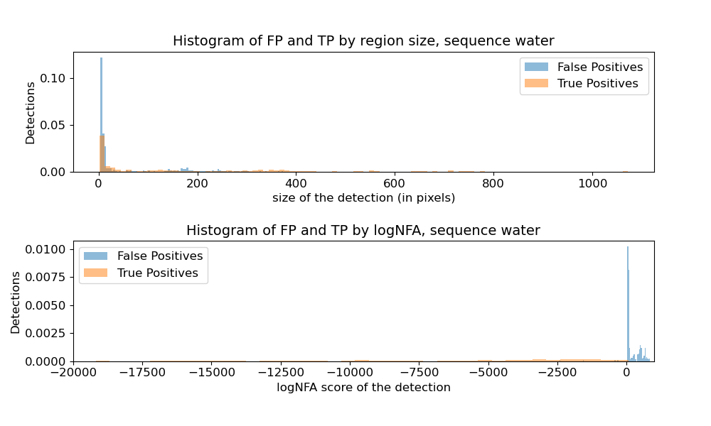
Figure 8: Comparison of the histograms of TP and FP computed by the ViBe algorithm for the sequence water, by size of the detection (top) and by the $\log(\mathrm{NFA})$ score (bottom).

References

- [1] Aitor Artola, Yannis Kolodziej, Jean-Michel Morel, and Thibaud Ehret. Glad: A global-to-local anomaly detector. In 2023 IEEE Winter Conference on Applications of Computer Vision (WACV). IEEE, 2023.
- [2] Mohammadreza Babaee, Duc Tung Dinh, and Gerhard Rigoll. A deep convolutional neural network for background subtraction. CoRR, abs/1702.01731, 2017.
- [3] Adrien Bardes, Jean Ponce, and Yann LeCun. Vicreg: Variance-invariance-covariance regularization for self-supervised learning. CoRR, abs/2105.04906, 2021.
- [4] Olivier Barnich and Marc Van Droogenbroeck. Vibe: A universal background subtraction algorithm for video sequences. IEEE Transactions on Image Processing, 20(6):1709–1724, 2011.
- [5] Thierry Bouwmans, Sajid Javed, Maryam Sultana, and Soon Ki Jung. Deep neural network concepts for background subtraction:a systematic review and comparative evaluation. Neural Networks, 117:8–66, 2019.
- [6] Marc Braham, Sebastien Pierard, and Marc Van Droogenbroeck. Semantic background subtraction. In IEEE International Conference on Image Processing (ICIP), pages 4552–4556, Beijing, China, September 2017.
- [7] Marc Braham and Marc Van Droogenbroeck. Deep background subtraction with scene-specific convolutional neural networks. In 2016 International Conference on Systems, Signals and Image Processing (IWSSIP), pages 1–4, 2016.
- [8] Robin Chan, Krzysztof Lis, Svenja Uhlemeyer, Hermann Blum, Sina Honari, Roland Siegwart, Pascal Fua, Mathieu Salzmann, and Matthias Rottmann. Segmentmeifyoucan: A benchmark for anomaly segmentation. arXiv preprint arXiv:2104.14812, 2021.
- [9] Anthony Cioppa, Marc Van Droogenbroeck, and Marc Braham. Real-time semantic background subtraction. In 2020 IEEE International Conference on Image Processing (ICIP), pages 3214–3218, 2020.
- [10] Carlos Cuevas, Eva María Yáñez, and Narciso García. Labeled dataset for integral evaluation of moving object detection algorithms: Lasiesta. Computer Vision and Image Understanding, 152:103–117, 2016.
- [11] Thomas Defard, Aleksandr Setkov, Angelique Loesch, and Romaric Audigier. Padim: a patch distribution modeling framework for anomaly detection and localization. In International Conference on Pattern Recognition, pages 475–489. Springer, 2021.
- [12] Agnès Delsolneux, Lionel Moisan, and Jean-Michel Morel. From Gestalt Theory to Image Analysis: A Probabilistic Approach, volume 34. Springer Science & Business Media, 2008.
- [13] Jia Deng, Wei Dong, Richard Socher, Li-Jia Li, Kai Li, and Li Fei-Fei. Imagenet: A large-scale hierarchical image database. In 2009 IEEE Conference on Computer Vision and Pattern Recognition, pages 248–255, 2009.
- [14] Agnès Desolneux, Lionel Moisan, and Jean-Michel Morel. Meaningful alignments. International Journal of Computer Vision, 40:7–23, 2000.
- [15] Belmar Garcia-Garcia, Thierry Bouwmans, and Alberto Jorge Rosales Silva. Background subtraction in real applications: Challenges, current models and future directions. Computer Science Review, 35:100204, 2020.
- [16] Hadi Ghahremannezhad, Hang Shi, and Chengjun Liu. Real-time hysteresis foreground detection in video captured by moving cameras. In 2022 IEEE International Conference on Imaging Systems and Techniques (IST), pages 1–6, 2022.
- [17] Solomon W. Golomb. Polyominoes: Puzzles, Patterns, Problems, and Packings - Revised and Expanded Second Edition. Princeton University Press, 2020.
- [18] Alexander Gordon, Galina Glazko, Xing Qiu, and Andrei Yakovlev. Control of the mean number of false discoveries, bonferroni and stability of multiple testing. The Annals of Applied Statistics, 1, 2007.
- [19] Nil Goyette, Pierre-Marc Jodoin, Fatih Porikli, Janusz Konrad, and Prakash Ishwar. Changedetection. net: A new change detection benchmark dataset. In 2012 IEEE computer society conference on computer vision and pattern recognition workshops, pages 1–8. IEEE, 2012.
- [20] Rafael Grompone, Charles Hessel, Tristan Dagobert, Jean-Michel Morel, and Carlo de Franchis. Ground visibility in satellite optical time series based on a contrario local image matching. Image Processing On Line, 11:212–233, 2021.
- [21] Michael Harville. A framework for high-level feedback to adaptive, per-pixel, mixture-of-gaussian background models. In Anders Heyden, Gunnar Sparr, Mads Nielsen, and Peter Johansen, editors, Computer Vision — ECCV 2002, pages 543–560, Berlin, Heidelberg, 2002. Springer Berlin Heidelberg.
- [22] Kaiming He, Xiangyu Zhang, Shaoqing Ren, and Jian Sun. Deep residual learning for image recognition. In 2016 IEEE Conference on Computer Vision and Pattern Recognition (CVPR), pages 770–778, 2016.
- [23] Tatsuya Ishikawa and Thi Thi Zin. A Study on Detection of Suspicious Persons for Intelligent Monitoring System, pages 292–301. Springer, 2019.
- [24] Iwan Jensen and Anthony J Guttmann. Statistics of lattice animals (polyominoes) and polygons. Journal of Physics A: Mathematical and General, 33(29):L257, 2000.
- [25] Long Ang Lim and Hacer Keles. Foreground segmentation using a triplet convolutional neural network for multiscale feature encoding. Pattern Recognition Letters, 112, 2018.
- [26] Jose-Luis Lisani and Silvia Ramis. A contrario detection of faces with a short cascade of classifiers. Image Processing On Line, 9:269–290, 2019.
- [27] David G. Lowe. Perceptual Organization and Visual Recognition. Kluwer Academic Publishers, 1985.
- [28] Khrystyna Lyubymenko, Milan Adamek, and Lukas Kralik. Detection of suspicious persons and special software. In 2017 12th Iberian Conference on Information Systems and Technologies (CISTI), pages 1–4, 2017.
- [29] Matthias Michael, Christian Feist, Florian Schuller, and Marc Tschentscher. Fast change detection for camera-based surveillance systems. In 2016 IEEE 19th International Conference on Intelligent Transportation Systems (ITSC), pages 2481–2486, 2016.
- [30] Anurag Mittal and Dan Huttenlocher. Scene modeling for wide area surveillance and image synthesis. In Proceedings IEEE Conference on Computer Vision and Pattern Recognition. CVPR 2000 (Cat. No.PR00662), volume 2, pages 160–167 vol.2, 2000.
- [31] Hyeoncheol Noh, Jingi Ju, Minseok Seo, Jongchan Park, and Dong-Geol Choi. Unsupervised change detection based on image reconstruction loss. In Proceedings of the IEEE/CVF Conference on Computer Vision and Pattern Recognition, pages 1352–1361, 2022.
- [32] Elyes Ouerghi, Thibaud Ehret, Carlo de Franchis, Gabriele Facciolo, Thomas Lauvaux, Enric Meinhardt, and Jean-Michel Morel. Detection of methane plumes in hyperspectral images from sentinel-5p by coupling anomaly detection and pattern recognition. ISPRS Annals of the Photogrammetry, Remote Sensing and Spatial Information Sciences, V-3-2021:81–87, 2021.
- [33] Elyes Ouerghi, Thibaud Ehret, Carlo de Franchis, Gabriele Facciolo, Thomas Lauvaux, Enric Meinhardt, and Jean-Michel Morel. Automatic methane plumes detection in time series of sentinel-5p l1b images. ISPRS Annals of the Photogrammetry, Remote Sensing and Spatial Information Sciences, V-3-2022:147–154, 2022.
- [34] Behnaz Rezaei, Amirreza Farnoosh, and Sarah Ostadabbas. G-lbm: Generative low-dimensional background model estimation from video sequences. In European Conference on Computer Vision, pages 293–310. Springer, 2020.
- [35] Amandine Robin, Lionel Moisan, and Sylvie Le Hegarat-Mascle. An a-contrario approach for subpixel change detection in satellite imagery. IEEE Transactions on Pattern Analysis and Machine Intelligence, 32(11):1977–1993, 2010.
- [36] Matthias Rottmann, Pascal Colling, Thomas Paul Hack, Robin Chan, Fabian Hüger, Peter Schlicht, and Hanno Gottschalk. Prediction error meta classification in semantic segmentation: Detection via aggregated dispersion measures of softmax probabilities. In 2020 International Joint Conference on Neural Networks (IJCNN), pages 1–9. IEEE, 2020.
- [37] Dimitrios Sakkos, Heng Liu, Jungong Han, and Ling Shao. End-to-end video background subtraction with 3d convolutional neural networks. Multimedia Tools and Applications, 77, 2018.
- [38] Imran Saleemi, Lance Hartung, and Mubarak Shah. Scene understanding by statistical modeling of motion patterns. In 2010 IEEE Computer Society Conference on Computer Vision and Pattern Recognition, pages 2069–2076, 2010.
- [39] Karen Simonyan and Andrew Zisserman. Very deep convolutional networks for large-scale image recognition. arXiv 1409.1556, 2014.
- [40] Andrews Sobral and Antoine Vacavant. A comprehensive review of background subtraction algorithms evaluated with synthetic and real videos. Computer Vision and Image Understanding, 122:4–21, 2014.
- [41] Pierre-Luc St-Charles, Guillaume-Alexandre Bilodeau, and Robert Bergevin. Subsense: A universal change detection method with local adaptive sensitivity. IEEE Transactions on Image Processing, 24(1):359–373, 2015.
- [42] Chris Stauffer and W.E.L. Grimson. Adaptive background mixture models for real-time tracking. In Proceedings. 1999 IEEE Computer Society Conference on Computer Vision and Pattern Recognition (Cat. No PR00149), volume 2, pages 246–252 Vol. 2, 1999.
- [43] Mustafa Ozan Tezcan, Prakash Ishwar, and Janusz Konrad. Bsuv-net: A fully-convolutional neural network for background subtraction of unseen videos. In 2020 IEEE Winter Conference on Applications of Computer Vision (WACV), pages 2763–2772, 2020.
- [44] Mustafa Ozan Tezcan, Prakash Ishwar, and Janusz Konrad. Bsuv-net 2.0: Spatio-temporal data augmentations for video-agnostic supervised background subtraction. IEEE Access, PP:1–1, 04 2021.
- [45] Yi Wang, Pierre-Marc Jodoin, Fatih Porikli, Janusz Konrad, Yannick Benezeth, and Prakash Ishwar. Cdnet 2014: An expanded change detection benchmark dataset. In Proceedings of the IEEE conference on computer vision and pattern recognition workshops, pages 387–394, 2014.
- [46] Andrew P. Witkin and Jay M. Tenenbaum. On the role of structure in vision. In Jacob Beck, Barbara Hope, and Azriel Rosenfeld, editors, Human and Machine Vision, Notes and Reports in Computer Science and Applied Mathematics, pages 481–543. Academic Press, 1983.
- [47] Jing Zhong and Stan Sclaroff. Segmenting foreground objects from a dynamic textured background via a robust kalman filter. In Proceedings Ninth IEEE International Conference on Computer Vision, pages 44–50 vol.1, 2003.
- [48] Zoran Zivkovic. Improved adaptive gaussian mixture model for background subtraction. In Proceedings of the 17th International Conference on Pattern Recognition, 2004. ICPR 2004., volume 2, pages 28–31 Vol.2, 2004.