Well posedness of fluid-solid mixture models for biofilm spread

Ana Carpio (Universidad Complutense de Madrid),
Gema Duro (Universidad Autรณnoma de Madrid)

Abstract Two phase solid-fluid mixture models are ubiquitous in biological applications. For instance, models for growth of tissues and biofilms combine time dependent and quasi-stationary boundary value problems set in domains whose boundary moves in response to variations in the mechano-chemical variables. For a model of biofilm spread, we show how to obtain better posed models by characterizing the time derivatives of relevant quasi-stationary magnitudes in terms of additional boundary value problems. We also give conditions for well posedness of time dependent submodels set in moving domains depending on the motion of the boundary. After constructing solutions for transport, diffusion and elliptic submodels for volume fractions, displacements, velocities, pressures and concentrations with the required regularity, we are able to handle the full model of biofilm spread in moving domains assuming we know the dynamics of the boundary. These techniques are general and can be applied in models with a similar structure arising in biological and chemical engineering applications.

Keyword. Fluid-solid mixture models, thin film approximations, evolution equations in moving domains, quasi-stationary approximations, stationary transport equations.

1 Introduction

Biofilms are bacterial aggregates that adhere to moist surfaces. Bacteria are encased in a self-produced polymeric matrix [13] which shelters them from chemical and mechanical aggressions. Biofilms formed on medical equipment, such as implants and catheters, are responsible for hospital-acquired infections [28]. In industrial environments, they cause substantial economical and technical problems, associated to food poisoning, biofouling, biocorrosion, contaminated ventilation systems, and so on [10, 22, 29]. Modeling biofilm spread is important to be able to eradicate them.

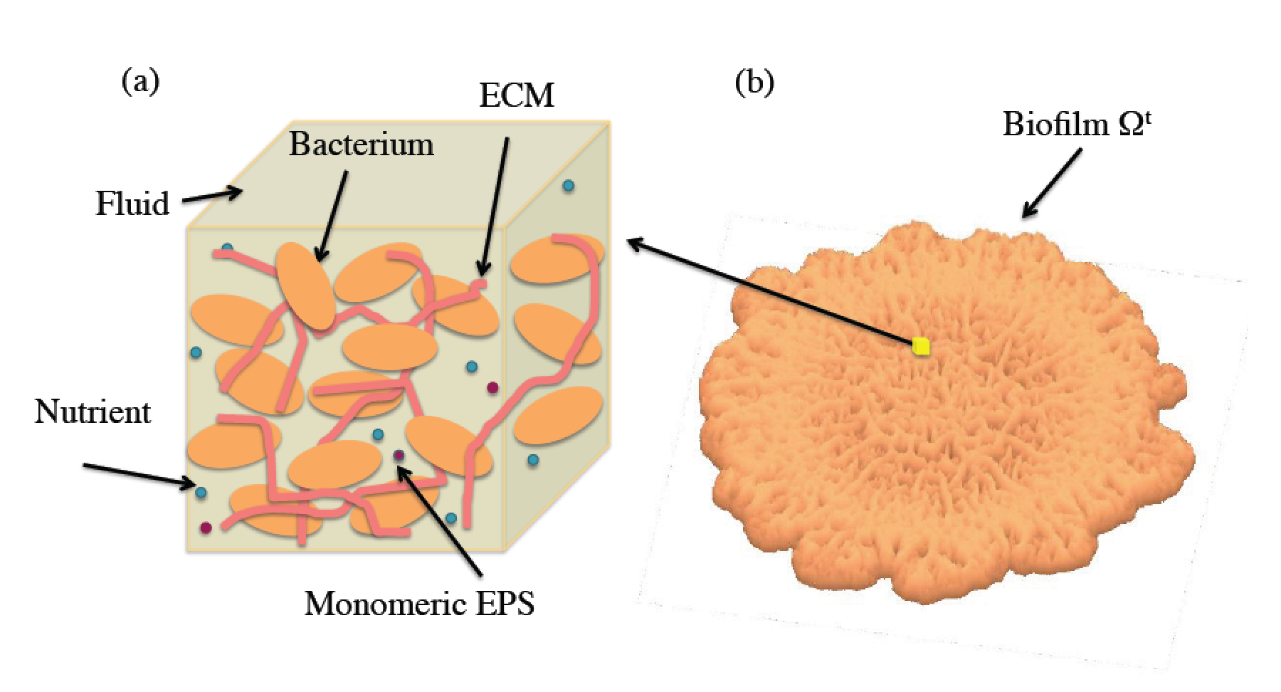
We describe here biofilms in terms of solid-fluid mixtures, see Figure 1. At each point $\mathbf{x}$ of the biofilm we have a solid fraction of biomass ฯ•sโ€‹(๐ฑ,t)subscriptitalic-ฯ•๐‘ ๐ฑ๐‘ก\phi_{s}(\mathbf{x},t) (cell biomass, polymeric threads) and a volume fraction of water $\phi_{f}(\mathbf{x},t)$ containing dissolved substances (nutrients, autoinducers and so on), in such a way that ฯ•sโ€‹(๐ฑ,t)+ฯ•fโ€‹(๐ฑ,t)=1.subscriptitalic-ฯ•๐‘ ๐ฑ๐‘กsubscriptitalic-ฯ•๐‘“๐ฑ๐‘ก1\phi_{s}(\mathbf{x},t)+\phi_{f}(\mathbf{x},t)=1. The solid and fluid volume fractions move with velocities ๐ฏssubscript๐ฏ๐‘ \mathbf{v}_{s} and $\mathbf{v}_{f}$, respectively.

Refer to caption
Figure 1: (a) Schematic view of biofilm microscopic structure. Cells are embedded in a network of polymeric threads forming the extracellular matrix (ECM), while a liquid solution containing nutrients and chemicals flows through the network. (b) Schematic view of a biofilm spreading on a surface.
Refer to caption
Refer to caption
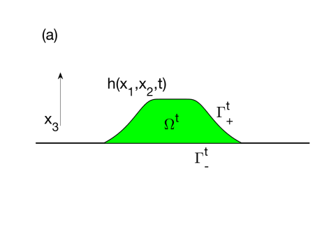
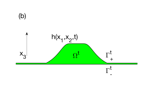
Figure 2: Schematic representation of a biofilm slice $\Omega^{t}$ spreading on a surface (a) occupying a finite region and ending at triple contact points, (b) spreading over precursor layers. The upper boundary $\Gamma^{t}_{+}$ represents the biofilm/air interface. The lower boundary $\Gamma^{t}_{-}$ represents the biofilm/agar interface, which provides nutrients and resources necessary for biofilm growth in our framework.

Biofilm spread on an air/solid interface is governed by the following system of equations, see [7, 18]. Assume a biofilm occupies a region $\Omega^{t}$, that varies with time. Figure 2 represents schematic views of two dimensional slices. The upper boundary $\Gamma^{t}_{+}$ separates the biofilm from an outer fluid, that can be a liquid or air. A lower boundary $\Gamma^{t}_{-}$ separates the biofilm from the substratum it attaches to. The main variables satisfy a set of quasi-stationary equations

$\displaystyle\begin{array}[]{lcl}\displaystyle{\rm div}({\mathbf{v}}_{f}\phi_{f})&=&-k_{s}{c\over c+K_{s}}\phi_{s},\\[4.30554pt] \displaystyle{\rm div}(k_{h}(\phi_{s})\nabla(p-\pi(\phi_{s}))&=&{\rm div}(\mathbf{v}_{s}),\\[4.30554pt] \displaystyle\mu\Delta\mathbf{u}_{s}+(\mu+\lambda)\nabla({\rm div}(\mathbf{u}_{s}))&=&\nabla p,\\[4.30554pt] \displaystyle-d\Delta c+{\rm div}(\mathbf{v}_{f}c)&=&-k_{c}{c\over c+K_{c}}\phi_{s},\end{array}$ (5)

constrained by the additional conditions

ฯ•fโ€‹๐ฏf=โˆ’khโ€‹(ฯ•s)โ€‹โˆ‡(pโˆ’ฯ€โ€‹(ฯ•s))+ฯ•fโ€‹๐ฏs,๐ฏs=โˆ‚๐ฎsโˆ‚t,ฯ•f+ฯ•s=1,formulae-sequencesubscriptitalic-ฯ•๐‘“subscript๐ฏ๐‘“subscript๐‘˜โ„Žsubscriptitalic-ฯ•๐‘ โˆ‡๐‘๐œ‹subscriptitalic-ฯ•๐‘ subscriptitalic-ฯ•๐‘“subscript๐ฏ๐‘ formulae-sequencesubscript๐ฏ๐‘ subscript๐ฎ๐‘ ๐‘กsubscriptitalic-ฯ•๐‘“subscriptitalic-ฯ•๐‘ 1\displaystyle\phi_{f}\mathbf{v}_{f}=-k_{h}(\phi_{s})\nabla(p-\pi(\phi_{s}))+\phi_{f}\mathbf{v}_{s},\quad{\mathbf{v}_{s}}={\partial\mathbf{u}_{s}\over\partial t},\quad\phi_{f}+\phi_{s}=1, (6)

in the region occupied by the biofilm $\Omega^{t}$, which varies with time. In this quasi-static framework, the displacement vector ๐ฎsโ€‹(๐ฑ,t)subscript๐ฎ๐‘ ๐ฑ๐‘ก\mathbf{u}_{s}(\mathbf{x},t) and the scalar pressure $p(\mathbf{x},t)$, volume fraction ฯ•sโ€‹(๐ฑ,t)subscriptitalic-ฯ•๐‘ ๐ฑ๐‘ก\phi_{s}(\mathbf{x},t) and concentration $c(\mathbf{x},t)$ fields depend on time through variations of the boundary $\Gamma^{t}$, which expands due to cell division and swelling. The positive functions khโ€‹(ฯ•s)subscript๐‘˜โ„Žsubscriptitalic-ฯ•๐‘ k_{h}(\phi_{s}) and ฯ€โ€‹(ฯ•s)๐œ‹subscriptitalic-ฯ•๐‘ \pi(\phi_{s}) represent the permeability and the osmotic pressure. This system is subject to a set of boundary conditions:

pโˆ’ฯ€=peโ€‹xโ€‹tโˆ’ฯ€eโ€‹xโ€‹t,onย โ€‹ฮ“t=ฮ“+tโˆชฮ“โˆ’t,(๐ˆ^โ€‹(๐ฎs)โˆ’pโ€‹๐ˆ)โ€‹๐ง=๐ญeโ€‹xโ€‹t,โˆ‚cโˆ‚๐ง=0,onย โ€‹ฮ“+t,๐ฎs=0,c=c0,onย โ€‹ฮ“โˆ’t,๐‘๐œ‹subscript๐‘๐‘’๐‘ฅ๐‘กsubscript๐œ‹๐‘’๐‘ฅ๐‘กonย superscriptฮ“๐‘กsubscriptsuperscriptฮ“๐‘กsubscriptsuperscriptฮ“๐‘กformulae-sequence^๐ˆsubscript๐ฎ๐‘ ๐‘๐ˆ๐งsubscript๐ญ๐‘’๐‘ฅ๐‘ก๐‘๐ง0onย subscriptsuperscriptฮ“๐‘กformulae-sequencesubscript๐ฎ๐‘ 0๐‘subscript๐‘0onย subscriptsuperscriptฮ“๐‘ก\displaystyle\begin{array}[]{ll}\displaystyle p-\pi=p_{ext}-\pi_{ext},&\qquad\mbox{on }\Gamma^{t}=\Gamma^{t}_{+}\cup\Gamma^{t}_{-},\\ \displaystyle(\hat{\boldsymbol{\sigma}}(\mathbf{u}_{s})-p\mathbf{I})\mathbf{n}=\mathbf{t}_{ext},\;{\partial c\over\partial\mathbf{n}}=0,&\qquad\mbox{on }\Gamma^{t}_{+},\\[4.30554pt] \displaystyle\mathbf{u}_{s}=0,\;c=c_{0},&\qquad\mbox{on }\Gamma^{t}_{-},\end{array} (10)

where $\mathbf{n}$ is the outer unit normal and

๐ˆ^โ€‹(๐ฎs)=ฮปโ€‹Trโ€‹(๐œบโ€‹(๐ฎs))โ€‹๐ˆ+2โ€‹ฮผโ€‹๐œบโ€‹(๐ฎs),ฮตiโ€‹jโ€‹(๐ฎ)=12โ€‹(โˆ‚uiโˆ‚xj+โˆ‚ujโˆ‚xi),i,j=1,โ€ฆ,n,formulae-sequence^๐ˆsubscript๐ฎ๐‘ ๐œ†Tr๐œบsubscript๐ฎ๐‘ ๐ˆ2๐œ‡๐œบsubscript๐ฎ๐‘ formulae-sequencesubscript๐œ€๐‘–๐‘—๐ฎ12subscript๐‘ข๐‘–subscript๐‘ฅ๐‘—subscript๐‘ข๐‘—subscript๐‘ฅ๐‘–๐‘–๐‘—1โ€ฆ๐‘›\hat{\boldsymbol{\sigma}}(\mathbf{u}_{s})=\lambda{\rm Tr}(\boldsymbol{\varepsilon}({\mathbf{u}}_{s}))\,\mathbf{I}+2\mu\,\boldsymbol{\varepsilon}({\mathbf{u}}_{s}),\quad\varepsilon_{ij}({\mathbf{u}})={1\over 2}\Big{(}{\partial u_{i}\over\partial x_{j}}+{\partial u_{j}\over\partial x_{i}}\Big{)},\;i,j=1,\ldots,n,

$n=2,3,$ represent elastic stress and strain tensors. Boundary conditions for $\phi_{f}$ are required or not depending on the sign of $\mathbf{v}_{f}\cdot\mathbf{n}$ at the border. The displacement and velocity vectors have components $\mathbf{u}=(u_{1},\ldots,u_{n})$ and $\mathbf{v}=(v_{1},\ldots,v_{n})$, $n=2,3$, respectively. All the parameters appearing in the model, kssubscript๐‘˜๐‘ k_{s}, Kssubscript๐พ๐‘ K_{s}, $k_{c}$, $K_{c}$, $\mu$, $\lambda$, $d$ are positive constants. For ease of the reader, we have summarized the modeling in Appendix A. In some limits, the system can be reformulated as a poroelastic model [8, 15].

The model is complemented with an equation for the dynamics of $\Gamma^{t}$, $t>0$. If we consider biofilms represented by the scheme in Figure 2(a), the contact points between biofilm, air and agar require specific additional information to avoid singularities. We will work with the geometry represented in Figure 2(b), that avoids this difficulty by introducing precursor layers [23, 12]. Then, $\Gamma^{t}_{-}$ is fixed. The upper boundary $\Gamma^{t}_{+}$ is parametrized by a height function $h(x_{1},x_{2},t)$, which satisfies the equation [7]

$\displaystyle{\partial h\over\partial t}+{\partial\over\partial x_{1}}\left[\int_{0}^{h}(\mathbf{v}\cdot\hat{\mathbf{x}}_{1})\,dx_{3}\right]+{\partial\over\partial x_{2}}\left[\int_{0}^{h}(\mathbf{v}\cdot\hat{\mathbf{x}}_{2})\,dx_{3}\right]=\mathbf{v}\cdot\hat{\mathbf{x}}_{3}\big{|}_{0},$ (11)

where the composite velocity of the mixture ๐ฏ=ฯ•fโ€‹๐ฏf+ฯ•sโ€‹๐ฏs๐ฏsubscriptitalic-ฯ•๐‘“subscript๐ฏ๐‘“subscriptitalic-ฯ•๐‘ subscript๐ฏ๐‘ \mathbf{v}=\phi_{f}\mathbf{v}_{f}+\phi_{s}\mathbf{v}_{s} has components ๐ฏโ‹…๐ฑ^i=vs,iโˆ’khโ€‹(ฯ•s)โ€‹โˆ‚(pโˆ’ฯ€)โˆ‚xi,i=1,2,3formulae-sequenceโ‹…๐ฏsubscript^๐ฑ๐‘–subscript๐‘ฃ๐‘ ๐‘–subscript๐‘˜โ„Žsubscriptitalic-ฯ•๐‘ ๐‘๐œ‹subscript๐‘ฅ๐‘–๐‘–123\mathbf{v}\cdot\hat{\mathbf{x}}_{i}=v_{s,i}-k_{h}(\phi_{s}){\partial(p-\pi)\over\partial x_{i}},i=1,2,3.

At present, only perturbation analyses and numerical studies are available for this type of models [7, 23] in simple geometries. Asymptotic studies yield thin film type approximations for (5)-(11) assuming circular geometries and radial symmetry. Non standard lubrication equations for the height $h$ are obtained, which admit families of self-similar solutions in radial geometries. However, the construction of reliable numerical solutions of the model in general experimental configurations faces difficulties due to the lack of well-posedness results.

In this paper, we assume we know the dynamics of the upper boundary $\Gamma_{+}^{t}$, given by a smooth curve $x_{3}=h(x_{1},x_{2},t)$, and develop an existence and stability theory for the model equations. To simplify the analysis, we take khโ€‹(ฯ•s)=kh>0subscript๐‘˜โ„Žsubscriptitalic-ฯ•๐‘ subscript๐‘˜โ„Ž0k_{h}(\phi_{s})=k_{h}>0, khโ€‹(ฯ•s)/ฯ•f=ฮพโˆž>0subscript๐‘˜โ„Žsubscriptitalic-ฯ•๐‘ subscriptitalic-ฯ•๐‘“subscript๐œ‰0k_{h}(\phi_{s})/\phi_{f}=\xi_{\infty}>0 and ฯ€โ€‹(ฯ•s)=ฮ โ€‹ฯ•s>0๐œ‹subscriptitalic-ฯ•๐‘ ฮ subscriptitalic-ฯ•๐‘ 0\pi(\phi_{s})=\Pi\phi_{s}>0. In this quasi-stationary framework, the displacements ๐ฎssubscript๐ฎ๐‘ \mathbf{u}_{s} depend on time through the motion of the boundary. However, we lack equations for the velocities, other than the relation โˆ‚๐ฎsโˆ‚t=๐ฏssubscript๐ฎ๐‘ ๐‘กsubscript๐ฏ๐‘ {\partial\mathbf{u}_{s}\over\partial t}=\mathbf{v}_{s}. In Section 2 we obtain a system of equations characterizing the velocity:

divโ€‹(๐ˆ^โ€‹(๐ฏs))=ฮผโ€‹ฮ”โ€‹๐ฏs+(ฮผ+ฮป)โ€‹โˆ‡(divโ€‹(๐ฏs))=โˆ‡pt,div^๐ˆsubscript๐ฏ๐‘ ๐œ‡ฮ”subscript๐ฏ๐‘ ๐œ‡๐œ†โˆ‡divsubscript๐ฏ๐‘ โˆ‡subscript๐‘๐‘ก\displaystyle{\rm div}(\hat{\boldsymbol{\sigma}}(\mathbf{v}_{s}))=\mu\Delta\mathbf{v}_{s}+(\mu+\lambda)\nabla({\rm div}(\mathbf{v}_{s}))=\nabla p_{t}, $\displaystyle\;\mbox{in $\Omega^{t}$},$
๐ฏs=0,subscript๐ฏ๐‘ 0\displaystyle\mathbf{v}_{s}=0, $\displaystyle\;\mbox{on $\Gamma_{-}^{t}$},$ (12)
๐ˆ^โ€‹(๐ฏs)โ€‹๐ง=โˆ‚๐ โˆ‚t+๐ซโ€‹(๐ ,๐ฎs),^๐ˆsubscript๐ฏ๐‘ ๐ง๐ ๐‘ก๐ซ๐ subscript๐ฎ๐‘ \displaystyle\hat{\boldsymbol{\sigma}}(\mathbf{v}_{s})\mathbf{n}={\partial\mathbf{g}\over\partial t}+\mathbf{r}(\mathbf{g},\mathbf{u}_{s}), on $\Gamma_{+}^{t}$,

with $g=-p\mathbf{n}=-(p_{\rm ext}-\pi_{\rm ext})\mathbf{n}$ and ${\mathbf{r}}$ to be defined later. A similar equation is obtained for $p_{t}$ from the equation for $p$. Taking the divergence of the equations for ๐ฎssubscript๐ฎ๐‘ \mathbf{u}_{s} and ๐ฏssubscript๐ฏ๐‘ \mathbf{v}_{s} we find additional equations to close the system

dโ€‹edโ€‹t=khโ€‹(2โ€‹ฮผ+ฮป)โ€‹ฮ”โ€‹eโˆ’khโ€‹ฮ โ€‹ฮ”โ€‹ฯ•s,๐‘‘๐‘’๐‘‘๐‘กsubscript๐‘˜โ„Ž2๐œ‡๐œ†ฮ”๐‘’subscript๐‘˜โ„Žฮ ฮ”subscriptitalic-ฯ•๐‘ \displaystyle{de\over dt}=k_{h}(2\mu+\lambda)\Delta e-k_{h}\Pi\Delta\phi_{s}, $\displaystyle\;\mbox{in $\Omega^{t}$},$ (13)
dโ€‹etdโ€‹t=khโ€‹(2โ€‹ฮผ+ฮป)โ€‹ฮ”โ€‹etโˆ’khโ€‹ฮ โ€‹ฮ”โ€‹ฯ•s,t,๐‘‘subscript๐‘’๐‘ก๐‘‘๐‘กsubscript๐‘˜โ„Ž2๐œ‡๐œ†ฮ”subscript๐‘’๐‘กsubscript๐‘˜โ„Žฮ ฮ”subscriptitalic-ฯ•๐‘ ๐‘ก\displaystyle{de_{t}\over dt}=k_{h}(2\mu+\lambda)\Delta e_{t}-k_{h}\Pi\Delta\phi_{s,t}, $\displaystyle\;\mbox{in $\Omega^{t}$},$ (14)

where e=divโ€‹(๐ฎs)๐‘’divsubscript๐ฎ๐‘ e={\rm div}(\mathbf{u}_{s}) and et=divโ€‹(๐ฏs)subscript๐‘’๐‘กdivsubscript๐ฏ๐‘ e_{t}={\rm div}(\mathbf{v}_{s}). We will neglect ฮ”โ€‹ฯ•s,tฮ”subscriptitalic-ฯ•๐‘ ๐‘ก\Delta\phi_{s,t} in (14) because ฮ ฮ \Pi and ฮ”โ€‹ฯ•sฮ”subscriptitalic-ฯ•๐‘ \Delta\phi_{s} are small compared to other terms. Notice that (13) and (14) are time dependent problems set in time dependent domains, while most results in the literature refer to fixed domains.

The construction of solutions for such systems combines a number of difficulties that we will address in stages. Section 2 characterizes the time derivatives of ๐ฎssubscript๐ฎ๐‘ \mathbf{u}_{s} and $p$, solutions of elliptic problems in time dependent domains, by means of additional boundary value problems. In this way we improve the stability of the model, since solving additional partial differential equations in each spatial domain is more effective than approximating time derivatives by quotients of differences of solutions calculated in variable spatial domains. Section 3 establishes well posedness results for linear parabolic problems (14) set in domains with moving boundaries for specific types of parametrizations. Section 4 considers the elliptic and stationary transport problems involved in the quasi-stationary submodels, separately and in fixed domains, under hypotheses motivated by asymptotic studies and numerical solutions. Finally, section 5 considers the full coupled time dependent problem and section 6 discusses our conclusions and open issues. A final appendix summarizes modeling details.

2 Differentiation of quasi-stationary problems

In the previous section, we have defined the velocity ๐ฏssubscript๐ฏ๐‘ \mathbf{v}_{s} as the time derivative of the displacement ๐ฎssubscript๐ฎ๐‘ \mathbf{u}_{s}. The change in time of ๐ฎssubscript๐ฎ๐‘ \mathbf{u}_{s} is due to the motion of the upper boundary $\Gamma^{t}_{+}$, that is, time variations in $h$. In this section we seek an equation characterizing ๐ฏssubscript๐ฏ๐‘ \mathbf{v}_{s}. We expect ๐ฏssubscript๐ฏ๐‘ \mathbf{v}_{s} to solve the same boundary value problem as ๐ฎssubscript๐ฎ๐‘ \mathbf{u}_{s}, but differentiating all sources with respect to time. However, since the boundary $\Gamma^{t}$ of $\Omega^{t}$ moves with time, we need to calculate the adequate boundary conditions too.

In the region $\Omega^{t}$ occupied by the moving biofilm, the displacements ๐ฎssubscript๐ฎ๐‘ \mathbf{u}_{s} of the solid phase satisfy equations (5) with boundary conditions (10). To simplify later computations, it is convenient to recast these equations in the general linear elasticity framework. The components of the displacement $u_{j}(t),j=1,\ldots,n$, $n$ being the dimension, fulfill

$\displaystyle-{\partial\over\partial x_{\alpha}}\left(c_{j\alpha m\beta}{\partial u_{m}(t)\over\partial x_{\beta}}\right)=f_{j}(t),\quad j=1,\ldots,n,$ $\displaystyle\qquad\mbox{in $\Omega^{t}$},$
$\displaystyle u_{j}(t)=0,\quad j=1,\ldots,n,$ $\displaystyle\qquad\mbox{on $\Gamma_{d}^{t}$},$ (15)
$\displaystyle\displaystyle c_{j\alpha m\beta}{\partial u_{m}(t)\over\partial x_{\beta}}n_{\alpha}(t)=g_{j}(t),\quad j=1,\ldots,n,$ on $\Gamma_{n}^{t}$,

where $\mathbf{n}(t)$ is the outer unit normal vector and $c_{j\alpha m\beta}$ the elastic constants. $\Gamma_{n}^{t}$ and $\Gamma_{d}^{t}$ are parts of the boundary $\Gamma^{t}$ where we enforce conditions on the stresses of the displacements, respectively.

We use the Einstein summation convention that implies summation over a set of indexed terms in a formula when repeated in it. In the above equations, summation over $\alpha,\beta,m$ is implied, but not over $j$. The elastic constants $c_{j\alpha m\beta}$ for a isotropic solids like the ones we consider are

$$c_{j\alpha m\beta}=\lambda\delta_{j\alpha}\delta_{m\beta}+\mu(\delta_{jm}\delta_{\alpha\beta}+\delta_{j\beta}\delta_{\alpha m})$$

where $\delta_{jm}$ stands for the Kronecker delta, whereas $\lambda$ and $\mu$ represent the Lamรฉ constants. The stress tensor is

$$\sigma_{j\alpha}=c_{j\alpha m\beta}\varepsilon_{m\beta}=\lambda\delta_{j\alpha}\varepsilon_{pp}+2\mu\varepsilon_{j\alpha}.$$

In this framework, the velocity $\mathbf{v}$ is the โ€˜Frรจchet derivativeโ€™ or โ€˜domain derivativeโ€™ of $\mathbf{u}$ with respect to $t$ [25], which is characterized by the solution of a boundary value problem, as we show next.

Theorem 2.1. We assume that the body $\mathbf{f}$ and boundary ๐ ๐ \mathbf{g} forces are differentiable in time, with values in $[L^{2}(\Omega^{t})]^{n}$ and $[L^{2}(\Gamma^{t})]^{n}$, respectively, with $t>0$, $n=2,3$ being the dimension. Moreover, the $C^{2}$ boundaries $\Gamma^{t}$ are obtained deforming $\Gamma^{0}$ along a smooth vector field $\boldsymbol{\nu}$. Then, the time derivative $\mathbf{v}(t)={\partial\mathbf{u}(t)\over\partial t}$, $t>0$, of the displacement given by (15) satisfies

$\displaystyle-{\partial\over\partial x_{\alpha}}\left(c_{j\alpha m\beta}{\partial v_{m}(t)\over\partial x_{\beta}}\right)={\partial f_{j}(t)\over\partial t},\quad j=1,..,n,$ $\displaystyle\quad\mathbf{x}\in\Omega^{t},$
$\displaystyle v_{j}(t)=0,\quad j=1,..,n,$ $\displaystyle\quad\mathbf{x}\in\Gamma_{d}^{t},$ (16)
$\displaystyle\displaystyle c_{j\alpha m\beta}{\partial v_{m}(t)\over\partial x_{\beta}}n_{\alpha}(t)={\partial g_{j}(t)\over\partial t}+r_{j}(g_{j}(t),\mathbf{u}(t)),\quad j=1,..,n,$ $\displaystyle\quad\mathbf{x}\in\Gamma_{n}^{t},$

where

$\displaystyle\begin{array}[]{l}\displaystyle r_{j}=c_{j\alpha m\beta}{\partial u_{m}(t)\over\partial x_{\beta}}{\partial\nu_{q}\over\partial x_{\alpha}}n_{q}(t)+c_{j\alpha m\beta}{\partial u_{m}(t)\over\partial x_{\beta}}{\partial(\nu_{p}n_{\alpha}(t))\over\partial x_{p}}\\[4.30554pt] \displaystyle\hskip 14.22636pt+c_{j\alpha m\beta}{\partial u_{m}(t)\over\partial x_{\beta}}{\partial\nu_{p}\over\partial x_{p}}n_{\alpha}(t)-g_{j}(t)\mathbf{n}(t)^{T}\nabla\boldsymbol{\nu}\,\mathbf{n}(t),\quad j=1,\ldots,n.\end{array}$ (19)

As a corollary, we get the expressions of interest for our model.

Corollary 2.2. Under the previous hypotheses, the time derivative ๐ฏsโ€‹(t)subscript๐ฏ๐‘ ๐‘ก\mathbf{v}_{s}(t), $t>0$, of the solution ๐ฎssubscript๐ฎ๐‘ \mathbf{u}_{s} of (5) with boundary conditions (10) satisfies

divโ€‹(๐ˆ^โ€‹(๐ฏs))=ฮผโ€‹ฮ”โ€‹๐ฏs+(ฮผ+ฮป)โ€‹โˆ‡(divโ€‹(๐ฏs))=โˆ‡pt,div^๐ˆsubscript๐ฏ๐‘ ๐œ‡ฮ”subscript๐ฏ๐‘ ๐œ‡๐œ†โˆ‡divsubscript๐ฏ๐‘ โˆ‡subscript๐‘๐‘ก\displaystyle{\rm div}(\hat{\boldsymbol{\sigma}}(\mathbf{v}_{s}))=\mu\Delta\mathbf{v}_{s}+(\mu+\lambda)\nabla({\rm div}(\mathbf{v}_{s}))=\nabla p_{t}, $\displaystyle\;\mathbf{x}\in\Omega^{t},$
๐ฏs=0,subscript๐ฏ๐‘ 0\displaystyle\mathbf{v}_{s}=0, $\displaystyle\;\mathbf{x}\in\Gamma_{-}^{t},$ (20)
๐ˆ^โ€‹(๐ฏs)โ€‹๐ง=โˆ‚gjโˆ‚t+rjโ€‹(gj,๐ฎs),j=1,2formulae-sequence^๐ˆsubscript๐ฏ๐‘ ๐งsubscript๐‘”๐‘—๐‘กsubscript๐‘Ÿ๐‘—subscript๐‘”๐‘—subscript๐ฎ๐‘ ๐‘—12\displaystyle\hat{\boldsymbol{\sigma}}(\mathbf{v}_{s})\mathbf{n}={\partial g_{j}\over\partial t}+r_{j}(g_{j},\mathbf{u}_{s}),\;j=1,2 $\displaystyle\;\mathbf{x}\in\Gamma_{+}^{t},$

with $g=-p\mathbf{n}=-(p_{\rm ext}-\pi_{\rm ext})\mathbf{n}$ and ${\mathbf{r}}$ is defined by (19) with $c_{j\alpha m\beta}=\lambda\delta_{j\alpha}\delta_{m\beta}+\mu(\delta_{jm}\delta_{\alpha\beta}+\delta_{j\beta}\delta_{\alpha m}).$

Corollary 2.3 Under the previous hypotheses, assuming kkโ€‹(ฯ•s)=khsubscript๐‘˜๐‘˜subscriptitalic-ฯ•๐‘ subscript๐‘˜โ„Žk_{k}(\phi_{s})=k_{h} and ฯ€โ€‹(ฯ•s)=ฮ โ€‹ฯ•s๐œ‹subscriptitalic-ฯ•๐‘ ฮ subscriptitalic-ฯ•๐‘ \pi(\phi_{s})=\Pi\phi_{s}, the derivative $p_{t}(t)={\partial p(t)\over\partial t}$, $t>0,$ of the solution $p$ of (5) with Dirichlet boundary conditions $p=p_{ext}(t)$ satisfies,

khโ€‹ฮ”โ€‹pt=divโ€‹(๐ฏs,t)+khโ€‹ฮ โ€‹ฮ”โ€‹ฯ•s,t+,๐ฑโˆˆฮฉt,pt=pextโ€ฒโ€‹(t),๐ฑโˆˆฮ“t.subscript๐‘˜โ„Žฮ”subscript๐‘๐‘กdivsubscript๐ฏ๐‘ ๐‘กlimit-fromsubscript๐‘˜โ„Žฮ ฮ”subscriptitalic-ฯ•๐‘ ๐‘ก๐ฑsuperscriptฮฉ๐‘กsubscript๐‘๐‘กsuperscriptsubscript๐‘extโ€ฒ๐‘ก๐ฑsuperscriptฮ“๐‘ก\displaystyle\begin{array}[]{ll}k_{h}\Delta p_{t}={\rm div}(\mathbf{v}_{s,t})+k_{h}\Pi\Delta\phi_{s,t}+,&\mathbf{x}\in\Omega^{t},\\[4.30554pt] p_{t}=p_{\rm ext}^{\prime}(t),&\mathbf{x}\in\Gamma^{t}.\end{array} (22)

Proof of Theorem 2.1. We will follow a similar variational approach to that employed in [25] for 2D exterior elasticity problems with zero Dirichlet boundary conditions on a moving boundary. We are going to calculate the derivative at $t=0$. Similar arguments hold for any $t>0$.

Step 1: Variational formulation. First, we write the boundary value problem for $\mathbf{u}$ in variational form [21]. The boundary value problem (15) becomes: Find $\mathbf{u}^{t}\in[H^{1}_{\Gamma_{d}^{t}}(\Omega^{t})]^{n}$ such that

$$\displaystyle b^{t}(\Omega^{t};\mathbf{u}^{t},\mathbf{w}^{t})={\ell}^{t}(\Omega^{t};\mathbf{w}^{t}),\qquad\forall\,\mathbf{w}^{t}\in[H^{1}_{\Gamma_{d}^{t}}(\Omega^{t})]^{n},$$ (23)

where

$\displaystyle b^{t}(\Omega^{t};\mathbf{u}^{t},\mathbf{w}^{t})=\int_{\Omega^{t}}c_{j\alpha m\beta}{\partial u_{m}^{t}\over\partial x_{\beta}^{t}}{\partial\overline{w}_{j}^{t}\over\partial x_{\alpha}^{t}}\,d\mathbf{x}^{t},\qquad\forall\,\mathbf{u}^{t},\,\mathbf{w}^{t}\in[H^{1}_{\Gamma_{d}^{t}}(\Omega^{t})]^{n},$ (24)
$\displaystyle\ell^{t}(\Omega^{t};\mathbf{w}^{t})=\int_{\Omega^{t}}f_{j}(t)w_{j}^{t}\,d\mathbf{x}^{t}+\int_{\Gamma_{n}^{t}}g_{j}(t)w_{j}^{t}\,d\mathbf{S}_{\mathbf{x}^{t}},\qquad\forall\,\mathbf{w}^{t}\in[H^{1}_{\Gamma_{d}^{t}}(\Omega^{t})]^{n}.$ (25)

Here, $H^{1}_{\Gamma_{d}^{t}}(\Omega^{t})$ denotes the usual Sobolev space of $H^{1}(\Omega^{t})$ functions vanishing on $\Gamma_{d}^{t}\subset\partial\Omega^{t}$. $H^{1}(\Omega^{t})$ if formed by all functions whose square, and the squares of their derivatives, are integrable in $\Omega^{t}$, that is, belong to $L^{2}(\Omega^{t}).$ When $\mathbf{f}(t)\in[L^{2}(\Omega^{t})]^{n}$, ๐ โˆˆ[L2โ€‹(ฮ“t)]n๐ superscriptdelimited-[]superscript๐ฟ2superscriptฮ“๐‘ก๐‘›\mathbf{g}\in[L^{2}(\Gamma^{t})]^{n} and measโ€‹(ฮ“dt)โ‰ 0meassuperscriptsubscriptฮ“๐‘‘๐‘ก0{\rm meas}(\Gamma_{d}^{t})\neq 0, this problem admits a unique solution $\mathbf{u}^{t}\in[H^{1}_{\Gamma_{d}^{t}}(\Omega^{t})]^{n}$ [21], which in fact belongs to $[H^{2}(\Omega^{t})]^{n}$, vanishes on ${\Gamma_{d}^{t}}$ and satisfies ๐ˆโ€‹(๐ฎt)โ€‹๐ง=๐ ๐ˆsuperscript๐ฎ๐‘ก๐ง๐ \boldsymbol{\sigma}(\mathbf{u}^{t})\,\mathbf{n}=\mathbf{g} on $\Gamma_{n}^{t}=\partial\Omega^{t}\setminus\Gamma_{d}^{t}.$ For $t=0$, we have $u^{0}.$ Here, $\sigma_{\alpha j}(\mathbf{u}^{t})=c_{j\alpha m\beta}{\partial u_{m}^{t}\over\partial x_{\beta}}.$

Step 2: Change of variables. We now transform all the quantities appearing in (24)-(25) back to the initial configuration $\Omega^{0}$. The process is similar to transforming deformed configurations back to a reference configuration in continuum mechanics [14]. We are assumig that the evolution of the moving part of the boundary $\Gamma^{t}=\left\{\mathbf{x}+t\,\boldsymbol{\nu}(\mathbf{x})\,|\,\mathbf{x}\in\Gamma^{0}\right\}$ is given by a family of deformations $\mathbf{x}^{t}=\phi^{t}(\mathbf{x})=\mathbf{x}+t\,\boldsymbol{\nu}(\mathbf{x})$ starting from a smooth surface $\Gamma^{0}\in C^{2}$ (twice differentiable) and following a smooth vector field $\boldsymbol{\nu}\in C^{2}(\Omega)$, $\Omega^{t}\subset\Omega$, $t>0$. The deformation gradient is the jacobian of the change of variables [24]

$\displaystyle\mathbf{J}^{t}(\mathbf{x})=\nabla_{\mathbf{x}}\boldsymbol{\phi}^{t}(\mathbf{x})=\left({\partial x^{t}_{i}\over\partial x_{j}}(\mathbf{x})\right)=\mathbf{I}+t\,\nabla\boldsymbol{\nu}(\mathbf{x}),$ (26)

and its inverse $(\mathbf{J}^{t})^{-1}=\left({\partial x_{i}\over\partial x^{t}_{j}}\right)$ is the jacobian of the inverse change of variables. Then, volume and surface elements are related by

$\displaystyle d\mathbf{x}^{t}={\rm det}\,\mathbf{J}^{t}(\mathbf{x})\,d\mathbf{x},\quad dS_{\mathbf{x}^{t}}={\rm det}\,\mathbf{J}^{t}(\mathbf{x})\|\,(\mathbf{J}^{t}(\mathbf{x}))^{-T}\mathbf{n}\|dS_{\mathbf{x}}$ (27)

and the chain rule for derivatives reads $\nabla_{\mathbf{x}}u_{m}(\mathbf{x}^{t}(\mathbf{x}))=\mathbf{(}J^{t}(\mathbf{x}))^{T}\nabla_{\mathbf{x}^{t}}u_{m}(\mathbf{x}^{t}(\mathbf{x})),$ that is, $\nabla_{\mathbf{x}^{t}}u_{m}=(\mathbf{J}^{t})^{-T}\nabla_{\mathbf{x}}u_{m}$. For each component we have

$\displaystyle{\partial u_{m}\over\partial x_{\beta}^{t}}(\mathbf{x}^{t}(\mathbf{x}))={\partial u_{m}\over\partial x_{k}}(\mathbf{x}^{t}(\mathbf{x}))(J^{t})^{-1}_{k\beta}(\mathbf{x}).$ (28)

We define $\tilde{\mathbf{u}}(\mathbf{x})=\mathbf{u}^{t}\circ\phi^{t}(\mathbf{x})=\mathbf{u}^{t}(\mathbf{x}^{t}(\mathbf{x}))$, definition that extends to $\tilde{\mathbf{w}}$ and other functions. Changing variables and using (27)-(28) we have:

$\displaystyle b^{t}(\Omega^{t};\mathbf{u}^{t},\mathbf{w}^{t})=\int_{\Omega^{t}}c_{j\alpha m\beta}{\partial u_{m}^{t}\over\partial x_{\beta}^{t}}(\mathbf{x}^{t}){\partial w_{j}^{t}\over\partial x_{\alpha}^{t}}(\mathbf{x}^{t})\,d\mathbf{x}^{t}=$
$\displaystyle\int_{\Omega^{0}}c_{j\alpha m\beta}{\partial\tilde{u}_{m}\over\partial x_{p}}(\mathbf{x})(J^{t})^{-1}_{p\beta}(\mathbf{x}){\partial\tilde{w}_{j}\over\partial x_{q}}(\mathbf{x})(J^{t})^{-1}_{q\alpha}(\mathbf{x})\,{\rm det}\,\mathbf{J}^{t}(\mathbf{x})\,d\mathbf{x}=\tilde{b}^{t}(\Omega^{0};\tilde{\mathbf{u}},\tilde{\mathbf{w}})$ (29)
$\displaystyle\ell^{t}(\Omega^{t};\mathbf{w}^{t})=\int_{\Omega^{t}}f_{j}(\mathbf{x}^{t},t)w_{j}^{t}(\mathbf{x}^{t})\,d\mathbf{x}^{t}+\int_{\Gamma_{n}^{t}}g_{j}(\mathbf{x}^{t},t)w_{j}^{t}(\mathbf{x}^{t})\,dS_{\mathbf{x}^{t}}=$
$\displaystyle\int_{\Omega^{0}}\hskip-5.69054pt\tilde{f}_{j}(\mathbf{x},t)\tilde{w}_{j}(\mathbf{x})\,{\rm det}\,\mathbf{J}^{t}\,d\mathbf{x}\!+\!\int_{\Gamma_{n}^{0}}\hskip-5.69054pt\tilde{g}_{j}(\mathbf{x},t)\tilde{w}_{j}(\mathbf{x}){\rm det}\,\mathbf{J}^{t}\|\,(\mathbf{J}^{t})^{-T}\!\mathbf{n}\|dS_{\mathbf{x}}=\tilde{\ell}^{t}(\Omega^{0};\tilde{\mathbf{w}}).$ (30)

For arbitrary test functions $\mathbf{w}^{t}\in[H^{1}_{\Gamma_{d}^{t}}(\Omega^{t})]^{n}$, $\tilde{\mathbf{w}}\in[H^{1}_{\Gamma_{d}^{t}}(\Omega^{0})]^{n}$ is a test function in $\Omega^{0}$. Therefore, we obtain the equivalent variational formulation: Find $\tilde{\mathbf{u}}\in[H^{1}_{\Gamma_{d}^{t}}(\Omega^{0})]^{n}$ such that

$$\displaystyle\tilde{b}^{t}(\Omega^{0};\tilde{\mathbf{u}},\mathbf{w})=\tilde{\ell}^{t}(\Omega^{0};\mathbf{w}),\qquad\forall\,\mathbf{w}\in[H^{1}_{\Gamma_{d}^{t}}(\Omega^{0})]^{n},$$ (31)

with $\tilde{b}^{t}(\Omega^{0};\tilde{\mathbf{u}},\mathbf{w})$ and $\tilde{\ell}^{t}(\Omega^{0};\mathbf{w})$ defined in (29)-(30) replacing $\tilde{\mathbf{w}}$ by $\mathbf{w}$.

Let us analyze the dependence on $t$ of the terms appearing in the expression for $\tilde{b}^{t}$ and $\tilde{\ell}^{t}$. From the definitions of the Jacobian matrices (26) we obtain [24, 25]

$\displaystyle{\rm det}\,\mathbf{J}^{t}(\mathbf{x})=1+t\,{\rm div}(\boldsymbol{\nu}(\mathbf{x}))+O(t^{2}),$ (32)
$\displaystyle(\mathbf{J}^{t})^{-1}(\mathbf{x})=\mathbf{I}-t\,\nabla\boldsymbol{\nu}(\mathbf{x})+O(t^{2}),$ (33)
$\displaystyle{\rm det}\,\mathbf{J}^{t}(\mathbf{x})\,\|(\mathbf{J}^{t}(\mathbf{x}))^{-T}\mathbf{n}\|=1+t\,{\rm div}_{\Gamma}(\boldsymbol{\nu}(\mathbf{x}))+O(t^{2}),$ (34)

where ${\rm div}_{\Gamma}(\boldsymbol{\nu}(\mathbf{x}))={\rm div}(\boldsymbol{\nu}(\mathbf{x}))-\mathbf{n}^{T}\nabla\boldsymbol{\nu}(\mathbf{x})\mathbf{n}.$ Inserting (32)-(33) in (29) we find the following expansions. When $p=\beta$ and $q=\alpha$ we get

$\displaystyle\int_{\Omega^{0}}c_{j\alpha m\beta}{\partial\tilde{u}_{m}\over\partial x_{\beta}}{\partial w_{j}\over\partial x_{\alpha}}\,d\mathbf{x}+t\int_{\Omega^{0}}c_{j\alpha m\beta}{\partial\tilde{u}_{m}\over\partial x_{\beta}}{\partial w_{j}\over\partial x_{\alpha}}\,{\rm div}(\boldsymbol{\nu})\,d\mathbf{x}$ (35)
$\displaystyle-t\int_{\Omega^{0}}c_{j\alpha m\beta}\left[{\partial\tilde{u}_{m}\over\partial x_{\beta}}{\partial\nu_{\beta}\over\partial x_{\beta}}{\partial w_{j}\over\partial x_{\alpha}}+{\partial\tilde{u}_{m}\over\partial x_{\beta}}{\partial w_{j}\over\partial x_{\alpha}}{\partial\nu_{\alpha}\over\partial x_{\alpha}}\right]\,d\mathbf{x}+O(t^{2}),$

whose leading term is $b^{0}(\Omega^{0};\tilde{\mathbf{u}},\mathbf{w})$. When pโ‰ ฮฒ๐‘๐›ฝp\neq\beta and qโ‰ ฮฑ๐‘ž๐›ผq\neq\alpha the summands are $O(t^{2})$. The remaining terms provide the contribution

$\displaystyle-t\int_{\Omega^{0}}c_{j\alpha m\beta}\left[{\partial\tilde{u}_{m}\over\partial x_{p}}{\partial\nu_{p}\over\partial x_{\beta}}{\partial w_{j}\over\partial x_{\alpha}}+{\partial\tilde{u}_{m}\over\partial x_{\beta}}{\partial w_{j}\over\partial x_{q}}{\partial\nu_{q}\over\partial x_{\alpha}}\right]\,d\mathbf{x}+O(t^{2}),$

with pโ‰ ฮฒ๐‘๐›ฝp\neq\beta, $q=\alpha$ in the first one and qโ‰ ฮฑ๐‘ž๐›ผq\neq\alpha, $p=\beta$ in the second one. Adding up the contributions we get

$\displaystyle\tilde{b}^{t}(\Omega^{0};\tilde{\mathbf{u}},\mathbf{w})=b^{0}(\Omega^{0};\tilde{\mathbf{u}},\mathbf{w})+t[I_{1}(\tilde{\mathbf{u}})+I_{2}(\tilde{\mathbf{u}})+I_{3}(\tilde{\mathbf{u}})]+O(t^{2}),$ (36)

where

$\displaystyle\begin{array}[]{ll}I_{1}(\tilde{\mathbf{u}})=&\int_{\Omega^{0}}c_{j\alpha m\beta}{\partial\tilde{u}_{m}\over\partial x_{\beta}}{\partial w_{j}\over\partial x_{\alpha}}\,{\rm div}(\boldsymbol{\nu})\,d\mathbf{x},\\ I_{2}(\tilde{\mathbf{u}})=&-\int_{\Omega^{0}}c_{j\alpha m\beta}{\partial\tilde{u}_{m}\over\partial x_{p}}{\partial\nu_{p}\over\partial x_{\beta}}{\partial w_{j}\over\partial x_{\alpha}}\,d\mathbf{x},\\ I_{3}(\tilde{\mathbf{u}})=&-\int_{\Omega^{0}}c_{j\alpha m\beta}{\partial\tilde{u}_{m}\over\partial x_{\beta}}{\partial w_{j}\over\partial x_{q}}{\partial\nu_{q}\over\partial x_{\alpha}}\,d\mathbf{x}=\int_{\Omega^{0}}{\partial\over\partial x_{\alpha}}\left(c_{j\alpha m\beta}{\partial\tilde{u}_{m}\over\partial x_{\beta}}\right){\partial w_{j}\over\partial x_{q}}\nu_{q}\,d\mathbf{x}\\ &+\int_{\Omega^{0}}c_{j\alpha m\beta}{\partial\tilde{u}_{m}\over\partial x_{\beta}}{\partial^{2}w_{j}\over\partial x_{\alpha}\partial x_{q}}\nu_{q}\,d\mathbf{x}-\int_{\partial\Omega^{0}}c_{j\alpha m\beta}{\partial\tilde{u}_{m}\over\partial x_{\beta}}n_{\alpha}{\partial w_{j}\over\partial x_{q}}\nu_{q}\,dS_{\mathbf{x}}.\end{array}$ (41)

Similarly, from the definition (30) of the linear form $\tilde{\ell}^{t}$ and the definition of โ€™material derivativeโ€™ ๐Ÿห™ห™๐Ÿ\dot{\mathbf{f}}

$\displaystyle\tilde{\mathbf{f}}(\mathbf{x},t)={\mathbf{f}}(\mathbf{x}^{t}(\mathbf{x}),t)=\mathbf{f}(\mathbf{x},0)+t\,\dot{\mathbf{f}}(\mathbf{x},0)+O(t^{2}),$ (42)

we find the expansion

$\displaystyle\begin{array}[]{lll}\tilde{\ell}^{t}(\Omega^{0};\mathbf{w})&=\int_{\Omega^{0}}f_{j}(0)w_{j}\,d\mathbf{x}+t\int_{\Omega^{0}}[f_{j}(0){\rm div}(\boldsymbol{\nu})+\dot{f}_{j}(0)]w_{j}\,d\mathbf{x}\\[6.45831pt] &+\int_{\Gamma_{n}^{0}}g_{j}(0)w_{j}\,dS_{\mathbf{x}}+t\int_{\Gamma_{n}^{0}}[g_{j}(0){\rm div}_{\Gamma}(\boldsymbol{\nu})+\dot{g}_{j}(0)]w_{j}\,dS_{\mathbf{x}}+O(t^{2})\end{array}$ (45)

whose leading term is $\ell^{0}(\Omega^{0};\mathbf{w}).$

Step 3. Variational problem for the domain derivative $\mathbf{u}^{\prime}$. Let us compare the transformed function $\tilde{\mathbf{u}}$ and the solution $\mathbf{u}^{0}$ of $b^{0}(\Omega^{0};\mathbf{u}^{0},\mathbf{w})=\ell^{0}(\Omega^{0};\mathbf{w})$. For any $\mathbf{w}\in[H^{1}_{\Gamma_{d}^{t}}(\Omega^{0})]^{n}$ we have

$\displaystyle b^{0}(\Omega^{0};\tilde{\mathbf{u}}-\mathbf{u}^{0},\mathbf{w})=b^{0}(\Omega^{0};\tilde{\mathbf{u}},\mathbf{w})-\ell^{0}(\Omega^{0};\mathbf{w})=$
$\displaystyle b^{0}(\Omega^{0};\tilde{\mathbf{u}},\mathbf{w})-\tilde{b}^{t}(\Omega^{0};\tilde{\mathbf{u}},\mathbf{w})+\tilde{\ell}^{t}(\Omega^{0};\mathbf{w})-\ell^{0}(\Omega^{0};\mathbf{w}).$ (46)

Well posedness of the variational problems (23) with respect to changes in domains $\Omega^{t}$ and sources ๐Ÿโ€‹(t),๐ โ€‹(t)๐Ÿ๐‘ก๐ ๐‘ก\mathbf{f}(t),\mathbf{g}(t), implies uniform bounds on the solutions for $t\in[0,T]$: $\|\mathbf{u}^{t}\|_{[H^{1}(\Omega^{t})]^{n}}\leq C(T)$, $\|\tilde{\mathbf{u}}\|_{[H^{1}(\Omega^{0})]^{n}}\leq C(T).$ Expansions (36)-(45) show that the right hand side in (46) tends to zero as $t\rightarrow 0$. Well posedness of the variational problem again implies $\tilde{\mathbf{u}}\rightarrow\mathbf{u}^{0}$ in $[H^{1}_{\Gamma_{d}^{t}}(\Omega^{0})]^{n}$ as $t\rightarrow 0$.

Dividing by $t$ equation (46) and using (36)-(45), we find

$\displaystyle\begin{array}[]{lll}b^{0}(\Omega^{0};{\tilde{\mathbf{u}}-\mathbf{u}^{0}\over t},\mathbf{w})&=&{1\over t}[b^{0}(\Omega^{0};\tilde{\mathbf{u}},\mathbf{w})-\tilde{b}^{t}(\Omega^{0};\tilde{\mathbf{u}},\mathbf{w})]+{1\over t}[\tilde{\ell}^{t}(\Omega^{0};\mathbf{w})-\ell^{0}(\Omega^{0};\mathbf{w})]\\[6.45831pt] &=&-[I_{1}(\tilde{\mathbf{u}})+I_{2}(\tilde{\mathbf{u}})+I_{3}(\tilde{\mathbf{u}})]+\int_{\Omega^{0}}[f_{j}(0){\rm div}(\boldsymbol{\nu})+\dot{f}_{j}(0)]w_{j}\,d\mathbf{x}\\[6.45831pt] &+&\int_{\Gamma_{n}^{0}}[g_{j}(0){\rm div}_{\Gamma}(\boldsymbol{\nu})+\dot{g}_{j}(0)]w_{j}\,dS_{\mathbf{x}}+O(t).\end{array}$ (50)

Then, the limit $\dot{\mathbf{u}}={\rm lim}_{t\rightarrow 0}{\tilde{\mathbf{u}}-\mathbf{u}^{0}\over t}$ satisfies

$\displaystyle\begin{array}[]{ll}b^{0}(\Omega^{0};\dot{\mathbf{u}},\mathbf{w})=&\int_{\Omega^{0}}[f_{j}(0){\rm div}(\boldsymbol{\nu})+\dot{f}_{j}(0)]w_{j}d\mathbf{x}-[I_{1}(\mathbf{u}^{0})\!+\!I_{2}(\mathbf{u}^{0})\!+\!I_{3}(\mathbf{u}^{0})]\\[6.45831pt] &+\int_{\Gamma_{n}^{0}}[g_{j}(0){\rm div}_{\Gamma}(\boldsymbol{\nu})+\dot{g}_{j}(0)]w_{j}\,dS_{\mathbf{x}}.\end{array}$ (53)

As before, the function $\dot{\mathbf{u}}$ is the so called โ€˜material derivativeโ€™, that is, $\dot{\mathbf{u}}={\partial\mathbf{u}\over\partial t}+\nabla\mathbf{u}^{0}\,\boldsymbol{\nu}$. The domain derivative becomes $\mathbf{u}^{\prime}=\dot{\mathbf{u}}-\nabla\mathbf{u}^{0}\,\boldsymbol{\nu}$. Then,

$\displaystyle b^{0}(\Omega^{0};\mathbf{u}^{\prime},\mathbf{w})=b^{0}(\Omega^{0};\dot{\mathbf{u}},\mathbf{w})-b^{0}(\Omega^{0};\nabla\mathbf{u}^{0}\,\boldsymbol{\nu},\mathbf{w}),$ (54)

where

$\displaystyle b^{0}(\Omega^{0};\nabla\mathbf{u}^{0}\,\boldsymbol{\nu},\mathbf{w})=\int_{\Omega^{0}}{\partial\over\partial x_{\beta}}\left(c_{j\alpha m\beta}{\partial u_{m}^{0}\over\partial x_{p}}\nu_{p}\right){\partial w_{j}\over\partial x_{\alpha}}\,d\mathbf{x}.$

Notice that this function vanishes on $\Gamma_{d}$ whenever $\dot{\mathbf{u}}$ and $\boldsymbol{\nu}$ do so.

Step 4. Differential equation for the domain derivative ${\mathbf{u}}^{\prime}$. We evaluate the different terms in the right hand side of (53) to calculate the right hand side in (54). First, notice that $-{\partial\over\partial x_{\alpha}}\left(c_{j\alpha m\beta}{\partial u_{m}^{0}\over\partial x_{\beta}}\right)=f_{j}(0)$ in $\Omega^{0}$ and $c_{j\alpha m\beta}{\partial u_{m}^{0}\over\partial x_{\beta}}n_{\alpha}=g_{j}(0)$ on $\Gamma_{n}^{0}$, $u_{j}^{0}=0$ on $\Gamma_{d}^{0}$, $j=1,...,n$, imply:

$\displaystyle\begin{array}[]{ll}I_{3}(\mathbf{u}^{0})&=\int_{\Omega^{0}}\left({\partial f_{j}(0)\over\partial x_{q}}\nu_{q}+f_{j}(0){\partial\nu_{q}\over\partial x_{q}}\right)w_{j}\,d\mathbf{x}-\int_{\partial\Omega^{0}}f_{j}(0)w_{j}n_{q}\nu_{q}\,d\mathbf{x}\\[6.45831pt] &-\int_{\Gamma_{n}^{0}}g_{j}(0){\partial w_{j}\over\partial x_{q}}\nu_{q}\,dS_{\mathbf{x}}+\int_{\Omega^{0}}c_{j\alpha m\beta}{\partial u_{m}^{0}\over\partial x_{\beta}}{\partial^{2}w_{j}\over\partial x_{q}\partial x_{\alpha}}\nu_{q}\,d\mathbf{x}.\end{array}$

Using ${\partial u_{m}^{0}\over\partial x_{p}}{\partial\nu_{p}\over\partial x_{\beta}}={\partial\over\partial x_{\beta}}\left({\partial u_{m}^{0}\over\partial x_{p}}\nu_{p}\right)-{\partial^{2}u_{m}^{0}\over\partial x_{p}\partial x_{\beta}}\nu_{p}$, we get

$\displaystyle\begin{array}[]{ll}I_{2}(\mathbf{u}^{0})&=-b^{0}(\Omega^{0};\nabla\mathbf{u}^{0}\,\boldsymbol{\nu},\mathbf{w})-\int_{\Omega^{0}}c_{j\alpha m\beta}{\partial u_{m}^{0}\over\partial x_{\beta}}{\partial\nu_{p}\over\partial x_{p}}{\partial w_{j}\over\partial x_{\alpha}}\,d\mathbf{x}\\[6.45831pt] &-\int_{\Omega^{0}}c_{j\alpha m\beta}{\partial u_{m}^{0}\over\partial x_{\beta}}\nu_{p}{\partial^{2}w_{j}\over\partial x_{\alpha}\partial x_{p}}\,d\mathbf{x}+\int_{\partial\Omega 0}c_{j\alpha m\beta}{\partial u_{m}^{0}\over\partial x_{\beta}}\nu_{p}n_{p}{\partial w_{j}\over\partial x_{\alpha}}\,d\mathbf{x}.\end{array}$

As a result of the two previous identities

$\displaystyle\begin{array}[]{ll}-[I_{1}(\mathbf{u}^{0})+I_{2}(\mathbf{u}^{0})+I_{3}(\mathbf{u}^{0})]=b^{0}(\Omega^{0};\nabla\mathbf{u}^{0}\,\boldsymbol{\nu},\mathbf{w})-\int_{\partial\Omega^{0}}c_{j\alpha m\beta}{\partial u_{m}^{0}\over\partial x_{\beta}}\nu_{p}n_{p}{\partial w_{j}\over\partial x_{\alpha}}\,d\mathbf{x}\\[6.45831pt] -\int_{\Omega^{0}}\left({\partial f_{j}(0)\over\partial x_{q}}\nu_{q}+f_{j}(0){\partial\nu_{q}\over\partial x_{q}}\right)w_{j}\,d\mathbf{x}+\int_{\partial\Omega^{0}}f_{j}(0)w_{j}n_{q}\nu_{q}\,d\mathbf{x}+\int_{\Gamma_{n}^{0}}g_{j}(0){\partial w_{j}\over\partial x_{q}}\nu_{q}\,dS_{\mathbf{x}}\end{array}$

and (54) becomes

$\displaystyle\begin{array}[]{l}b^{0}(\Omega^{0};\mathbf{u}^{\prime},\mathbf{w})=-\int_{\partial\Omega^{0}}c_{j\alpha m\beta}{\partial u_{m}^{0}\over\partial x_{\beta}}\nu_{p}n_{p}{\partial w_{j}\over\partial x_{\alpha}}\,d\mathbf{x}+\int_{\partial\Omega^{0}}f_{j}(0)w_{j}n_{q}\nu_{q}\,d\mathbf{x}+\\[6.45831pt] \int_{\Omega^{0}}f_{j}^{\prime}(0)w_{j}\,d\mathbf{x}+\int_{\Gamma_{n}^{0}}[g_{j}(0){\rm div}_{\Gamma}(\boldsymbol{\nu})+\dot{g}_{j}(0)]w_{j}\,dS_{\mathbf{x}}+\int_{\Gamma_{n}^{0}}g_{j}(0){\partial w_{j}\over\partial x_{q}}\nu_{q}\,dS_{\mathbf{x}}.\end{array}$

Integrating by parts in $b^{0}(\Omega^{0};\mathbf{u}^{\prime},\mathbf{w})$ and choosing $\mathbf{w}$ with compact support inside $\Omega^{0}$, this identity yields the following equation for $\mathbf{u}^{\prime}$ in $\Omega^{0}$

$\displaystyle-{\partial\over\partial x_{\alpha}}\left(c_{j\alpha m\beta}{\partial u_{m}^{\prime}\over\partial x_{\beta}}(\mathbf{x})\right)=f_{j}^{\prime}(\mathbf{x},0),\quad j=1,...,n.$ (59)

However, to obtain a pointwise boundary condition for $\mathbf{u}^{\prime}$ we need to rewrite the integral on $\partial\Omega^{0}$ in such a way that no derivatives of the test function $\mathbf{w}$ are involved.

Step 5: Boundary condition for the domain derivative $\mathbf{u}^{\prime}$. We integrate by parts the original expressions of $I_{i}(\mathbf{u}^{0})$, $i=1,2,3$ to get

$\displaystyle\begin{array}[]{lll}I_{1}&=&-\int_{\Omega^{0}}{\partial\over\partial x_{\alpha}}\left(c_{j\alpha m\beta}{\partial u_{m}^{0}\over\partial x_{\beta}}\,{\rm div}(\boldsymbol{\nu})\right)w_{j}\,d\mathbf{x}+\int_{\partial\Omega^{0}}c_{j\alpha m\beta}{\partial u_{m}^{0}\over\partial x_{\beta}}\,{\rm div}(\boldsymbol{\nu})n_{\alpha}w_{j}\,dS_{\mathbf{x}},\end{array}$
$\displaystyle\begin{array}[]{lll}I_{2}&=&-\int_{\Omega^{0}}c_{j\alpha m\beta}{\partial\over\partial x_{\beta}}\left({\partial u_{m}^{0}\over\partial x_{p}}\nu_{p}\right){\partial w_{j}\over\partial x_{\alpha}}d\mathbf{x}-\int_{\Omega^{0}}c_{j\alpha m\beta}{\partial\over\partial x_{\alpha}}{\partial\over\partial x_{p}}\left({\partial u_{m}^{0}\over\partial x_{\beta}}\nu_{p}\right)w_{j}d\mathbf{x}\\[6.45831pt] &+&\int_{\Omega^{0}}c_{j\alpha m\beta}{\partial\over\partial x_{\alpha}}\left({\partial u_{m}^{0}\over\partial x_{\beta}}{\partial\nu_{p}\over\partial x_{p}}\right)w_{j}d\mathbf{x}+\int_{\partial\Omega^{0}}c_{j\alpha m\beta}{\partial^{2}u_{m}^{0}\over\partial x_{p}\partial x_{\beta}}\nu_{p}w_{j}n_{\alpha}d\mathbf{x}\end{array}$
$\displaystyle\begin{array}[]{lll}I_{3}&=&\int_{\Omega^{0}}{\partial\over\partial x_{q}}{\partial\over\partial x_{\alpha}}\left(c_{j\alpha m\beta}{\partial u_{m}^{0}\over\partial x_{\beta}}\nu_{q}\right)w_{j}d\mathbf{x}+\int_{\Omega^{0}}{\partial\over\partial x_{q}}\left(f_{j}(0)\nu_{q}\right)w_{j}d\mathbf{x}\\[6.45831pt] &-&\int_{\partial\Omega^{0}}c_{j\alpha m\beta}{\partial u_{m}^{0}\over\partial x_{\beta}}{\partial\nu_{q}\over\partial x_{\alpha}}n_{q}w_{j}dS_{\mathbf{x}}\end{array}$

Adding up to compute $-[I_{1}+I_{2}+I_{3}]$, integrating by parts $b^{0}(\Omega^{0};\mathbf{u}^{\prime},\mathbf{w})$, inserting (59) in (54) and setting $\boldsymbol{\nu}=0$ on $\Gamma_{d}$ we find

$\displaystyle\begin{array}[]{ll}\int_{\Gamma_{n}^{0}}c_{j\alpha m\beta}{\partial u_{m}^{\prime}\over\partial x_{\beta}}n_{\alpha}w_{j}\,dS_{\mathbf{x}}&=\int_{\partial\Omega^{0}}c_{j\alpha m\beta}{\partial u_{m}^{0}\over\partial x_{\beta}}{\partial\nu_{q}\over\partial x_{\alpha}}n_{q}w_{j}\,dS_{\mathbf{x}}\\[6.45831pt] &-\int_{\partial\Omega^{0}}c_{j\alpha m\beta}[{\partial^{2}u_{m}^{0}\over\partial x_{p}\partial x_{\beta}}\nu_{p}n_{\alpha}+{\partial u_{m}^{0}\over\partial x_{\beta}}\,{\rm div}(\boldsymbol{\nu})n_{\alpha}]w_{j}\,dS_{\mathbf{x}}\\[6.45831pt] &+\int_{\Gamma_{n}^{0}}[g_{j}(0){\rm div}_{\Gamma}(\boldsymbol{\nu})+\dot{g}_{j}(0)]w_{j}\,dS_{\mathbf{x}}.\end{array}$

Now, using identifies $-c_{j\alpha m\beta}{\partial^{2}u_{m}^{0}\over\partial x_{p}\partial x_{\beta}}\nu_{p}n_{\alpha}=-{\partial\over\partial x_{p}}(g_{j}(0)\nu_{p})+c_{j\alpha m\beta}{\partial u_{m}^{0}\over\partial x_{\beta}}{\partial(\nu_{p}n_{\alpha})\over\partial x_{p}},$ and $g_{j}(0){\rm div}_{\Gamma}(\boldsymbol{\nu})+\dot{g}_{j}(0)={\partial\over\partial x_{p}}(g_{j}(0)\nu_{p})-g_{j}(0)\mathbf{n}^{T}\nabla\boldsymbol{\nu}\,\mathbf{n}+g^{\prime}_{j}(0),$ we obtain

$\displaystyle\begin{array}[]{lll}c_{j\alpha m\beta}{\partial u_{m}^{\prime}\over\partial x_{\beta}}n_{\alpha}&=&c_{j\alpha m\beta}{\partial u_{m}^{0}\over\partial x_{\beta}}{\partial\nu_{q}\over\partial x_{\alpha}}n_{q}+c_{j\alpha m\beta}{\partial u_{m}^{0}\over\partial x_{\beta}}{\partial(\nu_{p}n_{\alpha})\over\partial x_{p}}\\[6.45831pt] &&+c_{j\alpha m\beta}{\partial u_{m}^{0}\over\partial x_{\beta}}{\partial\nu_{p}\over\partial x_{p}}n_{\alpha}-g_{j}(0)\mathbf{n}^{T}\nabla\boldsymbol{\nu}\,\mathbf{n}+g^{\prime}_{j}(0)\end{array}$ (66)

on $\Gamma_{n}^{0}.$ $\square$

3 Study of diffusion problems in time dependent domains

We study here parabolic problems of the form

$\displaystyle\begin{array}[]{lll}e_{t}-\kappa\Delta e=f(\mathbf{x},t),&\;\mathbf{x}\in\Omega^{t},&t>0,\\ e=g(t),&\;\mathbf{x}\in\Gamma^{t},&t>0,\\ e(\mathbf{x},0)=e_{0},&\;\mathbf{x}\in\Omega^{t}.&\end{array}$ (70)

As in Section 2 we assume that the evolution of the moving part of the boundary is given by a family of deformations [24]

$\displaystyle\Gamma^{t}=\left\{\mathbf{x}+t\,\boldsymbol{\nu}(\mathbf{x})\,|\,\mathbf{x}\in\Gamma^{0}\right\},$

starting from a smooth surface $\Gamma^{0}\in C^{2}$ (twice differentiable) and following a smooth vector field $\boldsymbol{\nu}\in C(\overline{\Omega^{0}})\cup C^{2}(\Omega^{0})$. We can assume $e(t)=0$ by making the change $e=\hat{e}+g$. Then $\hat{e}$ solves (70) with zero Dirichlet boundary condition, initial datum $e_{0}(\mathbf{x})-g(0)$ and right hand side $f(\mathbf{x},t)-g^{\prime}(t)$. Therefore, we will work with zero Dirichlet boundary conditions in the sequel. To solve (70) we will first refer it to a fixed domain and then construct converging Faedo-Galerkin approximations.

3.1 Variational formulation in the undeformed configuration

As usual, we denote as $H^{1}_{0}(\Omega^{t})$ the subspace of $H^{1}(\Omega^{t})$ formed by functions whose trace vanishes on $\Gamma^{t}$ with the induced norm. Multiplying (70) by $w^{t}\in H^{1}_{0}(\Omega^{t})$ and integrating, we find

$\displaystyle\begin{array}[]{l}\begin{array}[]{l}\displaystyle\int_{\Omega^{t}}e_{t}(\mathbf{x}^{t},t)w^{t}(\mathbf{x}^{t})\,d\mathbf{x}^{t}\!+\!\int_{\Omega^{t}}\nabla_{\mathbf{x}^{t}}e(\mathbf{x}^{t},t)\nabla_{\mathbf{x}^{t}}w^{t}(\mathbf{x}^{t})\,d\mathbf{x}^{t}\!=\!\int_{\Omega^{t}}f(\mathbf{x}^{t},t)w^{t}(\mathbf{x}^{t})\,d\mathbf{x}^{t}\end{array}\end{array}$

for each $t$. We use (26), (27), (28) to refer these integrals to a fixed domain.

We define $\tilde{w}(\mathbf{x})=w^{t}\circ\phi^{t}(\mathbf{x})=w^{t}(\mathbf{x}^{t}(\mathbf{x}))$, $\phi^{t}$ as in (26). Notice that

$\displaystyle\begin{array}[]{l}\displaystyle e_{t}(\mathbf{x}^{t}(\mathbf{x}),t)={d\over dt}[e(\mathbf{x}^{t}(\mathbf{x}),t)]-\nabla_{\mathbf{x}^{t}}e(\mathbf{x}^{t}(\mathbf{x}),t)^{T}{d\mathbf{x}^{t}\over dt}\\[8.61108pt] \displaystyle={d\over dt}\tilde{e}(\mathbf{x},t)-(\mathbf{J}^{t})^{-T}\nabla_{\mathbf{x}}\tilde{e}(\mathbf{x},t)^{T}\tilde{\boldsymbol{\nu}}(\mathbf{x}).\end{array}$ (75)

After changing variables, problem (70) reads: Find $e\in C([0,T],L^{2}(\Omega^{0}))\cap L^{2}(0,T;H^{1}_{0}(\Omega^{0}))$ such that $e(\mathbf{x},0)=e_{0}(\mathbf{x})$ and

$\displaystyle\begin{array}[]{l}\displaystyle\int_{\Omega^{0}}\tilde{e}_{t}(\mathbf{x},t)\tilde{w}(\mathbf{x})\,{\rm det}\,\mathbf{J}^{t}(\mathbf{x})\,d\mathbf{x}-\int_{\Omega^{0}}\nabla_{\mathbf{x}}\tilde{e}(\mathbf{x},t)^{T}(\mathbf{J}^{t}(\mathbf{x}))^{-1}\tilde{\boldsymbol{\nu}}(\mathbf{x})\tilde{w}(\mathbf{x})\,{\rm det}\,\mathbf{J}^{t}(\mathbf{x})\,d\mathbf{x}\\[8.61108pt] \displaystyle+\int_{\Omega^{0}}\nabla_{\mathbf{x}}e(\mathbf{x},t)^{T}((\mathbf{J}^{t}(\mathbf{x}))^{T}\mathbf{J}^{t}(\mathbf{x}))^{-1}\nabla_{\mathbf{x}}e(\mathbf{x},t)\tilde{w}(\mathbf{x})\,\,{\rm det}\,\mathbf{J}^{t}(\mathbf{x})\,d\mathbf{x}\\[8.61108pt] \displaystyle=\int_{\Omega^{0}}\tilde{f}(\mathbf{x},t)\tilde{w}(\mathbf{x})\,{\rm det}\,\mathbf{J}^{t}(\mathbf{x})\,d\mathbf{x}.\end{array}$ (79)

Since $w^{t}\in H^{1}_{0}(\Omega^{t})$, we have $\tilde{w}\in H^{1}_{0}(\Omega^{0})$. In fact, we can take the same arbitrary function $w\in H^{1}_{0}(\Omega^{0})$ for all $t$.

3.2 Construction of stable solutions

Consider a basis $\{\phi_{1},\phi_{2},\ldots,\phi_{M}\ldots\}$ of the Hilbert space $L^{2}(\Omega)$. We choose the normalized eigenfunctions $\phi_{j}\in H^{2}(\Omega)\cap H^{1}_{0}(\Omega)$, $j\in\mathbb{N}$, of $-\Delta$ in $H^{1}_{0}(\Omega)$, see [5].

Theorem 3.1 Let $\Omega\subset\mathbb{R}^{n}$ be an open and bounded $C^{2}$ domain. Given a function $f\in C^{1}([0,T];L^{2}(\Omega))$ there exists a unique solution $u\in C([0,T];H^{2}(\Omega))\cap H^{1}(0,T;H^{1}_{0}(\Omega))$ of

$\displaystyle\begin{array}[]{l}\displaystyle\int_{\Omega}u_{t}(\mathbf{x},t)w(\mathbf{x})\,c(\mathbf{x},t)\,d\mathbf{x}+\int_{\Omega}\nabla u(\mathbf{x},t)^{T}\mathbf{b}(\mathbf{x},t)w(\mathbf{x})\,d\mathbf{x}+\\[8.61108pt] \displaystyle\int_{\Omega}\nabla u(\mathbf{x},t)^{T}\mathbf{A}(\mathbf{x},t)\nabla w(\mathbf{x})\,d\mathbf{x}=\int_{\Omega}f(\mathbf{x},t)w(\mathbf{x})\,d\mathbf{x},\end{array}$ (82)

for all $w\in H^{1}_{0}(\Omega)$, $t\in[0,T]$, provided

  • โ€ข

    ๐€โ€‹(๐ฑ,t)โˆˆC1โ€‹(ฮฉยฏร—[0,T])๐€๐ฑ๐‘กsuperscript๐ถ1ยฏฮฉ0๐‘‡\mathbf{A}(\mathbf{x},t)\in C^{1}(\overline{\Omega}\times[0,T]), $\mathbf{b}(\mathbf{x},t)\in C^{1}(\overline{\Omega}\times[0,T])$ and $c(\mathbf{x},t)\in C^{2}(\overline{\Omega}\times[0,T])$,

  • โ€ข

    the matrices $\mathbf{C}^{M}(t)$ with elements $\int_{\Omega}c(t)\phi_{m}\phi_{k}d\mathbf{x}$, $m,k=1,\ldots,M,$ are invertible for $t\in[0,T]$,

  • โ€ข

    the matrices $\mathbf{A}(\mathbf{x},t)$ are uniformly coercive, that is, $\boldsymbol{\xi}^{T}\mathbf{A}(\mathbf{x},t)\boldsymbol{\xi}\geq a_{0}|\boldsymbol{\xi}|^{2},$ $a_{0}>0,$ for all $\boldsymbol{\xi}\in\mathbb{R}^{n}$, and the scalar field $c(\mathbf{x},t)$ is bounded from below, $c(\mathbf{x},t)\geq c_{0}>0$, for all $\mathbf{x}\in\mathbb{R}^{n}$ and $t>0$,

  • โ€ข

    u0โˆˆL2โ€‹(ฮฉ)subscript๐‘ข0superscript๐ฟ2ฮฉu_{0}\in L^{2}(\Omega) and $w_{0}={\rm div}(\mathbf{A}(\mathbf{x},0)\nabla u_{0}(\mathbf{x}))+\mathbf{b}(\mathbf{x},0)^{T}\nabla u_{0}(\mathbf{x})\in L^{2}(\Omega)$.

Moreover, the solution depends continuously on parameters and data.
We obtain a solution for the original time dependent problem set in a moving domain undoing the change of variables.

Proof. Existence. We use the Faedo-Galerkin method [19, 20]. First, we change variables $u(\mathbf{x},t)=e^{\lambda t}v(\mathbf{x},t)$, $u_{t}(\mathbf{x},t)=e^{\lambda t}[v_{t}(\mathbf{x},t)+\lambda v(\mathbf{x},t)]$, with $\lambda>0$ to be selected large enough. We obtain similar variational equations for $v$ with an additional term $\lambda cv$ and $g$ and $f$ multiplied by $e^{-\lambda t}$. Then we seek approximate solutions $v^{M}(\mathbf{x},t)=\sum_{m=1}^{M}\alpha_{m}(t)\phi_{m}(\mathbf{x})$ such that

$\displaystyle\begin{array}[]{l}\displaystyle\int_{\Omega}c(\mathbf{x},t)\,v^{M}_{t}(\mathbf{x},t)w(\mathbf{x})\,d\mathbf{x}+\int_{\Omega}\sum_{p,q=1}^{n}a_{pq}(\mathbf{x},t){\partial v^{M}\over\partial x_{p}}(\mathbf{x},t){\partial w\over\partial x_{q}}(\mathbf{x})\,d\mathbf{x}\\[8.61108pt] \displaystyle+\int_{\Omega}\lambda c(\mathbf{x},t)v^{M}(\mathbf{x},t)w(\mathbf{x},t)\,d\mathbf{x}+\int_{\Omega}\sum_{p=1}^{n}b_{p}(\mathbf{x},t){\partial v^{M}\over\partial x_{p}}(\mathbf{x},t)w(\mathbf{x})\,d\mathbf{x}\\[8.61108pt] \displaystyle=\int_{\Omega}e^{-\lambda t}f(\mathbf{x},t)w(\mathbf{x})\,d\mathbf{x},\\[8.61108pt] \displaystyle v^{M}(\mathbf{x},0)=\sum_{m=1}^{M}\alpha_{m}(0)\phi_{m}(\mathbf{x}),\quad\alpha_{m}(0)=\int_{\Omega}u_{0}(\mathbf{x})\phi_{m}(\mathbf{x})d\mathbf{x},\end{array}$ (87)

for all $w\in V^{M}={\rm span}\{\phi_{1},\phi_{2},\ldots,\phi_{M}\}$. We find a system of $M$ differential equations for the coefficient functions $\alpha_{m}(t)$ setting $w=\phi_{k}$, $k=1,\ldots,M$,

$\displaystyle\begin{array}[]{r}\displaystyle\sum_{m=1}^{M}\alpha_{m}^{\prime}(t)\int_{\Omega}c(t)\phi_{m}\phi_{k}\,d\mathbf{x}=-\sum_{m=1}^{M}\alpha_{m}(t)\int_{\Omega}\sum_{p=1}^{n}b_{p}(t){\phi_{m}\over\partial x_{p}}\phi_{k}\,d\mathbf{x}-\\[8.61108pt] \displaystyle\sum_{m=1}^{M}\alpha_{m}(t)\int_{\Omega}\left[\sum_{p,q=1}^{n}a_{pq}(t){\partial\phi_{m}\over\partial x_{p}}{\partial\phi_{k}\over\partial x_{q}}+\lambda c(t)\phi_{m}\phi_{k}\right]\,d\mathbf{x}+\int_{\Omega}e^{-\lambda t}f(t)\phi_{k}\,d\mathbf{x}.\end{array}$ (90)

This can be written as a linear system with continuous and bounded coefficients in $[0,T]$

ddโ€‹tโ€‹๐œถM=๐‚Mโ€‹(t)โˆ’1โ€‹๐€Mโ€‹(t)โ€‹๐œถM+๐‚Mโ€‹(t)โˆ’1โ€‹๐ Mโ€‹(t)+๐‚Mโ€‹(t)โˆ’1โ€‹๐ŸMโ€‹(t)๐‘‘๐‘‘๐‘กsuperscript๐œถ๐‘€superscript๐‚๐‘€superscript๐‘ก1superscript๐€๐‘€๐‘กsuperscript๐œถ๐‘€superscript๐‚๐‘€superscript๐‘ก1superscript๐ ๐‘€๐‘กsuperscript๐‚๐‘€superscript๐‘ก1superscript๐Ÿ๐‘€๐‘ก\displaystyle{d\over dt}\boldsymbol{\alpha}^{M}=\mathbf{C}^{M}(t)^{-1}\mathbf{A}^{M}(t)\boldsymbol{\alpha}^{M}+\mathbf{C}^{M}(t)^{-1}\mathbf{g}^{M}(t)+\mathbf{C}^{M}(t)^{-1}\mathbf{f}^{M}(t)

with initial datum $\boldsymbol{\alpha}^{M}(0)$, which admits a unique solution $\boldsymbol{\alpha}^{M}(t)$, $t\in[0,T]$ [11]. Multiplying identity (90) by $\alpha_{k}$ and adding over $k$, we obtain

$\displaystyle\begin{array}[]{l}\displaystyle{1\over 2}{d\over dt}\int_{\Omega}c(\mathbf{x},t)|v^{M}(\mathbf{x},t)|^{2}d\mathbf{x}+\int_{\Omega}\sum_{p,q=1}^{n}a_{pq}(\mathbf{x},t){\partial v^{M}\over\partial x_{p}}(\mathbf{x},t){\partial v^{M}\over\partial x_{q}}(\mathbf{x},t)\,d\mathbf{x}\\[8.61108pt] \displaystyle\!+\!\int_{\Omega}\hskip-2.84526pt(\lambda c-{1\over 2}c_{t})(\mathbf{x},t)|v^{M}(\mathbf{x},t)|^{2}\,d\mathbf{x}+\int_{\Omega}\sum_{p=1}^{n}b_{p}(\mathbf{x},t){\partial v^{M}\over\partial x_{p}}(\mathbf{x},t)v^{M}(\mathbf{x},t)\,d\mathbf{x}\\[8.61108pt] \displaystyle=\int_{\Omega}e^{-\lambda t}f(\mathbf{x},t)v^{M}(\mathbf{x},t)\,d\mathbf{x}.\end{array}$ (94)

Integrating in $[0,T]$ and using coercivity, lower bounds for $A$ and $c$, $L^{\infty}$ bounds, as well as Youngโ€™s inequality [5], we find

c02โ€‹โˆซฮฉ|vMโ€‹(๐ฑ,t)|2โ€‹๐‘‘๐ฑ+a02โ€‹โˆซ0tโˆซฮฉ|โˆ‡vMโ€‹(๐ฑ,t)|2โ€‹๐‘‘๐ฑโ€‹๐‘‘s+ฮปโ€‹c02โ€‹โˆซ0tโˆซฮฉ|vMโ€‹(๐ฑ,t)|2โ€‹๐‘‘๐ฑโ€‹๐‘‘ssubscript๐‘02subscriptฮฉsuperscriptsuperscript๐‘ฃ๐‘€๐ฑ๐‘ก2differential-d๐ฑsubscript๐‘Ž02superscriptsubscript0๐‘กsubscriptฮฉsuperscriptโˆ‡superscript๐‘ฃ๐‘€๐ฑ๐‘ก2differential-d๐ฑdifferential-d๐‘ ๐œ†subscript๐‘02superscriptsubscript0๐‘กsubscriptฮฉsuperscriptsuperscript๐‘ฃ๐‘€๐ฑ๐‘ก2differential-d๐ฑdifferential-d๐‘ \displaystyle{c_{0}\over 2}\int_{\Omega}|v^{M}(\mathbf{x},t)|^{2}d\mathbf{x}+{a_{0}\over 2}\int_{0}^{t}\int_{\Omega}|\nabla v^{M}(\mathbf{x},t)|^{2}d\mathbf{x}ds+{\lambda c_{0}\over 2}\int_{0}^{t}\int_{\Omega}|v^{M}(\mathbf{x},t)|^{2}d\mathbf{x}ds
$\displaystyle\leq{\|c\|_{L^{\infty}_{xt}}\over 2}\ \|v^{M}(0)\|_{L^{2}(\Omega)}+{1\over 2}\ \|f\|_{L^{2}(0,T,L^{2}(\Omega))}$

for $\lambda$ large enough depending on $a_{0}$, $\|c_{t}\|_{L^{\infty}_{xt}}$, $c_{0}$, $\|\mathbf{b}\|_{L^{\infty}_{xt}}$, $n$. Gronwall inequality, and the fact that $v^{M}(0)\rightarrow u_{0}$ in $L^{2}$, imply that $v^{M}$ is bounded in $L^{\infty}(0,T,L^{2}(\Omega))$ and $L^{2}(0,T,H^{1}_{0}(\Omega))$. We extract a subsequence $v^{M^{\prime}}$ converging a limit $v$ weakly star in $L^{\infty}(0,T,L^{2}(\Omega))$ and weakly in $L^{2}(0,T,H^{1}_{0}(\Omega))$. Moreover, ${d\over dt}\int_{\Omega}c(t)v^{M^{\prime}}(t)\phi_{k}\,d\mathbf{x}$ tends to ${d\over dt}\int_{\Omega}c(t)v(t)\phi_{k}\,d\mathbf{x}$ in the sense of distributions in ${\cal D}^{\prime}(0,T)$ for any $k$. Similar convegences hold for $u^{M^{\prime}}$ and $u=e^{\lambda t}v$. We undo the change in (87), multiply by a function $\psi\in C_{c}^{\infty}([0,T))$, integrate over $t$ and pass to the limit as $M^{\prime}\rightarrow\infty$ to find

โˆ’โˆซฮฉcโ€‹(๐ฑ,0)โ€‹uโ€‹(๐ฑ,0)โ€‹wโ€‹(๐ฑ)โ€‹ฯˆโ€‹(0)โ€‹๐‘‘๐ฑโˆ’โˆซ0tโˆซฮฉctโ€‹(๐ฑ,t)โ€‹uโ€‹(๐ฑ,t)โ€‹wโ€‹(๐ฑ)โ€‹ฯˆโ€‹(t)โ€‹๐‘‘๐ฑโ€‹๐‘‘s+โˆซ0tโˆซฮฉ[โˆ‘p,q=1napโ€‹qโ€‹(๐ฑ,t)โ€‹โˆ‚vโˆ‚xpโ€‹(๐ฑ,t)โ€‹โˆ‚wโˆ‚xqโ€‹(๐ฑ)+โˆ‘p=1nbpโ€‹(๐ฑ,t)โ€‹โˆ‚vMโˆ‚xpโ€‹(๐ฑ,t)โ€‹wโ€‹(๐ฑ)]โ€‹ฯˆโ€‹(t)โ€‹๐‘‘๐ฑโ€‹๐‘‘s=โˆซ0tโˆซฮฉeโˆ’ฮปโ€‹tโ€‹fโ€‹(๐ฑ,t)โ€‹wโ€‹(๐ฑ)โ€‹ฯˆโ€‹(t)โ€‹๐‘‘๐ฑโ€‹๐‘‘s,subscriptฮฉ๐‘๐ฑ0๐‘ข๐ฑ0๐‘ค๐ฑ๐œ“0differential-d๐ฑlimit-fromsuperscriptsubscript0๐‘กsubscriptฮฉsubscript๐‘๐‘ก๐ฑ๐‘ก๐‘ข๐ฑ๐‘ก๐‘ค๐ฑ๐œ“๐‘กdifferential-d๐ฑdifferential-d๐‘ superscriptsubscript0๐‘กsubscriptฮฉdelimited-[]superscriptsubscript๐‘๐‘ž1๐‘›subscript๐‘Ž๐‘๐‘ž๐ฑ๐‘ก๐‘ฃsubscript๐‘ฅ๐‘๐ฑ๐‘ก๐‘คsubscript๐‘ฅ๐‘ž๐ฑsuperscriptsubscript๐‘1๐‘›subscript๐‘๐‘๐ฑ๐‘กsuperscript๐‘ฃ๐‘€subscript๐‘ฅ๐‘๐ฑ๐‘ก๐‘ค๐ฑ๐œ“๐‘กdifferential-d๐ฑdifferential-d๐‘ absentsuperscriptsubscript0๐‘กsubscriptฮฉsuperscript๐‘’๐œ†๐‘ก๐‘“๐ฑ๐‘ก๐‘ค๐ฑ๐œ“๐‘กdifferential-d๐ฑdifferential-d๐‘ \displaystyle\begin{array}[]{r}\displaystyle-\int_{\Omega}c(\mathbf{x},0)\,u(\mathbf{x},0)w(\mathbf{x})\psi(0)\,d\mathbf{x}-\int_{0}^{t}\int_{\Omega}c_{t}(\mathbf{x},t)u(\mathbf{x},t)w(\mathbf{x})\psi(t)\,d\mathbf{x}ds+\\[8.61108pt] \displaystyle\int_{0}^{t}\int_{\Omega}\left[\sum_{p,q=1}^{n}a_{pq}(\mathbf{x},t){\partial v\over\partial x_{p}}(\mathbf{x},t){\partial w\over\partial x_{q}}(\mathbf{x})+\sum_{p=1}^{n}b_{p}(\mathbf{x},t){\partial v^{M}\over\partial x_{p}}(\mathbf{x},t)w(\mathbf{x})\right]\psi(t)\,d\mathbf{x}ds\\[8.61108pt] \displaystyle=\int_{0}^{t}\int_{\Omega}e^{-\lambda t}f(\mathbf{x},t)w(\mathbf{x})\psi(t)\,d\mathbf{x}ds,\end{array}

for any $w\in H^{1}_{0}(\Omega)$, so that the limiting solution satisfies the condition on the initial data and the equation

$\displaystyle cu_{t}-{\rm div}(\mathbf{A}\nabla u)+\mathbf{b}^{T}\nabla u=f$ (96)

in the sense of distributions [20, 21].

Uniqueness. To prove uniqueness, we assume there are two solutions $u_{1}$ and $u_{2}$, and set $u=u_{1}-u_{2}$. We subtract the equations satisfied by both, multiply by $u$, set $u=e^{\lambda t}v$ and integrate over $\Omega$ to get

$\displaystyle\begin{array}[]{l}\displaystyle{1\over 2}{d\over dt}\int_{\Omega}c(\mathbf{x},t)|v(\mathbf{x},t)|^{2}d\mathbf{x}+\int_{\Omega}\sum_{p,q=1}^{n}a_{pq}(\mathbf{x},t){\partial v\over\partial x_{p}}(\mathbf{x},t){\partial v\over\partial x_{q}}(\mathbf{x},t)\,d\mathbf{x}\\[8.61108pt] \displaystyle+\int_{\Omega}\sum_{p=1}^{n}b_{p}(\mathbf{x},t){\partial v\over\partial x_{p}}(\mathbf{x},t)v(\mathbf{x},t)\,d\mathbf{x}\!+\!\int_{\Omega}\hskip-2.84526pt(\lambda c\!-\!{1\over 2}c_{t})(\mathbf{x},t)|v(\mathbf{x},t)|^{2}\,d\mathbf{x}=0.\end{array}$

Using uniform coercivity, the $L^{\infty}$ bounds, and taking $\lambda$ large enough, we see that $\int_{\Omega}c(\mathbf{x},t)|v(\mathbf{x},t)|^{2}\leq\int_{\Omega}c(\mathbf{x},0)|v(\mathbf{x},0)|^{2}=0$. Therefore, the solution is unique.

Regularity. Next, we differentiate with respect to $t$ to get

$\displaystyle\begin{array}[]{l}\displaystyle{d\over dt}\int_{\Omega}u_{t}(\mathbf{x},t)w(\mathbf{x})\,c(\mathbf{x},t)\,d\mathbf{x}+\int_{\Omega}\nabla u_{t}(\mathbf{x},t)^{T}\mathbf{b}(\mathbf{x},t)w(\mathbf{x})\,d\mathbf{x}\\[8.61108pt] \displaystyle+\int_{\Omega}\nabla u_{t}(\mathbf{x},t)^{T}\mathbf{A}(\mathbf{x},t)\nabla w(\mathbf{x})\,d\mathbf{x}+\int_{\Omega}u_{t}(\mathbf{x},t)w(\mathbf{x})\,c_{t}(\mathbf{x},t)\,d\mathbf{x}\\[8.61108pt] \displaystyle=\int_{\Omega}f_{t}(\mathbf{x},t)w(\mathbf{x})\,d\mathbf{x}-\int_{\Omega}u(\mathbf{x},t)w(\mathbf{x})\,c_{tt}(\mathbf{x},t)\,d\mathbf{x}\\[8.61108pt] \displaystyle+\int_{\Omega}\nabla u(\mathbf{x},t)^{T}\mathbf{b}_{t}(\mathbf{x},t)w(\mathbf{x})\,d\mathbf{x}+\int_{\Omega}\nabla u(\mathbf{x},t)^{T}\mathbf{A}_{t}(\mathbf{x},t)\nabla w(\mathbf{x})\,d\mathbf{x},\end{array}$ (102)

with $u_{t}(\mathbf{x},0)=w_{0}(\mathbf{x})$. The functions $\nabla u^{T}\mathbf{b}_{t}$, $\nabla u^{T}\mathbf{A}_{t}$, $uc_{tt}$ define linear forms in $H^{1}(\Omega)$. Arguing as in Theorem 3.1, we see that the function $u_{t}$ is the unique solution in $C([0,T];L^{2}(\Omega))\cap L^{2}(0,T;H^{1}_{0}(\Omega))$ of this problem. Then, (96) implies that $-{\rm div}(\mathbf{A}\nabla u)+\mathbf{b}^{t}\nabla u=-cu_{t}+f\in C([0,T];L^{2}(\Omega))$ zero Dirichlet boundary condition. Elliptic regularity theory ensures that $u\in C([0,T];H^{2}(\Omega))$.

Stability. The limiting solution inherits all the bounds established on the approximating sequence. Therefore its $L^{\infty}([0,T];H^{2}(\Omega))$ and $H^{1}(0,T,H^{1}_{0}(\Omega))$ norms are bounded from above in terms of constants depending on the parameters of the problem and the norms of the data. $\square$

Theorem 3.2 Under the hypotheses of Theorem 3.1, if $f\in L^{q}(\Omega\times[0,T])$ and $u_{0}\in L^{q}(\Omega)$, then $u$, its first and second order spatial derivatives, and $u_{t}$ belong to $L^{q}(\Omega\times[0,T])$, $1<q<\infty$.
Proof. We set $v/c=u$. Then $\nabla u=\nabla v/c-v/c^{2}\nabla c$ and $cu_{t}=v_{t}-c_{t}/cv$. Therefore, $v$ is a solution of

$\displaystyle v_{t}-{\rm div}\left({\mathbf{A}\over c}\nabla v\right)+\mathbf{A}{\nabla c\over c^{2}}\nabla v+{\mathbf{b}^{T}\over c}\nabla v+\left[{\rm div}\left(\mathbf{A}{\nabla c\over c^{2}}\right)+\mathbf{b}^{T}{\nabla c\over c^{2}}-{c_{t}\over c}\right]v=f.$

The result is a consequence of the regularity result stated in Theorem 9.1 in [17]. $\square$

4 Well posedness results for the quasi-stationary submodels

In this section we establish the pertinent existence and regularity results for the elliptic submodels and the stationary transport problem in fixed domains. Constructing solutions for the stationary transport problems considered here is a non trivial issue. We are able to obtain them by a regularization procedure under sign hypotheses on the velocity fields motivated by asymptotic studies, which will have to be preserved by any implemented scheme.

4.1 Elliptic problems for displacements, velocities and concentrations

Consider the first the submodel for mechanical fields:

ฮผโ€‹ฮ”โ€‹๐ฎs+(ฮผ+ฮป)โ€‹โˆ‡divโ€‹(๐ฎs)โˆ’โˆ‡p=ฮ โ€‹โˆ‡ฯ•s,onโ€‹ฮฉ,ฮผโ€‹ฮ”โ€‹๐ฏs+(ฮผ+ฮป)โ€‹โˆ‡divโ€‹(๐ฏs)=โˆ‡pโ€ฒ,onโ€‹ฮฉ,khโ€‹ฮ”โ€‹pโˆ’divโ€‹(๐ฏs)=0,onโ€‹ฮฉ,ฮ”โ€‹pโ€ฒ=(2โ€‹ฮผ+ฮป)โ€‹ฮ”โ€‹eโ€ฒ,onโ€‹ฮฉ,p=pext,pโ€ฒ=pextโ€ฒonโ€‹ฮ“,๐ฎ=0,๐ฏ=0,onโ€‹ฮ“โˆ’,(๐ˆ^โ€‹(๐ฎs)โˆ’(p+ฮ โ€‹ฯ•s)โ€‹๐ˆ)โ€‹๐ง=๐ ,(๐ˆ^โ€‹(๐ฏs)โˆ’pโ€ฒโ€‹๐ˆ)โ€‹๐ง=๐ โ€ฒ,onโ€‹ฮ“+.๐œ‡ฮ”subscript๐ฎ๐‘ ๐œ‡๐œ†โˆ‡divsubscript๐ฎ๐‘ โˆ‡๐‘ฮ โˆ‡subscriptitalic-ฯ•๐‘ onฮฉ๐œ‡ฮ”subscript๐ฏ๐‘ ๐œ‡๐œ†โˆ‡divsubscript๐ฏ๐‘ โˆ‡superscript๐‘โ€ฒonฮฉsubscript๐‘˜โ„Žฮ”๐‘divsubscript๐ฏ๐‘ 0onฮฉฮ”superscript๐‘โ€ฒ2๐œ‡๐œ†ฮ”superscript๐‘’โ€ฒonฮฉformulae-sequence๐‘subscript๐‘extsuperscript๐‘โ€ฒsuperscriptsubscript๐‘extโ€ฒonฮ“formulae-sequence๐ฎ0๐ฏ0onsubscriptฮ“formulae-sequence^๐ˆsubscript๐ฎ๐‘ ๐‘ฮ subscriptitalic-ฯ•๐‘ ๐ˆ๐ง๐ ^๐ˆsubscript๐ฏ๐‘ superscript๐‘โ€ฒ๐ˆ๐งsuperscript๐ โ€ฒonsubscriptฮ“\displaystyle\begin{array}[]{ll}\displaystyle\mu\Delta\mathbf{u}_{s}+(\mu+\lambda)\nabla{\rm div}(\mathbf{u}_{s})-\nabla p=\Pi\nabla\phi_{s},&{\rm on}\;\Omega,\\[4.30554pt] \displaystyle\mu\Delta\mathbf{v}_{s}+(\mu+\lambda)\nabla{\rm div}(\mathbf{v}_{s})=\nabla p^{\prime},&{\rm on}\;\Omega,\\[4.30554pt] \displaystyle k_{h}\Delta p-{\rm div}(\mathbf{v}_{s})=0,&{\rm on}\;\Omega,\\[4.30554pt] \displaystyle\Delta p^{\prime}=(2\mu+\lambda)\Delta e^{\prime},&{\rm on}\;\Omega,\\[4.30554pt] \displaystyle p=p_{\rm ext},\quad p^{\prime}=p_{\rm ext}^{\prime}&{\rm on}\;\Gamma,\\[4.30554pt] \displaystyle\mathbf{u}=0,\quad\mathbf{v}=0,&{\rm on}\;\Gamma_{-},\\[4.30554pt] \displaystyle(\hat{\boldsymbol{\sigma}}(\mathbf{u}_{s})-(p+\Pi\phi_{s})\mathbf{I})\mathbf{n}=\mathbf{g},\quad(\hat{\boldsymbol{\sigma}}(\mathbf{v}_{s})-p^{\prime}\mathbf{I})\mathbf{n}=\mathbf{g}^{\prime},&{\rm on}\;\Gamma_{+}.\end{array} (110)

We denote by $H^{1}_{0,-}(\Omega)$ the Sobolev space of $H^{1}(\Omega)$ functions vanishing on $\Gamma_{-}$.

Theorem 4.1. Let $\Omega\subset\mathbb{R}^{n}$, $n=2,3,$ be an open bounded domain with $C^{4}$ boundary $\partial\Omega$. Let us assume that ฯ•sโˆˆH1โ€‹(ฮฉ)subscriptitalic-ฯ•๐‘ superscript๐ป1ฮฉ\phi_{s}\in H^{1}(\Omega) and $e^{\prime}\in H^{2}(\Omega)$. Given positive constants $\mu$, $\lambda$, $k_{h}$, ฮ ฮ \Pi, there exists a unique solution ๐ฎsโˆˆ[H2โ€‹(ฮฉ)]nร—[H0,โˆ’1โ€‹(ฮฉ)]nsubscript๐ฎ๐‘ superscriptdelimited-[]superscript๐ป2ฮฉ๐‘›superscriptdelimited-[]subscriptsuperscript๐ป10ฮฉ๐‘›\mathbf{u}_{s}\in[H^{2}(\Omega)]^{n}\times[H^{1}_{0,-}(\Omega)]^{n}, ๐ฏsโˆˆ[H3โ€‹(ฮฉ)]nร—[H0,โˆ’1โ€‹(ฮฉ)]nsubscript๐ฏ๐‘ superscriptdelimited-[]superscript๐ป3ฮฉ๐‘›superscriptdelimited-[]subscriptsuperscript๐ป10ฮฉ๐‘›\mathbf{v}_{s}\in[H^{3}(\Omega)]^{n}\times[H^{1}_{0,-}(\Omega)]^{n}, $p\in H^{4}(\Omega)$, $p^{\prime}\in H^{2}(\Omega)$ of (110) for any $p_{\rm ext},p_{\rm ext}^{\prime}\in\mathbb{R}$ and ๐ ,๐ โ€ฒโˆˆโ„n๐ superscript๐ โ€ฒsuperscriptโ„๐‘›\mathbf{g},\mathbf{g}^{\prime}\in\mathbb{R}^{n}.
Moreover, if ฯ•sโˆˆW1,qโ€‹(ฮฉ)subscriptitalic-ฯ•๐‘ superscript๐‘Š1๐‘žฮฉ\phi_{s}\in W^{1,q}(\Omega) and $e^{\prime}\in W^{1,q}(\Omega)$, $n<q<\infty$, then $p^{\prime}\in W^{1,q}(\Omega)$, ๐ฏsโˆˆW2,qโ€‹(ฮฉ)subscript๐ฏ๐‘ superscript๐‘Š2๐‘žฮฉ\mathbf{v}_{s}\in W^{2,q}(\Omega), $p\in W^{3,q}(\Omega)$ and ๐ฎsโˆˆW2,qโ€‹(ฮฉ)subscript๐ฎ๐‘ superscript๐‘Š2๐‘žฮฉ\mathbf{u}_{s}\in W^{2,q}(\Omega).

Proof. The equation for $p^{\prime}$ uncouples from the rest and provides a solution $p^{\prime}\in H^{2}(\Omega)$ by classical theory for Laplace equations [5]. Next, the equation for $\mathbf{v}$ is a classical Navier elasticity system which admits a unique solution ๐ฏsโˆˆ[H2โ€‹(ฮฉ)]nร—[H0,โˆ’1โ€‹(ฮฉ)]nsubscript๐ฏ๐‘ superscriptdelimited-[]superscript๐ป2ฮฉ๐‘›superscriptdelimited-[]subscriptsuperscript๐ป10ฮฉ๐‘›\mathbf{v}_{s}\in[H^{2}(\Omega)]^{n}\times[H^{1}_{0,-}(\Omega)]^{n} [21]. Since the source $\nabla p^{\prime}\in[H^{1}(\Omega)]^{n}$, elliptic regularity theory implies ๐ฏsโˆˆ[H3โ€‹(ฮฉ)]nsubscript๐ฏ๐‘ superscriptdelimited-[]superscript๐ป3ฮฉ๐‘›\mathbf{v}_{s}\in[H^{3}(\Omega)]^{n}. Now, divโ€‹(๐ฏs)โˆˆH2โ€‹(ฮฉ)divsubscript๐ฏ๐‘ superscript๐ป2ฮฉ{\rm div}(\mathbf{v}_{s})\in H^{2}(\Omega) implies that the unique solution $p$ of the corresponding Poisson problem has $H^{4}(\Omega)$ regularity. Finally, the equation for ๐ฎssubscript๐ฎ๐‘ \mathbf{u}_{s} is again a classical Navier elasticity system with $L^{2}$ right hand side which admits a unique solution ๐ฎsโˆˆ[H2โ€‹(ฮฉ)]nโˆฉ[H0,โˆ’1โ€‹(ฮฉ)]nsubscript๐ฎ๐‘ superscriptdelimited-[]superscript๐ป2ฮฉ๐‘›superscriptdelimited-[]subscriptsuperscript๐ป10ฮฉ๐‘›\mathbf{u}_{s}\in[H^{2}(\Omega)]^{n}\cap[H^{1}_{0,-}(\Omega)]^{n}.
When ฯ•sโˆˆW1,qโ€‹(ฮฉ)subscriptitalic-ฯ•๐‘ superscript๐‘Š1๐‘žฮฉ\phi_{s}\in W^{1,q}(\Omega) and $e^{\prime}\in W^{1,q}(\Omega)$, we obtain the increased regularity [16]. Notice that since the boundary values are constant, we can construct extensions to $H^{k}(\Omega)$ and $W^{k,q}$ for the necessary $k,q$ [5, 21]. $\square$

Now, the equation for the concentrations is:

โˆ’dโ€‹ฮ”โ€‹c+divโ€‹(๐ฏfโ€‹c)=โˆ’kcโ€‹gcโ€‹ฯ•s,๐ฑโˆˆฮฉ,c=c0๐ฑโˆˆฮ“โˆ’,โˆ‚cโˆ‚๐ง=0๐ฑโˆˆฮ“+,๐‘‘ฮ”๐‘divsubscript๐ฏ๐‘“๐‘subscript๐‘˜๐‘subscript๐‘”๐‘subscriptitalic-ฯ•๐‘ ๐ฑฮฉ๐‘subscript๐‘0๐ฑsubscriptฮ“๐‘๐ง0๐ฑsubscriptฮ“\displaystyle\begin{array}[]{rcll}-d\Delta c+{\rm div}(\mathbf{v}_{f}c)&=&-k_{c}g_{c}\phi_{s},&\mathbf{x}\in\Omega,\\[2.15277pt] \displaystyle c&=&c_{0}&\mathbf{x}\in\Gamma_{-},\\[2.15277pt] \displaystyle{\partial c\over\partial\mathbf{n}}&=&0&\mathbf{x}\in\Gamma_{+},\end{array} (114)

given positive constants $d,c_{0},k_{c},g_{c}$ and known functions $\mathbf{v}_{f}$ and ฯ•ssubscriptitalic-ฯ•๐‘ \phi_{s}.

Theorem 4.2. Let $\Omega\subset\mathbb{R}^{n}$, $n=2,3,$ be an open bounded domain with $C^{2}$ boundary $\partial\Omega$. Given positive constants $k_{c},g_{c},d,c_{0}$, a vector function $\mathbf{v}_{l}\in[H^{1}(\Omega)]^{n}\cap C(\overline{\Omega})$, and a positive function $\phi_{b}\in L^{2}(\Omega)$ there exists a unique nonnegative solution $c\in H^{1}(\Omega)$ of (114) provided $d$ is sufficiently large.

Proof. Set $c=\tilde{c}+c_{0}$. The resulting problem admits the variational formulation: Find $\tilde{c}\in H^{1}_{0,-}(\Omega)$ such that

$\displaystyle d\int_{\Omega}\nabla\tilde{c}^{T}\nabla w\,d\mathbf{x}-\int_{\Omega}\mathbf{v}_{f}^{T}\tilde{c}\nabla w\,d\mathbf{x}+\int_{\Gamma_{+}}\tilde{c}w\mathbf{v}_{l}^{T}\mathbf{n}\,dS_{\mathbf{x}}$
=โˆ’kcโ€‹gcโ€‹โˆซฮฉฯ•sโ€‹wโ€‹๐‘‘๐ฑ+c0โ€‹โˆซฮฉ๐ฏfTโ€‹โˆ‡wโ€‹dโ€‹๐ฑ,absentsubscript๐‘˜๐‘subscript๐‘”๐‘subscriptฮฉsubscriptitalic-ฯ•๐‘ ๐‘คdifferential-d๐ฑsubscript๐‘0subscriptฮฉsuperscriptsubscript๐ฏ๐‘“๐‘‡โˆ‡๐‘ค๐‘‘๐ฑ\displaystyle=-k_{c}g_{c}\int_{\Omega}\phi_{s}w\,d\mathbf{x}+c_{0}\int_{\Omega}\mathbf{v}_{f}^{T}\nabla w\,d\mathbf{x},

for all $w\in H^{1}_{0,-}(\Omega)$. The continuous bilinear form is coercive provided $d$ is large enough compared to $\|\mathbf{v}_{f}\|_{\infty}$. Thus, we have a unique solution $\tilde{c}\in H^{1}_{0,-}(\Omega)$ with $H^{2}(\Omega)$ regularity.

The function $c^{-}\in H^{1}_{0,-}(\Omega)$ satisfies

dโ€‹โˆซฮฉ|โˆ‡cโˆ’|2โ€‹๐‘‘๐ฑโˆ’โˆซฮฉ๐ฏfTโ€‹cโˆ’โ€‹โˆ‡cโˆ’โ€‹dโ€‹๐ฑ+โˆซโˆ‚ฮฉ+|cโˆ’|2โ€‹๐ฏfTโ€‹๐งโ€‹๐‘‘S๐ฑ=โˆ’kcโ€‹gcโ€‹โˆซฮฉฯ•sโ€‹cโˆ’โ€‹๐‘‘๐ฑโ‰ค0.๐‘‘subscriptฮฉsuperscriptโˆ‡superscript๐‘2differential-d๐ฑsubscriptฮฉsuperscriptsubscript๐ฏ๐‘“๐‘‡superscript๐‘โˆ‡superscript๐‘๐‘‘๐ฑsubscriptsuperscriptฮฉsuperscriptsuperscript๐‘2superscriptsubscript๐ฏ๐‘“๐‘‡๐งdifferential-dsubscript๐‘†๐ฑsubscript๐‘˜๐‘subscript๐‘”๐‘subscriptฮฉsubscriptitalic-ฯ•๐‘ superscript๐‘differential-d๐ฑ0\displaystyle d\int_{\Omega}|\nabla c^{-}|^{2}\,d\mathbf{x}-\int_{\Omega}\mathbf{v}_{f}^{T}c^{-}\nabla c^{-}\,d\mathbf{x}+\int_{\partial\Omega^{+}}|c^{-}|^{2}\mathbf{v}_{f}^{T}\mathbf{n}\,dS_{\mathbf{x}}=-k_{c}g_{c}\int_{\Omega}\phi_{s}c^{-}\,d\mathbf{x}\leq 0.

Coercivity implies $c^{-}=0$ and $c\geq 0$ provided $d$ is large enough compared to $\|\mathbf{v}_{l}\|_{\infty}$.

For uniqueness, assume we have two positive solutions $c_{1}$ and $c_{2}$ in $H^{1}(\Omega)$ and set $c=c_{1}-c_{2}\in H^{1}_{0,-}(\Omega)$. Then $u$ is a solution of

$\displaystyle\begin{array}[]{rcll}-d\Delta c+{\rm div}(\mathbf{v}_{l}c)&=&0,&\mathbf{x}\in\Omega,\\[2.15277pt] \displaystyle c&=&0,&\mathbf{x}\in\partial\Omega^{-},\\[2.15277pt] \displaystyle{\partial c\over\partial\mathbf{n}}&=&0,&\mathbf{x}\in\partial\Omega^{+}.\end{array}$

The variational equation with test function $c$ and coercivity imply $c=0$, that is, $c_{1}=c_{2}$. $\square$

4.2 Conservation law for volume fractions

Consider the equation

divโ€‹(โˆ’๐ฏfโ€‹ฯ•f)+ksโ€‹gsโ€‹ฯ•f=ksโ€‹gs,๐ฑโˆˆฮฉ,formulae-sequencedivsubscript๐ฏ๐‘“subscriptitalic-ฯ•๐‘“subscript๐‘˜๐‘ subscript๐‘”๐‘ subscriptitalic-ฯ•๐‘“subscript๐‘˜๐‘ subscript๐‘”๐‘ ๐ฑฮฉ\displaystyle{\rm div}(-\mathbf{v}_{f}\phi_{f})+k_{s}g_{s}\phi_{f}=k_{s}g_{s},\quad\mathbf{x}\in\Omega, (116)

where kssubscript๐‘˜๐‘ k_{s} and gssubscript๐‘”๐‘ g_{s} are positive constants and $\mathbf{v}_{f}$ a known function.

Theorem 4.3. Let $\Omega\subset\mathbb{R}^{n}$, $n=2,3,$ be a thin open, bounded subset, with $C^{4}$ boundary $\partial\Omega$. Let $\mathbf{v}_{f}\in[H^{2}(\Omega)\cap C(\overline{\Omega})]^{n}$ such that ${\rm div}(\mathbf{v}_{f})\leq 0$ in $\Omega$, ${\rm div}(\mathbf{v}_{f})\in L^{\infty}(\Omega)$ and $\mathbf{v}_{f}^{T}\mathbf{n}\leq 0$ a.e. on $\partial\Omega$. We assume that $\nabla\mathbf{v}_{f}\in[L^{\infty}(\Omega)]^{n^{2}}$ with $\|\nabla\mathbf{v}_{f}\|_{[L^{\infty}]^{n^{2}}}$ small enough compared to ksโ€‹gssubscript๐‘˜๐‘ subscript๐‘”๐‘ k_{s}g_{s}. Then, given positive constants kssubscript๐‘˜๐‘ k_{s} and gssubscript๐‘”๐‘ g_{s}, there exists a solution $\phi_{f}\in L^{2}(\Omega)$ of (116) in the sense of distributions. Moreover,

  • โ€ข

    0โ‰คฯ•fโ‰ค10subscriptitalic-ฯ•๐‘“10\leq\phi_{f}\leq 1 on $\Omega$ and $\phi$ does not vanish in sets of positive measure.

  • โ€ข

    ฯ•fโˆˆH1โ€‹(ฮฉ)subscriptitalic-ฯ•๐‘“superscript๐ป1ฮฉ\phi_{f}\in H^{1}(\Omega) is the unique solution of the variational formulation in $H^{1}(\Omega)$ and

    12โ€‹ksโ€‹gsโ€‹โ€–โˆ‡ฯ•โ€–L2โ‰คโ€–โˆ‡divโ€‹(๐ฏf)โ€–[L2]n.12subscript๐‘˜๐‘ subscript๐‘”๐‘ subscriptnormโˆ‡italic-ฯ•superscript๐ฟ2subscriptnormโˆ‡divsubscript๐ฏ๐‘“superscriptdelimited-[]superscript๐ฟ2๐‘›\displaystyle{1\over 2}k_{s}g_{s}\|\nabla\phi\|_{L^{2}}\leq\|\nabla{\rm div}(\mathbf{v}_{f})\|_{[L^{2}]^{n}}.
  • โ€ข

    If we assume that $\Omega$ is a thin domain for which $\mathbf{n}\sim\mathbf{e}_{n}$ and ${\rm div}(\mathbf{v}_{f})\in W^{1,q}(\Omega)$, $n<q<\infty$, then $\nabla\phi_{f}\in L^{q}(\Omega)$ and

    12โ€‹ksโ€‹gsโ€‹โ€–โˆ‡ฯ•โ€–Lqโ‰คโ€–โˆ‡divโ€‹(๐ฏf)โ€–[Lq]n.12subscript๐‘˜๐‘ subscript๐‘”๐‘ subscriptnormโˆ‡italic-ฯ•superscript๐ฟ๐‘žsubscriptnormโˆ‡divsubscript๐ฏ๐‘“superscriptdelimited-[]superscript๐ฟ๐‘ž๐‘›\displaystyle{1\over 2}k_{s}g_{s}\|\nabla\phi\|_{L^{q}}\leq\|\nabla{\rm div}(\mathbf{v}_{f})\|_{[L^{q}]^{n}}.

Proof. Existence. For each $\varepsilon>0$, we follow [4] and let $\phi_{\varepsilon}\in H^{1}(\Omega)$ be the solution of the variational formulation

$\displaystyle b(\phi_{\epsilon},w)=\varepsilon\int_{\Omega}\nabla\phi_{\varepsilon}^{T}\nabla w\,d\mathbf{x}+\int_{\Omega}\mathbf{v}_{f}^{T}\phi_{\varepsilon}\nabla w\,d\mathbf{x}-\int_{\partial\Omega}\phi_{\varepsilon}w\,\mathbf{v}_{f}^{T}\mathbf{n}dS_{\mathbf{x}}$
+โˆซฮฉksโ€‹gsโ€‹ฯ•ฮตโ€‹wโ€‹๐‘‘๐ฑ=โˆซฮฉksโ€‹gsโ€‹wโ€‹๐‘‘๐ฑ=Lโ€‹(w),โˆ€wโˆˆH1โ€‹(ฮฉ)formulae-sequencesubscriptฮฉsubscript๐‘˜๐‘ subscript๐‘”๐‘ subscriptitalic-ฯ•๐œ€๐‘คdifferential-d๐ฑsubscriptฮฉsubscript๐‘˜๐‘ subscript๐‘”๐‘ ๐‘คdifferential-d๐ฑ๐ฟ๐‘คfor-all๐‘คsuperscript๐ป1ฮฉ\displaystyle+\int_{\Omega}k_{s}g_{s}\,\phi_{\varepsilon}w\,d\mathbf{x}=\int_{\Omega}k_{s}g_{s}\,w\,d\mathbf{x}=L(w),\quad\forall w\in H^{1}(\Omega)

of

โˆ’ฮตโ€‹ฮ”โ€‹ฯ•ฮตโˆ’divโ€‹(๐ฏfโ€‹ฯ•ฮต)+ksโ€‹gsโ€‹ฯ•ฮต=ksโ€‹gsโ€‹inโ€‹ฮฉ,โˆ‚ฯ•ฮตโˆ‚๐ง=0โ€‹onโ€‹โˆ‚ฮฉ.formulae-sequence๐œ€ฮ”subscriptitalic-ฯ•๐œ€divsubscript๐ฏ๐‘“subscriptitalic-ฯ•๐œ€subscript๐‘˜๐‘ subscript๐‘”๐‘ subscriptitalic-ฯ•๐œ€subscript๐‘˜๐‘ subscript๐‘”๐‘ inฮฉsubscriptitalic-ฯ•๐œ€๐ง0onฮฉ\displaystyle-\varepsilon\Delta\phi_{\varepsilon}-{\rm div}(\mathbf{v}_{f}\phi_{\varepsilon})+k_{s}g_{s}\phi_{\varepsilon}=k_{s}g_{s}\;{\rm in\,}\Omega,\quad{\partial\phi_{\varepsilon}\over\partial\mathbf{n}}=0\;{\rm on\,}\partial\Omega. (117)

The bilinear form $b(\varphi,w)$ is continuous on $H^{1}(\Omega)$ [21], while the linear form $L$ is continuous on $L^{2}(\Omega).$ Since ${\rm div}(\mathbf{v}_{f})\leq 0$ and $\mathbf{v}_{f}^{T}\mathbf{n}\leq 0$, the bilinear form $b$ is also coercive in $H^{1}(\Omega)$. Indeed,

$\displaystyle\int_{\Omega}\hskip-2.84526pt\mathbf{v}_{f}^{T}\phi_{\varepsilon}\nabla\phi_{\varepsilon}d\mathbf{x}={1\over 2}\int_{\Omega}\hskip-2.84526pt\mathbf{v}_{f}^{T}\nabla|\phi_{\varepsilon}|^{2}d\mathbf{x}={1\over 2}\int_{\partial\Omega}\hskip-2.84526pt|\phi_{\varepsilon}|^{2}\mathbf{v}_{f}^{T}\mathbf{n}d\mathbf{x}-{1\over 2}\int_{\Omega}\hskip-2.84526pt{\rm div}(\mathbf{v}_{f})|\phi_{\varepsilon}|^{2}d\mathbf{x}.$

The positive term $-\int_{\Omega}{\rm div}(\mathbf{v}_{f})|\phi_{\varepsilon}|^{2}d\mathbf{x}$ is finite because $|\phi_{\varepsilon}|^{2}\in L^{2}(\Omega)$ thanks to Sobolev embeedings [1, 5]. Since the bilinear form ฮตโ€‹โˆซฮฉโˆ‡ฯ•Tโ€‹โˆ‡wโ€‹dโ€‹๐ฑ+โˆซฮฉksโ€‹gsโ€‹ฯ•โ€‹wโ€‹๐‘‘๐ฑ๐œ€subscriptฮฉโˆ‡superscriptitalic-ฯ•๐‘‡โˆ‡๐‘ค๐‘‘๐ฑsubscriptฮฉsubscript๐‘˜๐‘ subscript๐‘”๐‘ italic-ฯ•๐‘คdifferential-d๐ฑ\varepsilon\int_{\Omega}\nabla\phi^{T}\nabla w\,d\mathbf{x}+\int_{\Omega}k_{s}g_{s}\phi w\,d\mathbf{x} is coercive in $H^{1}(\Omega)$, we have a unique solution $\phi_{\varepsilon}\in H^{1}(\Omega)$ by Lax Milgramโ€™s theorem [5]. We set $w=\phi_{\varepsilon}$ and apply Youngโ€™s inequality [5] to obtain the uniform bound $\|\phi_{\varepsilon}\|_{L^{2}}\leq{\rm meas}(\Omega)^{1/2}$ from

0โ‰คฮตโ€‹โˆซฮฉ|โˆ‡ฯ•ฮต|2โ€‹๐‘‘๐ฑโˆ’12โ€‹โˆซโˆ‚ฮฉ|ฯ•ฮต|2โ€‹๐ฏfTโ€‹๐งโ€‹๐‘‘S๐ฑ+โˆซฮฉ[โˆ’12โ€‹divโ€‹(๐ฏf)+ksโ€‹gs]โ€‹|ฯ•ฮต|2โ€‹๐‘‘๐ฑ0๐œ€subscriptฮฉsuperscriptโˆ‡subscriptitalic-ฯ•๐œ€2differential-d๐ฑ12subscriptฮฉsuperscriptsubscriptitalic-ฯ•๐œ€2superscriptsubscript๐ฏ๐‘“๐‘‡๐งdifferential-dsubscript๐‘†๐ฑsubscriptฮฉdelimited-[]12divsubscript๐ฏ๐‘“subscript๐‘˜๐‘ subscript๐‘”๐‘ superscriptsubscriptitalic-ฯ•๐œ€2differential-d๐ฑ\displaystyle 0\leq\varepsilon\int_{\Omega}|\nabla\phi_{\varepsilon}|^{2}\,d\mathbf{x}-{1\over 2}\int_{\partial\Omega}|\phi_{\varepsilon}|^{2}\mathbf{v}_{f}^{T}\mathbf{n}\,dS_{\mathbf{x}}+\int_{\Omega}\left[-{1\over 2}{\rm div}(\mathbf{v}_{f})+k_{s}g_{s}\right]|\phi_{\varepsilon}|^{2}\,d\mathbf{x}
=โˆซฮฉksโ€‹gsโ€‹ฯ•ฮตโ€‹๐‘‘๐ฑโ‰คโ€–ksโ€‹gsโ€–L2โ€‹(โˆซฮฉ|ฯ•ฮต|2)1/2.absentsubscriptฮฉsubscript๐‘˜๐‘ subscript๐‘”๐‘ subscriptitalic-ฯ•๐œ€differential-d๐ฑsubscriptnormsubscript๐‘˜๐‘ subscript๐‘”๐‘ superscript๐ฟ2superscriptsubscriptฮฉsuperscriptsubscriptitalic-ฯ•๐œ€212\displaystyle=\int_{\Omega}k_{s}g_{s}\phi_{\varepsilon}\,d\mathbf{x}\leq\|k_{s}g_{s}\|_{L^{2}}\left(\int_{\Omega}|\phi_{\varepsilon}|^{2}\right)^{1/2}.

Each of the positive terms in the left hand side of the above inequality are uniformly bounded too. Thus, we can extract a subsequence $\phi_{\varepsilon^{\prime}}$ such that $\phi_{\varepsilon^{\prime}}$ tends weakly in $L^{2}(\Omega)$ to a limit $\phi$, and $\varepsilon\nabla\phi_{\varepsilon}$ tends strongly to zero. Setting $w\in C_{c}^{\infty}(\Omega)$ in the variational formulation, and taking limits [9, 20], $\phi$ is a solution of (116) in the sense of distributions. The variational equation holds with $\epsilon=0$, replacing the boundary integral by the duality ${}_{H^{-1/2}(\partial\Omega)}<\phi\,\mathbf{v}_{f}^{T}\mathbf{n},w>_{H^{1/2}(\partial\Omega)}$ for $w\in H^{1}(\Omega)$ [3].

$L^{\infty}$ estimates. Setting $\psi_{\varepsilon}=\phi_{\varepsilon}-1$ and $w=\psi_{\varepsilon}^{+}$ we get

ฮตโ€‹โˆซฮฉ|โˆ‡ฯˆฮต+|2โ€‹๐‘‘๐ฑโˆ’12โ€‹โˆซโˆ‚ฮฉ|ฯˆฮต+|2โ€‹๐ฏfTโ€‹๐งโ€‹๐‘‘S๐ฑ+โˆซฮฉ[โˆ’12โ€‹divโ€‹(๐ฏf)+ksโ€‹gs]โ€‹|ฯˆฮต+|2โ€‹๐‘‘๐ฑ๐œ€subscriptฮฉsuperscriptโˆ‡superscriptsubscript๐œ“๐œ€2differential-d๐ฑ12subscriptฮฉsuperscriptsuperscriptsubscript๐œ“๐œ€2superscriptsubscript๐ฏ๐‘“๐‘‡๐งdifferential-dsubscript๐‘†๐ฑsubscriptฮฉdelimited-[]12divsubscript๐ฏ๐‘“subscript๐‘˜๐‘ subscript๐‘”๐‘ superscriptsuperscriptsubscript๐œ“๐œ€2differential-d๐ฑ\displaystyle\varepsilon\int_{\Omega}|\nabla\psi_{\varepsilon}^{+}|^{2}\,d\mathbf{x}-{1\over 2}\int_{\partial\Omega}|\psi_{\varepsilon}^{+}|^{2}\,\mathbf{v}_{f}^{T}\mathbf{n}dS_{\mathbf{x}}+\int_{\Omega}\left[-{1\over 2}{\rm div}(\mathbf{v}_{f})+k_{s}g_{s}\right]|\psi_{\varepsilon}^{+}|^{2}\,d\mathbf{x}
$\displaystyle=\int_{\Omega}{\rm div}(\mathbf{v}_{f})\psi_{\varepsilon}^{+}d\mathbf{x}\leq 0.$

Thus, $\psi_{\varepsilon}^{+}=0$ and $\phi_{\varepsilon}\leq 1$. Similarly, we set $\psi_{\varepsilon}=-\phi_{\varepsilon}$ to find

ฮตโ€‹โˆซฮฉ|โˆ‡ฯˆฮต+|2โ€‹๐‘‘๐ฑโˆ’12โ€‹โˆซโˆ‚ฮฉ(๐ฏfTโ€‹๐ง)โ€‹|ฯˆฮต+|2โ€‹๐‘‘S๐ฑ+โˆซฮฉ[โˆ’12โ€‹divโ€‹(๐ฏf)+ksโ€‹gs]โ€‹|ฯˆฮต+|2โ€‹๐‘‘๐ฑ๐œ€subscriptฮฉsuperscriptโˆ‡superscriptsubscript๐œ“๐œ€2differential-d๐ฑ12subscriptฮฉsuperscriptsubscript๐ฏ๐‘“๐‘‡๐งsuperscriptsuperscriptsubscript๐œ“๐œ€2differential-dsubscript๐‘†๐ฑsubscriptฮฉdelimited-[]12divsubscript๐ฏ๐‘“subscript๐‘˜๐‘ subscript๐‘”๐‘ superscriptsuperscriptsubscript๐œ“๐œ€2differential-d๐ฑ\displaystyle\varepsilon\int_{\Omega}|\nabla\psi_{\varepsilon}^{+}|^{2}\,d\mathbf{x}-{1\over 2}\int_{\partial\Omega}(\mathbf{v}_{f}^{T}\mathbf{n})|\psi_{\varepsilon}^{+}|^{2}\,dS_{\mathbf{x}}+\int_{\Omega}\left[-{1\over 2}{\rm div}(\mathbf{v}_{f})+k_{s}g_{s}\right]|\psi_{\varepsilon}^{+}|^{2}\,d\mathbf{x}
=โˆ’โˆซฮฉksโ€‹gsโ€‹ฯˆฮต+โ€‹๐‘‘๐ฑโ‰ค0.absentsubscriptฮฉsubscript๐‘˜๐‘ subscript๐‘”๐‘ superscriptsubscript๐œ“๐œ€differential-d๐ฑ0\displaystyle=-\int_{\Omega}k_{s}g_{s}\psi_{\varepsilon}^{+}d\mathbf{x}\leq 0.

Thus, $\psi_{\varepsilon}^{+}=0$ and $\phi_{\varepsilon}\geq 0.$ Weak limits $\phi$ in $L^{2}$ inherit these properties. Moreover, (116) implies that $\phi$ cannot vanish in sets of positive measure.

$H^{1}$ Regularity. Elliptic regularity for system (117) implies that $\phi_{\varepsilon}\in H^{2}(\Omega)$ [2, 5]. We multiply (117) by $\Delta\phi_{\varepsilon}$ and integrate over $\Omega$ to get

โˆ’ฮตโ€‹โˆซฮฉ|ฮ”โ€‹ฯ•ฮต|2โ€‹๐‘‘๐ฑโˆ’โˆซฮฉ๐ฏbTโ€‹โˆ‡ฯ•ฮตโ€‹ฮ”โ€‹ฯ•ฮตโ€‹dโ€‹๐ฑ+โˆซฮฉ[โˆ’divโ€‹(๐ฏb)+ksโ€‹gs]โ€‹ฯ•ฮตโ€‹ฮ”โ€‹ฯ•ฮตโ€‹๐‘‘๐ฑ๐œ€subscriptฮฉsuperscriptฮ”subscriptitalic-ฯ•๐œ€2differential-d๐ฑsubscriptฮฉsuperscriptsubscript๐ฏ๐‘๐‘‡โˆ‡subscriptitalic-ฯ•๐œ€ฮ”subscriptitalic-ฯ•๐œ€๐‘‘๐ฑsubscriptฮฉdelimited-[]divsubscript๐ฏ๐‘subscript๐‘˜๐‘ subscript๐‘”๐‘ subscriptitalic-ฯ•๐œ€ฮ”subscriptitalic-ฯ•๐œ€differential-d๐ฑ\displaystyle-\varepsilon\int_{\Omega}|\Delta\phi_{\varepsilon}|^{2}d\mathbf{x}-\int_{\Omega}\!\!\mathbf{v}_{b}^{T}\nabla\phi_{\varepsilon}\Delta\phi_{\varepsilon}d\mathbf{x}+\int_{\Omega}\!\!\left[-{\rm div}(\mathbf{v}_{b})+k_{s}g_{s}\right]\phi_{\varepsilon}\Delta\phi_{\varepsilon}d\mathbf{x}
=โˆซฮฉksโ€‹gsโ€‹ฮ”โ€‹ฯ•ฮตโ€‹๐‘‘๐ฑ.absentsubscriptฮฉsubscript๐‘˜๐‘ subscript๐‘”๐‘ ฮ”subscriptitalic-ฯ•๐œ€differential-d๐ฑ\displaystyle=\int_{\Omega}k_{s}g_{s}\Delta\phi_{\varepsilon}d\mathbf{x}.

Integrating by parts, and using the boundary condition, we find

โˆ’ฮตโ€‹โˆซฮฉ|ฮ”โ€‹ฯ•ฮต|2โ€‹๐‘‘๐ฑ+โˆซฮฉ[12โ€‹divโ€‹(๐ฏf)โˆ’ksโ€‹gs]โ€‹|โˆ‡ฯ•ฮต|2โ€‹๐‘‘๐ฑ+12โ€‹โˆซโˆ‚ฮฉ|โˆ‡ฯ•ฮต|2โ€‹๐ฏfTโ€‹๐งโ€‹๐‘‘S๐ฑ=๐œ€subscriptฮฉsuperscriptฮ”subscriptitalic-ฯ•๐œ€2differential-d๐ฑsubscriptฮฉdelimited-[]12divsubscript๐ฏ๐‘“subscript๐‘˜๐‘ subscript๐‘”๐‘ superscriptโˆ‡subscriptitalic-ฯ•๐œ€2differential-d๐ฑ12subscriptฮฉsuperscriptโˆ‡subscriptitalic-ฯ•๐œ€2superscriptsubscript๐ฏ๐‘“๐‘‡๐งdifferential-dsubscript๐‘†๐ฑabsent\displaystyle-\varepsilon\int_{\Omega}|\Delta\phi_{\varepsilon}|^{2}d\mathbf{x}+\int_{\Omega}\left[{1\over 2}{\rm div}(\mathbf{v}_{f})-k_{s}g_{s}\right]|\nabla\phi_{\varepsilon}|^{2}d\mathbf{x}+{1\over 2}\int_{\partial\Omega}|\nabla\phi_{\varepsilon}|^{2}\mathbf{v}_{f}^{T}\mathbf{n}dS_{\mathbf{x}}=
$\displaystyle\int_{\Omega}\nabla\!\left[-{\rm div}(\mathbf{v}_{f})+k_{s}g_{s}\right]^{T}\phi_{\varepsilon}\nabla\phi_{\varepsilon}d\mathbf{x}-\int_{\Omega}v_{l,j,x_{k}}\phi_{\varepsilon,x_{j}}\phi_{\varepsilon,x_{k}}d\mathbf{x}.$

We know that $0\leq\phi_{\varepsilon}\leq 1$. Therefore,

โˆซฮฉ[โˆ’12โ€‹divโ€‹(๐ฏf)+ksโ€‹gs]โ€‹|โˆ‡ฯ•ฮต|2โ€‹๐‘‘๐ฑโ‰คโ€–โˆ‡divโ€‹(๐ฏf)โ€–[L2]nโ€‹โ€–โˆ‡ฯ•ฮตโ€–L2subscriptฮฉdelimited-[]12divsubscript๐ฏ๐‘“subscript๐‘˜๐‘ subscript๐‘”๐‘ superscriptโˆ‡subscriptitalic-ฯ•๐œ€2differential-d๐ฑsubscriptnormโˆ‡divsubscript๐ฏ๐‘“superscriptdelimited-[]superscript๐ฟ2๐‘›subscriptnormโˆ‡subscriptitalic-ฯ•๐œ€superscript๐ฟ2\displaystyle\int_{\Omega}\left[-{1\over 2}{\rm div}(\mathbf{v}_{f})+k_{s}g_{s}\right]|\nabla\phi_{\varepsilon}|^{2}d\mathbf{x}\leq\|\nabla{\rm div}(\mathbf{v}_{f})\|_{[L^{2}]^{n}}\|\nabla\phi_{\varepsilon}\|_{L^{2}}
$\displaystyle+\int_{\Omega}|v_{l,j,x_{k}}\phi_{\varepsilon,x_{j}}\phi_{\varepsilon,x_{k}}|d\mathbf{x}.$

If $\|\nabla\mathbf{v}_{l}\|_{[L^{\infty}]^{n^{2}}}$ is small enough compared to ksโ€‹gssubscript๐‘˜๐‘ subscript๐‘”๐‘ k_{s}g_{s}

12โ€‹ksโ€‹gsโ€‹โ€–โˆ‡ฯ•ฮตโ€–L2โ‰คโ€–โˆ‡divโ€‹(๐ฏf)โ€–[L2]n.12subscript๐‘˜๐‘ subscript๐‘”๐‘ subscriptnormโˆ‡subscriptitalic-ฯ•๐œ€superscript๐ฟ2subscriptnormโˆ‡divsubscript๐ฏ๐‘“superscriptdelimited-[]superscript๐ฟ2๐‘›\displaystyle{1\over 2}k_{s}g_{s}\|\nabla\phi_{\varepsilon}\|_{L^{2}}\leq\|\nabla{\rm div}(\mathbf{v}_{f})\|_{[L^{2}]^{n}}.

We extract a subsequence $\phi_{\varepsilon^{\prime}}$ converging weakly in $H^{1}(\Omega)$ to a limit $\phi$, strongly in $L^{2}(\Omega)$, and pointwise in $\Omega$. The traces of $\phi$ on $\partial\Omega$ belong to $L^{2}(\partial\Omega)$, and are weak limits of traces of $\phi_{\varepsilon^{\prime}}$. Passing to the limit in the variational formulation for (117), $\phi\in H^{1}(\Omega)$ is a solution with $\epsilon=0$ which inherits these bounds.

Uniqueness. Given two solutions $\phi_{1},\phi_{2}\in H^{1}(\Omega)$, we set $\psi=\phi_{1}-\phi_{2}$. Subtracting the variational equations we get for the test function $\psi\in H^{1}(\Omega)$

โˆ’12โ€‹โˆซโˆ‚ฮฉ(๐ฏfTโ€‹๐ง)โ€‹|ฯˆ|2โ€‹๐‘‘S๐ฑ+โˆซฮฉ[โˆ’12โ€‹divโ€‹(๐ฏf)+ksโ€‹gs]โ€‹|ฯˆ|2โ€‹๐‘‘๐ฑ=0,12subscriptฮฉsuperscriptsubscript๐ฏ๐‘“๐‘‡๐งsuperscript๐œ“2differential-dsubscript๐‘†๐ฑsubscriptฮฉdelimited-[]12divsubscript๐ฏ๐‘“subscript๐‘˜๐‘ subscript๐‘”๐‘ superscript๐œ“2differential-d๐ฑ0\displaystyle-{1\over 2}\int_{\partial\Omega}(\mathbf{v}_{f}^{T}\mathbf{n})|\psi|^{2}\,dS_{\mathbf{x}}+\int_{\Omega}\left[-{1\over 2}{\rm div}(\mathbf{v}_{f})+k_{s}g_{s}\right]|\psi|^{2}\,d\mathbf{x}=0,

that is, $\phi_{1}=\phi_{2}$ in view of the signs. $\square$

$W^{1,q}$ regularity. By elliptic regularity, $\phi_{\varepsilon}\in W^{3,q}(\Omega)$, since the source in (117) belongs to $W^{1,q}(\Omega)$. Following [4], we differentiate (117) with respect to $x_{k}$, multiply by $h(\phi_{\varepsilon})\phi_{x_{k}}$ for $h(\phi_{\varepsilon})=(|\nabla\phi_{\varepsilon}|^{2}+\delta)^{(q-2)/2}$, add $k$ and integrate over $\Omega$ to get

โˆ’ฮตโ€‹โˆซฮฉฮ”โ€‹(โˆ‡ฯ•ฮต)Tโ€‹hโ€‹(ฯ•ฮต)โ€‹โˆ‡ฯ•ฮตโ€‹dโ€‹๐ฑ+โˆซฮฉksโ€‹gsโ€‹hโ€‹(ฯ•ฮต)โ€‹|โˆ‡ฯ•ฮต|2โ€‹๐‘‘๐ฑ๐œ€subscriptฮฉฮ”superscriptโˆ‡subscriptitalic-ฯ•๐œ€๐‘‡โ„Žsubscriptitalic-ฯ•๐œ€โˆ‡subscriptitalic-ฯ•๐œ€๐‘‘๐ฑsubscriptฮฉsubscript๐‘˜๐‘ subscript๐‘”๐‘ โ„Žsubscriptitalic-ฯ•๐œ€superscriptโˆ‡subscriptitalic-ฯ•๐œ€2differential-d๐ฑ\displaystyle-\varepsilon\int_{\Omega}\Delta(\nabla\phi_{\varepsilon})^{T}h(\phi_{\varepsilon})\nabla\phi_{\varepsilon}\,d\mathbf{x}+\int_{\Omega}k_{s}g_{s}h(\phi_{\varepsilon})|\nabla\phi_{\varepsilon}|^{2}\,d\mathbf{x}
$\displaystyle-\int_{\Omega}\!\!v_{l,i}\phi_{\varepsilon,x_{i}x_{k}}h(\phi_{\varepsilon})\phi_{\varepsilon,x_{k}}d\mathbf{x}-\int_{\Omega}v_{l,i,x_{k}}\phi_{\varepsilon,x_{i}}h(\phi_{\varepsilon})\phi_{\varepsilon,x_{k}}d\mathbf{x}$
$\displaystyle-\int_{\Omega}{\rm div}(\mathbf{v}_{f})h(\phi_{\varepsilon})|\nabla\phi_{\varepsilon}|^{2}d\mathbf{x}-\int_{\Omega}\nabla({\rm div}(\mathbf{v}_{f}))^{T}h(\phi_{\varepsilon})\phi_{\varepsilon}\nabla\phi_{\varepsilon}\,d\mathbf{x}=0.$

Sum over repeated indices is intended. Notice that Lemma 3.1 from [4] holds in our framework for our thin domains, so that the first term is nonnegative. The fourth term becomes

$\displaystyle{1\over q}\int_{\Omega}{\rm div}(\mathbf{v}_{f})(|\nabla\phi_{\varepsilon}|^{2}+\delta)^{q/2}d\mathbf{x}-{1\over q}\int_{\partial\Omega}(|\nabla\phi_{\varepsilon}|^{2}+\delta)^{q/2}\mathbf{v}_{l}^{T}\mathbf{n}\,dS_{\mathbf{x}}.$

Putting all together we get

โˆซฮฉksโ€‹gsโ€‹hโ€‹(ฯ•ฮต)โ€‹|โˆ‡ฯ•ฮต|2โ€‹๐‘‘๐ฑโ‰คโˆ’1qโ€‹โˆซฮฉdivโ€‹(๐ฏf)โ€‹(|โˆ‡ฯ•ฮต|2+ฮด)q/2โ€‹๐‘‘๐ฑsubscriptฮฉsubscript๐‘˜๐‘ subscript๐‘”๐‘ โ„Žsubscriptitalic-ฯ•๐œ€superscriptโˆ‡subscriptitalic-ฯ•๐œ€2differential-d๐ฑ1๐‘žsubscriptฮฉdivsubscript๐ฏ๐‘“superscriptsuperscriptโˆ‡subscriptitalic-ฯ•๐œ€2๐›ฟ๐‘ž2differential-d๐ฑ\displaystyle\int_{\Omega}k_{s}g_{s}h(\phi_{\varepsilon})|\nabla\phi_{\varepsilon}|^{2}\,d\mathbf{x}\leq-{1\over q}\int_{\Omega}{\rm div}(\mathbf{v}_{f})(|\nabla\phi_{\varepsilon}|^{2}+\delta)^{q/2}d\mathbf{x}
$\displaystyle+\int_{\Omega}v_{l,i,x_{k}}\phi_{\varepsilon,x_{i}}\phi_{\varepsilon,x_{k}}h(\phi_{\varepsilon})\,d\mathbf{x}+\int_{\Omega}{\rm div}(\mathbf{v}_{f})h(\phi_{\varepsilon})|\nabla\phi_{\varepsilon}|^{2}\,d\mathbf{x}$
$\displaystyle+\int_{\Omega}\nabla({\rm div}(\mathbf{v}_{f}))^{T}h(\phi_{\varepsilon})\phi_{\varepsilon}\nabla\phi_{\varepsilon}\,d\mathbf{x}.$

We let $\delta\rightarrow 0$ and use that $\|\nabla\mathbf{v}_{f}\|_{[L^{\infty}]^{n^{2}}}$ is small enough to find

12โ€‹ksโ€‹gsโ€‹โˆซฮฉ|โˆ‡ฯ•ฮต|qโ€‹๐‘‘๐ฑโ‰คโ€–โˆ‡(divโ€‹(๐ฏf))โ€–Lqโ€‹โ€–|โˆ‡ฯ•ฮต|โ€–Lqqโˆ’1,12subscript๐‘˜๐‘ subscript๐‘”๐‘ subscriptฮฉsuperscriptโˆ‡subscriptitalic-ฯ•๐œ€๐‘ždifferential-d๐ฑsubscriptnormโˆ‡divsubscript๐ฏ๐‘“superscript๐ฟ๐‘žsuperscriptsubscriptnormโˆ‡subscriptitalic-ฯ•๐œ€superscript๐ฟ๐‘ž๐‘ž1\displaystyle{1\over 2}k_{s}g_{s}\int_{\Omega}|\nabla\phi_{\varepsilon}|^{q}\,d\mathbf{x}\leq\|\nabla({\rm div}(\mathbf{v}_{f}))\|_{L^{q}}\||\nabla\phi_{\varepsilon}|\|_{L^{q}}^{q-1},

which yields the bound we seek letting $\varepsilon\rightarrow 0$. $\square$

5 Well posedness results for the full model with a known boundary dynamics

Once we have analyzed the different submodels, we consider the whole system when the boundary of the domains $\Omega^{t}$ moves with time according to a given dynamics

ฮผโ€‹ฮ”โ€‹๐ฎs+(ฮผ+ฮป)โ€‹โˆ‡divโ€‹(๐ฎs)โˆ’โˆ‡p=ฮ โ€‹โˆ‡ฯ•s,inโ€‹ฮฉt,ฮผโ€‹ฮ”โ€‹๐ฏs+(ฮผ+ฮป)โ€‹โˆ‡divโ€‹(๐ฏs)=โˆ‡pโ€ฒ,inโ€‹ฮฉt,khโ€‹ฮ”โ€‹p=divโ€‹(๐ฏs),inโ€‹ฮฉt,ฮ”โ€‹pโ€ฒ=(2โ€‹ฮผ+ฮป)โ€‹ฮ”โ€‹eโ€ฒ,inโ€‹ฮฉt,p=pext,p=pextโ€ฒonโ€‹ฮ“t,๐ฎs=0,๐ฏs=0,onโ€‹ฮ“โˆ’t,(๐ˆ^โ€‹(๐ฎs)โˆ’(p+ฮ โ€‹ฯ•s)โ€‹๐ˆ)โ€‹๐ง=๐ ,onโ€‹ฮ“+t,(๐ˆ^โ€‹(๐ฏs)โˆ’pโ€ฒโ€‹๐ˆ)โ€‹๐ง=๐ โ€ฒโ€‹(โˆ‡๐ฎs),onโ€‹ฮ“+t,๐œ‡ฮ”subscript๐ฎ๐‘ ๐œ‡๐œ†โˆ‡divsubscript๐ฎ๐‘ โˆ‡๐‘ฮ โˆ‡subscriptitalic-ฯ•๐‘ insuperscriptฮฉ๐‘ก๐œ‡ฮ”subscript๐ฏ๐‘ ๐œ‡๐œ†โˆ‡divsubscript๐ฏ๐‘ โˆ‡superscript๐‘โ€ฒinsuperscriptฮฉ๐‘กsubscript๐‘˜โ„Žฮ”๐‘divsubscript๐ฏ๐‘ insuperscriptฮฉ๐‘กฮ”superscript๐‘โ€ฒ2๐œ‡๐œ†ฮ”superscript๐‘’โ€ฒinsuperscriptฮฉ๐‘กformulae-sequence๐‘subscript๐‘ext๐‘superscriptsubscript๐‘extโ€ฒonsuperscriptฮ“๐‘กformulae-sequencesubscript๐ฎ๐‘ 0subscript๐ฏ๐‘ 0onsuperscriptsubscriptฮ“๐‘ก^๐ˆsubscript๐ฎ๐‘ ๐‘ฮ subscriptitalic-ฯ•๐‘ ๐ˆ๐ง๐ onsuperscriptsubscriptฮ“๐‘ก^๐ˆsubscript๐ฏ๐‘ superscript๐‘โ€ฒ๐ˆ๐งsuperscript๐ โ€ฒโˆ‡subscript๐ฎ๐‘ onsuperscriptsubscriptฮ“๐‘ก\displaystyle\begin{array}[]{ll}\displaystyle\mu\Delta\mathbf{u}_{s}+(\mu+\lambda)\nabla{\rm div}(\mathbf{u}_{s})-\nabla p=\Pi\nabla\phi_{s},&{\rm in}\;\Omega^{t},\\[4.30554pt] \displaystyle\mu\Delta\mathbf{v}_{s}+(\mu+\lambda)\nabla{\rm div}(\mathbf{v}_{s})=\nabla p^{\prime},&{\rm in}\;\Omega^{t},\\[4.30554pt] \displaystyle k_{h}\Delta p={\rm div}(\mathbf{v}_{s}),&{\rm in}\;\Omega^{t},\\[4.30554pt] \displaystyle\Delta p^{\prime}=(2\mu+\lambda)\Delta e^{\prime},&{\rm in}\;\Omega^{t},\\[4.30554pt] \displaystyle p=p_{\rm ext},\quad p=p_{\rm ext}^{\prime}&{\rm on}\;\Gamma^{t},\\[4.30554pt] \displaystyle\mathbf{u}_{s}=0,\quad\mathbf{v}_{s}=0,&{\rm on}\;\Gamma_{-}^{t},\\[4.30554pt] \displaystyle(\hat{\boldsymbol{\sigma}}(\mathbf{u}_{s})-(p+\Pi\phi_{s})\mathbf{I})\mathbf{n}=\mathbf{g},&{\rm on}\;\Gamma_{+}^{t},\\[4.30554pt] \displaystyle(\hat{\boldsymbol{\sigma}}(\mathbf{v}_{s})-p^{\prime}\mathbf{I})\mathbf{n}=\mathbf{g}^{\prime}(\nabla\mathbf{u}_{s}),&{\rm on}\;\Gamma_{+}^{t},\end{array} (126)
divโ€‹(โˆ’๐ฏfโ€‹ฯ•f)+ksโ€‹gsโ€‹ฯ•f=ksโ€‹gs,inโ€‹ฮฉt,๐ฏf=โˆ’ฮพโˆžโ€‹โˆ‡p+๐ฏs,ฯ•f+ฯ•s=1,inโ€‹ฮฉt,divsubscript๐ฏ๐‘“subscriptitalic-ฯ•๐‘“subscript๐‘˜๐‘ subscript๐‘”๐‘ subscriptitalic-ฯ•๐‘“subscript๐‘˜๐‘ subscript๐‘”๐‘ insuperscriptฮฉ๐‘กformulae-sequencesubscript๐ฏ๐‘“subscript๐œ‰โˆ‡๐‘subscript๐ฏ๐‘ subscriptitalic-ฯ•๐‘“subscriptitalic-ฯ•๐‘ 1insuperscriptฮฉ๐‘ก\displaystyle\begin{array}[]{ll}\displaystyle{\rm div}(-{\mathbf{v}}_{f}\phi_{f})+k_{s}g_{s}\phi_{f}=k_{s}g_{s},\hskip 28.45274pt&{\rm in}\;\Omega^{t},\\[4.30554pt] \displaystyle\mathbf{v}_{f}=-\xi_{\infty}\nabla p+\mathbf{v}_{s},\quad\phi_{f}+\phi_{s}=1,\hskip 28.45274pt&{\rm in}\;\Omega^{t},\end{array} (129)
$\displaystyle\begin{array}[]{ll}\displaystyle{de^{\prime}\over dt}=k_{h}(2\mu+\lambda)\Delta e^{\prime},\hskip 82.51282pt&\;\mbox{in $\Omega^{t}$},\\[4.30554pt] \displaystyle e^{\prime}=e_{\rm ext},&\hskip 2.84526pt{\rm on}\;\Gamma^{t},\\[4.30554pt] \displaystyle e^{\prime}(0)=e_{0},&\hskip 2.84526pt{\rm on}\;\Omega^{0},\end{array}$ (133)
โˆ’dโ€‹ฮ”โ€‹c+divโ€‹(๐ฏfโ€‹c)=โˆ’kcโ€‹gcโ€‹ฯ•s,inโ€‹ฮฉt,c=c0onโ€‹ฮ“โˆ’t,โˆ‚cโˆ‚๐ง=0onโ€‹ฮ“+t.๐‘‘ฮ”๐‘divsubscript๐ฏ๐‘“๐‘subscript๐‘˜๐‘subscript๐‘”๐‘subscriptitalic-ฯ•๐‘ insuperscriptฮฉ๐‘ก๐‘subscript๐‘0onsubscriptsuperscriptฮ“๐‘ก๐‘๐ง0onsubscriptsuperscriptฮ“๐‘ก\displaystyle\begin{array}[]{ll}-d\Delta c+{\rm div}(\mathbf{v}_{f}c)=-k_{c}g_{c}\phi_{s},\hskip 51.21504pt&{\rm in}\;\Omega^{t},\\[2.15277pt] \displaystyle c=c_{0}&{\rm on}\;\Gamma^{t}_{-},\\[2.15277pt] \displaystyle{\partial c\over\partial\mathbf{n}}=0&{\rm on}\;\Gamma^{t}_{+}.\end{array} (137)

Theorem 5.1. Let $\Omega^{t}\subset\Omega\subset\mathbb{R}^{n}$, $n=2,3$, $t\in[0,T]$, be a family of open bounded $C^{4}$ domains. The lower boundary $\Gamma_{-}$ is fixed, while the upper boundary $\Gamma_{+}^{t}$ is obtained deforming $\Gamma^{0}_{+}$ along a vector field $\mathbf{\nu}(\mathbf{x})\in C(\overline{\Omega})\cap C^{4}(\Omega)$. Assume that

  • โ€ข

    eextโ€‹(t)subscript๐‘’ext๐‘กe_{\rm ext}(t), ๐ โ€‹(t)๐ ๐‘ก\mathbf{g}(t), ๐ โ€ฒโ€‹(t)superscript๐ โ€ฒ๐‘ก\mathbf{g}^{\prime}(t), $p_{\rm ext}(t)$, $p_{\rm ext}^{\prime}(t)$, $c_{0}(t)\in C([0,T])$, $e_{0}\in L^{2}(\Omega^{0})\cap L^{q}(\Omega^{0})$, for $q>n$,

  • โ€ข

    eextsubscript๐‘’exte_{\rm ext}, ๐ โ€ฒsuperscript๐ โ€ฒ\mathbf{g}^{\prime}, ฮ ฮ \Pi and $p_{\rm ext}$ are small enough.

Given positive constants $\mu$, $\lambda$, ฮ ฮ \Pi, $k_{h}$, kssubscript๐‘˜๐‘ k_{s}, $k_{c}$, gssubscript๐‘”๐‘ g_{s}, $g_{c}$, $\xi_{\infty}$, and $d$ large enough, system (126)-(137) admits a unique solution $e^{\prime}\in H^{2}(\Omega^{t})\cap W^{2,q}(\Omega^{t})$, ๐ฎsโˆˆ[H2โ€‹(ฮฉt)]nโˆฉW2,qโ€‹(ฮฉt)subscript๐ฎ๐‘ superscriptdelimited-[]superscript๐ป2superscriptฮฉ๐‘ก๐‘›superscript๐‘Š2๐‘žsuperscriptฮฉ๐‘ก\mathbf{u}_{s}\in[H^{2}(\Omega^{t})]^{n}\cap W^{2,q}(\Omega^{t}), ๐ฏs,๐ฏfโˆˆ[H3โ€‹(ฮฉt)]nsubscript๐ฏ๐‘ subscript๐ฏ๐‘“superscriptdelimited-[]superscript๐ป3superscriptฮฉ๐‘ก๐‘›\mathbf{v}_{s},\mathbf{v}_{f}\in[H^{3}(\Omega^{t})]^{n}, $p\in H^{4}(\Omega^{t})$, $p^{\prime}\in H^{2}(\Omega^{t})$, ฯ•f,ฯ•sโˆˆH1โ€‹(ฮฉt)โˆฉW1,qโ€‹(ฮฉt)subscriptitalic-ฯ•๐‘“subscriptitalic-ฯ•๐‘ superscript๐ป1superscriptฮฉ๐‘กsuperscript๐‘Š1๐‘žsuperscriptฮฉ๐‘ก\phi_{f},\phi_{s}\in H^{1}(\Omega^{t})\cap W^{1,q}(\Omega^{t}), $c\in H^{2}(\Omega^{t})$, for $q>n$, satisfying $c\geq 0$ and 0โ‰คฯ•f,ฯ•sโ‰ค1formulae-sequence0subscriptitalic-ฯ•๐‘“subscriptitalic-ฯ•๐‘ 10\leq\phi_{f},\phi_{s}\leq 1, $t\in[0,T]$. Moreover, the norms of the solutions are bounded in terms of the parameters and data of the problem.

Proof. Assume first that ๐ โ€ฒโ€‹(โˆ‡๐ฎs)superscript๐ โ€ฒโˆ‡subscript๐ฎ๐‘ \mathbf{g}^{\prime}(\nabla\mathbf{u}_{s}) does not depend on ๐ฎssubscript๐ฎ๐‘ \mathbf{u}_{s}. Then, the result is a consequence of Corollary 3.3, Theorems 4.1-4.3 and Sobolev embeddings [1] (neither $L^{q}$ regularity nor conditions on the domain geometry nor smallness assumptions are needed). We calculate the unknowns according to the sequence $e^{\prime}$, $p^{\prime}$, ๐ฏssubscript๐ฏ๐‘ \mathbf{v}_{s}, $p$, $\mathbf{v}_{f}$, $\phi_{f}$, ฯ•ssubscriptitalic-ฯ•๐‘ \phi_{s}, ๐ฎssubscript๐ฎ๐‘ \mathbf{u}_{s}, and $c$.

When ๐ โ€ฒโ€‹(โˆ‡๐ฎs)superscript๐ โ€ฒโˆ‡subscript๐ฎ๐‘ \mathbf{g}^{\prime}(\nabla\mathbf{u}_{s}) does depend on ๐ฎssubscript๐ฎ๐‘ \mathbf{u}_{s}, we construct $e^{\prime}$ thanks to Corollary 3.3. For each fixed $t>0$, $e^{\prime}\in H^{2}(\Omega^{t})\cap W^{2,q}(\Omega^{t})$ and we can construct $p^{\prime}\in H^{2}(\Omega^{t})\cap W^{2,q}(\Omega^{t})$. Next, we solve the quasi-stationary system by means of an iterative scheme. At each step $\ell$, we freeze ฮ โ€‹โˆ‡ฯ•s(โ„“โˆ’1)ฮ โˆ‡superscriptsubscriptitalic-ฯ•๐‘ โ„“1\Pi\nabla\phi_{s}^{(\ell-1)} in the equation for ๐ฎs(โ„“)superscriptsubscript๐ฎ๐‘ โ„“\mathbf{u}_{s}^{(\ell)} and ๐ โ€ฒโ€‹(โˆ‡๐ฎsโ„“โˆ’1)superscript๐ โ€ฒโˆ‡superscriptsubscript๐ฎ๐‘ โ„“1\mathbf{g}^{\prime}(\nabla\mathbf{u}_{s}^{\ell-1}) in the boundary condition for ๐ฏs(โ„“)superscriptsubscript๐ฏ๐‘ โ„“\mathbf{v}_{s}^{(\ell)}. Initially, we set ฯ•s(0)=ฯ•โˆžโˆˆ(0,1)superscriptsubscriptitalic-ฯ•๐‘ 0subscriptitalic-ฯ•01\phi_{s}^{(0)}=\phi_{\infty}\in(0,1) constant and $\phi_{f}^{(0)}=1-\phi_{\infty}$. We set $\mathbf{u}^{(0)}=0$. Theorem 4.1, Theorem 4.2, Theorem 4.3 guarantee the existence of ๐ฏs(1)superscriptsubscript๐ฏ๐‘ 1\mathbf{v}_{s}^{(1)}, $p^{(1)}$, ๐ฎs(1)superscriptsubscript๐ฎ๐‘ 1\mathbf{u}_{s}^{(1)}, $\mathbf{v}_{f}^{(1)}$, $\phi_{f}^{(1)}$, ฯ•s(1)superscriptsubscriptitalic-ฯ•๐‘ 1\phi_{s}^{(1)}, and $c^{(1)}$, with the stated regularity.

In a similar way, given all the fields at step $\ell-1$, we can construct the solutions for step $\ell$. Notice that $\mathbf{v}_{f}^{(\ell-1)}\in W^{2,q}$ implies $\mathbf{v}_{f}^{(\ell-1)}\in W^{1,\infty}(\Omega)$ and $\mathbf{v}_{f}^{(\ell-1)}\in C(\overline{\Omega})$. To apply Theorem 4.3 we also need to satisfy smallness and sign assumptions that we will consider later. Assuming they hold, we get for the elliptic system involving ๐ฏs(โ„“)superscriptsubscript๐ฏ๐‘ โ„“\mathbf{v}_{s}^{(\ell)}, ๐ฎs(โ„“)superscriptsubscript๐ฎ๐‘ โ„“\mathbf{u}_{s}^{(\ell)}, $p^{(\ell)}$ and for the transport equation for ฯ•s(โ„“)superscriptsubscriptitalic-ฯ•๐‘ โ„“\phi_{s}^{(\ell)}

โˆฅp(โ„“)โˆฅH2โ€‹(ฮฉt)+โˆฅ๐ฏs(โ„“)โˆฅH2โ€‹(ฮฉt)+โˆฅ๐ฎs(โ„“)โˆฅH2โ€‹(ฮฉt)โ‰คC1t[ฮ โˆฅโˆ‡ฯ•s(โ„“โˆ’1)โˆฅL2โ€‹(ฮฉt)\displaystyle\|p^{(\ell)}\|_{H^{2}(\Omega^{t})}+\|\mathbf{v}_{s}^{(\ell)}\|_{H^{2}(\Omega^{t})}+\|\mathbf{u}_{s}^{(\ell)}\|_{H^{2}(\Omega^{t})}\leq C_{1}^{t}[\Pi\|\nabla\phi_{s}^{(\ell-1)}\|_{L^{2}(\Omega^{t})}
ย +โˆฅโˆ‡pโ€ฒโˆฅL2โ€‹(ฮฉt)ย +โˆฅpextโˆฅH3/2โ€‹(ฮ“+t)+โˆฅ๐ โ€ฒ(โˆ‡๐ฎs(โ„“โˆ’1))โˆฅH1/2โ€‹(ฮ“+t)+โˆฅ๐ โˆฅH1/2โ€‹(ฮ“+t)],\displaystyleย +\|\nabla p^{\prime}\|_{L^{2}(\Omega^{t})}ย +\|p_{\rm ext}\|_{H^{3/2}(\Gamma^{t}_{+})}+\|\mathbf{g}^{\prime}(\nabla\mathbf{u}_{s}^{(\ell-1)})\|_{H^{1/2}(\Gamma^{t}_{+})}+\|\mathbf{g}\|_{H^{1/2}(\Gamma^{t}_{+})}],
โˆฅp(โ„“)โˆฅW2,qโ€‹(ฮฉt)+โˆฅ๐ฏs(โ„“)โˆฅW2,qโ€‹(ฮฉt)+โˆฅ๐ฎs(โ„“)โˆฅW2,qโ€‹(ฮฉt)โ‰คC2t[ฮ โˆฅโˆ‡ฯ•s(โ„“โˆ’1)โˆฅLqโ€‹(ฮฉt)ย +\displaystyle\|p^{(\ell)}\|_{W^{2,q}(\Omega^{t})}+\|\mathbf{v}_{s}^{(\ell)}\|_{W^{2,q}(\Omega^{t})}+\|\mathbf{u}_{s}^{(\ell)}\|_{W^{2,q}(\Omega^{t})}\leq C_{2}^{t}[\Pi\|\nabla\phi_{s}^{(\ell-1)}\|_{L^{q}(\Omega^{t})}ย +
โˆฅโˆ‡pโ€ฒโˆฅLqโ€‹(ฮฉt)ย +โˆฅย pextโˆฅW1โˆ’1q,qโ€‹(ฮ“+t)+โˆฅ๐ โ€ฒ(โˆ‡๐ฎs(โ„“โˆ’1))โˆฅW1โˆ’1q,qโ€‹(ฮ“+t)+โˆฅ๐ โˆฅW1โˆ’1q,qโ€‹(ฮ“+t)],\displaystyle\|\nabla p^{\prime}\|_{L^{q}(\Omega^{t})}ย +\|ย p_{\rm ext}\|_{W^{1-{1\over q},q}(\Gamma^{t}_{+})}+\|\mathbf{g}^{\prime}(\nabla\mathbf{u}_{s}^{(\ell-1)})\|_{W^{1-{1\over q},q}(\Gamma^{t}_{+})}+\|\mathbf{g}\|_{W^{1-{1\over q},q}(\Gamma^{t}_{+})}],
โ€–p(โ„“)โ€–W3,qโ€‹(ฮฉt)โ‰คC3tโ€‹[โ€–๐ฏs(โ„“)โ€–W1,qโ€‹(ฮฉt)+โ€–pextโ€–W3โˆ’1/q,qโ€‹(ฮ“t)]subscriptnormsuperscript๐‘โ„“superscript๐‘Š3๐‘žsuperscriptฮฉ๐‘กsubscriptsuperscript๐ถ๐‘ก3delimited-[]subscriptnormsuperscriptsubscript๐ฏ๐‘ โ„“superscript๐‘Š1๐‘žsuperscriptฮฉ๐‘กsubscriptnormsubscript๐‘extsuperscript๐‘Š31๐‘ž๐‘žsuperscriptฮ“๐‘ก\displaystyle\|p^{(\ell)}\|_{W^{3,q}(\Omega^{t})}\leq C^{t}_{3}[\|\mathbf{v}_{s}^{(\ell)}\|_{W^{1,q}(\Omega^{t})}+\|p_{\rm ext}\|_{W^{3-1/q,q}(\Gamma^{t})}]
โ€–๐ฏf(โ„“)โ€–W2,qโ€‹(ฮฉt)โ‰คฮพโˆžโ€‹โ€–p(โ„“)โ€–W3,qโ€‹(ฮฉt)+โ€–๐ฏs(โ„“)โ€–W2,qโ€‹(ฮฉt)subscriptnormsuperscriptsubscript๐ฏ๐‘“โ„“superscript๐‘Š2๐‘žsuperscriptฮฉ๐‘กsubscript๐œ‰subscriptnormsuperscript๐‘โ„“superscript๐‘Š3๐‘žsuperscriptฮฉ๐‘กsubscriptnormsuperscriptsubscript๐ฏ๐‘ โ„“superscript๐‘Š2๐‘žsuperscriptฮฉ๐‘ก\displaystyle\|\mathbf{v}_{f}^{(\ell)}\|_{W^{2,q}(\Omega^{t})}\leq\xi_{\infty}\|p^{(\ell)}\|_{W^{3,q}(\Omega^{t})}+\|\mathbf{v}_{s}^{(\ell)}\|_{W^{2,q}(\Omega^{t})}
12โ€‹ksโ€‹gsโ€‹โ€–โˆ‡ฯ•f(โ„“)โ€–Lqโ‰คโ€–โˆ‡divโ€‹(๐ฏf(โ„“))โ€–[Lq]n.12subscript๐‘˜๐‘ subscript๐‘”๐‘ subscriptnormโˆ‡superscriptsubscriptitalic-ฯ•๐‘“โ„“superscript๐ฟ๐‘žsubscriptnormโˆ‡divsuperscriptsubscript๐ฏ๐‘“โ„“superscriptdelimited-[]superscript๐ฟ๐‘ž๐‘›\displaystyle{1\over 2}k_{s}g_{s}\|\nabla\phi_{f}^{(\ell)}\|_{L^{q}}\leq\|\nabla{\rm div}(\mathbf{v}_{f}^{(\ell)})\|_{[L^{q}]^{n}}.

Notice that โˆ‡ฯ•f(โ„“)=โˆ’โˆ‡ฯ•s(โ„“)โˆ‡superscriptsubscriptitalic-ฯ•๐‘“โ„“โˆ‡superscriptsubscriptitalic-ฯ•๐‘ โ„“\nabla\phi_{f}^{(\ell)}=-\nabla\phi_{s}^{(\ell)}. Combining the above inequalities, and provided ฮ ฮ \Pi and ๐ โ€ฒsuperscript๐ โ€ฒ\mathbf{g}^{\prime} are small enough, we obtain an upper bound for $\|\mathbf{v}_{f}^{(\ell)}\|_{W^{2,q}(\Omega^{t})}$, โ€–๐ฏs(โ„“)โ€–W2,qโ€‹(ฮฉt)subscriptnormsuperscriptsubscript๐ฏ๐‘ โ„“superscript๐‘Š2๐‘žsuperscriptฮฉ๐‘ก\|\mathbf{v}_{s}^{(\ell)}\|_{W^{2,q}(\Omega^{t})}, $\|p^{(\ell)}\|_{W^{2,q}(\Omega^{t})}$, โ€–ฯ•sโ€–W1,qโ€‹(ฮฉt)subscriptnormsubscriptitalic-ฯ•๐‘ superscript๐‘Š1๐‘žsuperscriptฮฉ๐‘ก\|\phi_{s}\|_{W^{1,q}(\Omega^{t})}, in terms of constants depending on the problem data and parameters, and also on time, but remain bounded in time for $t\in[0,T]$.

We guarantee by induction the smallness of $\|\mathbf{v}_{f}^{(\ell)}|_{[W^{1,\infty}]}$ and ${\rm div}(\mathbf{v}_{f}^{(\ell)})\leq 0$, $\mathbf{v}_{f}^{(\ell)}\cdot\mathbf{n}\leq 0$. Initially, ฯ•s(0)superscriptsubscriptitalic-ฯ•๐‘ 0\phi_{s}^{(0)} is constant and โˆ‡ฯ•s(0)=0โˆ‡superscriptsubscriptitalic-ฯ•๐‘ 00\nabla\phi_{s}^{(0)}=0. We construct ๐ฏs(1)superscriptsubscript๐ฏ๐‘ 1\mathbf{v}_{s}^{(1)} and $p^{(1)}$ in such a way that โ€–๐ฏs(1)โ€–[W2,q]nsubscriptnormsuperscriptsubscript๐ฏ๐‘ 1superscriptdelimited-[]superscript๐‘Š2๐‘ž๐‘›\|\mathbf{v}_{s}^{(1)}\|_{[W^{2,q}]^{n}}, $\|p^{(1)}\|_{[W^{3,q}]^{n}}$ and $\|\mathbf{v}_{f}^{(1)}\|_{[W^{2,q}]^{n}}$ are bounded in terms of the problem parameters and data. By Sobolev injections for $n<q<\infty$, โ€–๐ฏs(1)โ€–[W1,โˆž]nsubscriptnormsuperscriptsubscript๐ฏ๐‘ 1superscriptdelimited-[]superscript๐‘Š1๐‘›\|\mathbf{v}_{s}^{(1)}\|_{[W^{1,\infty}]^{n}} satisfies a similar bound, and can be made as small as required by making ๐ โ€ฒsuperscript๐ โ€ฒ\mathbf{g}^{\prime} and $p_{\rm ext}$ small. Then, $\|\nabla\phi_{f}^{(1)}\|_{L^{q}}$ is bounded by $\|\mathbf{v}_{f}^{(1)}\|_{[W^{2,q}]^{n}}$ and is equally small. Furthermore, divโ€‹(๐ฏf(1))โ€‹ฯ•f(1)+๐ฏf(1)โ€‹โˆ‡ฯ•f(1)=โˆ’ksโ€‹gsโ€‹ฯ•f(1)โ‰ค0divsuperscriptsubscript๐ฏ๐‘“1superscriptsubscriptitalic-ฯ•๐‘“1superscriptsubscript๐ฏ๐‘“1โˆ‡superscriptsubscriptitalic-ฯ•๐‘“1subscript๐‘˜๐‘ subscript๐‘”๐‘ superscriptsubscriptitalic-ฯ•๐‘“10{\rm div}(\mathbf{v}_{f}^{(1)})\phi_{f}^{(1)}+\mathbf{v}_{f}^{(1)}\nabla\phi_{f}^{(1)}=-k_{s}g_{s}\phi_{f}^{(1)}\leq 0. Since $\mathbf{v}_{f}^{(1)}$ and $\nabla\phi_{f}^{(1)}$ are small compared to โˆ’ksโ€‹gsโ€‹ฯ•f(1)โ‰ค0subscript๐‘˜๐‘ subscript๐‘”๐‘ superscriptsubscriptitalic-ฯ•๐‘“10-k_{s}g_{s}\phi_{f}^{(1)}\leq 0 which is almost constant. Thus, ${\rm div}(\mathbf{v}_{l}^{(1)})\leq 0$. Finally, $\int_{A}{\rm div}(\mathbf{v}_{l}^{(1)})\,d{\mathbf{x}}=\int_{\partial A}\mathbf{v}_{l}^{(1)}\cdot\mathbf{n}\,d{S_{\mathbf{x}}}\leq 0$ for all $A\subset\Omega$ so that $\mathbf{v}_{l}^{(1)}\cdot\mathbf{n}\leq 0$ on $\partial\Omega$.

By induction, if $\|\mathbf{v}_{f}^{(\ell-1)}\|_{[W^{1,\infty}]^{n}}$ is small and $\mathbf{v}_{f}^{(\ell-1)}$ satisfies the sign conditions, we can repeat the argument to show that this holds for $\mathbf{v}_{f}^{(\ell)}$ too and that it also satisfies the sign conditions. We need to estimate $\|\nabla{\rm div}(\mathbf{v}_{f}^{(\ell-1)})\|_{[L^{q}]^{n}}$, which is possible since ฮ ฮ \Pi is small.

These estimates allow us to extract subsequences converging weakly to limits ๐ฏssubscript๐ฏ๐‘ \mathbf{v}_{s}, ๐ฎssubscript๐ฎ๐‘ \mathbf{u}_{s}, $p$, ฯ•ssubscriptitalic-ฯ•๐‘ \phi_{s} satisfying variational formulations of the equations. Problem (137) is already studied in Theorem 4.2. $\square$

A similar result (except for the uniqueness) can be obtained by means of an iterative scheme if we allow for almost constant smooth coefficients $k_{h}(\phi_{f})$ $\xi_{\infty}(\phi_{f})$, gsโ€‹(c)subscript๐‘”๐‘ ๐‘g_{s}(c), gsโ€‹(c)subscript๐‘”๐‘ ๐‘g_{s}(c).

6 Discussion and conclusions

The study of biological aggregates and tissues often leads to complex mixture models, combining transport equations for volume fractions of different phases, with continuum models for mechanical behavior of the mixture and chemical species [15, 26, 27]. These models are set in domains that change with time, because cells grow, die and move and because of fluid transport within the biological network. Here, we have considered a fluid-solid mixture description of the spread of cellular systems called biofilms, which could be adapted to general tissues. These models involve different time scales, so that part of the equations are considered quasi-stationary, that is, they are stationary problems solved at different times in different domains and with some time dependent coefficients. Such equations are coupled to time dependent problems set in moving domains and to variables not directly characterized by means of equations.

In this paper, we have developed mathematical frameworks to tackle some of the difficulties involved in the construction of solutions for these multiphysics systems and the study of their behavior. First, we have shown how to improve these models by characterizing time derivatives of solutions of stationary boundary value problems with varying coefficients set in moving domains in terms of complementary boundary value problems derived for them. In this way we obtain a quasi-stationary elliptic system for the mechanical variables of the solid phase, not only displacements and pressure, but also velocity, that can be solved at each time coupled to the other submodels. This option is more stable than evaluating velocities as quotients of differences of displacements calculated in meshes of different spatial domains. On one side, the error committed is easier to control. On the other side, the computational is cost smaller, since we use a single mesh at each time. Once we know the velocity of the solid phase and the pressure, the velocity of the fluid phase follows by a Darcy type law. Next, we have devised an strategy to construct solutions of an auxiliary class of time dependent linear diffusion problems set in moving domains with parametrizations satisfying a number of conditions. We are able to refer the model to a fixed domain and then solve by Galerkin type schemes. The complete model involves a quasi-stationary transport problem. We show that we can construct smooth enough solutions by a regularization procedure, under sign hypothesis on the fluid velocity field suggested by asymptotic solutions constructed in simple geometries. Once we know how to construct stable solutions of each submodel satisfying adequate regularity properties, an iterative scheme allows us to solve the full problem when the time evolution of the boundary of the spatial region occupied by the biological film is known.

In applications one must couple these models with additional lubrication type equations for the motion of the film boundary, see equation (11). Perturbation analyses [7] provide approximate solutions with selfsimilar dynamics for $h$. Establishing existence and regularity results for such complex models that can guide construction of reliable numerical solutions is a completely open problem. The techniques we have developed are general and can be applied in models with a similar structure arising in other biological and chemical engineering applications.

Appendix: The model equations

We study biofilms as solid-fluid mixtures, composed of a solid biomass phase and a liquid phase formed by water carrying dissolved chemicals (nutrients, autoinducers, waste). Under the equipresence hypothesis of mixtures, each location $\mathbf{x}$ in a biofilm can contain both phase simultaneously, assuming that no voids or air bubbles form inside. Let us denote by ฯ•sโ€‹(๐ฑ,t)subscriptitalic-ฯ•๐‘ ๐ฑ๐‘ก\phi_{s}(\mathbf{x},t) the volume fraction of solid and by $\phi_{f}(\mathbf{x},t)$ the volume fraction of fluid, which satisfy

ฯ•s+ฯ•f=1.subscriptitalic-ฯ•๐‘ subscriptitalic-ฯ•๐‘“1\displaystyle\phi_{s}+\phi_{f}=1. (138)

Taking the densities the mixture and both constituents to be constant and equal to that of water ฯf=ฯs=ฯ=ฯwsubscript๐œŒ๐‘“subscript๐œŒ๐‘ ๐œŒsubscript๐œŒ๐‘ค\rho_{f}=\rho_{s}=\rho=\rho_{w}, the mass balance laws for ฯ•ssubscriptitalic-ฯ•๐‘ \phi_{s} and $\phi_{f}$ are [18, 23]

โˆ‚ฯ•sโˆ‚t+divโ€‹(ฯ•sโ€‹๐ฏs)=rsโ€‹(ฯ•s,c),rsโ€‹(ฯ•s,c)=ksโ€‹cc+Kcโ€‹ฯ•s,formulae-sequencesubscriptitalic-ฯ•๐‘ ๐‘กdivsubscriptitalic-ฯ•๐‘ subscript๐ฏ๐‘ subscript๐‘Ÿ๐‘ subscriptitalic-ฯ•๐‘ ๐‘subscript๐‘Ÿ๐‘ subscriptitalic-ฯ•๐‘ ๐‘subscript๐‘˜๐‘ ๐‘๐‘subscript๐พ๐‘subscriptitalic-ฯ•๐‘ \displaystyle{\partial\phi_{s}\over\partial t}+{\rm div}(\phi_{s}{\mathbf{v}}_{s})=r_{s}(\phi_{s},c),\quad r_{s}(\phi_{s},c)=k_{s}{c\over c+K_{c}}\phi_{s}, (139)
โˆ‚ฯ•fโˆ‚t+divโ€‹(ฯ•fโ€‹๐ฏf)=โˆ’rsโ€‹(ฯ•s,c),subscriptitalic-ฯ•๐‘“๐‘กdivsubscriptitalic-ฯ•๐‘“subscript๐ฏ๐‘“subscript๐‘Ÿ๐‘ subscriptitalic-ฯ•๐‘ ๐‘\displaystyle{\partial\phi_{f}\over\partial t}+{\rm div}(\phi_{f}{\mathbf{v}}_{f})=-r_{s}(\phi_{s},c), (140)

where ๐ฏssubscript๐ฏ๐‘ \mathbf{v}_{s} and $\mathbf{v}_{f}$ denote the velocities of the solid and fluid components, respectively, $c$ is the substrate concentration and rsโ€‹(ฯ•s,c)=ksโ€‹cc+Kcโ€‹ฯ•ssubscript๐‘Ÿ๐‘ subscriptitalic-ฯ•๐‘ ๐‘subscript๐‘˜๐‘ ๐‘๐‘subscript๐พ๐‘subscriptitalic-ฯ•๐‘ r_{s}(\phi_{s},c)=k_{s}{c\over c+K_{c}}\phi_{s} stands for the production of biomass due to nutrient consumption. The parameters $K_{c}$ (starvation threshold) and kssubscript๐‘˜๐‘ k_{s} (intake rate) are positive constants. The substrate concentration $c$ [7, 6] is governed by:

โˆ‚cโˆ‚t+divโ€‹(๐ฏfโ€‹c)โˆ’divโ€‹(dโ€‹โˆ‡c)=โˆ’rnโ€‹(ฯ•s,c),rnโ€‹(ฯ•s,c)=ฯ•sโ€‹kcโ€‹cc+Kc,formulae-sequence๐‘๐‘กdivsubscript๐ฏ๐‘“๐‘div๐‘‘โˆ‡๐‘subscript๐‘Ÿ๐‘›subscriptitalic-ฯ•๐‘ ๐‘subscript๐‘Ÿ๐‘›subscriptitalic-ฯ•๐‘ ๐‘subscriptitalic-ฯ•๐‘ subscript๐‘˜๐‘๐‘๐‘subscript๐พ๐‘\displaystyle{\partial c\over\partial t}+{\rm div}(\mathbf{v}_{f}c)-{\rm div}(d\nabla c)=-r_{n}(\phi_{s},c),\quad r_{n}(\phi_{s},c)\!=\!\phi_{s}k_{c}{c\over c+K_{c}}, (141)

where rnโ€‹(ฯ•s,c)subscript๐‘Ÿ๐‘›subscriptitalic-ฯ•๐‘ ๐‘r_{n}(\phi_{s},c) represents consumption by the biofilm. The parameters $d$ (diffusivity), $k_{c}$ (uptake rate) and $K_{c}$ (half-saturation) are positive constants. We impose zero-flux boundary conditions on the airโ€“biofilm interface and constant Dirichlet boundary condition on the agarโ€“biofilm interface. In equation (141), typical parameter values are such that the time derivatives can be neglected. The solutions depend on time though the motion of the biofilm boundary.

Adding up equations (139) and (140), we obtain a conservation law for the growing mixture:

0=divโ€‹(ฯ•sโ€‹๐ฏs+ฯ•fโ€‹๐ฏf)=divโ€‹(๐ฏ)=divโ€‹(๐ฏs+๐ช),0divsubscriptitalic-ฯ•๐‘ subscript๐ฏ๐‘ subscriptitalic-ฯ•๐‘“subscript๐ฏ๐‘“div๐ฏdivsubscript๐ฏ๐‘ ๐ช\displaystyle 0={\rm div}(\phi_{s}{\mathbf{v}}_{s}+\phi_{f}{\mathbf{v}}_{f})={\rm div}(\mathbf{v})={\rm div}(\mathbf{v}_{s}+\mathbf{q}), (142)

where ๐ฏ=ฯ•sโ€‹๐ฏs+ฯ•fโ€‹๐ฏf๐ฏsubscriptitalic-ฯ•๐‘ subscript๐ฏ๐‘ subscriptitalic-ฯ•๐‘“subscript๐ฏ๐‘“\mathbf{v}=\phi_{s}{\mathbf{v}}_{s}+\phi_{f}{\mathbf{v}}_{f} is the averaged velocity and

๐ช=ฯ•fโ€‹(๐ฏfโˆ’๐ฏs)๐ชsubscriptitalic-ฯ•๐‘“subscript๐ฏ๐‘“subscript๐ฏ๐‘ \displaystyle\mathbf{q}=\phi_{f}(\mathbf{v}_{f}-\mathbf{v}_{s}) (143)

is the filtration flux.

The theory of mixtures hypothesizes that the motion of each phase obeys the usual momentum balance equations [18]. In the absence of external body forces, the momentum balance for the solid and the fluid reads

ฯโ€‹ฯ•sโ€‹as+divโ€‹๐ˆs+ฯโ€‹ฯ•sโ€‹(๐Ÿs+โˆ‡ฯ€s)=0,ฯโ€‹ฯ•fโ€‹af+divโ€‹๐ˆf+ฯโ€‹ฯ•fโ€‹(๐Ÿf+โˆ‡ฯ€)=0.formulae-sequence๐œŒsubscriptitalic-ฯ•๐‘ subscript๐‘Ž๐‘ divsubscript๐ˆ๐‘ ๐œŒsubscriptitalic-ฯ•๐‘ subscript๐Ÿ๐‘ โˆ‡subscript๐œ‹๐‘ 0๐œŒsubscriptitalic-ฯ•๐‘“subscript๐‘Ž๐‘“divsubscript๐ˆ๐‘“๐œŒsubscriptitalic-ฯ•๐‘“subscript๐Ÿ๐‘“โˆ‡๐œ‹0\displaystyle\rho\phi_{s}a_{s}+{\rm div}\boldsymbol{\sigma}_{s}+\rho\phi_{s}(\mathbf{f}_{s}+\nabla\pi_{s})=0,\quad\rho\phi_{f}a_{f}+{\rm div}\boldsymbol{\sigma}_{f}+\rho\phi_{f}(\mathbf{f}_{f}+\nabla\pi)=0. (144)

In biofilms, the velocities ๐ฏssubscript๐ฏ๐‘ \mathbf{v}_{s} and $\mathbf{v}_{f}$ are small enough for inertial forces to be neglected, that is, ฯsโ€‹๐šsโ‰ˆฯfโ€‹๐šfโ‰ˆฯโ€‹๐šโ‰ˆ0subscript๐œŒ๐‘ subscript๐š๐‘ subscript๐œŒ๐‘“subscript๐š๐‘“๐œŒ๐š0\rho_{s}\mathbf{a}_{s}\approx\rho_{f}\mathbf{a}_{f}\approx\rho\mathbf{a}\approx 0, where ๐šs,๐šf,๐šsubscript๐š๐‘ subscript๐š๐‘“๐š\mathbf{a}_{s},\mathbf{a}_{f},\mathbf{a} denote the solid, fluid, and average accelerations.

Let us detail now expressions for the stresses and forces appearing in these equations, following [7, 18]. When the biofilm contains a large number of small pores, the stresses in the fluid are

$\displaystyle\boldsymbol{\sigma}_{f}=-\phi_{f}\,p\mathbf{I},$ (145)

$p$ being the pore hydrostatic pressure. In case large regions filled with fluid were present, the standard stress law for viscous fluids should be considered. Under small deformations, and assuming an isotropic solid, the stresses in the solid biomass are

๐ˆs=๐ˆ^sโˆ’ฯ•sโ€‹pโ€‹๐ˆ,๐ˆ^s=ฮปโ€‹Trโ€‹(๐œบโ€‹(๐ฎs))โ€‹๐ˆ+2โ€‹ฮผโ€‹๐œบโ€‹(๐ฎs),ฮตiโ€‹jโ€‹(๐ฎ)=12โ€‹(โˆ‚uiโˆ‚xj+โˆ‚ujโˆ‚xi),formulae-sequencesubscript๐ˆ๐‘ subscript^๐ˆ๐‘ subscriptitalic-ฯ•๐‘ ๐‘๐ˆformulae-sequencesubscript^๐ˆ๐‘ ๐œ†Tr๐œบsubscript๐ฎ๐‘ ๐ˆ2๐œ‡๐œบsubscript๐ฎ๐‘ subscript๐œ€๐‘–๐‘—๐ฎ12subscript๐‘ข๐‘–subscript๐‘ฅ๐‘—subscript๐‘ข๐‘—subscript๐‘ฅ๐‘–\displaystyle\boldsymbol{\sigma}_{s}=\hat{\boldsymbol{\sigma}}_{s}-\phi_{s}\,p\mathbf{I},\quad\hat{\boldsymbol{\sigma}}_{s}=\lambda{\rm Tr}(\boldsymbol{\varepsilon}({\mathbf{u}}_{s}))\,\mathbf{I}+2\mu\,\boldsymbol{\varepsilon}({\mathbf{u}}_{s}),\quad\varepsilon_{ij}({\mathbf{u}})={1\over 2}\Big{(}{\partial u_{i}\over\partial x_{j}}+{\partial u_{j}\over\partial x_{i}}\Big{)}, (146)

where ๐ฎssubscript๐ฎ๐‘ {\mathbf{u}}_{s} is the displacement vector of the solid, $\boldsymbol{\varepsilon}({\mathbf{u}})$ the deformation tensor, and $\lambda,\mu,$ the Lamรฉ constants. The stresses in the solid are due to interaction with the fluid and strain within the solid.

The interaction forces and concentration forces satisfy the relations ฯ•sโ€‹๐Ÿs+ฯ•fโ€‹๐Ÿs=0subscriptitalic-ฯ•๐‘ subscript๐Ÿ๐‘ subscriptitalic-ฯ•๐‘“subscript๐Ÿ๐‘ 0\phi_{s}\mathbf{f}_{s}+\phi_{f}\mathbf{f}_{s}=0 and ฯ•sโ€‹โˆ‡ฯ€s+ฯ•fโ€‹โˆ‡ฯ€=0subscriptitalic-ฯ•๐‘ โˆ‡subscript๐œ‹๐‘ subscriptitalic-ฯ•๐‘“โˆ‡๐œ‹0\phi_{s}\nabla\pi_{s}+\phi_{f}\nabla\pi=0 [18]. The osmotic pressure is a function of the biomass fraction ฯ•f=ฮ โ€‹(ฯ•s)subscriptitalic-ฯ•๐‘“ฮ subscriptitalic-ฯ•๐‘ \phi_{f}=\Pi(\phi_{s}) [23]. For isotropic solids with isotropic permeability the filtration force

$\displaystyle\mathbf{f}_{f}=-{1\over k_{h}}\mathbf{q},$ (147)

where $k_{h}$ (hydraulic permeability) is a positive function of ฯ•ssubscriptitalic-ฯ•๐‘ \phi_{s} [18]. Typically, $k_{h}(\phi_{f})={\phi_{f}^{2}\over\zeta}$, where $\zeta$ is a friction parameter often set equal to ฮถ=ฮผfฮพโ€‹(ฯ•s)2>0๐œsubscript๐œ‡๐‘“๐œ‰superscriptsubscriptitalic-ฯ•๐‘ 20\zeta={\mu_{f}\over\xi(\phi_{s})^{2}}>0 and $\xi$ is the โ€œmesh sizeโ€ of the underlying biomass network [23].

Using the expressions for the stress tensors (145) and (146), equations (144) become

divโ€‹๐ˆ^s+ฯ•sโ€‹(โˆ’โˆ‡p+โˆ‡ฯ€s)+ฯ•sโ€‹๐Ÿs=0,ฯ•fโ€‹(โˆ’โˆ‡p+โˆ‡ฯ€)+ฯ•fโ€‹๐Ÿf=0.formulae-sequencedivsubscript^๐ˆ๐‘ subscriptitalic-ฯ•๐‘ โˆ‡๐‘โˆ‡subscript๐œ‹๐‘ subscriptitalic-ฯ•๐‘ subscript๐Ÿ๐‘ 0subscriptitalic-ฯ•๐‘“โˆ‡๐‘โˆ‡๐œ‹subscriptitalic-ฯ•๐‘“subscript๐Ÿ๐‘“0\displaystyle{\rm div}\,\hat{\boldsymbol{\sigma}}_{s}+\phi_{s}(-\nabla p+\nabla\pi_{s})+\phi_{s}\mathbf{f}_{s}=0,\quad\phi_{f}(-\nabla p+\nabla\pi)+\phi_{f}\mathbf{f}_{f}=0. (148)

Combining (148), (147), and (143) we obtain

๐ช=โˆ’khโ€‹โˆ‡(pโˆ’ฯ€)=ฯ•fโ€‹(๐ฏfโˆ’๐ฏs).๐ชsubscript๐‘˜โ„Žโˆ‡๐‘๐œ‹subscriptitalic-ฯ•๐‘“subscript๐ฏ๐‘“subscript๐ฏ๐‘ \displaystyle\mathbf{q}=-k_{h}\nabla(p-\pi)=\phi_{f}(\mathbf{v}_{f}-\mathbf{v}_{s}). (149)

This is Darcyโ€™s law in the presence of concentration gradients.

Adding up equations (148), we find an equation relating solid displacements and pressure

divโ€‹๐ˆ^sโ€‹(๐ฎs)โˆ’โˆ‡p=0.divsubscript^๐ˆ๐‘ subscript๐ฎ๐‘ โˆ‡๐‘0\displaystyle{\rm div}\,\hat{\boldsymbol{\sigma}}_{s}(\mathbf{u}_{s})-\nabla p=0. (150)

At the biofilm boundary, the jumps in the total stress vector and the chemical potential vanish:

(๐ˆ^sโˆ’pโ€‹๐ˆ)โ€‹๐ง=๐ญeโ€‹xโ€‹t,pโˆ’ฯ€=peโ€‹xโ€‹tโˆ’ฯ€f,eโ€‹xโ€‹t,formulae-sequencesubscript^๐ˆ๐‘ ๐‘๐ˆ๐งsubscript๐ญ๐‘’๐‘ฅ๐‘ก๐‘๐œ‹subscript๐‘๐‘’๐‘ฅ๐‘กsubscript๐œ‹๐‘“๐‘’๐‘ฅ๐‘ก\displaystyle(\hat{\boldsymbol{\sigma}}_{s}-p\mathbf{I})\mathbf{n}=\mathbf{t}_{ext},\quad p-\pi=p_{ext}-\pi_{f,ext},

when applicable.

The solid velocity is then ๐ฏs=โˆ‚๐ฎsโˆ‚t.subscript๐ฏ๐‘ subscript๐ฎ๐‘ ๐‘ก\mathbf{v}_{s}={\partial\mathbf{u}_{s}\over\partial t}. These equations are complemented by (139) and (142), which now becomes

divโ€‹(๐ฏs)=โˆ’divโ€‹(๐ช)=divโ€‹(khโ€‹โˆ‡(pโˆ’ฯ€)).divsubscript๐ฏ๐‘ div๐ชdivsubscript๐‘˜โ„Žโˆ‡๐‘๐œ‹\displaystyle{\rm div}(\mathbf{v}_{s})=-{\rm div}(\mathbf{q})={\rm div}(k_{h}\nabla(p-\pi)). (151)

Acknowledgements. This research has been partially supported by the FEDER /Ministerio de Ciencia, Innovaciรณn y Universidades - Agencia Estatal de Investigaciรณn grant PID2020-112796RB-C21.


References

  • [1] R.A. Adams, Sobolev Spaces, Academic Press, New York, 1975
  • [2] S. Agmon, A. Douglis, L. Nirenberg, Estimates Near the Boundary for Solutions of Elliptic Partial Differential Equations Satisfying General Boundary Conditions II, Communications on Pure and Applied Mathematics, XVII, 35-92, 1964
  • [3] A. Bamberger, R. Glowinski, Q.H. Tran, A domain decomposition method for the acoustic wave equation with discontinuous coefficients and grid change, SIAM Journal on Numerical Analysis 34(2), 603-639, 1997
  • [4] H. Beirao da Veiga, On a stationary transport equation, Ann. Univ. Ferrara - Sz. VII - Sc. Mat., Vol XXXII, 1986
  • [5] H. Brรฉzis, Analyse fonctionnelle, Thรฉorie et applications, Masson, 1987
  • [6] A. Carpio, R. Gonzรกlez-Albaladejo, Immersed boundary approach to biofilm spread on surfaces, Commun. Comput. Phys. 31, 257-292, 2022
  • [7] A. Carpio, E. Cebriรกn, Incorporating cellular stochasticity in solid-fluid mixture biofilm models, Entropy 22(2), 188, 2020
  • [8] A. Carpio, E. Cebriรกn, P. Vidal, Biofilms as poroelastic materials, International Journal of Non-Linear Mechanics 109, 1-8, 2019
  • [9] A. Carpio, G. Duro, Well posedness of an angiogenesis related integrodifferential diffusion model, Applied Mathematical Modelling 40 (9-10), 5560-5575, 2016
  • [10] C.C. de Carvalho, Biofilms: recent developments on an old battle, Recent. Pat. Biotechnol. 1, 49-57, 2007
  • [11] E.A. Coddington, N. Levinson, Theory of ordinary differential equations, New York: McGraw-Hill, 1955
  • [12] P.G. De Gennes, Wetting: statics and dynamics, Reviews of Modern Physics, 57(3), 828-863, 1985.
  • [13] H.C. Flemming, J. Wingender, The biofilm matrix, Nat. Rev. Microbiol. 8, 623-633, 2010
  • [14] M.E. Gurtin, An introduction to continuum mechanics, Mathematics in Science and Engineering 158, Academic Press 1981.
  • [15] G.E. Kapellos, T.S. Alexiou, A.C. Payatakes, Theoretical modeling of fluid flow in cellular biological media: An overview, Math. Biosci. 225, 83-93, 2010
  • [16] V.A. Kozlov, J.A. Mazโ€™ya, Elliptic boundary value problems in domains with point singularities, Mathematical surveys and monographs 52, AMS, 1997
  • [17] O.A. Ladyzhenskaya, N.N. Uralโ€™tseva, Linear and quasilinear elliptic equations, Academic Press 1968.
  • [18] Y. Lanir, Biorheology and fluid flux in swelling tissues. I. Bicomponent theory for small deformations, including concentration effects, Biorheology 24, 173-187, 1987
  • [19] J.L. Lions, E. Magenes, Problรฉmes aux limites non homogรฉnes, Dunod, 1968
  • [20] J.L. Lions, Quelques Mรฉthodes Pour les Problรจmes aux Limites Nonlinรฉaires, Gauthier-Villards, 1969
  • [21] P.A. Raviart, J.M. Thomas, Introduction a lโ€™analyse numรฉrique des รฉquations aux dรฉrivรฉes partielles, Masson 1983
  • [22] B. Schachter, Slimy business-the biotechnology of biofilms, Nat. Biotechnol. 21, 361-365, 2003
  • [23] A. Seminara, T.E. Angelini, J.N. Wilking, H. Vlamakis, S. Ebrahim, R. Kolter, D.A. Weitz, M.P. Brenner, Osmotic spreading of Bacillus subtilis biofilms driven by an extracellular matrix. Proc. Nat. Acad. Sci. USA 109, 1116โ€“1121, 2012
  • [24] G.R. Feijoo. A.A. Oberai, P.M. Pinsky, An application of shape optimization in the solution of inverse acoustic scattering problems Inverse Problems 20, 199-228, 2004
  • [25] P Li, Y Wang, Z Wang, Y Zhao, Inverse obstacle scattering for elastic waves, Inverse Problems 32, 115018, 2016
  • [26] M.M. Schuff, J.P. Gore, E.A. Nauman, A mixture theory model of fluid and solute transport in the microvasculature of normal and malignant tissues. I. Theory, J. Math. Biol. 66, 1179-1207, 2013
  • [27] M. Terzano, A. Spagnoli, D. Dini, A.E. Forte, Fluid-solid interaction in the rate-dependent failure of brain tissue and biomimicking gels, Journal of the Mechanical Behavior of Biomedical Materials 119, 104530, 2021
  • [28] K. Vickery, H. Hu, A.S. Jacombs, D.A. Bradshaw, A.K. Deva, A review of bacterial biofilms and their role in device-associated infection, Healthcare Infection 18, 61-66, 2013
  • [29] Y. Zhu, G. McHale, J. Dawson, S. Armstrong, G. Wells, R. Han, H. Liu, W. Vollmer, P. Stoodley, N. Jakubovics, J. Chen, Slippery liquid-like solid surfaces with promising antibiofilm performance under both static and flow conditions, ACS Appl. Mater. Interfaces 14, 5, 6307-6319, 2022