A Deep Learning Framework for Solving Hyperbolic Partial Differential Equations: Part I

Abstract

Physics informed neural networks (PINNs) have emerged as a powerful tool to provide robust and accurate approximations of solutions to partial differential equations (PDEs). However, PINNs face serious difficulties and challenges when trying to approximate PDEs with dominant hyperbolic character. This research focuses on the development of a physics informed deep learning framework to approximate solutions to nonlinear PDEs that can develop shocks or discontinuities without any a-priori knowledge of the solution or the location of the discontinuities. The work takes motivation from finite element method that solves for solution values at nodes in the discretized domain and use these nodal values to obtain a globally defined solution field. Built on the rigorous mathematical foundations of the discontinuous Galerkin method, the framework naturally handles imposition of boundary conditions (Neumann/Dirichlet), entropy conditions, and regularity requirements. Several numerical experiments and validation with analytical solutions demonstrate the accuracy, robustness, and effectiveness of the proposed framework.

1 Introduction

Partial Differential Equations (PDEs) are at the heart of modeling complex spatio-temporal dynamic systems ubiquitous in many scientific disciplines. Of particular interest in this work are a special class of time-dependent PDEs, called hyperbolic partial differential equations. Hyperbolic PDEs play an important role in various applications in natural sciences and engineering ranging from fluid dynamics [1], solid mechanics [2, 3, 4] to problems in traffic flow [5], acoustics [6], and gas dynamics [7]. An important distinguishing feature of hyperbolic PDEs is that solutions may easily develop shocks or discontinuities even if the initial data is smooth [8], making them mathematically and computationally challenging to solve. Traditional techniques such as finite element/difference/volume [9, 10, 11] based approaches have been shown to be successful in solving hyperbolic PDEs through the use of suitable upwind discretizations [12], slope limiters [13], or addition of artificial viscosity. However, huge computational expense still remains a critical issue for solving large system sizes, inverse problems, or assimilating experimental data.

Alternatively, recent advances in deep learning have led to the development of several data-driven and Physics-Informed Neural Network (PINN) models to solve nonlinear PDEs for both forward and inverse problems [14, 15, 16]. While PINNs as a PDE solver have shown great strengths in solving multi-dimensional forward and inverse problems, but like any other computational method, it does have some limitations.

Several works have confirmed that PINNs face serious difficulties when trying to approximate solutions with sharp gradients or discontinuities, which is common with hyperbolic PDEs. For example, Fuks et al. [17] demonstrated that PINNs fail to provide reasonable approximations to solution to nonlinear hyperbolic PDEs in the absence of any artificial viscosity. Moreover, the quality of the solution, model convergence rate, and the loss landscape highly depends on the choice of the viscosity parameter. Mishra et. al [18] demonstrated that PINNs exhibited poor accuracy while trying to approximate solutions to inviscid scalar conservations laws resulting in large generalization errors. The failure of the governing PDEs to hold in the classical sense in the regions of discontinuities [8] further adds to the convergence woes of the current deep-learning based approaches. Moreover, PINNs might converge to unphysical solutions [19, Sec. 5.1] as the weak solutions to PDEs with dominant hyperbolic character may not be unique. Therefore, the objective function must be augmented with effective entropy conditions and other physical limitations that guarantee uniqueness. Another major limitation of several of the current approaches is that they require a priori knowledge of the shock location to predict solutions with sharp gradients [20, 21, 22, 23]. When the PDE contains second- or higher-order spatial derivatives, the development of physics informed machine learning model may further suffer from degraded accuracy or convergence issues [14]. A brief review of prior work on using PINNs to solve hyperbolic PDEs and circumventing these issues is presented in Section 2.

We emphasize that this shortcoming of PINNs to approximate discontinuous functions or solutions to hyperbolic PDEs exists independently of the model architecture or choice of hyper-parameters (number of collocation points, scaling coefficients for different loss components). This is because the approximations of the current neural network architectures reside in the (nonlinear) continuous space which pose challenges to problems with reduced regularity requirements such as those in hyperbolic and $H(div)$/$H(curl)$ problems. Besides, there are no existing theoretical works that can guarantee neural networks to approximate discontinuous functions. Therefore, we believe that the current deep-learning based frameworks lack the specific ingredients necessary to model the self-sharpening highly-localized, nonlinear shock waves.

To this end, this research presents a Discontinuous Galerkin (DG) based deep-learning framework that is capable of capturing any shocks or discontinuities in the solution field without using any a-priori knowledge of the shock location. The key idea behind using DG is that the solution is discontinuous at the global scale but smooth and continuous at the discrete level (inside elements). This assimilation of DG methodology in the PINNs framework gives the freedom to dictate the solution function space with desired continuity and differentiability requirements. The DG based approach naturally ensures satisfaction of the entropy inequalities [8] and asymptotic consistency with the zero-viscosity limit without the need for any extra penalties in the objective function.

In summary, the main technical contributions of this research are as follows:

1. We propose a novel discontinuous Galerkin based deep learning framework to solve nonlinear PDEs with discontinuous solutions. The framework has the capability to predict solutions that may develop shocks or discontinuities in finite time without requiring any a-priori information about the location of the discontinuities.

2. The use of DG approach easily allows to dictate continuity requirements of the function space of the outputs of neural network. This approach allows us to construct a function of certain regularity (continuity and differentiability) in the whole domain, as opposed to obtaining a compositional function of certain differentiability, giving the proposed approach a unique advantage.

3. Based on the DG-FEM discretization technique, the framework has the capability to capture sharp jumps or discontinuities in solution. This is achieved by augmenting the physical mesh with ghost elements as discussed later in Section 4.

4. We leverage the weak form of the governing equations to reduce the regularity requirements on the solution. The weak form is compared against the predefined basis functions from the test function space to obtain the physics-based loss (objective function). Convolution operations are employed to numerically approximate the integrals in the weak form.

5. The application of initial conditions and Dirichlet/Neumann boundary conditions is straightforward and does not result in additional terms in the composite loss function. Essential/Dirichlet boundary conditions are exactly accounted for by the framework. The natural boundary conditions become part of the weak form akin to its treatment in FEM.

6. We test the performance of our framework by using it to approximate discontinuous function and solutions to hyperbolic PDEs including advection and Burgers equation.

In the first part of this two-part treatise, we focus on presenting the details of the framework and then use the framework to compute solutions to scalar nonlinear hyperbolic PDEs in one dimensional space as a proof of concept.

Organization: The remainder of this paper is organized as follows: A brief review of prior work on using PINNs to solve hyperbolic PDEs is discussed in Section 2. Section 3 recalls the governing equations of a general hyperbolic PDE in its conservative form along with presenting the mathematical formulation. The details of the framework architecture, data setup, and physics-based loss function are presented in Section 4. Section 5 presents the results for the numerical experiments performed in this work and demonstrates the superiority of the framework for approximating discontinuous functions along with solving hyperbolic PDEs such as advection and Burgers’ equations. Finally, conclusion of the present work and outlook on future research are presented in Section 6.

2 Prior Works

As presented in the seminal works of Raissi et al. [24], PINNs can be be classified into two distinct classes of algorithms, namely continuous time and discrete time models. The former has drawn tremendous interest from the scientific community and has been shown to solve nonlinear PDEs in a wide variety of applications. However, these continuous time PINN models pose serious limitation in that they require a large number of collocation points in the spatio-temporal domain to enforce physics-based constraints, rendering the training prohibitively expensive. Moreover, it is also a challenge for these models to predict the solutions to PDEs with advection dominant character wherein the solutions develop discontinuities in finite time even if the initial conditions are smooth [8]. Development of techniques that address this issue is therefore an active area of research in the PINN community.

Several recent works focus on the enhancement of shock capturing ability of PINNs for application to hyperbolic PDEs. Jagtap et. al [25] proposes adaptive activation functions in PINN based models to facilitate approximation of discontinuous solutions to nonlinear PDEs. The approach adds a scalable hyper-parameter in the activation function which is optimized to improve the convergence rate and solution accuracy. Patel et. al [19] proposes control volume PINNS (cvPINNS) that adopts a least squares space-time control volume scheme to reduce solution regularity requirements for hyperbolic equations. Their approach leads to introduction of a number of additional penalties in the loss to satisfy entropy inequality and total variation diminishing property on the solution. A Residual-based Adaptive Refinement (RAR) method has been proposed in [26] to adaptively sample the collocation points near the discontinuity to improve the training efficiency of PINNs. Similar to the RAR method, [20] used clustered collocation points around sharp gradients to improve the solution accuracy to one-dimensional Euler equation with a moving contact discontinuity and a two-dimensional steady state problem with an oblique shock.

Several other works [23, 21, 22] divide the original computational domain into smaller sub-domains in which completely different neural networks can be employed while enforcing interfacial constraints at the interface of each sub-domain. Lv et al [27] proposes hybrid PINNs that incorporates a heuristic based discontinuity indicator into the neural network to distinguish the non-smooth scales from the smooth regions. To compute the derivatives, automatic differentiation is used in smooth regions while the computationally expensive fifth-order weighted essentially non-oscillatory (WENO) scheme is adopted to compute the derivatives in the vicinity of discontinuities (non-smooth scales). Another approach is highlighted in [28] that weakens the strong form of the equations near the discontinuities by adaptively choosing a gradient-weight locally at each residual point. Coutinho and coworkers [29] introduced a variety of adaptive methods to automatically tune the dissipation term and studied its effectiveness on an inviscid Burgers’ and Buckley–Leverett equations. Ryck et. al [30] proposed weak PINNS based on approximating the solution of a min-max optimization problem for a residual, defined in terms of Kruzkhov entropies.

Rodriguez et. al [31] proposed another methodology called physics-informed attention-based neural networks (PIANNs) as a combination of recurrent neural networks and attention mechanisms to approximate sharp shocks in the PDE solutions. The approach requires a gated recurrent unit at each spatial location making it computationally intractable in higher dimensions. Moreover, the approach seems unable to perfectly propagate a strict discontinuity and smoothens the solution (see [31, Figure 3]). Xiong et. al [32] introduced RoeNets to predict the discontinuous solutions to hyperbolic conservation laws. However, the approach is data-driven (requires training data) and therefore is uninformed of any physical insights based on the governing laws of the system. Moreover, the approach is not amenable to unstructured grids as the training data from numerical Roe solver uses a structured grid.

A prior attempt on using DG within a feed forward neural network was attempted in [33]. However, the approach presented therein suffers from two disadvantages: a) It requires the use of multiple neural networks when using higher-order polynomial interpolation in space. b) The approach fails to obtain second-order accuracy for a linear conservation law when using second order accurate schemes in space and time.

3 Mathematical Preliminaries

3.1 Governing equations

A general first-order hyperbolic PDE in conservative form is given as

$$\begin{split}\dot{\bm{u}}+\nabla\cdot\bm{\mathcal{F}}(\bm{u}(\bm{x},t),\bm{x},t)=\bm{\mathcal{G}}(\bm{u}(\bm{x},t),\bm{x},t)~{}~{}~{}~{}\textrm{in}~{}~{}\Omega\times\Sigma,\end{split}$$ (1)

subjected to the initial and boundary conditions

$$\begin{split}\bm{u}(t=0,\bm{x})=\bm{u}_{0}(\bm{x}),\\ \bm{\mathcal{B}}(\bm{u};~{}\bm{x}\in\partial\bm{\Omega})=\bm{0}.\end{split}$$ (2)

In equation 1, $\Omega\subset\mathbb{R}^{d}$, $d\in\mathbb{N}$ denotes the spatial domain of the system and $\Sigma\subset\mathbb{R}^{+}$ denotes the temporal domain. The classical solution of the above PDE is a vector-valued differentiable solution $\bm{u}:\Omega\times\Sigma\rightarrow\mathbb{R}^{m}$, $m\in\mathbb{N}$ that satisfies the PDE at every point $(\bm{x},t)\in\Omega\times\Sigma$. $\dot{\bm{u}}$ denotes the time derivative of $\bm{u}$. The matrix-valued function $\bm{\mathcal{F}}:\mathbb{R}^{m}\times\Omega\times\Sigma\rightarrow\mathbb{R}^{m\times d}$ is referred to as the flux function. $\bm{\mathcal{G}}:\mathbb{R}^{m}\times\Omega\times\Sigma$ is any nonlinear vector-valued function of its arguments. The boundary of the spatial domain is denoted by $\partial\bm{\Omega}$ and $\bm{\mathcal{B}}$ denotes the boundary operator on $\bm{u}$. For a given problem, there can be multiple boundary operators defined on different part of the boundary $\partial\Omega$.

It is well established that the solutions to (1) may develop shocks or discontinuities in finite time even if the the initial data is smooth [11]. Therefore, the solutions to such system of PDEs are usually considered in the weak sense. However, these weak solutions to (1) are not necessarily unique. Therefore, uniqueness is guaranteed by restricting attention to a class of (weak) solutions that satisfy entropy conditions. These details are beyond the scope of this work and the reader is referred to [8, 11] and the references therein for a detailed overview of the theory of hyperbolic PDEs.

3.2 Discontinuous Galerkin Method

Discontinuous Galerkin (DG) methods [34] are a special class of finite element methods that use completely discontinuous basis functions. This discontinuity of the basis function allows DG-FEM to have benefits that are not shared by typical finite element methods such as a) amenable to arbitrary triangulation with handing nodes b) p-adaptivity: complete freedom in choosing the order of basis functions in each element independent of that in the neighbours d) h-adaptivity: easily amenable to unstructured grids c) embarrassingly high parallel efficiency.

Next, we present key ideas of the discontinuous Galerkin FEM that forms the main physics engine behind the proposed framework. The physical domain $\Omega$ is approximated by a space filling triangulation $\mathcal{T}$ with minimum grid size $h$ composed of $K$ geometry-conforming non-overlapping elements, $\mathcal{D}^{k}$

$$\Omega\approx\Omega_{h}=\bigcup_{k=1}^{K}\mathcal{D}^{k}.$$ (3)

On each of these elements $\mathcal{D}^{k}$, we locally express the solution $\bm{u}(\bm{x},t)$ as a polynomial of order $N$ using $N_{p}$ basis function polynomials as follows ($N=N_{p}-1$):

$$\bm{u}^{k}(\bm{x},t)=\sum_{n=1}^{N_{p}}\hat{\bm{u}}^{k}(t)\,{\Phi^{k}_{n}(\bm{x})},~{}~{}\bm{x}\in\mathcal{D}^{k}.$$ (4)

In equation (4), $\Phi^{k}_{n},n=1,2,...,N_{p}$ denotes the local polynomial basis on element $\mathcal{D}^{k}$ and $\hat{\bm{u}}^{k}$ denotes the nodal unknowns (expansion coefficients) for the solution on the element $\mathcal{D}^{k}$. The global solution $\bm{u}(\bm{x},t)$ is then approximated by the direct sum of these N-th order local polynomial approximations $\bm{u}^{k}$

$$\bm{u}_{h}(\bm{x},t)=\bigoplus_{k=1}^{K}\bm{u}^{k}(\bm{x},t).$$ (5)

We define a finite element space $\bm{U}_{h}$ as the space of all piecewise polynomial functions, continuous inside the elements $\mathcal{D}^{k}$ and (possibly) discontinuous on inter-element boundaries, defined on $\Omega_{h}$ that satisfy Dirichlet boundary conditions. $\bm{V}_{h}$ denotes the test function space given by $\bm{V}_{h}=\{\bm{u}_{h}^{1}-\bm{u}_{h}^{2},~{}~{}\forall~{}~{}\bm{u}_{h}^{1},\bm{u}_{h}^{2}\in\bm{U}_{h}\}$. The discontinuous Galerkin formulation for the hyperbolic conservation law presented in Equation (1) is then obtained from the following two steps:

Step 1: The discontinuous Galerkin space discretization: The PDE is first discretized in space using the discontinuous Galerkin method. A discontinuous approximate solution $\bm{u}_{h}\in\bm{U}_{h}$ is sought such that for all test functions $\delta\bm{u}_{h}\in\bm{V}_{h}$

$$\begin{split}\bm{\mathcal{R}}^{k}(\bm{u}_{h}):=&\int_{\mathcal{D}^{k}}\dot{\bm{u}}_{h}\,\delta\bm{u}_{h}\,dV-\int_{\mathcal{D}^{k}}\bm{\mathcal{F}}:\nabla\delta\bm{u}_{h}dV\\ &\quad+\int_{\partial{\mathcal{D}^{k}}}\hat{\bm{\mathcal{F}}}\bm{n}^{k}\cdot\delta\bm{u}_{h}dA-\int_{\mathcal{D}^{k}}\bm{\mathcal{G}}\delta\bm{u}_{h}\,dV=0.\end{split}$$ (6)

This corresponds to a system of $N_{p}$ equations in each element $\mathcal{D}^{k}$. Therefore, the residual of the system $\bm{\mathcal{R}}$ is an array of size equal to total number of equations. In the above, $\bm{n}^{k}$ denotes the unit outward normal to the element boundary $\partial\mathcal{D}^{k}$ and $\hat{\bm{\mathcal{F}}}$ denotes the numerical flux which satisfies the Lipschitz continuity, consistency, and monotonicity conditions. $\hat{\bm{\mathcal{F}}}$ is a single valued function defined at the element interfaces and in general depends on the values of the numerical solution from both sides of the interface. In this work, we use the well known Lax-Friedrichs flux for each equation in the system of conservation laws.

Step 2: The Range-Kutta time discretization: The above system of ordinary differential equations can then be discretized in time by following any of the explicit high-order accurate Runge–Kutta (RK) methods. In this work, we use the second order two stage Strong Stability Preserving Range-Kutta (SSP-RK) scheme [35, 36]. The scheme for any intial value problem $\dot{\bm{y}}=\bm{\mathcal{L}}(t,\bm{y})$ is given as follows:

$$\bm{v}^{1} =\bm{y}^{t}+\Delta t\,\bm{\mathcal{L}}(t,\bm{y}^{t}),$$

$$\bm{y}^{t+\Delta t} =\bm{y}^{t}+\dfrac{\Delta t}{2}\left(\bm{\mathcal{L}}(t+\Delta t,\bm{v}^{1})+\bm{\mathcal{L}}(t,\bm{y}^{t})\right).$$

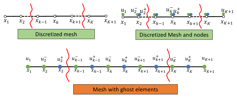
Figure 1: The Figure on top left shows the discretized mesh for a 1-dimensional domain. The top right figure shows the nodal unknowns for the discontinuous Galerkin based discretization approach. The bottom figure shows the physical mesh augmented with ghost elements. This allows the framework to predict discontinuous solutions.

4 Methodology

In this section, we develop the setting of the discontinuous Galerkin based deep learning framework proposed in this work. Taking motivation from the traditional finite element method (FEM) that solves for solution values at points (nodes) in the discretized domain, the framework is similarly used to predict nodal values. The nodal values are then interpolated by using piecewise continuous basis functions to yield a globally defined solution field. This approach allows us to construct a function of certain regularity (continuity and differentiability) in the whole domain, as opposed to obtaining a compositional function of certain differentiability, making the proposed approach uniquely advantageous. The polynomial order and the continuity of the interpolating basis functions can be further leveraged to generate nonlinear solutions with desired continuity requirements.

Figure 1 (top left) shows a discretized mesh in one dimension in which each element shares the nodes with a neighbouring element. Discontinuous Galerkin based technique adds additional degrees of freedom at each shared node along the faces of the elements as shown in Fig.1 (top right). In a similar spirit, we augment the physical mesh with ghost elements to allow the neural network to model jump or discontinuities in solutions as shown in Fig.1 (bottom).

Once the domain is discretized, we leverage the weak form of the governing equations to reduce the regularity requirements on the solution. The weak form is compared against the predefined basis functions from the test function space to obtain the physics-based loss (objective function). The integration is performed using Gauss quadrature schemes and the convolution operations are used to numerically evaluate the integrals in the weak form.

We note a few similarities and several differences with a previous research [37] that developed an FEM based neural architecture to solve PDEs (with continuous solutions). The approach presented therein relies on the use of an energy functional that can be minimized to yield the solution (Rayleigh-Ritz approach). However, the current work focuses on integrating discontinuous Galerkin based approach in a deep-learning based framework and relies on the minimization of the residual of the weak form.

4.1 Input and output for the framework

The input to the framework consists of the value of the solution field $\bm{u}^{t}$ at any time $t$. Based on the second order two stage Strong Stability Preserving Range-Kutta (SSP-RK) scheme [35, 36], the solution at the next time instant $\bm{u}^{t+\Delta t}$ is given as

$$\begin{split}&\bm{v}^{1}=\bm{u}^{t}+\Delta t\,\bm{\mathcal{NN}}(\bm{u}^{t};\theta),\\ \bm{u}^{t+\Delta t}&=\bm{u}^{t}+\frac{\Delta t}{2}\,\left(\bm{\mathcal{NN}}(\bm{u}^{t};\theta)+\bm{\mathcal{NN}}(\bm{v}^{1};\theta)\right),\end{split}$$ (7)

where $\bm{\mathcal{NN}}(\cdot;\theta)$ denotes the framework outputs. The solution field $\bm{u}^{t+\Delta t}$ becomes the input to the framework at time instant $t+\Delta t$. $\theta$ denotes the set of weights and biases of the network.

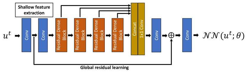
Figure 2: The Figure shows the architecture of the proposed framework.

4.2 Architecture

In this work, we implement the framework as a variant of the Residual Dense Network (RDN) originally proposed in [38]. In the context of PINNS, RDN has previously been shown to be successful in enhancing the spatial and temporal resolutions of coarse-scale (both in space and time) PDE solutions without requiring any labeled data [39, 40, 15]. Figure 2 shows the architecture of the proposed framework. The architecture consists of

1. Shallow feature extraction: Two convolutional layers are used to extract shallow features from the input state variable $u_{i}$ $(i=0,1,...,T-1)$, where $T$ denotes the total number of time steps. The output from the first convolutional layer is later reused below in step $4$.

2. Global feature fusion: Residual dense blocks with ReLU activation functions are then stacked together for extracting local dense features. The features extracted from all residual blocks are then concatenated together to exploit hierarchical features in a global way.

3. The concatenated hierarchical features are fed to a $1\times 1$ convolution layer to adaptively fuse a range of features with different levels followed by another convolution layer to further extract features for global residual learning.

4. Global residual learning: The shallow features (from step $1$) and the globally fused features (output from step $3$) are added together before the final output layer.

5. In the end, another convolutional layer is added to produce the output with desired dimensions.

4.3 Objective function

The solution to the system of equations (1) is obtained by solving the weak form (6) such that the norm of the residual $||\bm{\mathcal{R}}||$ becomes smaller than an acceptable tolerance value. In other words, the solution can also be written as the minimizer of the norm of residual $||\bm{\mathcal{R}}||$ such that $\bm{u}_{h}=\arg\min_{\bm{u}_{h}\in V_{h}}||\bm{\mathcal{R}}(\bm{u}_{h})||$. Therefore, the physics-informed objective function to be minimized during the training is given as follows:

$$\bm{u}_{h}(\theta)=\arg\min_{\theta}||\bm{\mathcal{R}}(\bm{u}_{h}(\theta))||_{1},$$ (8)

where $||\bm{A}||_{1}$ denotes the $L_{1}$ loss which is the mean absolute error (MAE) between each element in the quantity $\bm{A}$ and target $0$.

4.4 Boundary conditions

The proposed approach naturally accounts for the boundary conditions (Dirichlet and Neumann) without the need to treat them as extra penalty terms in the composite loss thereby avoiding issues arising during multi-objective optimization [41].

Dirichlet boundary conditions: Similar to finite element method based approaches, the Dirichlet boundary conditions are satisfied exactly in the framework. Once the framework predicts the solution at the next time step $\bm{u}^{t+\Delta t}$, a simple post-processing step is applied to append the known boundary values to the prediction. This process allows for exact imposition of Dirichlet boundary conditions without any additional penalty terms in the loss function. This process also eliminates the need to use distance functions (analytical or pre-trained models) to impose Dirichlet boundary conditions making the training process more interpretable.

Neumann boundary conditions: The natural boundary conditions are included in the weak form of the PDE. Therefore, the natural boundary conditions are automatically satisfied in the weak sense at the discrete form akin to its treatment in finite element based techniques.

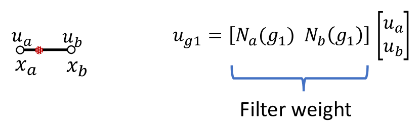
Figure 3: Figure showing a physical element from the mesh in $1$-$d$ and a gauss point $g_{1}$ marked in red. $x_{a}$ and $x_{b}$ denote the nodal coordinates. $u_{a}$ and $u_{b}$ denote the value of the solution at those nodal points. The equation on the right shows the convolution filter weight used to evaluate the value of the solution $u$ at the Gauss point $g_{1}$ (assuming linear interpolation). The filter weight can be obtained similarly when using higher order interpolation.

4.5 Integration and derivatives

Integration over the domain and boundaries in the finite element based approaches are simply calculated by evaluating the sum of the integration over individual elements interiors or elements boundaries

$$\begin{split}\int_{\Omega}fdV=\sum_{i=1}^{K}\int_{D^{k}}fdV\\ \int_{\partial\Omega}gdA=\sum_{i=1}^{K}\int_{\partial\mathcal{D}_{o}^{k}}gdA.\end{split}$$ (9)

where $D_{o}^{k}$ represents the exterior boundary for any element $D^{k}$. To numerically approximate the integrals, we use the Gaussian quadrature rule which is the weighted sum of integrand values at specified points within the domain of integration. We note that this evaluation of the integrand values inside the elements can be done with the use of a convolution operation. Figure 3 presents the visualization of the process of using a convolution operation for evaluating the integrand values at an interior point. For each quadrature point, the convolution filter is essentially the values of the interpolating basis functions at that point assembled together in a matrix (array in one dimension).

4.6 Training

The framework is implemented and trained using PyTorch. We use Adam optimizer with an initial learning rate of $1\times 10^{-3}$. As the training progresses, the learning rate is adjusted using ReduceLROnPlateau scheduler.

5 Results and discussion

For all the numerical experiments, the physical domain is distributed into $128$ equally spaced elements along the $x$-direction and $\Delta t=0.004$ is used. The architecture of the framework uses $4$ residual dense blocks with $8$ layers in each block. The growth rate and the number of features are set to $32$ in the model architecture. We use the same architecture for all the experiments and do not excessively tune hyperparameters individually for each case. The experiments are performed on an NVIDIA Tesla V100 GPU card with 32 GB RAM. For ease of presentation, we restrict the remainder of the section to a $1$-d spatial domain with a Cartesian mesh, although the framework is easily generalizable to polyhedral meshes. We also use linear shape functions in each (physical) element and a 2-point Gauss quadrature scheme to evaluate the integrals in the weak form.

5.1 Approximation of nonlinear function with a static discontinuity

In this test, we use the framework to solve a differential equation with static discontinuity at $x=0$ (i.e., the discontinuity stays fixed at $x=0$). The differential equation and the initial conditions are given as

$$\dot{u}(x,t)=\begin{cases}\cos(12x)&\quad x\geq 0\\ \sin(6x)&\quad x<0,\end{cases}$$

$$u(x,t=0)=\begin{cases}0.5\cos(12x)&\quad x\geq 0\\ 0.2\sin(6x)&\quad x<0.\end{cases}$$

The analytical solution is given as

$$u(x,t)=\begin{cases}(0.5+t)\cos(12x)&\quad x\geq 0\\ (0.2+t)\sin(6x)&\quad x<0.\end{cases}$$

Here, the domain is [-2, 2]. Figure 4 shows the solution obtained by the framework along with the analytical solution at three different time instants. We note that the obtained solution matches well with the analytical solution and successfully captures the discontinuity at $x=0$. As reflected from the Figure, the framework is also able to capture the high frequencies in the solution within $1000$ training epochs. The mean squared errors for the solutions presented in Fig. 4 are $\approx 2\times 10^{-10}$. Therefore, we conclude that the framework successfully captures the discontinuity at $x=0$ with high accuracy without the need for any adaptive refinement or a-priori knowledge of the location of the discontinuity.

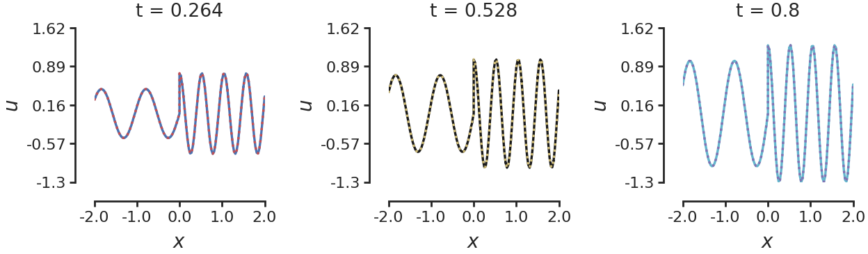
Figure 4: The figure shows the solution of an ordinary differential equation with static discontinuity (jump at $x=0$) at three different time instants. Solid lines represents the solution obtained from the framework and dashed lines represents the exact solution.

5.2 Advection equation

In this section, we consider a one-dimensional advection equation that has the following mathematical form

$$\frac{\partial u(x,t)}{\partial t}+v(x,t)\frac{\partial u(x,t)}{\partial x}=0.$$ (10)

We present the results for the following two cases: a) Smooth initial condition and b) Discontinuous initial condition. For both the cases, we take the domain $x\in[-2,2]$ and the velocity field to be constant, i.e. $v(x,t)=1$. We note that the traditional finite element method fails to converge when solving the advection equation. Therefore, a discontinuous Galerkin based discretization is an obvious choice.

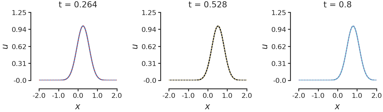
Figure 5: The figure shows the solution of the advection equation with smooth initial condition at three different time instants. Solid lines represents the solution obtained from the framework and dashed lines represents the exact solution.

5.2.1 Smooth initial condition

This section focuses on applying the framework to solve the advection equation with continuous initial conditions given by

$$u(x,t=0) =e^{-5x^{2}},~{}~{}~{}~{}\forall~{}x\in[-2,2].$$ (11)

The boundary condition at $x=-2$ is taken as $u(x=-2,t)=0$. The analytical solution for this problem is the traveling wave solution $u(x,t)=e^{-5(x-t)^{2}}$. Figure 5 shows the results obtained from the framework along with the analytical solution at three different time instants. The framework is able to solve the advection equation with great accuracy and is able to match the analytical travelling wave solution. This verifies our implementation of the discontinuous Galerkin discretization within the convolutional neural network framework.

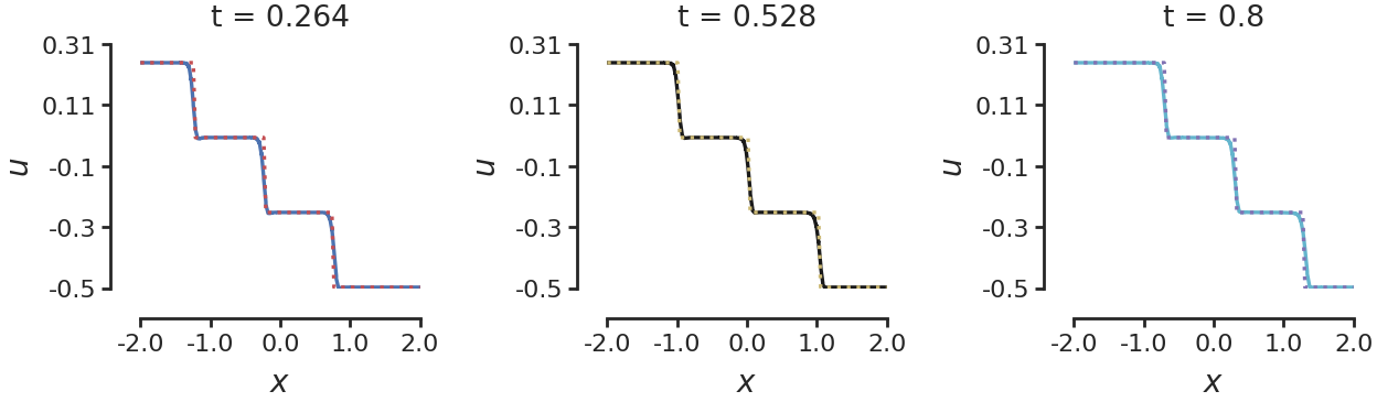
Figure 6: The figure shows the solution of the advection equation with jumps in the initial condition at three different time instants. Solid lines represents the solution obtained from the framework and dashed lines represents the exact solution.

5.2.2 Discontinuous initial condition

This section focuses on applying the framework to solve the advection equation with discontinuous initial conditions. The initial and boundary conditions are given as

$$u(x,t=0) =\begin{cases}0.25&\quad x\leq-1.5\\ 0.0&\quad x>-1.5~{}\text{and}~{}x\leq-0.5\\ -0.25&\quad x>-0.5~{}\text{and}~{}x\leq 0.5\\ -0.5&\quad\text{otherwise}.\end{cases},~{}~{}~{}~{}\forall~{}x\in[-2,2]$$ (12)

$$u(x=-2,t) =0.25.$$ (13)

The analytical solution for this problem is the traveling wave solution given by

$$u(x,t) =\begin{cases}0.25&\quad x-t\leq-1.5\\ 0.0&\quad x-t>-1.5~{}\text{and}~{}x-t\leq-0.5\\ -0.25&\quad x-t>-0.5~{}\text{and}~{}x-t\leq 0.5\\ -0.5&\quad\text{otherwise}.\end{cases},~{}~{}~{}~{}\forall~{}x\in[-2,2]$$ (14)

We note that the location of the discontinuity (jump in solution) moves in space as the time progresses. For the conventional PINN based approaches, solving the advection equation with such an initial condition would necessitate the use of residual based adaptive refinement. The approach would also require a large amount of training data in the regions of sharp gradients. However, in the absence of any labeled data, such an information is usually not known a-priori. Therefore, traditional PINN based approaches face serious difficulties in capturing the sharp gradients in the solutions.

Figure 6 shows the comparison of the solution obtained from the framework with the analytical solution at three different time instants. The framework is able to resolve the sharp jumps in solution at all times without any apriori knowledge of its location or use of adaptive refinement.

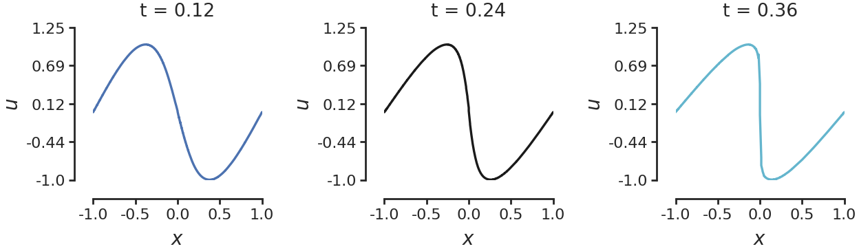
Figure 7: The figure shows the solution of the inviscid Burgers equation with periodic boundaries and sinusoidal initial condition at three different time instants. Solid lines represents the solution obtained from the framework and dashed lines represents the exact solution.

Comparison with other works
Collocation points	Reference	Disadvantage
300	[27]	• Requires computationally expensive fifth-order WENO finite difference scheme [42, see Table 6] • Not amenable to unstructured grids
10,000	[28]	• Requires Large number of collocation points • Effectiveness of the weight is yet to be demonstrated for general problems
4,141	[22]	• Breaks the domain into smaller smaller sub domains requires location of the discontinuity to be known a-priori
–	[24, 25, 28, 22, 29, 19, 23]	Solve viscous Burgers equation

Table 1: Table mentioning the other works that solve the inviscid Burgers equation and its disadvantages as compared with the proposed framework.

5.3 Burgers equation

We apply our discontinuous Galerkin based deep-learning framework to solve an inviscid Burgers equation in this section. The inviscid Burgers equation is a nonlinear first order hyperbolic PDE that can develop shocks or discontinuities even if the initial data is smooth. Therefore, it has become a standard benchmark to demonstrate the shock capturing ability of any numerical scheme including PINN based approaches. The one dimensional inviscid Burgers equation is given as

$$\frac{\partial u(x,t)}{\partial t}+u(x,t)\frac{\partial u(x,t)}{\partial x}=0,~{}~{}~{}~{}~{}~{}\forall~{}x\in[-1,1].$$ (15)

We use a sinusoidal initial condition with periodic boundaries in this work, i.e.

$$u(x,t=0)=-\sin(\pi x)$$ (16)

$$u(x=-1,t)=u(x=1,t)=0.$$ (17)

The exact solution to the Burgers equation for these set of initial and boundary conditions develops a shock at $x=0$. Table 1 presents brief details of some of the other works that solve inviscid Burgers equation using physics informed neural networks.

Figure 7 shows the solution obtained from the framework at three different time instants. We notice that the framework is able to solve the Burgers equation with great accuracy without any need for adaptive refinement or a-priori knowledge of the location of the discontinuity. The framework is successfully able to approximate the solution to the inviscid Burgers equation which involves self steepening into a sharp profile at $x=0$ even when the initial condition is a smooth sinusoidal wave.

6 Conclusion

This research focused on the development of deep-learning based framework that can predict discontinuous solutions to nonlinear PDEs without any a-priori knowledge of the solution or the location of the discontinuities. The work takes motivation from the traditional discontinuous Galerkin based finite element method (FEM) that solves for solution values at points (nodes) in the discretized domain. These nodal values are interpolated by using piecewise continuous basis functions to yield a globally defined solution field. The polynomial order and the continuity of the interpolating basis functions is leveraged to generate nonlinear solutions with desired continuity requirements. The physical mesh is augmented with ghost elements to allow for jump in solutions and integration is performed using Gauss point quadrature schemes. Built on the rigorous mathematical foundations of the discontinuous Galerkin method, the framework naturally handles imposition of boundary conditions (Neumann/Dirichlet), entropy conditions, and regularity requirements. Several numerical experiments and validation with analytical solutions demonstrate the accuracy, robustness, and effectiveness of the proposed framework.

The current work also paves the way for the following extensions in the future works:

• Given the generality and universality of the proposed formalism, the framework can be easily extended to multi-dimensions and applied to study a wide range of problems in fluid in solid mechanics. Furthermore, studying the effects of high-order piecewise polynomials and slope-limiters on model accuracy and convergence is another interesting research area to pursue.

• The future research will also study the h-convergence (mesh convergence) and p-convergence (convergence based on basis order) of the framework analogous to the convergence analysis of the finite element based solution to PDEs.

• Although the current work focuses on the forward problems, future work would also focus on applying the framework to study inverse problems and parametric PDEs where PDEs are defined by a family of parametrized physical properties or boundary conditions.

• The future works of this research will focus on presenting a more comprehensive evaluation of framework’s performance against other PINN based approaches while studying nonlinear problems with moving shocks/discontinuities in higher dimensions.

• The extension of the framework to arbitrary triangulations can be done via coordinate transformation between the physical and reference domains [43]. However, the use of Graph Neural Networks (GNN) to account for the mesh structural information and learning over unstructured grids and complex topological structures is another interesting avenue to pursue.

• The use of Local Discontinuous Galerkin (LDG) method to solve equations with higher order derivatives is a work in progress.

References

- [1] John David Anderson and John Wendt. Computational fluid dynamics, volume 206. Springer, 1995.
- [2] Javier Bonet, Antonio J Gil, Chun Hean Lee, Miquel Aguirre, and Rogelio Ortigosa. A first order hyperbolic framework for large strain computational solid dynamics. part i: Total lagrangian isothermal elasticity. Computer Methods in Applied Mechanics and Engineering, 283:689–732, 2015.
- [3] Jan Achenbach. Wave propagation in elastic solids. Elsevier, 2012.
- [4] Rajat Arora. Computational Approximation of Mesoscale Field Dislocation Mechanics at Finite Deformation. PhD thesis, Carnegie Mellon University, 2019.
- [5] Rinaldo M Colombo. Hyperbolic phase transitions in traffic flow. SIAM Journal on Applied Mathematics, 63(2):708–721, 2003.
- [6] Christopher KW Tam and Jay C Webb. Dispersion-relation-preserving finite difference schemes for computational acoustics. Journal of computational physics, 107(2):262–281, 1993.
- [7] J Blake Temple. Solutions in the large for the nonlinear hyperbolic conservation laws of gas dynamics. Journal of Differential Equations, 41(1):96–161, 1981.
- [8] Constantine M Dafermos and Constantine M Dafermos. Hyperbolic conservation laws in continuum physics, volume 3. Springer, 2005.
- [9] Bernardo Cockburn, George E Karniadakis, and Chi-Wang Shu. Discontinuous Galerkin methods: theory, computation and applications, volume 11. Springer Science & Business Media, 2012.
- [10] Gary A Sod. A survey of several finite difference methods for systems of nonlinear hyperbolic conservation laws. Journal of computational physics, 27(1):1–31, 1978.
- [11] Randall J LeVeque et al. Finite volume methods for hyperbolic problems, volume 31. Cambridge university press, 2002.
- [12] Stanley Osher and Fred Solomon. Upwind difference schemes for hyperbolic systems of conservation laws. Mathematics of computation, 38(158):339–374, 1982.
- [13] Peter K Sweby. High resolution schemes using flux limiters for hyperbolic conservation laws. SIAM journal on numerical analysis, 21(5):995–1011, 1984.
- [14] Rajat Arora, Pratik Kakkar, Biswadip Dey, and Amit Chakraborty. Physics-informed neural networks for modeling rate-and temperature-dependent plasticity. arXiv preprint arXiv:2201.08363, 2022.
- [15] Rajat Arora and Ankit Shrivastava. Spatio-temporal super-resolution of dynamical systems using physics-informed deep-learning. arXiv preprint arXiv:2212.04457, 2022.
- [16] Ameya D Jagtap, Zhiping Mao, Nikolaus Adams, and George Em Karniadakis. Physics-informed neural networks for inverse problems in supersonic flows. arXiv preprint arXiv:2202.11821, 2022.
- [17] Olga Fuks and Hamdi A Tchelepi. Limitations of physics informed machine learning for nonlinear two-phase transport in porous media. Journal of Machine Learning for Modeling and Computing, 1(1), 2020.
- [18] Siddhartha Mishra and Roberto Molinaro. Estimates on the generalization error of physics-informed neural networks for approximating a class of inverse problems for pdes. IMA Journal of Numerical Analysis, 42(2):981–1022, 2022.
- [19] Ravi G Patel, Indu Manickam, Nathaniel A Trask, Mitchell A Wood, Myoungkyu Lee, Ignacio Tomas, and Eric C Cyr. Thermodynamically consistent physics-informed neural networks for hyperbolic systems. Journal of Computational Physics, 449:110754, 2022.
- [20] Zhiping Mao, Ameya D Jagtap, and George Em Karniadakis. Physics-informed neural networks for high-speed flows. Computer Methods in Applied Mechanics and Engineering, 360:112789, 2020.
- [21] Ameya D Jagtap and George E Karniadakis. Extended physics-informed neural networks (xpinns): A generalized space-time domain decomposition based deep learning framework for nonlinear partial differential equations. In AAAI Spring Symposium: MLPS, 2021.
- [22] Vikas Dwivedi, Nishant Parashar, and Balaji Srinivasan. Distributed physics informed neural network for data-efficient solution to partial differential equations. arXiv preprint arXiv:1907.08967, 2019.
- [23] Ameya D Jagtap, Ehsan Kharazmi, and George Em Karniadakis. Conservative physics-informed neural networks on discrete domains for conservation laws: Applications to forward and inverse problems. Computer Methods in Applied Mechanics and Engineering, 365:113028, 2020.
- [24] Maziar Raissi, Paris Perdikaris, and George Em Karniadakis. Physics informed deep learning (part i): Data-driven solutions of nonlinear partial differential equations. arXiv preprint arXiv:1711.10561, 2017.
- [25] Ameya D Jagtap, Kenji Kawaguchi, and George Em Karniadakis. Adaptive activation functions accelerate convergence in deep and physics-informed neural networks. Journal of Computational Physics, 404:109136, 2020.
- [26] Lu Lu, Xuhui Meng, Zhiping Mao, and George Em Karniadakis. Deepxde: A deep learning library for solving differential equations. SIAM Review, 63(1):208–228, 2021.
- [27] Chunyue Lv, Lei Wang, and Chenming Xie. A hybrid physics-informed neural network for nonlinear partial differential equation. arXiv preprint arXiv:2112.01696, 2021.
- [28] Li Liu, Shengping Liu, Heng Yong, Fansheng Xiong, and Tengchao Yu. Discontinuity computing with physics-informed neural network. arXiv preprint arXiv:2206.03864, 2022.
- [29] Emilio Jose Rocha Coutinho, Marcelo Dall’Aqua, Levi McClenny, Ming Zhong, Ulisses Braga-Neto, and Eduardo Gildin. Physics-informed neural networks with adaptive localized artificial viscosity. arXiv preprint arXiv:2203.08802, 2022.
- [30] Tim De Ryck, Siddhartha Mishra, and Roberto Molinaro. wpinns: Weak physics informed neural networks for approximating entropy solutions of hyperbolic conservation laws. arXiv preprint arXiv:2207.08483, 2022.
- [31] Ruben Rodriguez-Torrado, Pablo Ruiz, Luis Cueto-Felgueroso, Michael Cerny Green, Tyler Friesen, Sebastien Matringe, and Julian Togelius. Physics-informed attention-based neural network for hyperbolic partial differential equations: application to the buckley–leverett problem. Scientific reports, 12(1):1–12, 2022.
- [32] Shiying Xiong, Xingzhe He, Yunjin Tong, Runze Liu, and Bo Zhu. RoeNets: predicting discontinuity of hyperbolic systems from continuous data. arXiv preprint arXiv:2006.04180, 2020.
- [33] Jingrun Chen, Shi Jin, and Liyao Lyu. A deep learning based discontinuous galerkin method for hyperbolic equations with discontinuous solutions and random uncertainties. arXiv preprint arXiv:2107.01127, 2021.
- [34] William H Reed and Thomas R Hill. Triangular mesh methods for the neutron transport equation. Technical report, Los Alamos Scientific Lab., N. Mex.(USA), 1973.
- [35] Sigal Gottlieb and Chi-Wang Shu. Total variation diminishing runge-kutta schemes. Mathematics of computation, 67(221):73–85, 1998.
- [36] Sigal Gottlieb, Chi-Wang Shu, and Eitan Tadmor. Strong stability-preserving high-order time discretization methods. SIAM review, 43(1):89–112, 2001.
- [37] Biswajit Khara, Aditya Balu, Ameya Joshi, Soumik Sarkar, Chinmay Hegde, Adarsh Krishnamurthy, and Baskar Ganapathysubramanian. Neufenet: Neural finite element solutions with theoretical bounds for parametric pdes. arXiv preprint arXiv:2110.01601, 2021.
- [38] Yulun Zhang, Yapeng Tian, Yu Kong, Bineng Zhong, and Yun Fu. Residual dense network for image super-resolution. In Proceedings of the IEEE conference on computer vision and pattern recognition, pages 2472–2481, 2018.
- [39] Rajat Arora. Machine learning-accelerated computational solid mechanics: Application to linear elasticity. arXiv preprint arXiv:2112.08676, 2021.
- [40] Rajat Arora. PhySRNet: Physics informed super-resolution network for application in computational solid mechanics. arXiv preprint arXiv:2206.15457, 2022.
- [41] Sifan Wang, Yujun Teng, and Paris Perdikaris. Understanding and mitigating gradient pathologies in physics-informed neural networks. arXiv preprint arXiv:2001.04536, 2020.
- [42] Rafael Borges, Monique Carmona, Bruno Costa, and Wai Sun Don. An improved weighted essentially non-oscillatory scheme for hyperbolic conservation laws. Journal of Computational Physics, 227(6):3191–3211, 2008.
- [43] Han Gao, Luning Sun, and Jian-Xun Wang. Phygeonet: Physics-informed geometry-adaptive convolutional neural networks for solving parametric pdes on irregular domain. arXiv e-prints, pages arXiv–2004, 2020.
- [44] Rajat Arora and Amit Acharya. Dislocation pattern formation in finite deformation crystal plasticity. International Journal of Solids and Structures, 184:114–135, 2020.
- [45] Rajat Arora and Amit Acharya. A unification of finite deformation J2 Von-Mises plasticity and quantitative dislocation mechanics. Journal of the Mechanics and Physics of Solids, 143:104050, 2020.
- [46] Rajat Arora, Xiaohan Zhang, and Amit Acharya. Finite element approximation of finite deformation dislocation mechanics. Computer Methods in Applied Mechanics and Engineering, 367:113076, 2020.
- [47] Abhishek Arora, Rajat Arora, and Amit Acharya. Mechanics of micropillar confined thin film plasticity. arXiv preprint arXiv:2202.06410, 2022.
- [48] Tushar Joshi, Rajat Arora, Anup Basak, and Anurag Gupta. Equilibrium shape of misfitting precipitates with anisotropic elasticity and anisotropic interfacial energy. Modelling and Simulation in Materials Science and Engineering, 28(7):075009, 2020.
- [49] Rajat Arora, Sukhdeep Singh Sandhu, and Paridhi Agarwal. A proposal for deployment of wireless sensor network in day-to-day home and industrial appliances for a greener environment. In Proceedings of the Second International Conference on Soft Computing for Problem Solving (SocProS 2012), December 28-30, 2012, pages 1081–1086. Springer, 2014.