Model-Based End-to-End Learning for Multi-Target Integrated Sensing and Communication

Abstract

We study model-based end-to-end learning in the context of integrated sensing and communication (ISAC) under hardware impairments. A monostatic orthogonal frequency-division multiplexing (OFDM) sensing and multiple-input single-output (MISO) communication scenario is considered, incorporating hardware imperfections at the ISAC transceiver antenna array. To enable end-to-end learning of the ISAC transmitter and sensing receiver, we propose a novel differentiable version of the orthogonal matching pursuit (OMP) algorithm that is suitable for multi-target sensing. Based on the differentiable OMP, we devise two model-based parameterization strategies to account for hardware impairments: (i) learning a dictionary of steering vectors for different angles, and (ii) learning the parameterized hardware impairments. For the single-target case, we carry out a comprehensive performance analysis of the proposed model-based learning approaches, a neural-network-based learning approach and a strong baseline consisting of least-squares beamforming, conventional OMP, and maximum-likelihood symbol detection for communication. Results show that learning the parameterized hardware impairments offers higher detection probability, better angle and range estimation accuracy, lower communication symbol error rate (SER), and exhibits the lowest complexity among all learning methods. Lastly, we demonstrate that learning the parameterized hardware impairments is scalable also to multiple targets, revealing significant improvements in terms of ISAC performance over the baseline.

I Introduction

Next-generation wireless communication systems are expected to operate at higher carrier frequencies to meet the data rate requirements necessary for emerging use cases such as smart cities, e-health, and digital twins for manufacturing [1, 2, 3, 4]. Higher carrier frequencies also enable new functionalities, such as integrated sensing and communication (ISAC). ISAC aims to integrate radar and communication capabilities in one joint system, which enables hardware sharing, energy savings, communication in high-frequency radar bands, and improved channel estimation via sensing-assisted communications, among other advantages [5, 6, 7, 8, 9]. ISAC has been mainly considered by means of dual-functional waveforms. For instance, radar signals have been used for communication [10, 11], while communication waveforms have proven to yield radar-like capabilities [8, 12]. Furthermore, optimization of waveforms to perform both tasks simultaneously has also been studied [5, 13, 14, 15, 16, 17, 18], where the results depend on the cost function to optimize and the ISAC optimization variables. However, conventional ISAC approaches degrade in performance under model mismatch, i.e., if the underlying reality does not match the assumed mathematical models. In particular at high carrier frequencies, hardware impairments can severely affect the system performance and hardware design becomes very challenging [19, 20]. This increases the likelihood of model mismatch in standard approaches, and problems become increasingly difficult to solve analytically if hardware impairments are considered.

DL approaches based on large neural networks have proven to be useful under model mismatch or complex optimization problems [21, 22]. DL does not require any knowledge about the underlying models as it is optimized based on training data, which inherently captures the potential impairments of the system. DL has been investigated in the context of ISAC for a vast range of applications, such as predictive beamforming in vehicular networks [23, 24, 25], waveform design [26] and channel estimation [27] in intelligent reflecting surface (IRS)-assisted ISAC scenarios, multi-target sensing and communication in THz transmissions [28], or efficient resource management [29, 30]. However, most previous works on DL for ISAC consider single-component optimization, either at the transmitter or receiver. On the other hand, end-to-end learning [31] of both the transmitter and receiver has proven to enhance the final performance of radar [32] and communication [33] systems. End-to-end learning in ISAC was applied by means of an autoencoder (AE) architecture in [34], to perform single-target angle estimation and communication symbol estimation, under hardware impairments. This was recently extended to multiple targets in [35], although without considering impairments, where the AE outperformed conventional ESPRIT [36] in terms of angle estimation for single- and dual-snapshot transmissions. Nevertheless, deep learning (DL) approaches often lack interpretability and require large amounts of training data to obtain satisfactory performance.

To overcome the disadvantages of large DL models, model-based machine learning (MB-ML) [37] instead parameterizes existing models and algorithms while maintaining their overall computation graph as a blueprint. This allows training initialization from an already good starting point, requiring less training data to optimize, and typically also offers a better understanding of the learned parameters. A popular example of MB-ML learning is deep unfolding [38, 39, 40], where iterative algorithms are “unrolled” and interpreted as multi-layer computation graphs. In the context of sensing, deep unfolding of the fixed-point continuation algorithm with one-sided $l_{1}$-norm was applied to angle estimation of multiple targets [41], showing enhanced accuracy with respect to DL and model-based benchmark approaches. In [42], the iterative shrinkage-thresholding algorithm (ISTA) was unfolded to perform angle estimation in the presence of array imperfections. Related to communications, deep unfolding has been applied to massive multiple-input multiple-output (MIMO) channel estimation in [43], where classical steering vector models are used as a starting point and then optimized to learn the system hardware impairments, by unfolding the matching pursuit algorithm [44]. This approach was later refined to reduce the required number of learnable parameters in [45]. Previous MB-ML approaches [41, 42, 43, 45] exhibit three primary shortcomings that can limit their effectiveness in practical scenarios. Firstly, they focus only on receiver learning; however, end-to-end learning of transmitter and receiver, which holds great potential given its promising performance in model-free DL applications [32, 33], remains unexplored in MB-ML. Secondly, sensing works [41, 42] only investigate angle estimation, although range estimation is also required to estimate target locations. Hence, end-to-end MB-ML for multi-target positioning has not been studied before. Finally, while MB-ML has been utilized to address individual challenges related to sensing and communications, its untapped potential to significantly improve system performance in ISAC applications remains undiscovered.

In view of the current literature on DL and MB-ML for ISAC, three questions arise: (i) How can efficient end-to-end MB-ML strategies be developed for multi-target positioning? (ii) What computational and performance benefits can be harnessed by employing MB-ML in ISAC systems compared to large DL models and model-based approaches? (iii) To what extent can ISAC trade-offs be improved under hardware impairments by employing MB-ML strategies compared to large DL models and model-based approaches?

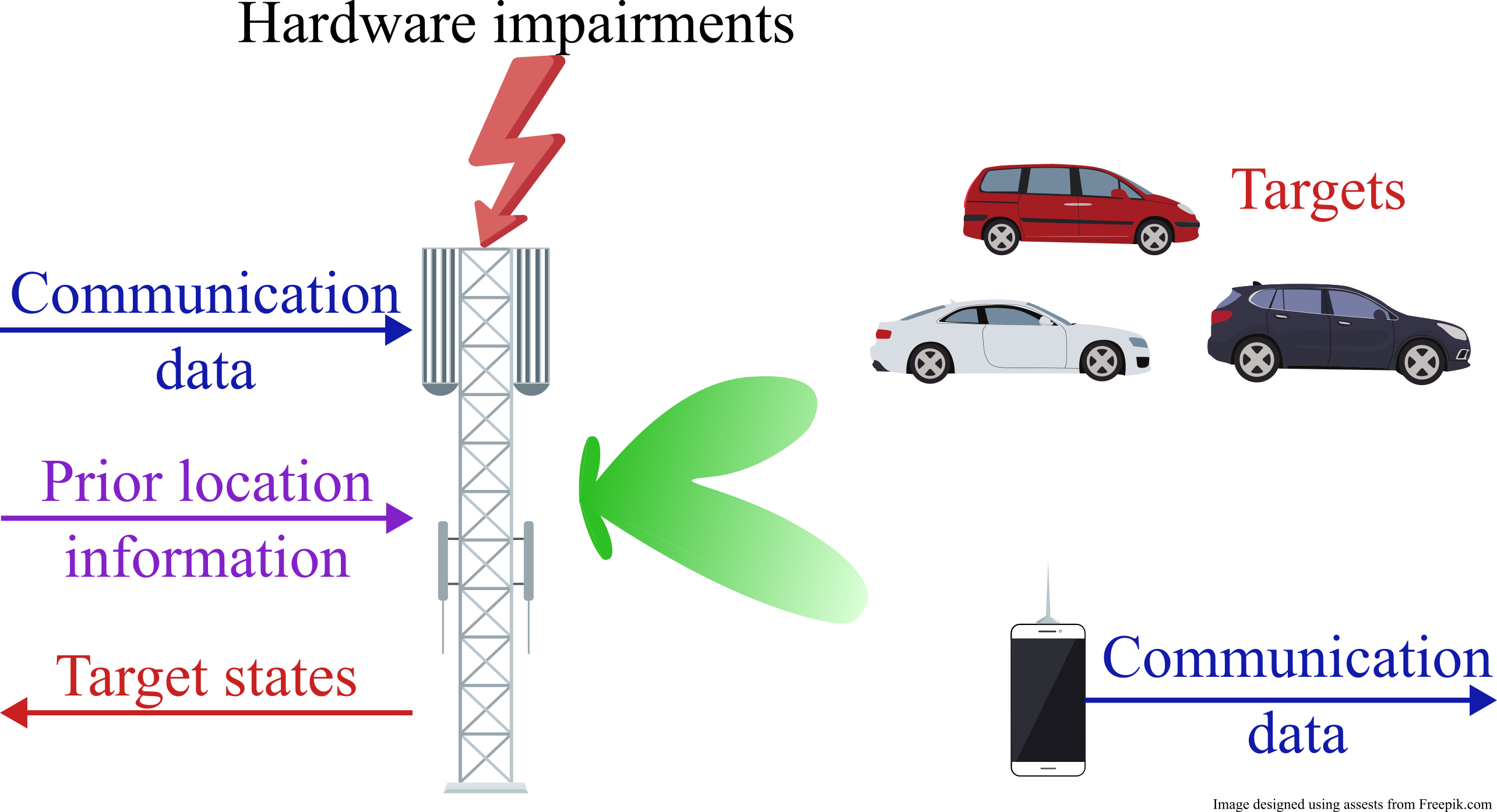
Figure 1: Considered scenario, where an impaired multi-antenna ISAC transmitter is optimized based on prior information of the location of the targets and the communication receiver. The co-located sensing receiver estimates the targets’ states (target probability and position), while the single-antenna communication receiver retrieves the transmitted communication data.

This paper aims to answer the above questions by studying end-to-end MB-ML for ISAC, focusing on the effect of hardware impairments in the ISAC transceiver uniform linear array (ULA). Considering a MIMO monostatic sensing and multiple-input single-output (MISO) communication scenario (as depicted in Fig. 1), we propose novel end-to-end MB-ML strategies for joint optimization of the ISAC transmitter and sensing receiver, suitable for both single- and multi-target scenarios. Building upon our preliminary analysis in [46], the main contributions of this work can be summarized as follows:

• Multi-target position estimation via end-to-end learning of orthogonal frequency-division multiplexing (OFDM) ISAC systems: For the first time in the literature, we investigate end-to-end learning of OFDM ISAC systems under hardware impairments at the ISAC ULA. To combat these hardware imperfections, we introduce novel learning architectures to simultaneously optimize the ISAC beamformer and sensing receiver. OFDM transmission enables joint angle and range (and, hence, position) estimation of multiple targets, significantly extending the single-carrier models and methods in our previous work [46], and the recent works [34, 35].

• MB-ML via differentiable orthogonal matching pursuit (OMP): Expanding upon the foundation laid by [43, 45], we propose a differentiable version of the OMP algorithm that is suitable for single- and multi-target sensing. This new algorithm allows for end-to-end gradient-based optimization, where we consider two different MB-ML parameterization approaches. The first approach learns a dictionary of steering vectors at each OMP iteration, extending our results in [46] to joint range-angle estimation and multiple targets. The second approach is new compared to [46] and directly learns the parameterized ULA impairments at each iteration. This offers the advantage of drastically reducing the number of parameters to be learned.

• Single- and multi-target performance comparison and ISAC trade-off characterization: We first consider the single-target case (corresponding to one OMP iteration) and compare different solutions based on the extent of model knowledge: (i) neural-network-based learning (NNBL), representing no knowledge of the system model, (ii) the two MB-ML approaches, where model knowledge is utilized, but impairments are learned, and (iii) a strong baseline, which fully relies on the mathematical description of the system model under no hardware impairments. Our results show that under hardware impairments, the new MB-ML ULA impairment learning outperforms all other approaches in terms of target detection and range-angle estimation, with fewer trainable parameters. Lastly, we show that impairment learning scales smoothly also to multiple targets, where it achieves better sensing and communication performance than the baseline.

In the rest of this paper, we first describe the mathematical ISAC system model in Sec. II. Then, we describe the two approaches to perform target positioning and communication: the baseline in Sec. III, and MB-ML in Sec. IV. The main ISAC results are presented and discussed in Sec. V before the concluding remarks of Sec. VI.

Notation. We denote column vectors as bold-faced lower-case letters, $\bm{a}$, and matrices as bold-faced upper-case letters, $\bm{A}$. A column vector whose entries are all equal to 1 is denoted as $\bm{1}$. The identity matrix of size $N\times N$ is denoted as $\bm{I}_{N}$. The transpose and conjugate transpose operations are denoted by $(\cdot)^{\top}$ and $(\cdot)^{\mathsf{H}}$, respectively. The $i$-th element of a vector and the $(i,j)$-th element of a matrix are denoted by $[\bm{a}]_{i}$ and $[\bm{A}]_{i,j}$. The element-wise product between two matrices is denoted by $\bm{A}\odot\bm{B}$, while $\oslash$ denotes element-wise division, and $\otimes$ denotes the Kronecker product. ${\rm{vec}}(\cdot)$ denotes matrix vectorization operator. Sets of elements are enclosed by curly brackets and intervals are enclosed by square brackets. The set $\{x\in\mathbb{R}|x\geq 0\}$ is denoted as $\mathbb{R}_{\geq 0}$. The cardinality of a set $\mathcal{X}$ is denoted by $\lvert\mathcal{X}\rvert$. The uniform distribution is denoted by $\mathcal{U}$, and $\mathcal{CN}$ denotes the circularly-symmetric complex distribution. The Euclidean vector norm is represented by $\lVert\cdot\rVert_{2}$, while the matrix Frobenius norm is denoted by $\lVert\cdot\rVert_{F}$. The indicator function is denoted by $\mathbb{I}\{\cdot\}$.

II System Model

[width=mode=buildnew]figures/system_model

Figure 2: Block diagram of the ISAC system model. The colored blocks can be implemented following standard neural-network-based learning [34, 35], the baseline of Secs. III-A, III-B, or model-based learning of Sec. IV. The precoding block applies the same mapping function for sensing and communication. Note that the sensing estimator is co-located with the ISAC transmitter.

This section provides the mathematical models for the received sensing and communication signals, the ISAC transmitted signal and the hardware impairments. In Fig. 2, a block diagram of the considered ISAC system is depicted.

II-A Multi-target MIMO Sensing

We consider an ISAC transceiver consisting of an ISAC transmitter and a sensing receiver sharing the same ULA of $K$ antennas, as shown in Fig. 1. The transmitted signal consists of an OFDM waveform across $S$ subcarriers, with an inter-carrier spacing of $\Delta_{f}$ Hz. In the sensing channel, we consider at most $T_{\rm{max}}$ possible targets. Then, the backscattered signal impinging onto the sensing receiver can be expressed over antenna elements and subcarriers as [47, 48, 49]

$$\bm{Y}_{r}=\frac{1}{\sqrt{S}}\sum_{t=1}^{T}\psi_{t}\bm{a}(\theta_{t})\bm{a}^{\top}(\theta_{t})\bm{f}[\bm{x}(\bm{m})\odot\bm{\rho}(\tau_{t})]^{\top}+\bm{W},$$ (1)

where $\bm{Y}_{r}\in\mathbb{C}^{K\times S}$ collects the observations in the spatial-frequency domains, $T\sim\mathcal{U}\{0,...,T_{\rm{max}}\}$ is the instantaneous number of targets in the scene, and $\psi_{t}\sim\mathcal{CN}(0,\sigma_{r}^{2})$ represents the complex channel gain of the $t$-th target. The steering vector of the ISAC transceiver ULA for an angular direction $\theta$ is, under no hardware impairments, $[\bm{a}(\theta)]_{k}=\exp(-\jmath 2\pi(k-(K-1)/2)d\sin(\theta)/\lambda)$, $k=0,...,K-1$, with $d=\lambda/2$, $\lambda=c/f_{c}$, $c$ is the speed of light in vacuum and $f_{c}$ is the carrier frequency. The precoder $\bm{f}\in\mathbb{C}^{K}$ permits to steer the antenna energy into a particular direction. Target ranges are conveyed by $\bm{\rho}(\tau_{t})\in\mathbb{C}^{S}$, with $[\bm{\rho}(\tau_{t})]_{s}=\exp(-j2\pi s\Delta_{f}\tau_{t})$, $s=0,...,S-1$, and where $\tau_{t}=2R_{t}/c$ represents the round-trip time of the $t$-th target at $R_{t}$ meters away from the transmitter. Moreover, the communication symbol vector $\bm{x}(\bm{m})\in\mathbb{C}^{S}$ conveys a vector of messages $\bm{m}\in\mathcal{M}^{S}$, each uniformly distributed from a set of possible messages $\mathcal{M}$. Finally, the receiver noise is represented by $\bm{W}$, with $[\bm{W}]_{i,j}\sim\mathcal{CN}(0,N_{0})$. Note that if $T=0$, only noise is received. From the complex channel gain and the noise, we define the integrated sensing signal-to-noise ratio (SNR) across antenna elements as $\text{SNR}_{r}=K\sigma_{r}^{2}/N_{0}$.

The angles and ranges of the targets are uniformly distributed within an uncertainty region, i.e., $\theta_{t}\sim\mathcal{U}[\theta_{\min},\theta_{\max}]$ and $R_{t}\sim\mathcal{U}[R_{\min},R_{\max}]$. However, uncertainty regions might change at each new transmission. The position of each target is computed from target angle $\theta_{t}$ and range $R_{t}$ as

$$\bm{p}_{t}=\begin{bmatrix}R_{t}\cos{(\theta_{t})}\\ R_{t}\sin{(\theta_{t})}\end{bmatrix}.$$ (2)

The transmitter and the sensing receiver are assumed to have knowledge of $\{\theta_{\min},\theta_{\max},R_{\min},R_{\max}\}$. In the considered monostatic sensing setup, the receiver has access to communication data $\bm{x}(\bm{m})$, which enables removing its impact on the received signal (1) via reciprocal filtering [50, 51]

$$\widetilde{\bm{Y}}_{r}=\bm{Y}_{r}\oslash{{\bm{1}}}\bm{x}^{\top}(\bm{m})=\sum_{t=1}^{T}\alpha_{t}\bm{a}(\theta_{t})\bm{\rho}^{\top}(\tau_{t})+\bm{N}~{},$$ (3)

where $\alpha_{t}=\frac{1}{\sqrt{S}}\bm{a}^{\top}(\theta_{t})\bm{f}\psi_{t}$ and $\bm{N}=\bm{W}\oslash{{\bm{1}}}\bm{x}^{\top}(\bm{m})$. The goal of the sensing receiver is to estimate the presence probability of each target in the scene, denoted as $\hat{\bm{u}}\in[0,1]^{T_{\rm{max}}}$, which is later thresholded to provide a hard estimate of the target presence, $\hat{\bm{t}}\in\{0,1\}^{T_{\rm{max}}}$. For all detected targets, the sensing receiver estimates their angles, $\hat{\bm{\theta}}\in[-\pi/2,\pi/2]^{T_{\rm{max}}}$, and their ranges, $\hat{\bm{R}}\in\mathbb{R}_{\geq 0}^{T_{\rm{max}}}$, from which target positions can be estimated according to (2).

II-B MISO Communication

In the considered ISAC scenario, communication and sensing share the same transmitter. We assume that the communication receiver is equipped with a single antenna element. In this setting, the received OFDM signal at the communication receiver in the frequency domain is given by [52]

$$\bm{y_{c}}=[\bm{x}(\bm{m})\odot\bm{\beta}]\bm{f}^{\top}\bm{a}(\varphi)+\bm{n},$$ (4)

with $\bm{\beta}\in\mathbb{C}^{S}$ denoting the $S$-point discrete Fourier transform (DFT) of the channel taps $[\beta_{0},\beta_{1},...,\beta_{L-1},0,...,0]$, where each tap is distributed as $\beta_{l}\sim\mathcal{CN}(0,\sigma_{l}^{2})$. Complex Gaussian noise $\bm{n}\sim\mathcal{CN}(\bm{0},N_{0}\bm{I}_{S})$ is added at the receiver side. The average communication SNR per subcarrier is defined as $\text{SNR}_{c}=\sum_{l=1}^{L}\sigma_{l}^{2}/(SN_{0})$.

The communication receiver is assumed to be always present at a random position, such that $\varphi\sim\mathcal{U}[\varphi_{\min},\varphi_{\max}]$. The transmitter has also knowledge of $\{\varphi_{\min},\varphi_{\max}\}$. The receiver is fed with the channel state information (CSI) $\bm{\kappa}=\bm{\beta}\bm{f}^{\top}\bm{a}(\varphi)$. The goal of the receiver is to retrieve the communication messages $\bm{m}$ that were transmitted.

II-C ISAC Transmitter

ISAC scenarios require the use of a radar-communication beamformer to provide adjustable trade-offs between the two functionalities. Using the multi-beam approach from [53], we design the ISAC beamformer, based on a sensing precoder $\bm{f}_{r}\in\mathbb{C}^{K}$, and a communication precoder $\bm{f}_{c}\in\mathbb{C}^{K}$, as

$$\bm{f}(\eta,\phi)=\sqrt{P}\frac{\sqrt{\eta}\bm{f}_{r}+\sqrt{1-\eta}e^{\jmath\phi}\bm{f}_{c}}{\|\sqrt{\eta}\bm{f}_{r}+\sqrt{1-\eta}e^{\jmath\phi}\bm{f}_{c}\|}~{},$$ (5)

where $P$ is the transmitted power, $\eta\in[0,1]$ is the ISAC trade-off parameter, and $\phi\in[0,2\pi)$ is a phase ensuring coherency between multiple beams. By sweeping over $\eta$ and $\phi$, we can explore the ISAC trade-offs of the considered system. The sensing precoder $\bm{f}_{r}$ points to the angular sector of the targets, $\{\theta_{\min},\theta_{\max}\}$, whereas the communication precoder $\bm{f}_{c}$ points to the angular sector of the communication receiver, $\{\varphi_{\min},\varphi_{\max}\}$. In Secs. III-A and IV-A, we detail how $\bm{f}_{r}$ and $\bm{f}_{c}$ are computed for the baseline and MB-ML, respectively. However, the same precoding function is applied for sensing and communication, as represented in Fig. 2.

II-D Hardware Impairments

We study the effect of hardware impairments in the ULA in the ISAC transceiver, which affect the steering vectors of (1), (3), (4). Impairments in the antenna array include mutual coupling, array gain errors, or antenna displacement errors, among others [54]. Following the impairment models of [55], we consider two types of impairments:

1. Unstructured impairments: In this case, the true steering vector $\bm{a}_{\rm{pert}}(\theta)$ is unknown for all angles $\theta$, while the methods for beamforming design and signal processing assume the nominal steering vector $\bm{a}(\theta)$. If we consider a grid of possible angles with $N_{\theta}$ points, then the steering vectors require $K\times N_{\theta}$ complex values to be described.

2. Structured impairments: In this case, the steering vector model is known, conditional on an unknown perturbation vector $\bm{d}$. We can thus write $\bm{a}_{\rm{pert}}(\theta;\bm{d})$, where the meaning and dimensionality of $\bm{d}$ depend on the type of impairment. In contrast to the unstructured impairments, the impairments are often described with a low-dimensional vector, independent of $N_{\theta}$.

Example 1 (Impact of structured impairments)

Consider the example of inter-antenna spacing errors, where $\bm{d}\in\mathbb{C}^{K}$ and $[\bm{a}_{\rm{pert}}(\theta;\bm{d})]_{k}=\exp(-\jmath 2\pi(k-(K-1)/2)[\bm{d}]_{k}\sin(\theta)/\lambda)$, $k=0,...,K-1$. In Fig. 3, the angle-delay map (defined in Sec. III-B) is depicted under ideal conditions (top) and hardware impairments (bottom), when $T=4$ targets are present. The main effect of hardware impairments is to expand target lobes in the angle domain. In the example shown in Fig. 3, two targets become indistinguishable due to impairments, and the appearance of spurious lobes hinders the detection of the target at the highest range. Another effect of hardware impairments is that the magnitude of the target lobes is decreased, which makes them harder to differentiate from noise. These results highlight the relevance of addressing hardware impairments in our sensing scenario.

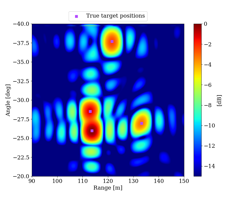
(a) Ideal conditions

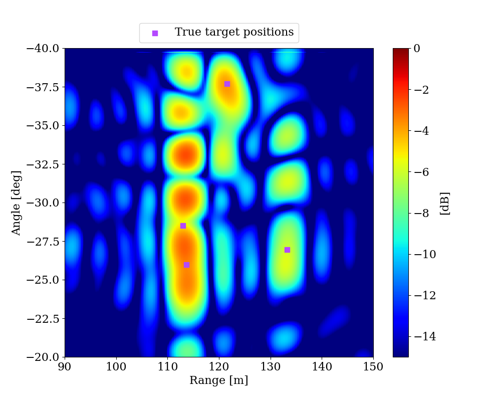
(b) Hardware impairments

Figure 3: Example of the angle-delay map when $T=4$ targets are present, under ideal conditions (top) and hardware impairments in the form of inter-antenna spacing mismatch (bottom), for an integrated sensing SNR of 20 dB. Both maps are normalized with respect to the maximum value of the angle-delay map under ideal conditions. More details about the specific simulation parameters can be found in Sec. V-A.

III Baseline

In this section, we derive the baseline method according to model-based benchmarks, which will later be compared with end-to-end learning approaches in Sec. V.

III-A ISAC Beamformer

We design the baseline for the precoding mapping in Fig. 2, which affects both the sensing precoder $\bm{f}_{r}$, and the communication precoder $\bm{f}_{c}$ in (5), by resorting to the beampattern synthesis approach in [56, 57]. We define a uniform angular grid covering $[-\pi/2,\pi/2]$ with $N_{\theta}$ grid locations $\{\theta_{i}\}_{i=1}^{N_{\theta}}$. For a given angular interval $\bm{\theta}_{\rm{interval}}$ (i.e., $\bm{\theta}_{\rm{interval}}=[\varphi_{\min},\varphi_{\max}]$ for communications, and $\bm{\theta}_{\rm{interval}}=[\theta_{\min},\theta_{\max}]$ for sensing), we denote by $\bm{b}\in\mathbb{C}^{N_{\theta}\times 1}$ the desired beampattern over the defined angular grid, given by

$$[\bm{b}]_{i}=\begin{cases}K,&~{}~{}\text{if}~{}~{}\theta_{i}\in\bm{\theta}_{\text{interval}}\\ 0,&~{}~{}\text{otherwise.}\end{cases}$$ (6)

The problem of beampattern synthesis can then be formulated as $\mathop{\mathrm{min}}\limits_{\bm{f}_{\text{bs}}}\lVert\bm{b}-\bm{A}^{\top}\bm{f}_{\text{bs}}\rVert_{2}^{2}$, where $\bm{A}=[\bm{a}(\theta_{1})\,\ldots\,\bm{a}(\theta_{N_{\theta}})]\in\mathbb{C}^{K\times N_{\theta}}$ denotes the transmit steering matrix evaluated at the grid locations. This least-squares (LS) problem has a simple closed-form solution

$$\bm{f}_{\text{bs}}=(\bm{A}^{\ast}\bm{A}^{\top})^{-1}\bm{A}^{\ast}\bm{b},$$ (7)

which yields, after normalization according to the transmit power constraints, a communication-optimal beam $\bm{f}_{c}$ or a radar-optimal beam $\bm{f}_{r}$, which can then be used to compute the joint ISAC beam in (5).

III-B Multi-target Sensing Receiver

We propose to formulate the multi-target sensing problem based on the received signal $\bm{Y}_{r}$ in (3) as a sparse signal recovery problem [58] and employ the OMP algorithm [44, 59, 60] to solve it, which represents our model-based benchmark. To construct an overcomplete dictionary for OMP, we specify an angular grid $\{\theta_{i}\}_{i=1}^{N_{\theta}}$ and a delay grid $\{\tau_{j}\}_{j=1}^{N_{\tau}}$ depending on the region of interest for target detection (i.e., the a priori information $\{\theta_{\min},\theta_{\max},R_{\min},R_{\max}\}$). Then, a spatial-domain and a frequency-domain dictionary covering angular and delay grids can be constructed as

$$\mathbf{\Phi}_{a} =[\bm{a}(\theta_{1})~{}\cdots~{}\bm{a}(\theta_{N_{\theta}})]\in\mathbb{C}^{K\times N_{\theta}}~{},$$ (8a)

$$\mathbf{\Phi}_{d} =[\bm{\rho}(\tau_{1})~{}\cdots~{}\bm{\rho}(\tau_{N_{\tau}})]\in\mathbb{C}^{S\times N_{\tau}}~{}.$$ (8b)

Using (8), the problem of multi-target sensing based on the observation in (3) becomes a sparse recovery problem

$$\widetilde{\bm{Y}}_{r}=\sum_{i=1}^{N_{\theta}}\sum_{j=1}^{N_{\tau}}[\bm{S}]_{i,j}[\mathbf{\Phi}_{a}]_{:,i}([\mathbf{\Phi}_{d}]_{:,j})^{\top}+\bm{N}~{},$$ (9)

where $\bm{S}\in\mathbb{C}^{N_{\theta}\times N_{\tau}}$. Here, the goal is to estimate the $T$-sparse vector ${\rm{vec}}(\bm{S})\in\mathbb{C}^{N_{\theta}N_{\tau}\times 1}$ under the assumption $T\ll N_{\theta}N_{\tau}$. The baseline OMP algorithm [58, 60, 43] to solve this problem is summarized in Algorithm 1, which will serve as a foundation to the proposed MB-ML approaches in Sec. IV-B.

Algorithm 1 Baseline OMP for Multi-Target Sensing

1:Input: Observation $\widetilde{\bm{Y}}_{r}$ in (3), dictionaries $\mathbf{\Phi}_{a}$ and $\mathbf{\Phi}_{d}$ in (8), termination threshold $\delta$.

2:Output: Set $\mathcal{A}$, which contains the angle and delay estimates of multiple targets $\{(\widehat{\theta}_{t},\widehat{\tau}_{t})\}_{t=1}^{I}$.

3:Initialization: Set $I=0$, $\mathcal{A}=\varnothing$, $\mathbf{\Psi}_{a}=\mathbf{\Psi}_{d}=[~{}]$.

4:Set the residual to $\widetilde{\bm{Y}}_{r}^{(0)}=\widetilde{\bm{Y}}_{r}$.

5:Compute angle-delay map $\mathcal{L}_{i,j}(\widetilde{\bm{Y}}_{r}^{(I)})=\big{\lvert}[\mathbf{\Phi}_{a}]_{:,i}^{H}\widetilde{\bm{Y}}_{r}^{(I)}[\mathbf{\Phi}_{d}]^{\ast}_{:,j}\big{\rvert}^{2}$.

6:while $\max_{i,j}\mathcal{L}_{i,j}(\widetilde{\bm{Y}}_{r}^{(I)})>\delta$

7:      Angle-delay detection:

$$(\hat{i},\hat{j})=\arg\max_{i,j}\mathcal{L}_{i,j}(\widetilde{\bm{Y}}_{r}^{(I)})~{}.$$ (10)

8:      Update angle-delay pairs: $\mathcal{A}\leftarrow\mathcal{A}\cup\{(\theta_{\hat{i}},\tau_{\hat{j}})\}$.

9:      Update atom sets:

$$\mathbf{\Psi}_{a} \leftarrow[\mathbf{\Psi}_{a}~{}[\mathbf{\Phi}_{a}]_{:,\hat{i}}]~{},$$ (11)

$$\mathbf{\Psi}_{d} \leftarrow[\mathbf{\Psi}_{d}~{}[\mathbf{\Phi}_{d}]_{:,\hat{j}}]~{}.$$ (12)

10:      Update gain estimates:

$$\widehat{\bm{\alpha}}=\arg\min_{\bm{\alpha}}\Big{\lVert}\widetilde{\bm{Y}}_{r}-\sum_{t=1}^{I+1}\alpha_{t}[\mathbf{\Psi}_{a}]_{:,t}([\mathbf{\Psi}_{d}]_{:,t})^{\top}\Big{\rVert}_{F}^{2}~{}.$$ (13)

11:     Update residual:

$$\widetilde{\bm{Y}}_{r}^{(I+1)}=\widetilde{\bm{Y}}_{r}-\sum_{t=1}^{I+1}\widehat{\alpha}_{t}[\mathbf{\Psi}_{a}]_{:,t}([\mathbf{\Psi}_{d}]_{:,t})^{\top}~{}.$$ (14)

12:      $I=I+1$.

13:end while

III-C Communication Receiver

We assume that the communication receiver has access to the CSI $\bm{\kappa}=\bm{\beta}\bm{f}^{\top}\bm{a}(\varphi)$. Hence, the received signal can be expressed as $\bm{y_{c}}=\bm{\kappa}\odot\bm{x}(\bm{m})+\bm{n}$. Optimal decoding in this case corresponds to subcarrier-wise maximum likelihood estimation according to

$$\widehat{m}_{s}=\arg\min_{m_{s}\in\mathcal{M}}\lvert[\bm{y_{c}}]_{s}-[\bm{\kappa}]_{s}x(m_{s})\rvert^{2},$$ (15)

for $s=0,...,S-1$. Since communication decoding is already optimal, given the CSI, learning methods described in Sec. IV apply (15) for communication message estimation.

IV Model-based Learning

[width=0.65mode=buildnew]figures/omp_1_iteration

Figure 4: Block diagram of the $I$-th iteration of the differentiable OMP algorithm for model-based learning. Continuous lines indicate where the gradient of the loss function flows during backpropagation. Colored blocks highlight modified operations with respect to conventional OMP. The algorithm stops when $\max_{i,j}\mathcal{L}_{i,j}(\widetilde{\bm{Y}}_{r}^{(I)})$ drops below a threshold.

MB-ML is inspired by the baseline of Sec. III, although we need to develop differentiable beamforming and estimation algorithms that permit end-to-end learning, as well as a suitable loss function for multiple targets. This section describes the two MB-ML methods developed for multi-target sensing: (i) dictionary learning, which learns a dictionary of steering vectors for different angles as in [46], and is suitable for unstructured impairments, as defined in Sec. II-D; (ii) impairment learning, which directly learns a parameterization of the hardware impairments and thus is suitable for structured impairments, also defined in Sec. II-D. This section also defines the loss function to train them.

IV-A Beamformer

MB-ML follows the same operations (6) and (7) to compute the precoding vector $\bm{f}_{r}$ or $\bm{f}_{c}$, given an angular interval $\bm{\theta}_{\rm{interval}}$. Dictionary learning considers $\bm{A}\in\mathbb{C}^{K\times N_{\theta}}$ from (7) as a free learnable parameter to account for unstructured impairments, which is comprised of $KN_{\theta}$ complex parameters.

The new proposed impairment learning considers instead as a free learnable parameter the vector $\bm{d}\in\mathbb{C}^{K}$, which represents a parameterization of the structured hardware impairments. From $\bm{d}$, the dictionary of steering vectors is computed as $\bm{A}_{\rm{pert}}(\bm{d})=[\bm{a}_{\rm{pert}}(\theta_{1};\bm{d})\,\ldots\,\bm{a}_{\rm{pert}}(\theta_{N_{\rm{grid}}};\bm{d})]$, such that $\bm{A}_{\rm{pert}}(\bm{d})$ is used in (7) instead of $\bm{A}$. Impairment learning reduces the number of learnable parameters by taking into account the structured hardware impairments of Sec. II-D. Indeed, it has only $K$ complex parameters, which can be several order of magnitudes less than the dictionary learning approach, since the dictionary of steering vector needs a relatively large number of columns $N_{\theta}$ to perform well. Note that the operation in (7), which involves the learning parameters of both MB-ML methods, is already differentiable.

IV-B Sensing Receiver

Range-angle estimation of targets is based on Algorithm 1. However, the $\arg\max$ operation in line 7 of Algorithm 1 is not differentiable and the gradient of no loss function could be backpropagated in MB-ML. To circumvent this issue, we develop a differentiable algorithm which is represented in Fig. 4. The difference with the conventional OMP in Algorithm 1 is that we replace the operations of lines 7-9 by the following steps:

1. $\arg\max_{i,j}\mathcal{L}_{i,j}(\widetilde{\bm{Y}}_{r}^{(I)})$: We still perform this nondifferentiable operation as a temporary result to obtain the final estimation. Note that $\mathcal{L}_{i,j}(\widetilde{\bm{Y}}_{r}^{(I)})$ is based on an angular grid $\bm{\theta}_{\rm{grid}}=\{\theta_{i}\}_{i=1}^{N_{\theta}}$ and a delay grid $\bm{\tau}_{\text{grid}}=\{\tau_{j}\}_{j=1}^{N_{\tau}}$. In line 7 in Algorithm 1, this calculation yields the estimated angle-delay pair, which serves as foundation for the following step of the differentiable OMP algorithm.

2. Mask the angle-delay map, $\mathcal{L}_{i,j}(\widetilde{\bm{Y}}_{r}^{(I)})$, based on angle and range resolution: in order to consider elements of $\mathcal{L}_{i,j}(\widetilde{\bm{Y}}_{r}^{(I)})$ that solely correspond to a single target, we select the elements around the maximum of the angle-delay map that are within the angle and range resolution. This operation also helps to obtain a differentiable angle-delay estimation, similar to line 7 in Algorithm 1. We create the mask based on the angle and range resolution, since it determines the minimum angle or range for which two targets are indistinguishable. The angle and range resolutions in our case are

   $$\delta_{\theta}\approx\frac{2}{K}\quad\delta_{R}\approx\frac{c}{2B}=\frac{c}{2S\Delta_{f}},$$ (16)

   with $B$ the bandwidth of the transmitted signal. The resolutions are considered in terms of the number of pixels of the angle-delay map, depending on $N_{\theta}$ and $N_{\tau}$.

3. Softmax: We apply a softmax operation to the masked matrix from the previous operation, so that the sum of its elements is equal to 1. Unlike line 7 in Algorithm 1, the softmax function is differentiable, enabling end-to-end learning.

4. Weighted sum: A weighted sum of $\bm{\theta}_{\rm{grid}}$ and $\bm{\tau}_{\text{grid}}$ is implemented, where each weight corresponds to the output of the previous softmax operation, and they represent an estimate of the probability that a certain angle-delay pair is the true value. From this interpolation operation, an angle-delay pair $(\hat{\theta}_{I},\hat{\tau}_{I})$ is obtained, which may not be included in $\bm{\theta}_{\rm{grid}}$ or $\bm{\tau}_{\text{grid}}$. From this computation, the angle-delay pairs are updated, as in line 8 in Algorithm 1. Note that these four first steps (center column of Fig. 4), amount to looking in the dictionary for the most correlated atoms with the input, and then estimating the angle-delay pair as a convex combination of the corresponding angle-delays on the grid. This kind of similarity-based learning has been applied to other tasks within MIMO systems [61], and is reminiscent of the attention mechanism [62].

5. Compute estimated spatial-domain and frequency-domain vectors $\bm{a}(\hat{\theta}_{I})$, $\bm{\rho}(\hat{\tau}_{I})$: unlike line 9 in Algorithm 1, we recompute the spatial-domain and frequency-domain vectors based on the estimated angle-delay pair of the previous step, since the estimated angle-delay pair $(\widehat{\theta}_{I},\widehat{\tau}_{I})$ might not be contained in $(\bm{\theta}_{\rm{grid}},\bm{\tau}_{\text{grid}})$. The sets $\mathbf{\Psi}_{a}$ and $\mathbf{\Psi}_{d}$ are updated with the new vectors, as represented in Fig. 4.

After the previous steps, differentiable OMP continues as lines 10-12 in Algorithm 1 to obtain the new residual $\widetilde{\bm{Y}}_{r}^{(I+1)}$, as depicted in Fig. 4. This differentiable OMP algorithm still involves looking over a grid of possible angles. We utilize as the dictionary of angles $\mathbf{\Phi}_{a}$ the same matrices $\bm{A}$ and $\bm{A}_{\rm{pert}}(\bm{d})$ from the beamformer of Sec. IV-A to compute $\mathcal{L}_{i,j}(\widetilde{\bm{Y}}_{r}^{(I)})$, which allows parameter sharing between the co-located transmitter and receiver. The gradient of the loss function does not flow through the $\arg\max$ operation, as illustrated in Fig. 4. To further improve memory efficiency, gradient flow is also discarded when computing the new residual $\widetilde{\bm{Y}}_{r}^{(I+1)}$ from the estimates $(\widehat{\theta}_{I},\widehat{\tau}_{I})$.

IV-C Loss Function

As loss function for MB-ML multi-target sensing, we select the generalized optimal sub-pattern assignment (GOSPA) loss from [63]. In our case, the GOSPA loss is defined as follows. Let $\gamma>0$, $0<\mu\leq 2$ and $1\leq p<\infty$. Let $\mathcal{P}=\{\bm{p}_{1},...,\bm{p}_{|\mathcal{P}|}\}$ and $\hat{\mathcal{P}}=\{\hat{\bm{p}}_{1},...,\hat{\bm{p}}_{|\hat{\mathcal{P}}|}\}$ be the finite subsets of $\mathbb{R}^{2}$ corresponding to the true and estimated target positions, respectively, with $0\leq|\mathcal{P}|\leq T_{\rm{max}}$, $0\leq|\hat{\mathcal{P}}|\leq T_{\rm{max}}$. Let $d(\bm{p},\hat{\bm{p}})=\lVert\bm{p}-\hat{\bm{p}}\rVert_{2}$ be the distance between true and estimated positions, and $d^{(\gamma)}(\bm{p},\hat{\bm{p}})=\min(d(\bm{p},\hat{\bm{p}}),\gamma)$ be the cut-off distance. Let $\Pi_{n}$ be the set of all permutations of $\{1,...,n\}$ for any $n\in\mathbb{N}$ and any element $\pi\in\Pi_{n}$ be a sequence $(\pi(1),...,\pi(n))$. For $|\mathcal{P}|\leq|\hat{\mathcal{P}}|$, the GOSPA loss function is defined as

$$d_{p}^{(\gamma,\mu)}(\mathcal{P},\hat{\mathcal{P}})=$$

$$\bigg{(}\min_{\pi\in\Pi_{|\hat{\mathcal{P}}|}}\sum_{i=1}^{|\mathcal{P}|}d^{(\gamma)}(\bm{p}_{i},\hat{\bm{p}}_{\pi(i)})^{p}+\frac{\gamma^{p}}{\mu}(\lvert\hat{\mathcal{P}}\rvert-\lvert\mathcal{P}\rvert)\bigg{)}^{\frac{1}{p}}.$$ (17)

If $\lvert\mathcal{P}\rvert>\lvert\hat{\mathcal{P}}\rvert,d_{p}^{(\gamma,\mu)}(\mathcal{P},\hat{\mathcal{P}})=d_{p}^{(\gamma,\mu)}(\hat{\mathcal{P}},\mathcal{P})$. The parameter $p$ is proportional to the penalization of outliers, and the value of $\gamma$ dictates the maximum allowable distance error. The role of $\mu$, together with $\gamma$, is to control the detection penalization. This loss function becomes suitable for multiple targets, since it considers the association between estimated and true positions that gives the minimum loss, tackling the data association problem of multiple targets. In terms of target detection, we follow the same principle as the baseline, i.e., we stop the OMP algorithm when the maximum of the angle-delay map drops below a threshold. Sweeping this threshold over different values yields a trade-off in terms of detection and false alarm rates.

V Results

This section details the simulation parameters and the results for single- and multi-target ISAC. Four methods will be evaluated and compared:

• The model-based baseline from Sec. III, working under the mismatched assumption of no hardware impairments.

• A NNBL method, extending [34, 35], which replaces the precoding and sensing estimation mappings in Fig. 2 by NNs, and can operate in the absence of any knowledge of the ISAC system (including the hardware impairments). More details can be found in Appendix A.

• Dictionary learning from Sec. IV, where the unstructured impaired steering vectors $\bm{a}_{\rm{pert}}(\theta)$ are learned for both precoding and sensing.

• Impairment learning from Sec. IV, where the structured impairment vector $\bm{d}$ is learned for precoding and sensing.

V-A Simulation Parameters

We consider a ULA of $K=64$ antennas, $S=256$ subcarriers, and a subcarrier spacing of $120$ kHz. We set the maximum number of targets in the scene as $T_{\rm{max}}=5$. The transmitted power is $P=1$ and the carrier frequency is $f_{c}=60$ GHz. The sensing SNR across antenna elements was set to $\text{SNR}_{r}=K\sigma_{r}^{2}/N_{0}=15$ dB, and the average communication SNR per subcarrier was fixed to $\text{SNR}_{c}=\sum_{l=1}^{L}\sigma_{c,l}^{2}/(SN_{0})=20$ dB. The number of channel taps in the communication channel is $L=5$, with an exponential power delay profile, i.e., $\sigma_{l}^{2}=\exp{(-l)},l=0,...,L-1$. The power delay profile is later normalized to obtain the desired average SNR. The number of grid points for angle and range is set as $N_{\theta}=720$ and $N_{\tau}=200$.

To train the learning methods for a wide range of angles, we randomly draw $\{\theta_{\min},\theta_{\max}\}$ as in [64], i.e., we draw a realization of $\theta_{\text{mean}}\sim\mathcal{U}[-60^{\circ},60^{\circ}]$ and $\Delta\sim\mathcal{U}[10^{\circ},20^{\circ}]$, for each new transmission. The target angular sector is computed as $\theta_{\min}=\theta_{\text{mean}}~{}-~{}\Delta/2$, $\theta_{\max}=\theta_{\text{mean}}~{}+~{}\Delta/2$. The communication angular sector and the range uncertainty region are set as $\{\varphi_{\min},\varphi_{\max}\}=\{30^{\circ},50^{\circ}\}$, $\{R_{\min},R_{\max}\}=\{10,190\}$ m, for all transmissions. For hardware impairments, we consider the model of [34, 64], i.e., we assume structured hardware impairments where the antenna elements in the ULA array are spaced as $\bm{d}\sim\mathcal{CN}((\lambda/2)\bm{1},\sigma_{\lambda}^{2}\bm{I}_{K})$. We select a standard deviation of $\sigma_{\lambda}=\lambda/25=0.2$ mm. MB-ML is initialized with the same knowledge as the baseline, i.e., the steering vector models firstly assume that $d=(\lambda/2)\bm{1}$.

In the GOSPA loss, we set $\mu=2$, as recommended in [63], $p=2$, and $\gamma=(R_{\max}-R_{\min})/2=90$ m. The cardinality mismatch term in (17) implies the use of a threshold during training. However, our goal is to train the learning methods regardless of the threshold, and then explore sensing performance by changing the threshold. Hence, during training it is assumed to know the actual number of targets $T$, which means that $|\mathcal{P}|=|\hat{\mathcal{P}}|=T$, and the GOSPA loss during training becomes

$$d_{p}^{(\gamma,\mu)}(\mathcal{P},\hat{\mathcal{P}})=\bigg{(}\min_{\pi\in\Pi_{|\hat{\mathcal{P}}|}}\sum_{i=1}^{|\mathcal{P}|}d^{(\gamma)}(\bm{p}_{i},\hat{\bm{p}}_{\pi(i)})^{p}\bigg{)}^{\frac{1}{p}}.$$ (18)

However, there is no detection penalization term in (18), which implies that the detection probability estimation NN of NNBL cannot be optimized. Hence, we adopt a two-step training approach for NNBL, as follows:

1. We first train $f_{\bm{\varepsilon}}$ and $f_{\bm{\xi}}$ based on the simplified GOSPA loss of (18).

2. While freezing the parameters $\bm{\xi}$, we then train $f_{\bm{\varepsilon}}$ and $f_{\bm{\zeta}}$ by minimizing

   $$d_{u}^{(\gamma_{u},\mu)}(\mathcal{D},\hat{\mathcal{D}})=\bigg{(}\min_{\pi\in\Pi_{|\hat{\mathcal{D}}|}}\sum_{i=1}^{|\mathcal{D}|}d^{(\gamma_{u})}(u_{i},\hat{u}_{\pi(i)})^{p}\bigg{)}^{\frac{1}{p}},$$ (19)

   where $\mathcal{D}=\{u_{1},...,u_{|\mathcal{D}|}\}$ and $\hat{\mathcal{D}}=\{\hat{u}_{1},...,\hat{u}_{|\hat{\mathcal{D}}|}\}$ are the true and estimated sets of target probabilities, $d^{(\gamma_{u})}(u_{i},\hat{u}_{\pi(i)})=\min(d(u_{i},\hat{u}_{\pi(i)}),\gamma_{u})$, and $d(u_{i},\hat{u}_{\pi(i)})=-u_{i}\log(\hat{u}_{\pi(i)})-(1-u_{i})\log(1-\hat{u}_{\pi(i)})$. That is, we replace the position distance error in (18) with the binary cross-entropy (BCE) loss. Note that in (19) we also assume that $|\mathcal{D}|=|\hat{\mathcal{D}}|=T$.

The previous two-step training approach was observed to yield better performance, compared to joint training of all NN parameters $\bm{\varepsilon},\bm{\xi},\bm{\zeta}$ based on the sum of the losses (18) and (19).

Network optimization is performed using the Adam optimizer [65], with a batch size of $B=3000$ and 100,000 training iterations. The learning rate of dictionary and impairment learning was set to $5\cdot 10^{-3}$ and $10^{-7}$, respectively. In the two-step training approach for NNBL, 100,000 training iterations are applied to each of the steps. Position estimation training used a learning rate of $10^{-2}$, while target detection utilized $10^{-3}$ as learning rate. The architecture of NNBL is described in Appendix A-B. NNBL also benefited from using a scheduler, to reduce the learning rate when the loss function has reached a plateau. Details of the scheduler parameters can be found in Appendix A-B.

V-B Performance Metrics

Concerning testing, we compute as detection performance metrics a measure of the probability of misdetection and the probability of false alarm, for multiple targets. We use the same definitions as in [35], which correspond to

$$p_{\text{md}}=1-\frac{\sum_{i=1}^{B}\min\{T_{i},\widehat{T}_{i}\}}{\sum_{i=1}^{B}T_{i}},$$ (20)

$$p_{\text{fa}}=\frac{\sum_{i=1}^{B}\max\{T_{i},\widehat{T}_{i}\}-T_{i}}{\sum_{i=1}^{B}T_{\rm{max}}-T_{i}},$$ (21)

where $T_{i}$, $\widehat{T}_{i}$ are the true and estimated number of targets in each batch sample, respectively. The regression performance is measured via the GOSPA (for multiple targets sensing) and root mean squared error (RMSE) (for single target sensing).

As communication performance metric, we use the average symbol error rate (SER) across subcarriers, computed as

$$\text{SER}=\frac{1}{BS}\sum_{i=1}^{B}\sum_{j=1}^{S}\mathbb{I}\{[\bm{m}_{i}]_{j}\neq[\hat{\bm{m}}_{i}]_{j}\},$$ (22)

with $\bm{m}_{i}$ and $\hat{\bm{m}}_{i}$ the true and estimated message vectors at the $i$-th batch sample. All described methods in this paper (baseline of Sec. III, MB-ML of Sec. IV, and NNBL) use a quadrature phase shift keying (QPSK) encoder, and the message estimation rule in (15).

V-C Single-target ISAC

In single-target ISAC, the maximum number of targets is $T_{\rm{max}}=1$, which implies that the GOSPA loss function in (18) becomes $d^{(\gamma)}(\bm{p},\hat{\bm{p}})$. However, in order to compare with our previous work [46], we train MB-ML and position estimation of NNBL using the mean squared error (MSE) loss $d(\bm{p},\hat{\bm{p}})^{p}=\|\bm{p}-\hat{\bm{p}}\|_{2}^{2}$, and detection estimation of NNBL using the BCE loss, $d(u,\hat{u})=-u\log(\hat{u})-(1-u)\log(1-\hat{u})$. Position estimation is assessed by the angle RMSE, $\sqrt{\mathbb{E}[(\theta-\hat{\theta})^{2}]}$, and the range RMSE, $\sqrt{\mathbb{E}[(R-\hat{R})^{2}]}$.

ISAC performance results are represented in Fig. 5, where we sweep over $[0,1]$ and $[0,7\pi/4]$, taking 8 uniformly spaced values, to set $\eta$ and $\phi$ in (5), respectively. For testing, we fixed $\{\theta_{\min},\theta_{\max}\}=\{-40^{\circ},-20^{\circ}\}$. The probability of false alarm was set to $p_{\text{fa}}=10^{-2}$.

[width=0.5mode=buildnew]result_figures/isac_single_target

Figure 5: Single-target ISAC trade-offs under hardware impairments.

Result show that under no complexity limitations (solid lines) and hardware impairments, learning methods outperform the baseline in terms of misdetection probability, angle and range estimation, and SER, which implies that learning methods have adapted to hardware impairments. Communication performance, even in the case of optimal symbol estimation, is enhanced by learning approaches, which suggests that the impairments have a significant impact on the optimal communication precoder. In addition, dictionary learning outperforms NNBL for range estimation, although the converse happens for misdetection probability. Impairment learning yields the best performance among all learning methods, and with fewer parameters, which usually implies less training time. Indeed, NNBL is composed of a total of 7.78 million real learnable parameters, while dictionary learning uses $KN_{\theta}=40,080$ complex parameters, and impairment learning consists of $K=64$ complex parameters.

Under limited complexity, the number of parameters of dictionary learning and NNBL are restricted. We follow the approach of [34], and restrict the number of (complex) parameters of dictionary learning by setting $N_{\theta}=156$, which reduces the number of parameters to 9,984 complex parameters. The complexity constraints applied to NNBL-learning are detailed in Appendix A-B, which decreases the number of real parameters to 10,555. From Fig. 5, it is observed that while NNBL drops in performance, especially for angle and range estimation, dictionary learning still yields better results than the baseline. However, dictionary learning also decreased in performance compared to the unconstrained approach, which means that dictionary learning cannot achieve the same performance as impairment learning for the same number of parameters.

Lastly, we test all learning approaches for a scenario that was not encountered during training, to assess their generalization capabilities. Fig. 6 depicts the performance of the learning methods for $\{\theta_{\min},\theta_{\max}\}=\{-20^{\circ},20^{\circ}\}$, which includes a span of the angular uncertainty region wider than expected. The complexity of the networks is not restricted. The performance of all learning approaches has dropped compared to Fig. 5. However, while NNBL performs worse than the baseline, and dictionary learning yields similar results to the baseline, impairment learning is the only approach that still outperforms the baseline. NNBL and dictionary learning appear to overfit to the training data and degrade for unexpected inputs. This means that for new testing scenarios, impairment learning is the learning approach that best generalizes in terms of performance. This is due to the fact that impairment learning is the only method for which parameters are shared between all directions (all columns of the dictionary are affected each time the parameters are updated). Dictionary learning does not exhibit this feature, since each column of the dictionary (corresponding to a direction) is considered an independent set of parameters.

[width=0.5mode=buildnew]result_figures/isac_single_target_unseen

Figure 6: Single-target ISAC generalization trade-offs under hardware impairments and new (unseen) testing data. The target lies in the angular sector $\{\theta_{\min},\theta_{\max}\}=\{-20^{\circ},20^{\circ}\}$. The complexity of the networks is not limited.

V-D Multi-target ISAC

Based on the results of Sec. V-C, impairment learning performs the best among all considered learning methods for the simpler case of single-target ISAC. Hence, we only consider impairment learning to compare against the baseline for multi-target sensing. The batch size for MB-ML is decreased to $B=1500$ due to memory restrictions. The number of iterations was also reduced to 25,000, since finding the association between estimated and true data that minimizes the GOSPA loss of (18) increases training time. In addition, ISAC results perform very close to perfect knowledge of impairments, as observed in the following.

We first compare the performance of the differentiable OMP algorithm of Sec. IV-B with the baseline, when hardware impairments are perfectly known. In Fig. 7, the sensing performance of both approaches is depicted. Results show that differentiable OMP performs closely to the baseline. The difference in performance might be because the dictionary $\mathbf{\Phi}_{a}$ in the baseline only covers the angular range $\{\theta_{\min},\theta_{\max}\}$, while differentiable OMP uses a fixed dictionary that covers $[-\pi/2,\pi/2]$. However, this allows for efficient parameter sharing in MB-ML. Differentiable OMP takes a weighted sum of angles and ranges, which permits to select an angle or range outside the predefined dictionaries, unlike the baseline. The GOSPA loss in Fig. 7 achieves a minimum for different false alarm probabilities, since it takes into account both position and detection errors. For high $p_{\text{fa}}$, OMP estimates a higher number of targets than the true value, and conversely for low $p_{\text{fa}}$.

[width=0.5mode=buildnew]result_figures/multi_target_roc_omp

Figure 7: Sensing performance for standard and differentiable OMP algorithms, when perfect impairment knowledge is available. The transmitter in both cases is implemented as the baseline of Sec.III-A.

Fig. 8 shows the results of the baseline without impairment knowledge, differentiable OMP with perfect impairment knowledge, and impairment learning. Impairment learning outperforms the baseline, which illustrates the adaptability of impairment learning to antenna imperfections in multi-target sensing. Moreover, the performance is very close to perfect knowledge of the impairments, which suggests that the learned spacing is quite similar to the underlying reality.

[width=0.5mode=buildnew]result_figures/multi_target_roc_hwi

Figure 8: Sensing performance of diffferentiable OMP and impairment learning. The transmitter of differentiable OMP is implemented as the baseline of Sec.III-A.

In terms of ISAC trade-off, Fig. 9 presents the ISAC trade-offs in case of multiple targets when $p_{\text{fa}}=10^{-2}$. In this case, we sweep in (5) over $\eta$ and fixed $\phi=0$, since in Figs.5 and 6 we observed that the effect of $\phi$ is not very significant. Compared to Fig. 8, it is observed that impairment learning also outperforms the baseline when impairments are not known in terms of communication performance, due to the impact of hardware impairments in the communication precoder.

[width=0.5mode=buildnew]result_figures/multi_target_isac

Figure 9: Multi-target ISAC trade-offs, when the false alarm probability is set to $10^{-2}$. The transmitter of differentiable OMP is implemented as the baseline of Sec.III-A.

VI Conclusions

In this work, we studied the effect of antenna spacing impairments in multi-target ISAC, and different learning approaches to compensate for such impairments. A new efficient MB-ML approach to perform end-to-end learning and impairment compensation was proposed, based on a differentiable OMP algorithm. Simulation results showed that learning approaches outperform the baseline and they can compensate for hardware impairments. Among learning methods, the new proposed impairment learning approach outperformed all other considered methods, also exhibiting better generalization capabilities to new testing data, with much fewer parameters to optimize. Simulations results verify that injection of the system and impairment knowledge in learning methods improves their performance and reduces their complexity.

Appendix A neural-network-based learning (NNBL)

Since the optimal detection and estimation rules might not be tractable, NNBL can be trained based on data to achieve optimality. Moreover, when no information about the impairments is available, NNBL can provide data-driven solutions to account for them. This appendix describes the principles and architecture of the considered NNBL approach.

A-A Principles

NNBL replaces the precoding and sensing estimation mappings in Fig. 2 by NNs. The precoding network, $f_{\bm{\varepsilon}}:\mathbb{R}^{2}\to\mathbb{R}^{2K}$, takes $\bm{\theta}_{\rm{interval}}$ as input and produces a precoder as output, where $\bm{\varepsilon}$ corresponds to the learnable parameters. NN in this work are considered to work with real-valued numbers, hence, the output dimension is doubled. The same mapping $f_{\bm{\varepsilon}}$ is applied to both sensing and communication precoders, to obtain $\bm{f}_{r}$ and $\bm{f}_{c}$, which are later used to design the ISAC precoder according to (5).

Sensing estimation is divided into two tasks, each corresponding to a different NN: (i) detection probability estimation, and (ii) position estimation. As input to both NNs, we use $\mathcal{L}_{i,j}(\widetilde{\bm{Y}}_{r}^{(I)})\in\mathbb{R}^{N_{\theta}\times N_{\tau}}$ defined in Sec. III, instead of $\widetilde{\bm{Y}}_{r}$, since we observed a better sensing performance. In addition to the angle-delay map, the input is also composed of the a priori information $\{\theta_{\min},\theta_{\max},R_{\min},R_{\max}\}$, as shown in Fig 2, to improve network performance. The output of each NN is task-dependent. The detection probability network, $f_{\bm{\zeta}}:\mathbb{R}^{N_{\theta}\times N_{\tau}}\times\mathbb{R}^{4}\to[0,1]^{T_{\rm{max}}}$, outputs a probability vector $\hat{\bm{u}}$ whose elements correspond to the probability that each target is present in the scene, which is later thresholded to provide an estimate of the number of targets. The position estimation network, $f_{\bm{\xi}}:\mathbb{R}^{N_{\theta}\times N_{\tau}}\times\mathbb{R}^{4}\to\mathbb{R}^{T_{\rm{max}}\times 2}$, outputs a matrix $\hat{\bm{P}}$ whose columns represent the position estimation of each potential target. The learnable parameters of each network are $\bm{\zeta}$ and $\bm{\xi}$, respectively. Both NNs are trained based on the GOSPA loss function of Sec. IV-C.

A-B NN Architectures

The precoding operation of Fig. 2 was implemented as a multilayer perceptron (MLP), whose input is an angular sector ($\{\theta_{\min},\theta_{\max}\}$ or $\{\varphi_{\min},\varphi_{\max}\}$), with 3 hidden layers of $8K$ neurons and an output layer of $2K$ neurons, where we recall that $K=64$ is the number of antennas in the ULA transceiver. The activation function after each layer is the Rectified Linear Unit (ReLU) function, except for the final layer, which contains a normalization layer to ensure a unit-norm output, i.e., $\lVert\bm{f}_{\text{bs}}\rVert_{2}=1$.

For the receiver side, we resort to convolutional neural networks given the 2-dimensional nature of the input $\mathcal{L}_{i,j}(\widetilde{\bm{Y}}_{r}^{(I)})$, as represented in Fig. 3. The receiver architecture repeats a set of layers, represented in Fig. 10, which we call residual bottleneck block. This block was inspired by the ResNet architecture [66]. A convolutional layer is first introduced with some stride to decrease the number of pixels to process. Then, 2 bottleneck blocks with skipped connections similar to [66] follow. However, we reduce the number of activation functions and normalization layers, as suggested in [67]. Another residual connection is introduced from the beginning to the end of both bottleneck blocks to help with gradient computation.

[width=0.45mode=buildnew]figures/residual_bottleneck_v2

Figure 10: Block diagram of the residual bottleneck block with $C_{\text{in}}$ input channels and $C_{\text{out}}$ output channels.

We observed that splitting position estimation into angle and range estimation, each of them involving a CNN, yielded better results than using a single network. Angle and range estimates are later combined into a position vector following (2). The common architecture for all CNNs (detection, angle and range estimation) is shown in Table I. Convolutional layers introduce zero-padding so that the number of pixels is preserved. After the first and last convolutional layers, a 2-dimensional batch normalization and a ReLU activation function are also applied. The resulting feature map of the CNN has $N_{\theta}N_{\tau}/2^{12}$ elements. For NNBL, $N_{\theta}=320$ and $N_{\tau}=128$ due to memory constraints. The resulting feature map from the convolutional layers, together with the a priori information $\{\theta_{\min},\theta_{\max},R_{\min},R_{\max}\}$ of the target locations, are processed by MLPs. The angle estimation network only uses $\{\theta_{\min},\theta_{\max}\}$, the range estimation network $\{R_{\min},R_{\max}\}$, and the detection network utilizes both of them. The architecture of each MLP is described in Table II. The activation function after each fully-connected layer is the ReLU function. Unless stated otherwise, all NN architectures were optimized to give the best ISAC performance, where we explored, for instance, kernel sizes up to 13x13, the number of residual bottleneck blocks from 3 to 7, or the number of layers of the MLP of Table II, from $K$ to $64K$, among others.

TABLE I: Common architecture of the convolutional neural networks.

Layer type	Kernel Size	Stride	In. CHs	Out. CHs
Convolutional	5x5	1	1	8
Maxpool	2x2	-	8	8
Residual Bottleneck	3x3	1	8	16
Residual Bottleneck	3x3	2	16	32
Residual Bottleneck	3x3	2	32	64
Residual Bottleneck	3x3	2	64	128
Residual Bottleneck	3x3	2	128	256
Residual Bottleneck	3x3	2	256	512
Convolutional	3x3	1	512	1

TABLE II: Multi-layer perceptron architecture for each task.

Task	Input layer	Hidden layers	Output layer
Angle estimation	$\frac{N_{\theta}N_{\tau}}{2^{12}}$	($4K$, $4K$)	1 (tanh$\cdot 90$)
Range estimation			1 (ReLU)
Target detection			1 (sigmoid)

When training NNBL, a scheduler is used to reduce the learning rate if the loss function plateaus. The patience of the scheduler was set as $10^{4}$ iterations. If the loss function was regarded to plateau, the learning rate was decreased by half, with a minimum attainable learning rate of $10^{-6}$.

When complexity limitations are considered, in the transmitter network the number of neurons in each hidden layer was reduced to 4. At the receiver side, the kernel size of the Maxpool layer is increased to 4x4, the number of residual bottleneck blocks is changed from 6 to 3, the number of channels in the network is reduced by a factor of 4, and the number of neurons in the hidden layer of the last MLP are constrained to 4.

References

- [1] C.-X. Wang, X. You, X. Gao, X. Zhu, Z. Li, C. Zhang, H. Wang, Y. Huang, Y. Chen, H. Haas, J. S. Thompson, E. G. Larsson, M. D. Renzo, W. Tong, P. Zhu, X. Shen, H. V. Poor, and L. Hanzo, “On the road to 6G: Visions, requirements, key technologies and testbeds,” IEEE Commun. Surveys & Tutorials, vol. 25, no. 2, pp. 905–974, Feb. 2023.
- [2] H. Tataria, M. Shafi, A. F. Molisch, M. Dohler, H. Sjöland, and F. Tufvesson, “6G wireless systems: Vision, requirements, challenges, insights, and opportunities,” Proc. IEEE, vol. 109, no. 7, pp. 1166–1199, Jul. 2021.
- [3] M. Matthaiou, O. Yurduseven, H. Q. Ngo, D. Morales-Jimenez, S. L. Cotton, and V. F. Fusco, “The road to 6G: Ten physical layer challenges for communications engineers,” IEEE Commun. Mag., vol. 59, no. 1, pp. 64–69, Feb. 2021.
- [4] W. Saad, M. Bennis, and M. Chen, “A vision of 6G wireless systems: Applications, trends, technologies, and open research problems,” IEEE Netw., vol. 34, no. 3, pp. 134–142, Oct. 2019.
- [5] A. R. Chiriyath, B. Paul, and D. W. Bliss, “Radar-communications convergence: Coexistence, cooperation, and co-design,” IEEE Trans. Cogn. Commun. Netw., vol. 3, no. 1, pp. 1–12, Feb. 2017.
- [6] D. K. P. Tan, J. He, Y. Li, A. Bayesteh, Y. Chen, P. Zhu, and W. Tong, “Integrated sensing and communication in 6G: Motivations, use cases, requirements, challenges and future directions,” in Proc. 1st IEEE Int. Symp. Joint Commun. & Sens. (JC&S), Dresden, Germany, 2021, pp. 1–6.
- [7] H. Wymeersch, D. Shrestha, C. M. De Lima, V. Yajnanarayana, B. Richerzhagen, M. F. Keskin, K. Schindhelm, A. Ramirez, A. Wolfgang, M. F. De Guzman et al., “Integration of communication and sensing in 6G: A joint industrial and academic perspective,” in Proc. 32nd IEEE Annu. Int. Symp. Personal Indoor Mobile Radio Commun. (PIMRC), Helsinki, Finland, 2021, pp. 1–7.
- [8] F. Liu, Y. Cui, C. Masouros, J. Xu, T. X. Han, Y. C. Eldar, and S. Buzzi, “Integrated sensing and communications: Towards dual-functional wireless networks for 6G and beyond,” IEEE J. Sel. Areas Commun., vol. 40, no. 6, pp. 1728–1767, Mar. 2022.
- [9] S. Lu, F. Liu, Y. Li, K. Zhang, H. Huang, J. Zou, X. Li, Y. Dong, F. Dong, J. Zhu et al., “Integrated sensing and communications: Recent advances and ten open challenges,” arXiv preprint arXiv:2305.00179, 2023.
- [10] F. Lampel, R. F. Tigrek, A. Alvarado, and F. M. Willems, “A performance enhancement technique for a joint FMCW RADCOM system,” in Proc. IEEE 16th Eur. Radar Conf. (EuRAD), Paris, France, 2019, pp. 169–172.
- [11] A. Lazaro, M. Lazaro, R. Villarino, D. Girbau, and P. de Paco, “Car2car communication using a modulated backscatter and automotive FMCW radar,” Sensors, vol. 21, no. 11, p. 3656, May 2021.
- [12] J. A. Zhang, M. L. Rahman, K. Wu, X. Huang, Y. J. Guo, S. Chen, and J. Yuan, “Enabling joint communication and radar sensing in mobile networks—a survey,” IEEE Commun. Surv. & Tut., vol. 24, no. 1, pp. 306–345, Oct. 2021.
- [13] L. Chen, F. Liu, W. Wang, and C. Masouros, “Joint radar-communication transmission: A generalized pareto optimization framework,” IEEE Trans. Signal Process., vol. 69, pp. 2752–2765, May 2021.
- [14] S. D. Liyanaarachchi, C. B. Barneto, T. Riihonen, M. Heino, and M. Valkama, “Joint multi-user communication and MIMO radar through full-duplex hybrid beamforming,” in Proc. 1st IEEE Int. Online Symp. Joint Commun. & Sens. (JC&S), Dresden, Germany, 2021, pp. 1–5.
- [15] S. H. Dokhanchi, M. B. Shankar, M. Alaee-Kerahroodi, and B. Ottersten, “Adaptive waveform design for automotive joint radar-communication systems,” IEEE Trans. Veh. Technol., vol. 70, no. 5, pp. 4273–4290, Apr. 2021.
- [16] J. Johnston, L. Venturino, E. Grossi, M. Lops, and X. Wang, “MIMO OFDM dual-function radar-communication under error rate and beampattern constraints,” IEEE J. Select. Areas Commun., vol. 40, no. 6, pp. 1951–1964, Mar. 2022.
- [17] F. Liu, L. Zhou, C. Masouros, A. Li, W. Luo, and A. Petropulu, “Toward dual-functional radar-communication systems: Optimal waveform design,” IEEE Trans. Signal Process., vol. 66, no. 16, pp. 4264–4279, Jun. 2018.
- [18] M. F. Keskin, V. Koivunen, and H. Wymeersch, “Limited feedforward waveform design for OFDM dual-functional radar-communications,” IEEE Trans. Signal Process., vol. 69, pp. 2955–2970, Apr. 2021.
- [19] M. Z. Chowdhury, M. Shahjalal, S. Ahmed, and Y. M. Jang, “6G wireless communication systems: Applications, requirements, technologies, challenges, and research directions,” IEEE Open J. Commun. Soc., vol. 1, pp. 957–975, Jul. 2020.
- [20] W. Jiang, B. Han, M. A. Habibi, and H. D. Schotten, “The road towards 6G: A comprehensive survey,” IEEE Open J. Commun. Soc., vol. 2, pp. 334–366, Feb. 2021.
- [21] E. Mason, B. Yonel, and B. Yazici, “Deep learning for radar,” in Proc. IEEE Radar Conf. (RadarConf), Seattle, WA, USA, 2017, pp. 1703–1708.
- [22] Ö. T. Demir and E. Björnson, “Channel estimation in massive MIMO under hardware non-linearities: Bayesian methods versus deep learning,” IEEE Open J. Commun. Soc., vol. 1, pp. 109–124, Dec. 2019.
- [23] J. Mu, Y. Gong, F. Zhang, Y. Cui, F. Zheng, and X. Jing, “Integrated sensing and communication-enabled predictive beamforming with deep learning in vehicular networks,” IEEE Commun. Lett., vol. 25, no. 10, pp. 3301–3304, Oct. 2021.
- [24] C. Liu, W. Yuan, S. Li, X. Liu, H. Li, D. W. K. Ng, and Y. Li, “Learning-based predictive beamforming for integrated sensing and communication in vehicular networks,” IEEE J. Sel. Areas Comm., vol. 40, no. 8, pp. 2317–2334, Jun. 2022.
- [25] R. Wang, F. Xia, J. Huang, X. Wang, and Z. Fei, “CAP-Net: A deep learning-based angle prediction approach for ISAC-enabled RIS-assisted V2I communications,” in Proc. IEEE 22nd Int. Conf. Commun. Techn. (ICCT), Nanjing, China, 2022, pp. 1255–1259.
- [26] K. Zhong, J. hu, Y. Pei, and C. Pan, “DOL-net: a decoupled online learning network method for RIS-assisted ISAC waveform design,” in Proc. 1st ACM MobiCom Workshop Integrated Sensing Commun. Syst., New York, NY, USA, 2022, pp. 61–66.
- [27] Y. Liu, I. Al-Nahhal, O. A. Dobre, and F. Wang, “Deep-learning channel estimation for IRS-assisted integrated sensing and communication system,” IEEE Trans. Veh. Technology, vol. 72, no. 5, pp. 6181–6193, May 2023.
- [28] Y. Wu, F. Lemic, C. Han, and Z. Chen, “Sensing integrated DFT-spread OFDM waveform and deep learning-powered receiver design for terahertz integrated sensing and communication systems,” IEEE Trans. Commun., vol. 71, no. 1, pp. 595–610, Jan. 2023.
- [29] Y. Yao, H. Zhou, and M. Erol-Kantarci, “Joint sensing and communications for deep reinforcement learning-based beam management in 6G,” in Proc. IEEE Global Commun. Conf. (GLOBECOM), Rio de Janeiro, Brazil, 2022, pp. 5019–5024.
- [30] M. Wang, P. Chen, Z. Cao, and Y. Chen, “Reinforcement learning-based UAVs resource allocation for integrated sensing and communication (ISAC) system,” Electronics, vol. 11, no. 3, p. 441, Feb. 2022.
- [31] T. O’shea and J. Hoydis, “An introduction to deep learning for the physical layer,” IEEE Trans. Cogn. Commun. Netw., vol. 3, no. 4, pp. 563–575, Oct. 2017.
- [32] W. Jiang, A. M. Haimovich, and O. Simeone, “Joint design of radar waveform and detector via end-to-end learning with waveform constraints,” IEEE Trans. Aerospace Electron. Syst., vol. 58, no. 1, pp. 552–567, Aug. 2021.
- [33] F. A. Aoudia and J. Hoydis, “End-to-end learning for OFDM: From neural receivers to pilotless communication,” IEEE Trans. Wireless Commun., vol. 21, no. 2, pp. 1049–1063, Aug. 2021.
- [34] J. M. Mateos-Ramos, J. Song, Y. Wu, C. Häger, M. F. Keskin, V. Yajnanarayana, and H. Wymeersch, “End-to-end learning for integrated sensing and communication,” in Proc. IEEE Int. Conf. Commun. (ICC), Seoul, Korea, Republic of, 2022, pp. 1942–1947.
- [35] C. Muth and L. Schmalen, “Autoencoder-based joint communication and sensing of multiple targets,” in Proc. 26th VDE Int. ITG Workshop Smart Antennas and Conf. Syst., Commun., Coding, Braunschweig, Germany, 2023, pp. 1–6.
- [36] R. Roy and T. Kailath, “ESPRIT-estimation of signal parameters via rotational invariance techniques,” IEEE Trans. Acoust., Speech, and Signal Process., vol. 37, no. 7, pp. 984–995, Jul. 1989.
- [37] N. Shlezinger, J. Whang, Y. C. Eldar, and A. G. Dimakis, “Model-based deep learning,” Proc. IEEE, vol. 111, no. 5, Mar. 2023.
- [38] K. Gregor and Y. LeCun, “Learning fast approximations of sparse coding,” in Proc. 27th Omnipress Int. Conf. Mach. Learn. (ICML), Madison, WI, USA, 2010, pp. 399–406.
- [39] J. R. Hershey, J. L. Roux, and F. Weninger, “Deep unfolding: Model-based inspiration of novel deep architectures,” arXiv preprint arXiv:1409.2574, 2014.
- [40] V. Monga, Y. Li, and Y. C. Eldar, “Algorithm unrolling: Interpretable, efficient deep learning for signal and image processing,” IEEE Signal Process. Mag., vol. 38, no. 2, pp. 18–44, Feb. 2021.
- [41] P. Xiao, B. Liao, and N. Deligiannis, “Deepfpc: A deep unfolded network for sparse signal recovery from 1-bit measurements with application to doa estimation,” Signal Processing, vol. 176, p. 107699, Nov. 2020.
- [42] L. Wu, Z. Liu, and J. Liao, “DOA estimation using an unfolded deep network in the presence of array imperfections,” in Proc. 7th IEEE International Conf. on Signal and Image Processing (ICSIP), Suzhou, China, 2022, pp. 182–187.
- [43] T. Yassine and L. Le Magoarou, “mpNet: Variable depth unfolded neural network for massive MIMO channel estimation,” IEEE Trans. Wireless Commun., vol. 21, no. 7, pp. 5703–5714, Jan. 2022.
- [44] S. Mallat and Z. Zhang, “Matching pursuits with time-frequency dictionaries,” IEEE Trans. Signal Process., vol. 41, no. 12, pp. 3397–3415, Dec. 1993.
- [45] B. Chatelier, L. Le Magoarou, and G. Redieteab, “Efficient deep unfolding for SISO-OFDM channel estimation,” in Proc. IEEE Int. Conf. Commun. (ICC), Rome, Italy, 2023.
- [46] J. M. Mateos-Ramos, C. Häger, M. F. Keskin, L. Le Magoarou, and H. Wymeersch, “Model-driven end-to-end learning for integrated sensing and communication,” in Proc. IEEE Int. Conf. Commun. (ICC), Rome, Italy, 2023.
- [47] L. Pucci, E. Paolini, and A. Giorgetti, “System-level analysis of joint sensing and communication based on 5G new radio,” IEEE J. Select. Areas Commun., vol. 40, no. 7, pp. 2043–2055, Mar. 2022.
- [48] M. F. Keskin, H. Wymeersch, and V. Koivunen, “MIMO-OFDM joint radar-communications: Is ICI friend or foe?” IEEE J. of Select. Topics Signal Process., vol. 15, no. 6, pp. 1393–1408, Sep. 2021.
- [49] J. B. Sanson, P. M. Tomé, D. Castanheira, A. Gameiro, and P. P. Monteiro, “High-resolution delay-doppler estimation using received communication signals for OFDM radar-communication system,” IEEE Trans. Veh. Technology, vol. 69, no. 11, pp. 13 112–13 123, Sep. 2020.
- [50] S. Mercier, S. Bidon, D. Roque, and C. Enderli, “Comparison of correlation-based OFDM radar receivers,” IEEE Trans. Aerospace Electron. Syst., vol. 56, no. 6, pp. 4796–4813, Jun. 2020.
- [51] J. T. Rodriguez, F. Colone, and P. Lombardo, “Supervised reciprocal filter for OFDM radar signal processing,” IEEE Trans. Aerospace Electron. Syst., pp. 1–22, Jan. 2023.
- [52] J. A. Zhang, F. Liu, C. Masouros, R. W. Heath, Z. Feng, L. Zheng, and A. Petropulu, “An overview of signal processing techniques for joint communication and radar sensing,” IEEE J. Select. Topics Signal Process., vol. 15, no. 6, pp. 1295–1315, Sep. 2021.
- [53] J. A. Zhang, X. Huang, Y. J. Guo, J. Yuan, and R. W. Heath, “Multibeam for joint communication and radar sensing using steerable analog antenna arrays,” IEEE Trans. Veh. Technol., vol. 68, no. 1, pp. 671–685, Nov. 2018.
- [54] T. Schenk, RF imperfections in high-rate wireless systems: impact and digital compensation. Springer Science & Business Media, 2008.
- [55] H. Chen, M. F. Keskin, S. R. Aghdam, H. Kim, S. Lindberg, A. Wolfgang, T. E. Abrudan, T. Eriksson, and H. Wymeersch, “Modeling and analysis of 6G joint localization and communication under hardware impairments,” arXiv preprint arXiv:2301.01042, 2023.
- [56] A. Alkhateeb, O. El Ayach, G. Leus, and R. W. Heath, “Channel estimation and hybrid precoding for millimeter wave cellular systems,” IEEE J. Sel. Topics Signal Process., vol. 8, no. 5, pp. 831–846, Jul. 2014.
- [57] J. Tranter, N. D. Sidiropoulos, X. Fu, and A. Swami, “Fast unit-modulus least squares with applications in beamforming,” IEEE Trans. Signal Process., vol. 65, no. 11, pp. 2875–2887, Feb. 2017.
- [58] J. A. Tropp and A. C. Gilbert, “Signal recovery from random measurements via orthogonal matching pursuit,” IEEE Trans. Inform. Theory, vol. 53, no. 12, pp. 4655–4666, Dec. 2007.
- [59] C. R. Berger, S. Zhou, J. C. Preisig, and P. Willett, “Sparse channel estimation for multicarrier underwater acoustic communication: From subspace methods to compressed sensing,” IEEE Trans. Signal Process., vol. 58, no. 3, pp. 1708–1721, Mar. 2010.
- [60] J. Lee, G.-T. Gil, and Y. H. Lee, “Channel estimation via orthogonal matching pursuit for hybrid MIMO systems in millimeter wave communications,” IEEE Trans. Commun., vol. 64, no. 6, pp. 2370–2386, Apr. 2016.
- [61] L. Le Magoarou, “Similarity-based prediction for channel mapping and user positioning,” IEEE Commun. Lett., vol. 25, no. 5, pp. 1578–1582, Jan. 2021.
- [62] A. Vaswani, N. Shazeer, N. Parmar, J. Uszkoreit, L. Jones, A. N. Gomez, L. u. Kaiser, and I. Polosukhin, “Attention is all you need,” in Advances Neural Inform. Process. Syst., vol. 30, 2017.
- [63] A. S. Rahmathullah, Á. F. García-Fernández, and L. Svensson, “Generalized optimal sub-pattern assignment metric,” in Proc. 20th IEEE Int. Conf. Inform Fusion (Fusion), Xi’an, China, 2017, pp. 1–8.
- [64] S. Rivetti, J. Miguel Mateos-Ramos, Y. Wu, J. Song, M. F. Keskin, V. Yajnanarayana, C. Häger, and H. Wymeersch, “Spatial signal design for positioning via end-to-end learning,” IEEE Wireless Commun. Lett., vol. 12, no. 3, pp. 525–529, Jan. 2023.
- [65] D. P. Kingma and J. Ba, “Adam: A method for stochastic optimization,” in Proc. 3rd Int. Conf. Learn. Representations (ICLR), San Diego, CA, USA, 2015.
- [66] K. He, X. Zhang, S. Ren, and J. Sun, “Deep residual learning for image recognition,” in Proc. IEEE/CVF Conf. Comput. Vision Pattern Recognition (CVPR), Las Vegas, NV, USA, 2016, pp. 770–778.
- [67] Z. Liu, H. Mao, C.-Y. Wu, C. Feichtenhofer, T. Darrell, and S. Xie, “A convnet for the 2020s,” in Proc. IEEE/CVF Conf. Comput. Vision and Pattern Recognition (CVPR), New Orleans, LA, USA, 2022, pp. 11 976–11 986.